AutomaticConfigurationofMulti-Objective

Automatic Configuration of Multi-ObjectiveLocal Search Algorithms for Permutation

Problems

Aymeric Blot [email protected]Éléonore Kessaci [email protected] Jourdan [email protected]. Lille, CNRS, Centrale Lille, UMR 9189 – CRIStAL – Centre de Recherche enInformatique Signal et Automatique de Lille, F-59000 Lille, France

Holger H. Hoos [email protected], Leiden University, Leiden, 2333 CA, The Netherlands

https://doi.org/10.1162/evco_a_00240

AbstractAutomatic algorithm configuration (AAC) is becoming a key ingredient in the designof high-performance solvers for challenging optimisation problems. However, mostexisting work on AAC deals with configuration procedures that optimise a single per-formance metric of a given, single-objective algorithm. Of course, these configuratorscan also be used to optimise the performance of multi-objective algorithms, as mea-sured by a single performance indicator. In this work, we demonstrate that betterresults can be obtained by using a native, multi-objective algorithm configuration pro-cedure. Specifically, we compare three AAC approaches: one considering only thehypervolume indicator, a second optimising the weighted sum of hypervolume andspread, and a third that simultaneously optimises these complementary indicators, us-ing a genuinely multi-objective approach. We assess these approaches by applyingthem to a highly-parametric local search framework for two widely studied multi-objective optimisation problems, the bi-objective permutation flowshop and travellingsalesman problems. Our results show that multi-objective algorithms are indeed bestconfigured using a multi-objective configurator.

KeywordsAlgorithm configuration, local search, multi-objective optimisation, permutation flow-shop scheduling problem, travelling salesman problem.

1 Introduction

Many optimisation tasks involve several competing objectives, and general-purposemethods for determining and characterising good tradeoffs between these objectivesare of considerable academic and practical interest. Most algorithms for solving thesemulti-objective optimisation (MOO) problems have parameters, whose settings havesubstantial impact on performance, and finding good settings of those performance pa-rameters can be quite difficult. As for single-objective optimisation algorithms, perfor-mance parameters for MOO algorithms have traditionally been configured manually,based on human intuition and limited experimentation. More recently, general-purposeautomated algorithm configuration procedures have become available and are increas-ingly widely used for this purpose (see, e.g., López-Ibáñez et al., 2016).

Manuscript received: 11 December 2017; revised: 15 July 2018; accepted: 16 October 2018.© 2018 Massachusetts Institute of Technology Evolutionary Computation 27(1): 147–171

mailto:[email protected]




A. Blot et al.

Standard, general-purpose algorithm configurators, such as irace (López-Ibáñezet al., 2016), SMAC (Hutter et al., 2011), and ParamILS (Hutter et al., 2007, 2009), can andhave been used for optimising the performance of high-performance MOO algorithmsin terms of standard performance indicators, such as hypervolume, ε- or R-indicators(see, e.g., Zitzler and Thiele, 1999; Knowles and Corne, 2002; Okabe et al., 2003). How-ever, the performance of MOO algorithms is generally assessed using multiple perfor-mance indicators, in order to characterise complementary properties of the solutionsproduced by them, such as convergence and diversity (Zitzler et al., 2003). This sug-gests the use of multi-objective configuration procedures that can effectively explorethe trade-off between multiple performance indicators—the use of multi-objective con-figurators to optimise the performance of MOO algorithms (Blot, Pernet et al., 2017).

In this article, we present extensive evidence that multi-objective automatic algo-rithm configuration is preferable over single-objective automatic algorithm configu-ration for the performance optimisation of MOO algorithms when there are severalperformance indicators of interest. In particular, we consider two well-known MOOproblems, the bi-objective permutation flowshop scheduling problem (PFSP) and the bi-objective travelling salesman problem (TSP), and study a highly parameterised frame-work of multi-objective iterated local search (MOLS) algorithms for those problems. Forthe PFSP, we consider two naturally correlated, commonly used objectives: makespanand flowtime, while in the case of the TSP, we use two uncorrelated optimisation ob-jectives (López-Ibáñez and Stützle, 2012). In both cases, we configure our MOLS frame-work for two complementary performance metrics: hypervolume and �′-spread. Wereport results from experiments on a small configuration space of our algorithm frame-work, which can be searched exhaustively, demonstrating that our general-purposemulti-objective algorithm configuration procedure, MO-ParamILS (Blot et al., 2016),can find a broad range of optimal or close-to-optimal configurations. Furthermore, weshow that within a much larger configuration space, using MO-ParamILS, better resultsare obtained than by using ParamILS (Hutter et al., 2007, 2009), the standard, single-objective configurator it was derived from. Finally, we provide some insights into theMOLS configurations obtained from MO-ParamILS.

Our work presented here builds on and extends two recent, more limited studies(Blot, Pernet et al., 2017; Blot, Jourdan et al., 2017). Here, we additionally consider thebi-objective TSP, to investigate to which extent our results for the PFSP generalise to an-other permutation-based MOP with uncorrelated objectives. To further strengthen ourresults, we also consider large instances of the PFSP and a slightly different measureof spread. Finally, we perform an exhaustive analysis of a small configuration space ofour MOLS framework on our training and test instance sets for our bi-objective PFSPand TSP, in order to assess the results obtained with our automated configuration pro-cedures against truly Pareto-optimal sets of configurations.

2 Preliminaries

In this section, we provide some background on multi-objective optimisation problems,performance evaluation of multi-objective algorithms, and our multi-objective localsearch framework.

2.1 Multi-Objective Optimisation (MOO)

In multi-objective optimisation, multiple criteria (or objective functions) characteris-ing the quality of solutions of a given problem are optimised simultaneously. A MOOproblem involves minimising (w.l.o.g.) a vector of functions over a space of candidate

148 Evolutionary Computation Volume 27, Number 1

Automatic Configuration of MO Local Search

solutions, that is, to determine

argminx∈D(f1(x), f2(x), . . . , fn(x)),

where n is the number of objectives (n ≥ 2), x = (x1, x2, . . . , xk ) is a vector of decisionvariables (which may have discrete or continuous domains), D is the set of feasiblesolutions, and each function fi (x) has to be minimised.

The concept of Pareto dominance is used to capture trade-offs between the criteria fi :solution s1 is said to dominate solution s2 if, and only if, (i) s1 is better than or equal tos2 according to all criteria, and (ii) there is at least one criterion according to which s1is strictly better than s2. A set S of solutions in which there are no s1, s2 ∈ S such that s1dominates s2 is called a Pareto set, a Pareto front, or—in the context of multi-objective localsearch algorithms—an archive. The goal when solving an instance of a MOO problemis to determine the best such set, i.e., the set X ⊂ D such that there is no x ′ ∈ D thatdominates any of the x ∈ X.

In principle, MOO problems can be solved using single-objective optimisation algo-rithms, by aggregating the objectives into a single function (Murata and Ishibuchi, 1998).Using this approach, optimising a weighted sum of multiple objectives corresponds tosearching for an optimal solution to a given MOO problem in a single direction in ob-jective space. It is known that in some cases, there can be solutions in an optimal Paretoset S∗ that cannot be obtained in this manner (namely, when S∗ is not convex); therefore,dedicated multi-objective optimisation algorithms are usually preferable.

2.2 Performance Evaluation

Multi-objective algorithms provide a Pareto set of solutions. In order to assess the qual-ity of such Pareto sets, different indicators have been proposed (Zitzler and Thiele, 1999;Knowles and Corne, 2002; Okabe et al., 2003). These usually characterise the final Paretoset produced by a multi-objective algorithm in terms of convergence, distribution, orcardinality. Since no single quality indicator captures all of these properties, it is recom-mended to consider multiple indicators, preferably complementing each other, in orderto assess the performance of multi-objective algorithms (Zitzler et al., 2003).

In this work, we use a combination of two indicators: the classical hypervolume(Zitzler and Thiele, 1999) and a complementary spread measure. These were chosen inlight of their common usage, their complementarity, and the additional requirements forunary indicators that do not require reference sets arising in the context of the automaticalgorithm configuration process at the core of our study.

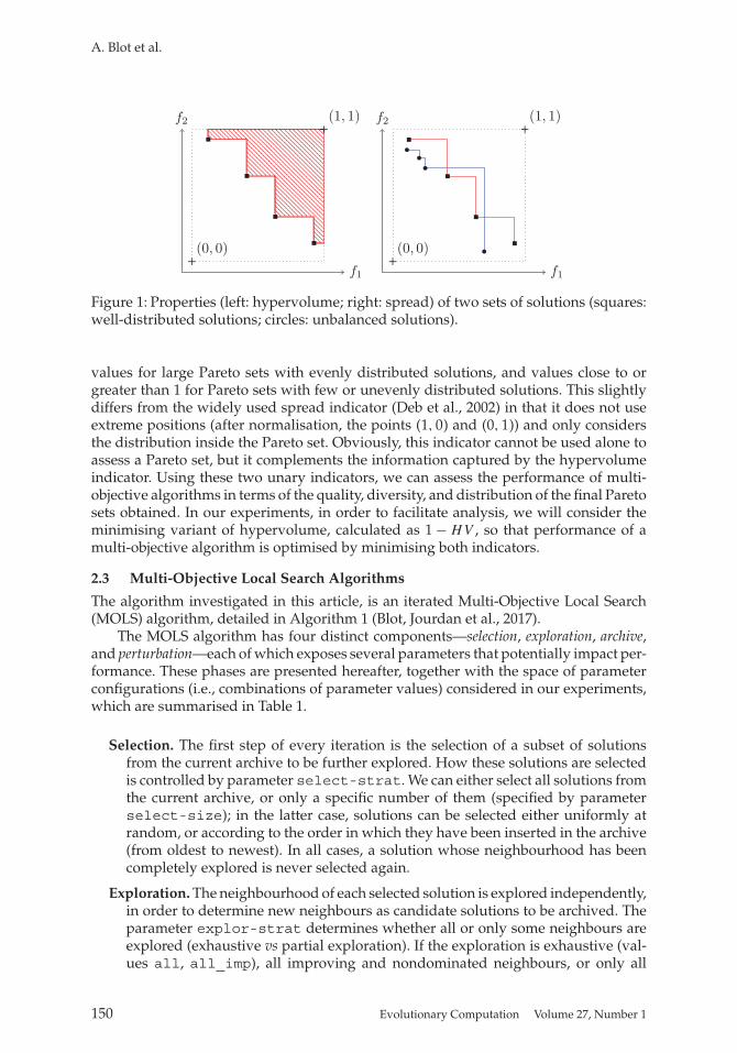
Hypervolume (HV) is by far the most broadly used performance indicator in the lit-erature on multi-objective optimisation (Riquelme et al., 2015). Assuming normalisedobjective values in [0, 1], the unary hypervolume measures the volume between thePareto set of solutions and the point (1, 1) (see Figure 1, left). HV is primarily a con-vergence indicator, but also captures information about the diversity of the front ofsolutions.

As a complementary indicator, we use a variant of spread to capture the distribu-tional properties of the Pareto set. Refer to Figure 1, right, which shows two sets of solu-tions, one well-distributed (squares) and the other unbalanced (circles). Given a Paretoset S, ordered regarding the first criterion, we define

�′ :=∑|S|−1

i=1 |di − d̄|(|S| − 1) · d̄

,

where d̄ denotes the average over the Euclidean distances di for i ∈ [1, |S| − 1] betweenadjacent solutions on the ordered set S. This indicator is to be minimised; it takes small

Evolutionary Computation Volume 27, Number 1 149

A. Blot et al.

Figure 1: Properties (left: hypervolume; right: spread) of two sets of solutions (squares:well-distributed solutions; circles: unbalanced solutions).

values for large Pareto sets with evenly distributed solutions, and values close to orgreater than 1 for Pareto sets with few or unevenly distributed solutions. This slightlydiffers from the widely used spread indicator (Deb et al., 2002) in that it does not useextreme positions (after normalisation, the points (1, 0) and (0, 1)) and only considersthe distribution inside the Pareto set. Obviously, this indicator cannot be used alone toassess a Pareto set, but it complements the information captured by the hypervolumeindicator. Using these two unary indicators, we can assess the performance of multi-objective algorithms in terms of the quality, diversity, and distribution of the final Paretosets obtained. In our experiments, in order to facilitate analysis, we will consider theminimising variant of hypervolume, calculated as 1 − HV , so that performance of amulti-objective algorithm is optimised by minimising both indicators.

2.3 Multi-Objective Local Search Algorithms

The algorithm investigated in this article, is an iterated Multi-Objective Local Search(MOLS) algorithm, detailed in Algorithm 1 (Blot, Jourdan et al., 2017).

The MOLS algorithm has four distinct components—selection, exploration, archive,and perturbation—each of which exposes several parameters that potentially impact per-formance. These phases are presented hereafter, together with the space of parameterconfigurations (i.e., combinations of parameter values) considered in our experiments,which are summarised in Table 1.

Selection. The first step of every iteration is the selection of a subset of solutionsfrom the current archive to be further explored. How these solutions are selectedis controlled by parameter select-strat. We can either select all solutions fromthe current archive, or only a specific number of them (specified by parameterselect-size); in the latter case, solutions can be selected either uniformly atrandom, or according to the order in which they have been inserted in the archive(from oldest to newest). In all cases, a solution whose neighbourhood has beencompletely explored is never selected again.

Exploration. The neighbourhood of each selected solution is explored independently,in order to determine new neighbours as candidate solutions to be archived. Theparameter explor-strat determines whether all or only some neighbours areexplored (exhaustive vs partial exploration). If the exploration is exhaustive (val-ues all, all_imp), all improving and nondominated neighbours, or only all



improving neighbours, are added as candidates, respectively. Otherwise, explo-ration is terminated when a given number (parameter explor-size) of eitherimproving (values imp, imp_ndom) or nondominated (value ndom) neighbourshave been found and added as candidates. Nondominated neighbours evaluated


A. Blot et al.

Table 1: MOLS parameter space (10 920 configurations).

Phase Parameter Parameter values

Selection select-strat {all, rand, newest, oldest}Selection select-size {1, 3, 10}Exploration explor-strat {all, all_imp, imp, imp_ndom, ndom}Exploration explor-ref {sol, arch}Exploration explor-size {1, 3, 10}Archive bound-size {20, 50, 100, 1000}Perturbation perturb-strat {kick, kick_all, restart}Perturbation perturb-size {1, 5, 10}Perturbation perturb-strength {3, 5, 10}

Selection: (1 + 3 × 3) combinations; Exploration: (1 + 2 + 3 × 2 × 3); Perturbation: (3 × 3 + 3 + 1); Total: 10 ×21 × 13 × 4 = 10920 configurations.

during an imp_ndom exploration are also added as candidates. The parameterexplor-ref corresponds to the reference of the exploration and specifies if the“improving” and “nondominating” criteria are computed using the current solu-tion (being explored, value sol) or the current set of all selected solution (valuearch).

Archive. When all solutions selected from the archive are explored, the resulting can-didates are added to the archive, and Pareto-dominated solutions are filtered out.If the size of the archive exceeds the value of parameter bound-size, excess solu-tions are selected and removed uniformly at random, in order to limit explorationwithin the same region of the search space.

Perturbation. When the inner termination criterion is met, the neighbourhood ex-ploration is stopped and a perturbation of the current archive is applied, in or-der to diversify the search. The parameter perturb-strat specifies the pertur-bation mechanism. Either new solutions, generated uniformly at random (valuerestart) are considered, or a kick move (values kick, kick_all) is applied toa given number of solutions (parameter perturb-size), or all solutions of thearchive, respectively. A solution selected for a kick move is replaced by a solutionreached by given number (parameter perturb-strength) of search steps, per-formed sequentially and uniformly at random within the given neighbourhood.

3 Automatic Algorithm Configuration for Multi-Objective Problems

The goal of automatic algorithm configuration (AAC) is to automatically determine a con-figuration (i.e., parameter setting) that optimises the performance of a given algorithmfor a given class of problem instances. In this context, we call the algorithm whose pa-rameters are being optimised the target algorithm and the procedure that configures thetarget algorithm a configurator.

Algorithm configuration is a machine learning process, whose general concept isillustrated in Figure 2. It involves making a prediction of the optimal configuration ofthe target algorithm over a training dataset, usually relative to a given running timeor computational budget. The configurations resulting from this training are then re-evaluated on a disjoint test dataset to ensure the unbiasedness of the final prediction.



Figure 2: Automatic configuration of a given parameterised target algorithm for a givenset of problem instances.

Given a parameterised target algorithm A, a space � of configurations of A, a dis-tribution of instances D, a performance indicator o : � × D → R, and a statistical pop-ulation parameter E; the algorithm configuration problem consists in optimising theaggregated performance of the target algorithm A across all instances i ∈ D, as given inEq. 1 (in which Aθ denotes the algorithm obtained by associating the configuration θ tothe target algorithm A). {

optimise E[o(Aθ, i), i ∈ D]

subject to θ ∈ �.(1)

Algorithm configuration supposes that the limit implied by Eq. 1 exists and is finite. Themost commonly used statistical parameter is the simple average of the performance ofthe target algorithm.

AAC has traditionally been defined as a single-objective optimisation problem,with either running time or solution quality as the optimisation objective. Recently (Blotet al., 2016), AAC has been extended to simultaneously deal with multiple performancemetrics of a given target algorithm, giving rise to the notion of multi-objective auto-matic algorithm configuration (MO-AAC). While in single-objective AAC (SO-AAC),the performance of the target algorithm is represented as a scalar value and the output ofthe configurator is a single configuration, in MO-AAC, target algorithm performance isvector-valued, and the configurator produces a Pareto set of optimised configurations.

In our experiments, we will compare two SO-AAC approaches and one MO-AAC approach optimising the performance of a multi-objective local search algorithm.Specifically, as in previous work, we consider three distinct AAC approaches (Blot, Per-net et al., 2017):

HV , a SO-AAC approach that optimises the hypervolume indicator only.

HV+�′, a SO-AAC approach that optimises a weighted sum of hypervolume (witha 0.75 coefficient) and �′ spread (with a 0.25 coefficient).

HV ||�′, a MO-AAC approach that simultaneously considers hypervolume and �′

spread.

The latter two approaches are motivated by the previously mentioned belief thatthe performance assessment of multi-objective algorithms benefits from the use ofmultiple performance indicators (Zitzler et al., 2003). By comparing HV to the twoother configuration approaches, we aim to assess this belief in the context of auto-matic configuration of MOLS algorithms. Furthermore, by comparing HV +�′ andHV ||�′, we intend to assess the benefits of MO-ACC compared to SO-ACC with


A. Blot et al.

aggregated performance metrics. The aggregation coefficients (0.75 and 0.25) have beenset since the �′ indicator is a complementary measure to the hypervolume that enablesto focus on convergence first and diversity second.

While numerous state-of-the-art SO-AAC procedures can be found in the litera-ture, including irace (López-Ibáñez et al., 2016), based on statistical racing, SMAC (Hut-ter et al., 2011), based on regression models, and ParamILS (Hutter et al., 2009), basedon iterated local search, only a few MO-AAC procedures exist, including SPRINT-race(Zhang et al., 2015) and MO-ParamILS (Blot et al., 2016). In the following, we useParamILS, one of the most widely used SO-AAC procedures, and MO-ParamILS, itsrecent multi-objective extension. Both configurators are based on iterated local searchwithin the space of valid target algorithm configurations enabling a fair comparisonbetween AAC approaches.

Indeed, SPRINT-race is a very simple and noniterative multi-objective racing proce-dure. Its public implementation requires to fully evaluate every possible configurationon every possible instance that it is not admissible in our context.

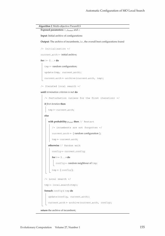
The core algorithm of MO-ParamILS is given by Algorithm 2. Like its predecessorParamILS, it is based on an iterated local search (Lourenço et al., 2003; Hoos and Stützle,2004), in which the incumbents (i.e., the best solutions so far) are iteratively improvedby mean of both local search and perturbation mechanisms. Three parameters are ex-posed: the number r of initial random configurations, a restart probability prestart, andthe number s of random search steps performed in each perturbation phase. The up-date() function performs target algorithms runs and ensures that the different config-urations can be compared, while the archive() function simply discards dominatedconfigurations.

ParamILS and MO-ParamILS start by considering r random configurations, in or-der to compare the initial (usually default) configuration to a few others to makesure of its relevance. Then, they apply a local search procedure, which is based onthe one-exchange neighbourhood, that is, modifying a single parameter value at a time.A tabu mechanism is also used to ensure that the configurator is never stuck. Be-tween iterations, there is a prestart chance to restart the search from a new configuration,uniformly chosen at random from the search space. Otherwise, a perturbation of s ran-dom steps is performed. The main difference between ParamILS and MO-ParamILSis that the former focuses on optimising a single configuration with regard to a sin-gle performance indicator, while the later optimises an archive of configurations, thatis, the set of the current best configurations with regard to the multiple performanceindicators.

Specifically, we used the FocusILS variants of both configurators, since these usu-ally give the best performance. For more details on those configurators, we refer theinterested reader to Hutter et al. (2009) and Blot et al. (2016).

4 Experimental Setup

In this section, we present the two bi-objective permutation problems we used in ourexperiments: the permutation flow-shop scheduling problem (bPFSP) and the travel-ling salesman problem (bTSP). We choose these problems, because they are comple-mentary in the sense that the classical bPFSP naturally involves two strongly correlatedobjectives, while the classical bTSP is constructed in way that gives rise to independentobjectives. We also describe the protocol we use for configuration our multi-objectivelocal search framework for these problems.




A. Blot et al.

4.1 The Bi-Objective Permutation Flow-Shop Scheduling Problem (bPFSP)

The permutation flow-shop scheduling problem (PFSP) involves scheduling a set ofN jobs {J1, . . . , JN } on a set of M machines {M1, . . . ,MM}. Each job Ji is processed se-quentially on each of the M machines, with fixed processing times {pi,1, . . . , pi,M}, andmachines can only process one job at a time. The sequencing of jobs is identical on everymachine, so that a solution may be represented by a permutation of size N . The comple-tion times Ci,j for each job on each machine for a given permutation π = (π1, . . . , πn)are computed using Eq. 2 to Eq. 5.

Cπ1,1 := pπ1,1 (2)

Cπ1,j := Cπ1,j−1 + pπ1,j ∀j ∈ {2, . . . , m} (3)

Cπi,1 := Cπi−1,1 + pπi,1 ∀i ∈ {2, . . . , n} (4)

Cπi,j := max(Cπi−1,j , Cπi ,j−1) + pπi,1 ∀i ∈ {2, . . . , n} ∀j ∈ {2, . . . , m}. (5)The completion time Ck of a job Jk corresponds to its completion time on the last ma-chine Ck,m. In the following, we consider the bi-objective PFSP (bPFSP), minimisingtwo widely studied objectives, makespan Cmax (Eq. 6) and flowtime FT (Eq. 7), wheremakespan is the total completion time of the schedule, and flowtime is the sum of theindividual completion times Ci of the N jobs.

Cmax := maxi∈{1,...,N}

Ci (6)

FT :=N∑

i=1

Ci. (7)

Naturally, these two objectives are strongly coupled via the completion times for theindividual jobs.

Arguably the most widely studied PFSP are those introduced by Taillard (1993),with numbers of jobs, N ∈ {20, 50, 100, 200, 500} and numbers of machines, M ∈{5, 10, 20}. There are 10 instances for every valid (N,M ) combination in Taillard’s bench-mark set.

In the following, we consider three types of PFSP instance sets, characterised bytheir number of jobs, N ∈ {50, 100, 200} and a fixed number of machines set to M = 20.The higher the number of jobs, the more challenging the instances tend to be. For theexhaustive analysis and the test phase of the three AAC approaches, we use the 10 Tail-lard instances for each of those N values. For the training phase of the AAC approaches,we used a different, completely disjoint, set of instances, composed by newly generatedTaillard-like instances. We generated 30 of these instances for each M ∈ {50, 100, 200},using the original generation procedure.

When running MOLS on bPFSP instances, we initialise the search using the 2-phaselocal search algorithm by Dubois-Lacoste et al. (2011), which is based an iterated greedy(IG) procedure (Ruiz and Stützle, 2007). This method is known to produce relativelygood and well-distributed solutions sets. We use 25% of the overall time budget forthis initialisation, and 75% for the remainder of each MOLS run. Classical PFSP neigh-bourhoods include the exchange neighbourhood, where the positions of two jobs areexchanged, and the insertion neighbourhood, where one job is reinserted at another po-sition in the permutation. In this study, we consider a hybrid neighbourhood defined asthe union of the exchange and insertion neighbourhoods, which is known to lead to bet-ter performance than considering each neighbourhood independently (Dubois-Lacosteet al., 2015).



4.2 The Bi-Objective Travelling Salesman Problem (bTSP)

The Travelling Salesman Problem (TSP) can be defined by a complete weighted graphG whose nodes represent cities, while edges corresponds to direct paths between cities.In the symmetric TSP, the graph is undirected, and edge weights correspond to dis-tances between cities. Given a TSP instance G, the goal is to determine a round trip (ortour) passing through every city exactly once such that the overall distance travelled isminimised, that is, a minimum-weight Hamiltonian cycle in G. We note that any Hamil-tonian cycle in G corresponds to a permutation of the cities. The TSP is one of the mostwidely studied combinatorial optimisation problems.

In the following, we consider the bi-objective symmetric TSP (bTSP), in which eachinstance is defined by a graph G as in the standard TSP, but each edge between twonodes i and j have two weights, c1

i,j and c2i,j . We now define the two objectives as the

total distance covered by a given round trip according to each of the two distance ma-trices (d1)i,j and (d2)i,j . Both objectives have to be minimised.

A benchmark set of Euclidean instances (available online1) has been widely used inthe literature to assess the performance of bTSP algorithms (Paquete et al., 2004; Lustand Teghem, 2010; Dubois-Lacoste et al., 2015). These instances were constructed bycombining two independently generated distance matrices, computed using Euclideandistance between cities randomly placed on a two-dimension grid; therefore, unlike inthe case of the bPFSP discussed earlier, the two optimisation objectives are uncorre-lated. The bTSP benchmark set contains six instances each for 100, 300, and 500 cities,meaning 15 different pairwise independent combinations of two instances per bench-mark size. For our exhaustive analysis and the test phase of the three AAC approaches,we used these 15 instances. For the training phase of the AAC approaches, we used adifferent, completely disjoint, set of newly generated instances containing 30 instancesfor each number of cities, obtained using the original generator from the DIMACSchallenge.

Each run of MOLS is initialised using the well-known nearest neighbour heuristicapplied to only one of the two objectives, resulting in two greedily constructed tours.Subsequently, we perform local search steps in the classical two-opt neighbourhood, ac-cording to which the neighbours of a given tour are obtained by removing two non-adjacent edges and reconnecting the resulting fragments by two new edges such that adifferent tour is obtained (Croes, 1958).

4.3 AAC Protocol

Our MO-ParamILS multi-objective algorithm configuration protocol proceeds in threephases: training, validation, and test.

Training: In the training phase, MO-ParamILS is independently run multiple timeson a given training set of instances; each of these runs produces a Pareto set ofconfigurations. Multiple runs of MO-ParamILS are used, because individual runscan suffer from stagnation and to make effective use of parallel computing re-sources. However, as different MO-ParamILS runs usually use different subsetsof the given training set, the configurations obtained from them cannot be fairlycompared to each other.

1https://eden.dei.uc.pt/∼paquete/tsp


A. Blot et al.

Table 2: Small version of the MOLS parameter space (300 configurations).

Phase Parameter Parameter values

Selection select-strat {all, rand, oldest}Selection select-size {1, 10}Exploration explor-strat {imp, imp_ndom, ndom}Exploration explor-ref {sol, arch}Exploration explor-size {1, 10}Archive bound-size {1000}Perturbation perturb-strat {kick, kick_all, restart}Perturbation perturb-size {10}Perturbation perturb-strength {3, 10}

Selection: (1 + 2 × 2) combinations; Exploration: (3 × 2 × 2); Perturbation: (2 × 2 + 1); Total: 5 × 12 × 5 = 300configurations.

Validation: To fairly compare configurations obtained from different MO-ParamILSruns and to reduce the number of configurations ultimately evaluated in the testphase, every configuration from the training phase is evaluated on the same, fixedsubset of training instances. Based on the performance measurements thus ob-tained, Pareto-dominated configurations are removed.

Test: The Pareto set of configurations obtained from the validation phase is evaluatedagain, on a set of test instances that does not contain any of the instances used fortraining or validation. Again, Pareto-dominated configurations are removed.

Using this protocol, we compare the three AAC approaches described in Section 3.In the case of the HV approach, ParamILS is used during the training phase to onlyoptimise the hypervolume of the target algorithm, since the configuration scenario issingle-objective. However, during the subsequent validation and test phases, the con-figurations resulting from the single-objective training are assessed using both hyper-volume and �′ spread separately, in a Pareto way. Ultimately, it is expected that thisapproach only finds good hypervolume values and disregards the �′ spread value.Similarly, the HV +�′ approach uses ParamILS during the training phase to optimisean aggregation of hypervolume and �′ spread, while the assessment of the validationand test phases are then performed in a Pareto way.

These two SO-AAC approaches constitute the baseline against which our MO-AACapproach is compared to. While they focus on specific directions of the multi-objectivespace and use an optimisation criterion less complete than the final evaluation, they rep-resent the performance that our multi-objective approach will have to at least match. Wenote that this makes effective use of an off-the-shelf SO-AAC procedure, while takinginto account the multi-objective nature of the algorithm configuration problem we areultimately trying to solve.

In the following, this protocol is used in conjunction with two different configu-rations spaces (in the training phase). First, we consider a small configuration space of300 configurations, described in Table 2. This smaller configuration space has been de-fined based on preliminary experiments, in which we informally identified parametersand parameter values most likely to result in good performance of our target algorithmframework. The small size of this search space permits us to perform validation andtesting in an exhaustive way, where the performance of each of the 300 configurations



Table 3: AAC experimental protocol.

Phase Small configuration space Large configuration space

Training No default configuration No default configuration1 random configuration 10 random configurations10 ParamILS runs 20 ParamILS runs100 MOLS runs budget 1000 MOLS runs budgetmax 10 MOLS run per config. max 100 MOLS run per config.

Validation 1 run per instance 1 run per instanceTest 10 runs per instance 10 runs per instance

is assessed on the entire training and test instance sets, respectively. This exhaus-tive analysis of the configuration space enables the comparison of the configurationsresulting from the training phase to ones that may otherwise be never considered.As stated previously, our goal with this analysis is to demonstrate that our AAC ap-proaches can effectively configure a multi-objective local search for solving bi-objectivepermutation problems.

The second configuration space, detailed in Table 1 and already presented in Sec-tion 2, enables the comparison between our three AAC approaches in a much richerspace with 10,920 configurations. We note that, because of the relatively high runningtimes for each configuration and the stochastic nature of our target algorithm, search-ing this space exhaustively would require a computational budget orders of magnitudebeyond that used for the experiments described in the following.

Table 3 summarises the details of our AAC protocol for both configuration spaces.The main differences concern the training phase. For the small (large) configurationspace, ParamILS starts by evaluating a single (10) random configuration, and can exe-cute 100 (1000) MOLS runs before stopping, where each selected configuration cannotbe run more than 10 (100) times. Due to the reduced size of the small configurationspace, only 10 independent runs of ParamILS are performed, compared to 20 runs forthe large space. In the validation phase, the configurations resulting from the trainingphase are evaluated on all training instances, running every configuration once on eachinstance. In the test phase, each of the configurations in the Pareto set obtained fromthe validation phase is run 10 times on every test instance. For both validation and testphases, the performance of each configuration is assessed based on the average hyper-volume and spread values over the runs. Obviously, for the small configuration space,our exhaustive analysis ensures that the performance of all configurations are knownfor all training and test instances, and we will directly use these results in the validationand test phases to avoid recomputing the performance of configurations selected in thetraining phase.

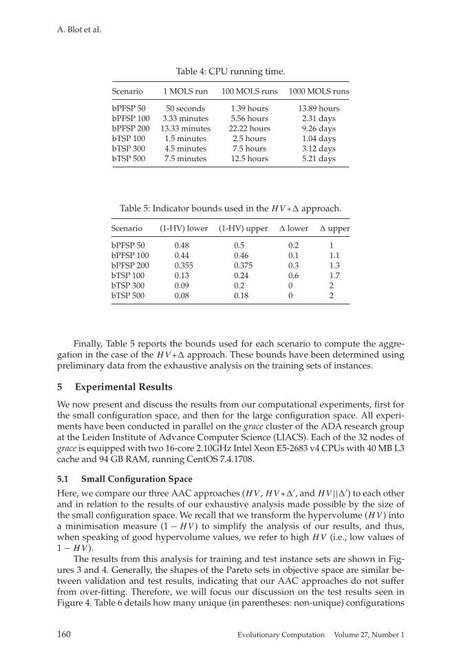
Table 4 details the CPU running time for a single run, 100 runs, and 1000 runs ofa MOLS algorithm. The last two columns correspond to the running time of a singlerun of (MO-)ParamILS on the small and large configuration spaces, without taking intoaccount the slight system time overhead induced by launching the MOLS executable.Note that to obtain the total training time, these durations should be multiplied by thenumber of (MO-)ParamILS runs (10 and 20, respectively). Moreover, the time requiredfor the validation and test steps is not pointed out since it depends on the number ofconfigurations returned by the training step.


A. Blot et al.

Table 4: CPU running time.

Scenario 1 MOLS run 100 MOLS runs 1000 MOLS runs

bPFSP 50 50 seconds 1.39 hours 13.89 hoursbPFSP 100 3.33 minutes 5.56 hours 2.31 daysbPFSP 200 13.33 minutes 22.22 hours 9.26 daysbTSP 100 1.5 minutes 2.5 hours 1.04 daysbTSP 300 4.5 minutes 7.5 hours 3.12 daysbTSP 500 7.5 minutes 12.5 hours 5.21 days

Table 5: Indicator bounds used in the HV+� approach.

Scenario (1-HV) lower (1-HV) upper � lower � upper

bPFSP 50 0.48 0.5 0.2 1bPFSP 100 0.44 0.46 0.1 1.1bPFSP 200 0.355 0.375 0.3 1.3bTSP 100 0.13 0.24 0.6 1.7bTSP 300 0.09 0.2 0 2bTSP 500 0.08 0.18 0 2

Finally, Table 5 reports the bounds used for each scenario to compute the aggre-gation in the case of the HV+� approach. These bounds have been determined usingpreliminary data from the exhaustive analysis on the training sets of instances.

5 Experimental Results

We now present and discuss the results from our computational experiments, first forthe small configuration space, and then for the large configuration space. All experi-ments have been conducted in parallel on the grace cluster of the ADA research groupat the Leiden Institute of Advance Computer Science (LIACS). Each of the 32 nodes ofgrace is equipped with two 16-core 2.10GHz Intel Xeon E5-2683 v4 CPUs with 40 MB L3cache and 94 GB RAM, running CentOS 7.4.1708.

5.1 Small Configuration Space

Here, we compare our three AAC approaches (HV , HV +�′, and HV ||�′) to each otherand in relation to the results of our exhaustive analysis made possible by the size ofthe small configuration space. We recall that we transform the hypervolume (HV ) intoa minimisation measure (1 − HV ) to simplify the analysis of our results, and thus,when speaking of good hypervolume values, we refer to high HV (i.e., low values of1 − HV ).

The results from this analysis for training and test instance sets are shown in Fig-ures 3 and 4. Generally, the shapes of the Pareto sets in objective space are similar be-tween validation and test results, indicating that our AAC approaches do not sufferfrom over-fitting. Therefore, we will focus our discussion on the test results seen inFigure 4. Table 6 details how many unique (in parentheses: non-unique) configurations



Figure 3: Exhaustive analysis on training instances (left: bPFSP; right: bTSP). ×: HV

approach, o: HV+�′ approach, �: HV ||�′ approach, +: exhaustive analysis.


A. Blot et al.

Figure 4: Exhaustive analysis on test instances (left: bPFSP; right: bTSP). ×: HV ap-proach, o: HV +�′ approach, �: HV ||�′ approach, +: exhaustive analysis.



Table 6: Number of configurations after training, validation, and testing.

Small space Large space

Scenario Approach Configs Pareto Final Configs Pareto Final

bPFSP 50 HV 10 2 2 20 2 2HV+�′ 10 4 2 10 2 2HV ||�′ 32 (38) 9 7 145 14 11

bPFSP 100 HV 10 4 3 19 (20) 1 1HV +�′ 8 (10) 3 3 20 4 2HV ||�′ 36 (42) 12 6 171 (172) 27 19

bPFSP 200 HV 10 3 3 20 4 3HV +�′ 9 (10) 5 3 16 (20) 2 2HV ||�′ 29 (39) 11 8 111 (117) 14 9

bTSP 100 HV 6 (10) 1 1 15 (20) 2 1HV+�′ 6 (10) 2 2 15 (20) 6 4HV ||�′ 16 (26) 3 3 62 (73) 11 5

bTSP 300 HV 9 (10) 2 2 13 (20) 4 2HV+�′ 9 (10) 5 5 12 (20) 5 2HV ||�′ 33 (41) 8 6 107 (130) 18 12

bTSP 500 HV 6 (10) 5 4 16 (20) 4 4HV+�′ 8 (10) 5 4 14 (20) 3 2HV ||�′ 36 (40) 12 11 135 (145) 25 22

were found by each AAC approach, and how many of these survived the validation andtest phases. (Recall that Pareto-dominated configurations are pruned in those phases.)Figure 5 shows the parameter distribution of the 300 configurations on test instancesaccording to our three selection mechanisms (crosses: + × �, polygons: ��, and cir-cles: o⊕⊗) and our three exploration strategies (red: +�o, green: ×�⊕, and blue: � ⊗).Finally, Tables 7 to 12 list the Pareto-optimal configurations within the small configura-tion space. A “∗” symbol indicates that the value of the respective parameter does notimpact the performance of the configured MOLS when the other parameter values areheld fixed at the values shown. Conversely, when a specific parameter is shown, anydeviation from it will reduce performance.

First, we will discuss the results for the bPFSP. None among the 300 possible config-urations simultaneously achieves good hypervolume and spread values (see Figure 4);the Pareto front is distinctly non-convex. While for the smallest scenario with 50 jobs,most of all configurations achieve good hypervolume values (i.e., low 1 − HV ), suchconfigurations get rarer as the number of jobs increases. This result was expected, sinceit is known that larger bPFSP instance are harder for multi-objective local search. Exam-ining these results in more detail, we observe that the imp exploration strategy alwaysobtains rather bad hypervolume values (see Figure 5). For 50 jobs, this strategy leadsto better spread values; however, this tends to be no longer true for larger instances.For the three instance sizes, the imp-ndom and ndom strategies appear to give betterperformance in terms of hypervolume.

All three approaches find very good, even near-optimal configurations—in partic-ular, HV ||�′, which achieves spreads over the entire Pareto-front. The 10 configuratorruns of HV and HV +�′ produce close to 10 unique configurations each (see Table 6),


A. Blot et al.

Figure 5: Exhaustive analysis parameter distribution on test instances (left: bPFSP; right:bTSP); Selection strategy: +×�: all (crosses), ��: oldest (polygons), o⊕⊗: rand(circles); Exploration strategy: +�o: imp (red), ×�⊕: imp_ndom (green), � ⊗: ndom(blue).



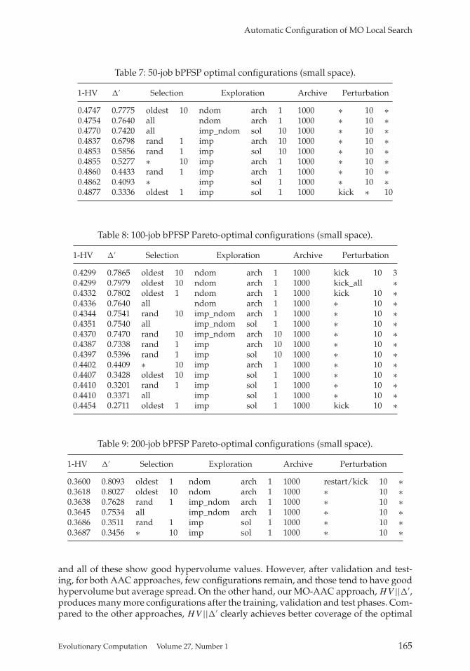
Table 7: 50-job bPFSP optimal configurations (small space).

1-HV �′ Selection Exploration Archive Perturbation

0.4747 0.7775 oldest 10 ndom arch 1 1000 ∗ 10 ∗0.4754 0.7640 all ndom arch 1 1000 ∗ 10 ∗0.4770 0.7420 all imp_ndom sol 10 1000 ∗ 10 ∗0.4837 0.6798 rand 1 imp arch 10 1000 ∗ 10 ∗0.4853 0.5856 rand 1 imp sol 10 1000 ∗ 10 ∗0.4855 0.5277 ∗ 10 imp arch 1 1000 ∗ 10 ∗0.4860 0.4433 rand 1 imp arch 1 1000 ∗ 10 ∗0.4862 0.4093 ∗ imp sol 1 1000 ∗ 10 ∗0.4877 0.3336 oldest 1 imp sol 1 1000 kick ∗ 10

Table 8: 100-job bPFSP Pareto-optimal configurations (small space).


0.4299 0.7865 oldest 10 ndom arch 1 1000 kick 10 30.4299 0.7979 oldest 10 ndom arch 1 1000 kick_all ∗0.4332 0.7802 oldest 1 ndom arch 1 1000 kick 10 ∗0.4336 0.7640 all ndom arch 1 1000 ∗ 10 ∗0.4344 0.7541 rand 10 imp_ndom arch 1 1000 ∗ 10 ∗0.4351 0.7540 all imp_ndom sol 1 1000 ∗ 10 ∗0.4370 0.7470 rand 10 imp_ndom arch 10 1000 ∗ 10 ∗0.4387 0.7338 rand 1 imp arch 10 1000 ∗ 10 ∗0.4397 0.5396 rand 1 imp sol 10 1000 ∗ 10 ∗0.4402 0.4409 ∗ 10 imp arch 1 1000 ∗ 10 ∗0.4407 0.3428 oldest 10 imp sol 1 1000 ∗ 10 ∗0.4410 0.3201 rand 1 imp sol 1 1000 ∗ 10 ∗0.4410 0.3371 all imp sol 1 1000 ∗ 10 ∗0.4454 0.2711 oldest 1 imp sol 1 1000 kick 10 ∗

Table 9: 200-job bPFSP Pareto-optimal configurations (small space).


0.3600 0.8093 oldest 1 ndom arch 1 1000 restart/kick 10 ∗0.3618 0.8027 oldest 10 ndom arch 1 1000 ∗ 10 ∗0.3638 0.7628 rand 1 imp_ndom arch 1 1000 ∗ 10 ∗0.3645 0.7534 all imp_ndom arch 1 1000 ∗ 10 ∗0.3686 0.3511 rand 1 imp sol 1 1000 ∗ 10 ∗0.3687 0.3456 ∗ 10 imp sol 1 1000 ∗ 10 ∗

and all of these show good hypervolume values. However, after validation and test-ing, for both AAC approaches, few configurations remain, and those tend to have goodhypervolume but average spread. On the other hand, our MO-AAC approach, HV ||�′,produces many more configurations after the training, validation and test phases. Com-pared to the other approaches, HV ||�′ clearly achieves better coverage of the optimal


A. Blot et al.

Table 10: 100-city bTSP Pareto-optimal configurations (small space).


0.1372 0.7389 rand 10 imp_ndom sol 10 1000 ∗ 10 ∗0.1431 0.6572 all imp_ndom sol 10 1000 restart0.1443 0.6544 all imp_ndom arch 10 1000 restart0.1902 0.6488 oldest 1 ndom sol 1 1000 kick 10 3



0.1003 1.3582 oldest 10 imp_ndom sol 1 1000 ∗ 10 ∗0.1006 1.3417 oldest 10 imp_ndom sol 10 1000 ∗ 10 ∗0.1092 1.0409 oldest 10 ndom sol 10 1000 ∗ 10 ∗0.1128 0.7933 rand 10 imp_ndom arch 1 1000 ∗ 10 ∗0.1129 0.7880 rand 1 imp_ndom arch 1 1000 ∗ 10 ∗0.1171 0.5003 rand 1 imp sol 10 1000 restart0.1183 0.2288 rand 1 imp sol 1 1000 restart0.1190 0.0409 rand 1 imp arch 1 1000 restart



0.0841 1.3767 oldest 10 imp_ndom sol 1 1000 ∗ 10 ∗0.0989 1.2983 oldest 1 imp_ndom arch 10 1000 ∗ 10 ∗0.1003 1.2897 oldest 10 ndom arch 10 1000 ∗ 10 ∗0.1015 1.1290 oldest 10 ndom sol 10 1000 ∗ 10 ∗0.1159 1.0080 rand ∗ imp_ndom arch 1 1000 ∗ 10 ∗0.1403 0.8468 oldest 10 ndom arch 1 1000 kick 10 ∗0.1616 0.4420 rand 1 imp sol 10 1000 ∗ 10 ∗0.1624 0.0000 rand 1 imp ∗ 1 1000 ∗ 10 ∗

Pareto set of configurations (Figure 4). Note that all three approaches use the same timebudget for configuration, the number of final solutions being strongly dependant of thekind (single-objective or multi-objective) of AAC used for training.

Regarding the nature of the configurations, we observe a trend across the three in-stance sizes (Tables 7 to 9): The best hypervolume is always reached with the oldestselection strategy, the ndom exploration strategy, and the arch exploration reference setchoice. Slightly worse hypervolume, but better spread is achieved using the imp_ndomexploration strategy. Finally, the best spread values are obtained from configurationsusing the imp exploration strategy, although this comes at the cost of rather bad hyper-volume. In almost every case, the perturbation strategy did not significantly impact theperformance of the nondominated configurations.



Our results on the bTSP differ markedly from those on the bPFSP. Firstly, we observethat the shape of the Pareto-optimal front of configurations varies with instance size:While it is convex for 100 cities with some degree of correlation between hypervolumeand spread, for larger instances, the correlation between the two performance indicatorsdecreases, and the front becomes non-convex. In contrast to the bPFSP, where the twoobjectives were correlated, for our bTSP benchmark sets, the objectives are completelyindependent; therefore, the final archives are much bigger, as there exists a richer spaceof trade-off solutions. The impact on spread is evident from Figure 4; values above 1correspond to two tightly clustered sets of solutions separated by a large gap that therespective configuration of MOLS failed to cover, and spread values of 0 correspond tofinal sets containing only two solutions, which are produced when the imp explorationstrategy fails to sufficiently diversify.

Our HV configuration approach produced few configurations, achieving near-optimal hypervolume. HV +�′ produced weak training results on the 100-city instances,but worked well on the 300-city instances, because of the shape of the Pareto-optimalfront. As for the bPFSP, HV ||�′ found many more configurations and achieved far bettercoverage of the Pareto front. In our test instances from the literature, all three AAC ap-proaches produced optimal configurations for 100-city instances, HV +�′ and HV ||�′

still did on 300-city instances, and only HV ||�′ managed to find most of the optimalconfigurations on the 500-city instance (see Figure 4).

Analysing the MOLS configurations in more detail, those that achieve the best hy-pervolume values always use the imp_ndom exploration strategy with the sol refer-ence set. While for 300- and 500-city instances, the oldest selection strategy is pre-ferred, for 100 cities, the more common rand selection strategy performs better. Simi-larly to the bPFSP, the choice of perturbation mechanism does not significantly impactthe performance of optimal configurations.

For both problems, within the small configuration space, all three AAC approachesare able to find configurations very close to the true Pareto-front. The two SO-AACapproaches strongly favour the hypervolume indicator, while the MO-AAC approachis able to accurately cover the full range of Pareto-optimal configurations.

5.2 Large Configuration Space

In this section, our three AAC approaches are now tested against a much larger searchspace, in order to study their scalability.

Figure 6 shows the final configurations produced by all three AAC approaches forour six benchmarks (two problems, three instance sizes). We also show the configura-tions of the smaller set of configurations that we exhaustively evaluated in Section 5.1,in order to show that these final configurations map very closely those found within thesmall space, which suggests that the small space indeed captures the high-performanceconfigurations from the much larger space and, more importantly, demonstrates thatour AAC approaches effectively finds such configurations. In the following, we willfocus on the performance of our three AAC approaches.

Both SO-AAC approaches, HV and HV +�′, produced few nondominated configu-rations in their final testing phase—typically between 2 and 4 on each instance set (seeTable 6). As one might expect, HV always finds a final configuration with near-optimalhypervolume. The results for HV+�′ are similar to those for HV for the bPFSP, butmarkedly different on our bTSP benchmarks. For 100-city bTSP instances, HV +�′ cov-ers the Pareto front, while for 300 cities, it finds the two extreme configurations, dueto accidentally well-adapted weights used for aggregating hypervolume and spread.


A. Blot et al.

Figure 6: Large-scale analysis on test instances (left: bPFSP; right: bTSP). x: HV ap-proach, o: HV +�′ approach, �: HV ||�′ approach, +: exhaustive analysis.



However, due to the non-convex shape of the front, no trade-off configurations arefound between these extremes. For 500-city instances, HV +�′ only finds configurationswith near-optimal hypervolume, similar to what we observed for the bPFSP.

On the other hand, our MO-AAC approach, HV ||�′, consistently provides manymore nondominated configurations, except for the small 100-city bTSP instance set,where the Pareto front is completely covered by all three approaches. In all cases, thesets of configurations found by HV ||�′ are very well distributed over the entire front ofoptimal configurations. Although HV +�′ sometimes finds better configurations (e.g.,on the 100- and 200-jobs bPFSP scenarios), HV ||�′ always produces configurations withsimilar performance.

Overall, our MO-AAC approach, HV ||�′, produces substantially better results thanthe two SO-AAC approaches, HV and HV +�′. HV finds excellent sets of configura-tions with respect to hypervolume, but provides only very few of those and conse-quently fails to achieve good spread. HV+�′ sometimes provides better results and,under favourable circumstances, can cover the entire set of Pareto-optimal configura-tions; however, especially for more challenging scenarios, its performance is similar tothat of HV . The main drawback of this approach is the requirement of a costly prelim-inary step for calibrating the weights used for aggregating the two optimisation objec-tives. Finally, HV ||�′, our native MO-AAC approach, always efficiently covers the entirePareto-front of configurations, while still finding sets of configurations with excellenthypervolume, as produced by the two SO-AAC approaches.

6 Conclusion

In this article, we have studied the question how to best approach the automated con-figuration of multi-objective optimisation algorithms. From the literature, it is knownthat no single metric completely characterises the performance of MOO algorithms,and that therefore, it is best to evaluate such algorithms using multiple complementaryperformance metrics. Consistent with this insight, we have studied the use of multi-objective configuration techniques for MOO algorithms, contrasting two approachesbuilt around a standard, single-objective configuration procedure with one using anatively multi-objective algorithm configurator. Substantially expanding on our own,preliminary work in this area, we have conducted extensive experiments with a highly-parametric local search framework, MOLS, applied to two well-known MOO prob-lems, the bi-objective permutation flowshop and travelling salesman problems. Wehave found strong evidence that automated configuration of highly parametric MOOframeworks such as ours is effectively possible using existing techniques and, moreimportantly, that indeed, by using a natively multi-objective algorithm configurator—here, MO-ParamILS (Blot et al., 2016)—the best configuration results can be achieved.Specifically, using MO-ParamILS, we could consistently obtain large and diverse setsof configurations of our MOLS framework.

In future work, we intend to study how the degree of correlation between the ob-jectives of a given MOO problem impacts the performance of our automated algorithmconfiguration approaches and that of the configurations thus obtained. Our results pre-sented here already provide some evidence for qualitative differences arising from veryhigh and very low degrees of correlation, as found in the bi-objective PFSP and TSP, re-spectively, but it is yet to be determined to which degree these findings are independentof other differences between these benchmark problems.

We also believe that it would be very interesting to expand the investigation pre-sented here to other types of MOO problems—notably, to problems from machine


A. Blot et al.

learning and data mining, whose design and calibration usually gives rise to trade-offsbetween several performance objectives, such as sensitivity and specificity, thus provid-ing a new direction for the area of automated machine learning (AutoML).

References

Blot, A., Hoos, H. H., Jourdan, L., Marmion, M.-É., and Trautmann, H. (2016). MO-ParamILS: Amulti-objective automatic algorithm configuration framework. In Proceedings of the Learningand Intelligent Optimization 10 Conference, pp. 32–47.

Blot, A., Jourdan, L., and Kessaci-Marmion, M.-É. (2017). Automatic design of multi-objectivelocal search algorithms: Case study on a bi-objective permutation flowshop schedulingproblem. In Proceedings of the Genetic and Evolutionary Computation 2017 Conference, pp. 227–234.

Blot, A., Pernet, A., Jourdan, L., Kessaci-Marmion, M.-É., and Hoos, H. H. (2017). Automaticallyconfiguring multi-objective local search using multi-objective optimisation. In Proceedings ofthe Evolutionary Multi-Criterion Optimization 2017 Conference, pp. 61–76.

Croes, G. A. (1958). Amethod for solving traveling-salesman problems. Operations Research, 6:791–812.

Deb, K., Pratap, A., Agarwal, S., and Meyarivan, T. (2002). A fast and elitist multiobjective geneticalgorithm: NSGA-II. IEEE Transactions on Evolutionary Computation, 6(2):182–197.

Dubois-Lacoste, J., López-Ibáñez, M., and Stützle, T. (2011). A hybrid TP+PLS algorithm for bi-objective flow-shop scheduling problems. Computers & Operations Research, 38(8):1219–1236.

Dubois-Lacoste, J., López-Ibáñez, M., and Stützle, T. (2015). Anytime Pareto local search. EuropeanJournal of Operational Research, 243(2):369–385.

Hoos, H. H., and Stützle, T. (2004). Stochastic local search: Foundations & applications. San Francisco:Elsevier/Morgan Kaufmann.

Hutter, F., Hoos, H. H., and Leyton-Brown, K. (2011). Sequential model-based optimization forgeneral algorithm configuration. In Proceedings of the Learning and Intelligent Optimization 5Conference, pp. 507–523.

Hutter, F., Hoos, H. H., Leyton-Brown, K., and Stützle, T. (2009). ParamILS: An automatic algo-rithm configuration framework. Journal of Artificial Intelligence Research, 36:267–306.

Hutter, F., Hoos, H. H., and Stützle, T. (2007). Automatic algorithm configuration based on localsearch. In Proceedings of the Twenty-Second AAAI Conference on Artificial Intelligence, pp. 1152–1157.

Knowles, J., and Corne, D. (2002). On metrics for comparing nondominated sets. In IEEE Congresson Evolutionary Computation, Vol. 1, pp. 711–716.

López-Ibáñez, M., Dubois-Lacoste, J., Cáceres, L. P., Birattari, M., and Stützle, T. (2016). The iracepackage: Iterated racing for automatic algorithm configuration. Operations Research Perspec-tives, 3:43–58.

López-Ibáñez, M., and Stützle, T. (2012). The automatic design of multi-objective ant colony op-timization algorithms. IEEE Transactions on Evolutionary Computation, 16(6):861–875.

Lourenço, H., Martin, O., and Stützle, T. (2003). Iterated local search. In Handbook of metaheuristics,pp. 320–353. Berlin: Springer.

Lust, T., and Teghem, J. (2010). Two-phase Pareto local search for the biobjective traveling sales-man problem. Journal of Heuristics, 16(3):475–510.



Murata, T., and Ishibuchi, H. (1998). A multi-objectives genetic local search algorithm and itsapplication flow-shop scheduling. IEEE Transaction System, 28(3):392–403.

Okabe, T., Jin, Y., and Sendhoff, B. (2003). A critical survey of performance indices for multi-objective optimisation. In IEEE Congress on Evolutionary Computation, Vol. 2, pp. 878–885.

Paquete, L., Chiarandini, M., and Stützle, T. (2004). Pareto local optimum sets in the biobjectivetraveling salesman problem: An experimental study. In Metaheuristics for multiobjective opti-misation, pp. 177–199. New York: Springer.

Riquelme, N., von Lücken, C., and Barán, B. (2015). Performance metrics in multi-objective opti-mization. In Proceedings of the 2015 Latin American Computing Conference, pp. 1–11.

Ruiz, R., and Stützle, T. (2007). A simple and effective iterated greedy algorithm for the permu-tation flowshop scheduling problem. European Journal of Operational Research, 177(3):2033–2049.

Taillard, E. (1993). Benchmarks for basic scheduling problems. European Journal of Operational Re-search, 64(2):278–285.

Zhang, T., Georgiopoulos, M., and Anagnostopoulos, G. C. (2015). SPRINT multi-objective modelracing. In Proceedings of the 2015 Genetic and Evolutionary Computation Conference, pp. 1383–1390.

Zitzler, E., and Thiele, L. (1999). Multiobjective evolutionary algorithms: A comparative casestudy and the strength Pareto approach. IEEE Transactions on Evolutionary Computation,3(4):257–271.

Zitzler, E., Thiele, L., Laumanns, M., Fonseca, C. M., and da Fonseca, V. G. (2003). Performanceassessment of multiobjective optimizers: An analysis and review. IEEE Transactions on Evo-lutionary Computation, 7(2):117–132.


Documents

AutomaticConfigurationofMulti-Objective