Embed Size (px)
Citation preview
FACULDADE DE BIOCIÊNCIAS
PROGRAMA DE PÓS-GRADUAÇÃO EM ZOOLOGIA
DEMOGRAFIA HISTÓRICA E CONTEMPORÂNEA DE GUEPARDOS (Acinonyx
jubatus) NA NAMÍBIA, ÁFRICA AUSTRAL
Ezequiel Chimbioputo Fabiano
TESE DE DOUTORADO
PONTIFÍCIA UNIVERSIDADE CATÓLICA DO RIO GRANDE DO SUL
Av. Ipiranga 6681 – Caixa Postal 1429
Fone: (051) 320-3500 – Fax: (051) 339-1564
CEP 90619-900 Porto Alegre – RS
Brasil
2013
PONTIFÍCIA UNIVERSIDADE CATÓLICA DO RIO GRANDE DO SUL
FACULDADE DE BIOCIÊNCIAS
PROGRAMA DE PÓS-GRADUAÇÃO EM ZOOLOGIA
DEMOGRAFIA HISTÓRICA E CONTEMPORÂNEA DE GUEPARDOS (Acinonyx
jubatus) NA NAMÍBIA, ÁFRICA AUSTRAL
Ezequiel Chimbioputo Fabiano
Orientador: Dr. Eduardo Eizirik
TESE DE DOUTORADO
PORTO ALEGRE – RS – BRASIL

2013
i
Sumário
Dedicatória........................................................................................... ii
Acknowledgments................................................................................ iii
Resumo................................................................................................ v
Abstract…………………………………………………………………….. vii
Capitulo I: Introdução Geral……………................................................1-25
Capitulo: II: Inferindo a história demográfica de guepardos da Namibia com
base na análise Bayesiana de dados de microssatélites …………...... 26-77
Capitulo III: Estimativas do tamanho efetivo da população de guepardos
(Acinonyx jubatus) da Namibia: comparação de abordagens analíticas e
avaliação do impacto da variação de taxas vitais................................ 78-127
Capitulo IV: Levantamento e monitoramento de tendências em abundância e
densidade: um estudo de caso de uma população de guepardos (Acinonyx
jubatus) no centro-norte da Namíbia............ ...................................... 128-189
Capítulo V: Padrões de atividade temporais de uma população de guepardos,
no centro-norte da Namíbia..................................................................190-223
Capitulo VI: Discussão geral, conclusões e recomendações............... 224-241

ii
Dedication
This dissertation is dedicated to Almighty God, for giving the opportunity of gaining
new knowledge and to Dr. Martin Mbewe who introduced me to the world of
conservation earlier in 2000.
iii
Acknowledgments
First, I thank God for seeing me through. For being my anchor, source of strength,
motivation, wisdom, calmness, provider, indeed "The Lord is ever present".
Second, I would like to my supervisor Dr. Eduardo Eizirik for taking me in, for your
guidance, patience and perseverance. I did enjoy being under your tutelage and
learning not only about population and conservation genetics but also about human
relations. I appreciated the flexibility you gave me so that I could explore my ideas. I
would like to thank my committee Drs Sandro Luis Bonatto and Nelson
Ferreira Fontoura for advice throughout this journey.
Third, many thanks to my family Marjolein van Dieren, Debora, Delfina and Ambrosio
Fabiano, for keeping me on your prayers and simple being who you are. Marjolein
you are AWESOME!!! Love you all!
Fourth, my gratitude goes to the Cheetah Conservation Fund in particular Dr. Laurie
Marker for believing in me, and Dr. Bruce Brewer. Dr. Anne Schmidt-Küntzel it has
been joyful to work with you. Thank you for always listening and being critical.
Fifth, many thanks to my daughter, Graciela, the best daughter I could have asked
from God. My friends, who where ever present, believed in me, remained true and
honest when necessary and encouraged me, including but not limited to Marianne
De Jonge "Fabiano you will never change when comes to numbers", Veronika
Brinschwitz "Keeping me smiling", Suzie Kenny "Enjoy playing with R", Patricia
Tricorache "Fabiano you can do it, and Manoel Rodrigues "For being a friend, the
laughs and our conversations regarding our PhD journeys".

iv
I would also like to thank everyone else that in one or another way contributed
towards my journey, members of the Central Baptist Church of Porto Alegre, Prayer
Partners around the globe, colleagues from the Genoma in particular Fernanda
Pedone "for introducing me to world of non-invasive genetics", Ana, Analise, Lucas,
Laura; those who took time to help reviewing the dissertation manuscripts in
particular Katherine Forsythe, Marina and Alexandro, Amanda Fabiano, Frederico
Lemos, Likulela, Carolyn among others....
Lastly but not least, I also thank CAPES, the Cheetah Conservation Fund, the
Rufford Small Grants Foundation and the Wildlife Conservation Network for their
financial support and my parents.
v
Resumo
Contexto: A diversidade genética contemporânea de espécies e populações é resultante da interação entre aspectos ecológicos e biológicos das mesmas em relação aos efeitos de processos históricos naturais, bem como ao efeito atual dos humanos. Essas forças causaram alterações no tamanho efetivo da população de muitos elementos da fauna e flora, afetando não só os seus potenciais evolutivos, mas também suas distribuições geográficas. Conseqüentemente, existe uma necessidade de caracterizar a história demografica de espécies em diferentes níveis.
A baixa diversidade genética contemporânea de guepardos é usualmente considerada como o resultado de um severo gargalo genético em torno do Último Máximo Glacial (8.000 - 20.000 anos atrás), seguido por endogamia, uma expansão em meados do Holoceno (5.000 anos) e finalmente um gargalo durante o ultimo século devido a a uma combinação de fatores humanos e variações climáticas. Hipóteses alternativas incluem uma estrutura de metapopulação e persistência de tamanho efetivo baixo, devido à ocorrência de poliginia, gerando uma alta variância reprodutiva. Apesar dos avanços em ferramentas moleculares nas últimas décadas, estas hipóteses permanecem ainda largamente inexploradas. Da mesma forma, os efeitos de fatores humanos sobre a viabilidade da população, precisam ser quantificados, assim como é necessário determinar as tendências temporais em abundância e densidade utilizando robustas abordagens sistemáticas.
Neste contexto, o objetivo primário deste estudo foi obter novas informações sobre estes aspectos, as quais são consideradas significantes para que medidas de conservação abrangentes sejam colocadas em prática. Especificamente, exploramos a historia demografica da maior população de guepardos ao longo dos últimos 60 mil anos. Segundo, avaliamos a viabilidade genética desta população e sua sensibilidade a perturbações e incertezas sobre o tamanho da população atual, bem como estimativas da sua capacidade suporte. Por fim, avaliamos as tendências em densidade e abundância, assim como certos aspectos ecológicos comportamentais de uma população local.
Ferramentas: Métodos Bayesianos foram aplicados para avaliar e contrastar cenários evolutivos de estabilidade, declínio e de expansão em diferentes períodos nos últimos 60 mil anos. Para estimar o tamanho efetivo contemporâneo da população, foram utilizadas quatro estimativas genéticas e uma baseada em simulações de viabilidade. Simulações foram realizadas para avaliar a sensibilidade da estimativa de tamanho efectivo a perturbações nas taxas vitais, incertezas no tamanho da população e capacidade suporte. Por fim, o tamanho populacional de censo e a densidade populacional foram estimados através de métodos espaciais e não espaciais de captura-recaptura.
Resultados: Primeiro, os cenários demográficos indicaram que a população tem uma história demográfica complexa, caracterizada por períodos de declínio populacional, intercalados por períodos de estabilidade, sem sinal de expansão detectado desde 60.000 mil anos. Um sinal de estabilidade foi detetado para os ultimos 300 anos. Adicionalmente, cenários modelados que assumiram reduções abruptas tiveram taxas baixas de suporte em relação a modelos de redução gradual.
vi
Segundo, estimativas de tamanho efetivo baseadas em simulações indicaram que a população é viável, porém suscetível a perturbações como a proporção de fêmeas reprodutoras, as taxas de sobrevivência de adultos do sexo feminino, e incertezas em estimativas de abundância e de capacidade de suporte. O tamanho de censo da população também foi influenciado por estes parâmetros. No entanto, a influência em ambos os parâmetros é condicionada aos níveis de perturbações.
Terceiro, as estimativas de densidade, principalmente de machos adultos, variaram entre 5 - 20 km-3 e foram semelhantes entre os levantamentos realizados no decorrer dos seis anos de amostragem. Os guepardos machos mostraram uma fidelidade de até quatro anos de uso consecutivo de sítios de marcação (scent-marking sites) dentro de suas áreas próprias, evidenciando também um padrão de atividade predominantemente noturno.
Discussão: Primeiro, o estudo mostra que a diversidade genética contemporânea da população (e possivelmente de outras populações com as quais está geneticamente ligada) é resultante de um declínio gradual, provavelmente causado por flutuações e reduções de habitat adequado devidas a oscilações climáticas no Pleistoceno e Holoceno, bem como aumentos no nivel de aridez em tempos mais recentes na Namíbia. Segundo, que a viabilidade da população é em grande parte dependente de aspectos relacionados com fêmeas, e que parecem existir valores limiares além dos quais certas perturbações podem ter uma influência negativa sobre a viabilidade. Por último, a densidade de machos parece ser resultado da dinâmica das áreas de vida, visto que a densidade permaneceu semelhante, exceto durante os períodos de instabilidade social causada por áreas vagas. A instabilidade causada por remoções antropogênicas pode, portanto, levar a maior variância reprodutiva.
Conclusões: O estudo indica que uma estimativa realista do risco de extinção desta população requer a integração de resultados obtidos por diversas abordagens analíticas, e que planos de conservação de longo prazo devem incluir tal conjunto de informações. A observação de que a viabilidade é sensível a diferentes fatores biológicos e sociais ressalta a importância desta avaliação, a qual se integra aos demais temas investigados neste estudo. De forma mais ampla, os resultados aqui apresentados são potencialmente relevantes para diversas outras espécies que enfrentam ameaças de extinção semelhantes.
vii
Abstract
Background: The contemporary genetic diversity of species and populations is a product of climatic oscillations over deeper timescales and/or anthropogenic factors over recent times. These forces caused alterations in the effective population size of fauna and flora, thus affecting not only their evolutionary potential but also species spatial distributions. Consequently, a need exists for assessing the historical demography of species at different population levels.
The origin of the contemporary genetic diversity of cheetahs is thought to be the result of a severe decline around the Last Glacium Maximum (8,000 - 20,000 years ago, ya), followed by an expansion around the mid-Holocene ( 5,000 years) and a subsequent bottleneck within the past century due to a combination of anthropogenic factors and weather variability. Alternative hypotheses include that of a metapopulation structure and the persistence at a low effective size due to a high reproductive variance associated with a polygynous mating system. However, these three remain largely untested despite advances in molecular analytical tools over the past decades. Likewise, the effects of anthropogenic factors on population viability merit quantification as well as trends in abundance and density using robust surveying techniques. This study aims to contribute novel information on these aspects; information deemed of high significance for comprehensive conservation measures that do not underestimate the true risk of extinction the species is facing. First, we explored the historical demography of the largest free-ranging cheetah population over the past 60,000 years. Second, we assessed the population’s genetic viability and its sensitivity to perturbations on vital rates and uncertainties on current population size and carrying capacity estimates. Lastly, we assessed trends in density, abundance, and behavioural ecology aspects of cheetahs.
Methods: To explore the historical demography, we stratified periods during the last 60,000 years and contrasted evolutionary models assuming stability, decline and expansion using approximate Bayesian computation methods. We estimated the population’s contemporary effective size using four genetic estimators and population viability analysis (PVA). Sensitivity analyses of the susceptibility of viability estimates to perturbations were also performed using a PVA approach. To estimate density and abundance, we used a combination of Bayesian spatial capture, recapture and non-spatial methods.
Results: First, demographic scenarios indicated that the population has a complex demographic history, characterised by periods of decline intercalated with periods of stability with no signal of expansion contrived during the past 60,000 ya. The population seems to have been stable over the past 300 years. Additionally, scenarios modeled on abrupt reductions had low levels of support in relation to models assuming gradual reductions. Second, we found the present population to be viable, although susceptible to perturbations such as the proportion of breeding females, adult female survival rates, and uncertainties in current abundance estimates and on carrying capacity. These parameters also influenced the total population size. However, the direction of the impact was related to perturbation levels. Lastly, and mostly applicable for males, we observed density estimates of 5 to 20 km-3 that were largely similar across most of the six multi-year surveys. Furthermore, male cheetahs showed high site fidelity, utilising scent-marking
viii
locations for up to four consecutive years with possible temporal avoidance. Overall individuals displayed a nocturnal activity pattern.
Discussion: First, the study shows that the population’s contemporary genetic diversity (and possibly that of other populations to which our population is genetically connected) is the result of a gradual decline, likely caused by fluctuations and reductions of suitable habitat due to Pleistocene and Holocene climatic oscillations, as well as recent increases in aridification in Namibia. Second, that the population viability is largely dependent on aspects related to females, and that threshold values seem to exist beyond which certain conservation actions may have a negative influence on viability. Lastly, male density seems to be regulated by home range dynamics, as density remained similar across surveys except during periods of social instability caused by vacant home ranges. The instability caused by removals may lead to higher reproductive variance.
Conclusions: Overall, the study shows that a realistic estimate of the risk of extinction faced by this population requires an integration of results obtained with several analytical approached, and that long-term conservation plans should incorporate such a body of information. The observation that viability is susceptible to different biological and social factors highlights the relevance of this assessment, which is integrated to the other themes investigated in this study. In a broader context, the results presented here are potentially relevant for assessments targeting other species facing similar threats of extinction.

1
Capitulo I
2
Introdução Geral
1.1 Estrutura da tese
A tese é composta de cinco capítulos, incluindo o capitulo introdutório (Capítulo I),
seguido de três capítulos apresentados em formato de artigos científicos, redigidos
de acordo com as exigências dos periódicos para os quais se tem interesse em
submetê-los, e o capítulo conclusivo (Capitulo VI). Os capítulos I e VI foram
redigidos de acordo com as normas da revista científica Population Ecology. O título
dos três artigos e dos periódicos científicos para os quais serão submetidos são os
seguintes:
Capítulo II: "Inferindo a história demográfica de guepardos da Namibia com
base na análise Bayesiana de dados de microssatélites", a ser submetido ao
periódico PLoS ONE;
Capítulo III: "Estimativas do tamanho efetivo da população de guepardos
(Acinonyx jubatus) da Namíbia: implicações para conservação", a ser
submetido ao periódico Population Ecology;
Capítulo IV: "Levantamento e monitoramento de tendências em abundância e
densidade: um estudo de caso de uma população de guepardos (Acinonyx
jubatus) no centro-norte da Namíbia", em revisão após a apresentação inicial
ao periódico Ecology and Evolution; e,
Capítulo V: " Padrões de atividade temporais de uma população de
guepardos, no centro-norte da Namíbia" a ser submetido ao periódico
Oecology.
3
A tese termina com o Capítulo VI, que apresenta uma discussão e
conclusões gerais do estudo, descreve as implicações conservacionistas dos
resultados obtidos, assim como realça áreas importantes para futuras pesquisas.
Todas as seções dessa tese contêm suas próprias referências bibliográficas.
A seguir, os aspectos e conceitos centrais desta tese são revisados, incluindo
as hipóteses principais propostas acerca dos fatores que influenciaram a
diversidade genética contemporânea dos guepardos, e também o conceito do
tamanho efetivo de populações. Em seguida são apresentados a relevância do
estudo, objetivos gerais e específicos, e métodos utilizados.
1.2. Contexto da tese
As mudanças climáticas e sua variabilidade ao longo dos últimos milhares de
anos afetaram a biodiversidade do planeta. É considerada uma força de evolução
por induzir mudanças ao ambiente às quais flora e fauna precisam se adaptar (Holt
1990; Ségalen et al. 2007; Weir e Schluter 2007). Alterações frequentemente
ocorreram em diferentes ritmos e intensidade, e variaram espacialmente (Hewitt
2000, 2004). Conseqüentemente, a capacidade de uma espécie adaptar-se ou não
a novas condições ambientais, ou fugir destas, resultou em alterações de sua
distribuição e abundância (Clark et al. 2009; Fraser et al. 2012; Kharouba et al.
2012), enquanto outras se extinguiram, gerando um “turnover” de linhagens
(Caughley e Gunn 1996; Reynolds 2007; Faith 2012). Conseqüentemente, a
biodiversidade atual, e sua diversidade genética, são o resultado de uma longa
história de mudanças climáticas combinadas ou não com fatores antrópicos
(Lorenzen et al. 2011; Phillips et al. 2012). Em essência, este é o objetivo geral
deste estudo, contribuir precisamente com novos dados acerca dos efeitos das
4
oscilações climáticas e fatores humanos à diversidade genética contemporânea da
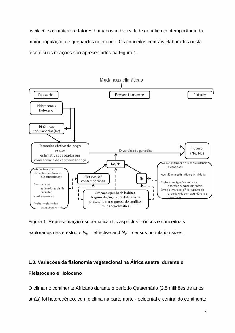
maior população de guepardos no mundo. Os conceitos centrais elaborados nesta
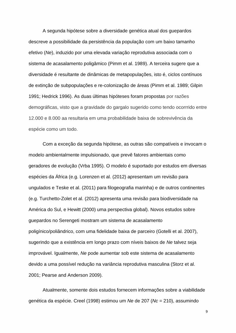
tese e suas relações são apresentados na Figura 1.
Figura 1. Representação esquemática dos aspectos teóricos e conceituais
explorados neste estudo. Ne = effective and Nc = census population sizes.
1.3. Variações da fisionomia vegetacional na África austral durante o
Pleistoceno e Holoceno
O clima no continente Africano durante o período Quaternário (2.5 milhões de anos
atrás) foi heterogêneo, com o clima na parte norte - ocidental e central do continente
5
tendo sido mais instável do que na região austral (Stokes et al. 1997; Dupont et al.
2008; Maslin et al. 2012). Mesmo considerada como tendo sido mais estável em
nível macro, oscilações no clima na África meridional foram notáveis em particular
durante o Pleistoceno e Holoceno (Chase et al. 2010; Weldeab et al. 2012). Pelos
menos quatro eventos periódicos de significante aridez são conhecidos durante o
Pleistoceno nos intervalos 135.000 ou 115.000 - 90.000 anos atrás (aa), 46.000 –
41.000 aa, 26.000 – 20.000 aa e 16.000 – 9.000 aa (Cohen et al. 2007; Stokes et al.
1997). Similarmente, registros indicam que o Último Máximo Glacial (UMG) (~
26.000 – 14.000 aa) (Feankins e deMenocal 2008; Clark et al. 2009) foi intercalado
possivelmente por condições úmidas (~ 27.000 – 22.000 aa e 19.000 – 12.000 aa)
(Thomas et al. 2003). Estudos mas recentes indicam pelos menos quatro fases
distintas úmidas do sul da África entre 8.500 e 3.500 aa, cada fase durando cerca
de 250 anos, e um aumento da aridez, desde então, até 300 anos atrás (Chase et
al. 2009). Em geral, o clima do Quaternário tornou-se progressivamente mais frio,
mais seco e sazonal (deMenocal 2004) mas às vezes regrediu e manteve-se estável
(de Vivo 2008). Associadas a essas alterações, ocorreram mudanças de paisagem
que conseqüentemente impactaram as linhagens de fauna e flora.
Durante este período, a vegetação do sul da África mudou, alternando
formas, mas progressivamente transicionando de florestas para ambientes abertos
(savanas). Estudos indicam um aumento significante de paisagens mais abertas
entre 1.8 Ma a 0.6 Ma (Cerling 1992; Bobe e Behrensmeyer 2004), com uma
progressão gradual de substituição de plantas adaptadas a condições úmidas por
plantas adaptadas a condições áridas (i.e. C4) (Dupont et al. 2008; Feakins e
deMenocal 2008). Paisagens dominadas por plantas C4 só foram estabelecidas em
torno de 1 Ma (Cerling 1992). Expansões de paisagens abertas ligadas a um
6
aumento da freqüência de secas e aridez também são registradas após 7.000 aa
(Dupont et al. 2008) ou 2.300 – 1.200 aa (Jolly et al. 1997). No entanto, há
evidências de contrações destas paisagens devido à expansão do deserto ao longo
dos últimos 10.000 anos (Hoelzmann et al. 1999; Osmers et al. 2012). Ligadas a
estas alterações de paisagens, houve diversas mudanças na composição da fauna.
A expansão de paisagens abertas resultou em uma substituição de
comunidades dominadas por herbívoros de grandes tamanhos corporais por
ungulados menores de pastagem (Ségalen et al. 2007; de Vivo 2008). O contrário
foi observado durante a transição Pleistoceno-Holoceno (18.000 – 12.000 aa), com
uma sobreposição de animais florestais e savânicos em vez de uma comunidade
primariamente composta de herbívoros de áreas abertas (Reed 1997; de Vivo 2008;
Faith 2012). Por exemplo, springbok Antidorcas springbok foi extinto no leste da
África (~ 400.000 anos atrás), mas não no sul da África, onde divergiram em duas
subespécies e recentemente recolonizaram o leste da África (Reynolds 2007).
Assim, além de algumas espécies se extinguirem, a distribuição de várias daquelas
que persistiram foi alterada. Por sua vez, estas mudanças afetaram os padrões de
persistência e distribuição dos carnívoros (Rohland et al. 2005; Cowling et al. 2007).
Bertola et al. (2011) indica que leões (Panthera leo) recolonizaram a parte oeste-
centro da África do Oriente Médio, após a população ter sido extinguida localmente
durante períodos de extrema aridez que levaram à redução de presas durante o
Pleistoceno.
Em suma, a África austral tem experimentado ciclos úmidos – secos de
diferentes durações, acompanhados por mudanças em habitat específicas para
cada espécie, cujas conseqüências incluem a extinção local ou regional, mudanças
7
na sua distribuição, e mesmo a formação de subespécies (e.g Johnston e Anthony
2012; Osmers et al. 2012).
1. 4 O status quo da história demográfica do guepardo
O guepardo, Acinonyx jubatus, é uma espécie ameaçada de extinção e classificada
como Vulnerável pela União Internacional para a Conservação da Natureza e
Recursos Naturais (IUCN), com menos de 12 mil indivíduos vivos na natureza,
distribuídos em 22 países (Durant et al. 2008). Esta distribuição representa 25% da
sua ocorrência histórica (Ray et al. 2005). Atualmente, com a exceção de Namíbia e
Botswana, as populações restantes são consideradas inviáveis, com populações
inferiores a 500 indivíduos (estimativas baseadas em suposições informadas
(Marker 1998; Durant et al. 2008). Com base nesta abordagem e em questionários,
a população de guepardos na Namibia é estimada de ser de 2.500 indivíduos
adultos, com um tamanho populacional (Nc) total estimado de 3.100 a 5.800
indivíduos (Hanssen e Stander 2004; Durant et al. 2008). No entanto, há uma
escassez de estimativas derivadas de estudos de médio-longo prazo, usando
métodos robustos e sistemáticos (e.g. Durant et al. 2011) Esta falta de estudos de
dinâmica populacional é parcialmente devida a aspectos ecológicos e
comportamentais da espécie (isto é, inconspícuas, noturnas, ocorrendo em baixa
densidade) (Gese 2001), que levam a uma necessidade de esforços de amostragem
maiores (Tomas e de Miranda 2003). Entretanto, tendências de abundância com
base em registros de animais removidos devido a conflito com humanos indicam um
declínio populacional ao longo do século passado (Marker-Kraus et al. 1996; Nowell
1996). Este declínio é resultado de razões ecológicas, incluindo secas, redução de
presas, perda e degradação de hábitat, bem como de caça troféus e remoções pelo
conflito real ou percebido com humanos (human-wildlife conflict -HWC) (O’Brien et
8
al. 1987; Marker Kraus et al. 1996; Nowell 1996; Marker et al. 2007). Na última
década, contudo, houve uma redução no número de indivíduos removidos, devido a
mudanças de manejo, e a população parece ter se estabilizado (Marker et al. 2007;
Castro-Prieto et al. 2011).
A origem da diversidade genética atual da espécie é resultado da
combinação de eventos anteriores à civilização moderna, em conjunto com fatores
antropogênicos ocorrendo em tempos recentes. Três hipóteses propostas resumem
esta combinação de fatores, embora elas ainda careçam de uma avaliação rigorosa
utilizando métodos estatísticos modernos. A primeira hipótese sugere um severo
gargalo genético em torno do fim do Último Máximo Glacial ou principio do Holocene
(12.000 - 8.000 aa), seguido por um período de endogamia intensa, uma expansão
em meados do Holoceno (5.000 anos) e finalmente um segundo gargalo durante o
ultimo século devido a fatores humanos e variabilidade climática (O’Brien et al.
1985, 1987; Menotti-Raymond e O’Brien 1994; Driscoll et al. 2002). Estas
conclusões são baseada no alto nível de homogeneidade detectado com vários
tipos de marcadores genéticos (isoenzimas, RFLPs [polimorfismos de comprimento
de fragmentos de restrição] de DNA mitocondrial [mtDNA], minissatélites,
microssatélites e variabilidade no Complexo Principal de Histocompatibilidade
[MHC]) em amostras da duas subespécies, A. j. jubatus e A.j. raineyi da África
Austral e Oriental, respectivamente (O’Brien et al. 1985, 1987; Menotti-Raymond e
O’Brien 1994). Estudos mas recentes, com maiores amostragens e cobertura
geográfica revelam níveis mais altos de diversidade para MHC, mtDNA e
microssatélites (Marker et al. 2008; Castro-Prieto et al. 2011; Charruau et al. 2011),
ainda que não contradigam claramente as inferências reportadas nos estudos
anteriores.
9
A segunda hipótese sobre a diversidade genética atual dos guepardos
descreve a possibilidade da persistência da população com um baixo tamanho
efetivo (Ne), induzido por uma elevada variação reprodutiva associada com o
sistema de acasalamento poligâmico (Pimm et al. 1989). A terceira sugere que a
diversidade é resultante de dinâmicas de metapopulações, isto é, ciclos contínuos
de extinção de subpopulações e re-colonização de áreas (Pimm et al. 1989; Gilpin
1991; Hedrick 1996). As duas últimas hipóteses foram propostas por razões
demográficas, visto que a gravidade do gargalo sugerido como tendo ocorrrido entre
12.000 e 8.000 aa resultaria em uma probabilidade baixa de sobrevivência da
espécie como um todo.
Com a exceção da segunda hipótese, as outras são compatíveis e invocam o
modelo ambientalmente impulsionado, que prevê fatores ambientais como
geradores de evolução (Vrba 1995). O modelo é suportado por estudos em diversas
espécies da África (e.g. Lorenzen et al. (2012) apresentam um revisão para
ungulados e Teske et al. (2011) para filogeografia marinha) e de outros continentes
(e.g. Turchetto-Zolet et al. (2012) apresenta uma revisão para biodiversidade na
América do Sul, e Hewitt (2000) uma perspectiva global). Novos estudos sobre
guepardos no Serengeti mostram um sistema de acasalamento
poligínico/poliândrico, com uma fidelidade baixa de parceiro (Gotelli et al. 2007),
sugerindo que a existência em longo prazo com níveis baixos de Ne talvez seja
improvável. Igualmente, Ne pode aumentar sob este sistema de acasalamento
devido a uma possível redução na variância reprodutiva masculina (Storz et al.
2001; Pearse and Anderson 2009).
Atualmente, somente dois estudos fornecem informações sobre a viabilidade
genética da espécie. Creel (1998) estimou um Ne de 207 (Nc = 210), assumindo
10
uma proporção sexual desviada pró-fêmeas (0,44: 0,56) e Ne 97 (Nc = 101) quando
incluiu indivíduos sem áreas próprias (‘transients”). Em contraste, Kelly (2001),
obteve valores de Ne < 50 usando quatro estimadores de Ne com diferentes
suposições, e não incluiu transientes. Além das diferenças nas estimativas, Creel
(1998) observou um efeito mínimo no Ne devido a flutuações no tamanho
populacional ou proporções sexual desiguais, dado não observado por Kelly (2001).
Como as estimativas de abundancia podem afetar o nível de impacto de flutuações
demográficas no valor calculado de Ne (Vucetich e Waite 1998), este fator pode
explicar a falta de influência para o caso de Creel (1998). A exclusão de transientes
por Kelly (2001) pode ter introduzido um viés negativo, considerando a infidelidade
de fêmeas (Gotelli et al. 2007). Contudo, ambos os estudos mostram que Ne é
afetado negativamente por sucessos reprodutivos desiguais. Esses dados reforçam
a necessidade de estudos semelhantes em outras populações.
1.6. Justificativas, e objetivos gerais e específicos do estudo
O estudo teve como objetivo geral a compreensão da demografia histórica e
contemporânea da população de guepardos da Namíbia ao longo dos últimos
60.000 anos, informações estas necessárias para a elaboração de estratégias
adequadas para sua conservação em longo prazo por três razões principais.
Primeiro, é necessária uma melhor compreensão dos processos históricos e
contemporâneos, como por exemplo, o impacto das oscilações climáticas do
Quaternário e fatores humanos que moldaram e possivelmente continuam a
influenciar a diversidade genética contemporânea desta população.
Segundo, a população de guepardos da África austral, e da Namíbia em
particular, representam a maior população natural desta espécie no mundo (Durant
11
et al. 2008; Marker et al. 2010) e tem uma diversidade genética maior do que as
outras populações (Charrua et al. 2011). Além disso, aparenta comportar-se como
uma população panmítica em escala nacional (Marker et al. 2008). No entanto, Ne é
frequentemente menor que Nc e da proporção de indivíduos reprodutores breeding
proportions (Nb) (Frankam 1995; Vucetich e Waite 1998; Palstra e Ruzzante 2008;
Palstra e Fraser 2012), mesmo em populações grandes (Palstra e Fraser 2012),
podendo assim ocasionar uma tendência à perda de variabilidade e menor
viabilidade em longo prazo por influência da deriva genética (Hare et al. 2011).
Finalmente, uma compreensão dos processos que regem a dinâmica
genética (Ne) e demográfica é necessária principalmente para espécies ou
populações em conflito com humanos (Lucherini e Merino 2008; Marker et al. 2010).
A redução de indivíduos adultos na população afeta o tamanho de censo e tem o
potencial de afetar diretamente a diversidade genética da população (Saether et al.
2009; Palstra e Ruzzante 2010; Lee et al. 2011).
De forma geral, a escassez de estudos sobre tamanhos efetivos históricos e
contemporâneos, bem como sobre a dinâmica populacional. Isto limita uma
compreensão dos fatores afetando a diversidade genética das populações e da
espécie.
1.6.1. Objetivos gerais e específicos
Para atingir a meta principal de obter uma compreensão mais ampla sobre os
processos que moldam a diversidade genética da espécie, foram delimitados três
objetivos específicos, sendo eles: (1) uma avaliação estatística da história
demográfica da espécie em relação à variabilidade climática do Quarternário e a
fatores antropogênicos; (2) uma investigação da interação entre o seu tamanho
12
populacional efetivo contemporâneoe e suas taxas vitais; e (3) uma avaliação
aprofundada de tendências de abundância e densidade.
1.7. Ferramentas de estudo
Para explorar a história demográfica de guepardos durante os últimos 60.000 anos,
utilizou-se o método Bayesiano de computação aproximada (ABC) (Storz et al.
2002; Lopes e Beaumont 2010) implementada no pacote DIYABC-FDA (Cornuet et
al. 2010, 2008; Estoup et al. 2012). Este período foi estratificado a fim de avaliar
correlações entre oscilações climáticas e/ou fatores antropogênicos com mudanças
demográficas em escalas menores de tempo. Mudanças demográficas anteriores a
1.000 aa foram interpretadas como sendo relacionadas às oscilações climáticas, e
aquelas com idade de 1.000 aa ou menos como sendo um efeito combinado com
fatores antropogênicos. Em essência, a análise de ABC utiliza uma matriz
coalescente de verossimilhança, gerando um grande número de amostras por meio
de simulações de Monte Carlo, e aplica estatísticas sumárias para selecionar os
conjuntos de dados mais próximos ao conjunto de dados real ) (Excoffier et al. 2005;
Lopes e Beaumont 2010). Em seguida, baseando-se nos conjuntos de dados mais
próximos, a probabilidade relativa posterior de diferentes modelos é calculada,
incluindo inferências de parâmetros demográficos associados.
Para avaliar a sensibilidade da estimativa de viabilidade populacional a
perturbações nas taxas vitais, bem como a incertezas no tamanho da população e
na capacidade suporte, foram realizadas análises de sensibilidade utilizando-se o
programa VORTEX, um software de análise de viabilidade que integra vários
aspectos da história de vida da população (Miller e Lacy 2005). Três métodos foram
utilizados para determinar o tamanho contemporâneo efetivo da população: (i) o
13
método coalescente ABC implementado no programa ONeSAMP (Tallmon et al.
2008); e (ii) método de desequilíbrio de ligação implementado no programa LDNe
(Waples 2006; Waples e Do 2010); e (iii) utilizando as simulações demográficas
realizadas com o programa VORTEX e a fórmula Ne = ½ (1 - exp (logeHt / t)), onde Ht é
a heterozigosidade esperada após os processos simulados (Crow e Kimura 1970,
ver Eizirik et al. [2002] para uma aplicação).
Por fim, para avaliar as tendências em densidade e abundância em uma
população local de guepardos, métodos espaciais de captura-recaptura (Royle et al.
2009) foram aplicados, utilizando o software SPACECAP (Gopalaswamy et al.
2012). Estes foram baseados em um conjunto de dados de uma área de tamanho
similar amostrada por seis anos com armadilhas fotográficas colocadas, na maior
parte, em sítios de marcação. Padrões de utilização de áreas, marcação, e
fidelidade em relação a áreas de permanência também foram explorados.
Referências
Bertola LD, Van Hooft WF, Vrieling K, Uit de Weerd DR, York DS, Bauer H, Prins
HHT et al. (2011) Genetic diversity, evolutionary history and implications for
conservation of the lion (Panthera leo) in West and Central Africa. J Biogeogr 38
1356–1367.
Bobe R, Behrensmeyer AK (2004) The expansion of grassland ecosystems in Africa
in relation to mammalian evolution and the origin of the genus Homo.
Palaeogeogr Palaeoclimatol Palaeoecol 207: 399–420.
Caughley G, Gunn A (1996) Conservation biology in theory and practice.
Blackwell Science, New York
14
Castro-Prieto A, Wachter B, Sommer S (2011) Cheetah paradigm revisited: MHC
diversity in the world’s largest free-ranging population. Mol Biol Evol 28: 1455 –
1468
Cerling TE(1992) Development of grasslands and savannas in East Africa during the
Neogene. Palaeogeogr Palaeoclimatol Palaeoecol 97: 241–247
Charruau P, Fernandes C, Wengel PO, Peters J, Hunter L, Ziaie H, Jourabchian A,
et al (2011) Phylogeography , genetic structure and population divergence time
of cheetahs in Africa and Asia : evidence for long-term geographic isolates. Mol
Ecol 20:, 706–724
Chase BM, Meadows ME, Carr AS, Reimer PJ (2010) Evidence for progressive
Holocene aridification in southern Africa recorded in Namibian hyrax middens:
Implications for African Monsoon dynamics and the “‘African Humid Period’”.
Quatern Res 74: 36–45
Chase BM, Meadows ME, Scott L, Thomas DSG, Marais E, Sealy J, Reimer PJ
(2009) A record of rapid Holocene climate change preserved in hyrax middens
from southwestern Africa. Geology 37: 703–706
Clark PU, Dyke AS, Shakun JD, Carlson AE, Clark J, Wohlfarth B, Mitrovica JX, et al
(2009) The Last Glacial Maximum. Science 325: 710–4
Cohen AS, Stone JR, Beuning KRM, Park LE, Reinthal PN, Dettman D, Scholz CAet
al (2007) Ecological consequences of early Late Pleistocene megadroughts in
tropical Africa. PNAS 6–11
15
Cornuet J-M, Ravigné V, Estoup A (2010) Inference on population history and model
checking using DNA sequence and microsatellite data with the software
DIYABC (v1.0). Bioinformatics 11, 401. doi:10.1186/1471-2105-11-401
Cornuet J-M, Santos F, Beaumont MA, Robert CP, Marin J-M, Balding DJ,
Guillemaud T, T., et al (2008) Inferring population history with DIY ABC: a user-
friendly approach to approximate Bayesian computation. Bioinformatics 24:
2713–9
Cowling SA, Cox PM, Jones CD, Maslin MA, Peros M, Spall SA (2008) Simulated
glacial and interglacial vegetation across Africa: implications for species
phylogenies and trans-African migration of plants and animals. Global Change
Biol 14: 827–840.
Creel S (1998) Social organization and effective population size in carnivores. In:
Caro T (ed) Behavioral ecology and Conservation biology. Oxford University Press,
New York, pp 246–270
Crow JF, Kimura AM (1970) An introduction to population genetics theory. Harper &
Row, Publishers, London
deMenocal PB (2004) African climate change and faunal evolution during the
Pliocene–Pleistocene. Earth Planet. Sci. Lett 220: 3–24
de Vivo, M. (2008). Mamíferos e mudanças climáticas. In: Buckeridge MS
(ed) Biologia e Mudanças Climáticas no Brasil. São Carlos, Editora Rima, pp.
207-223
16
Driscoll CA, Menotti-Raymond M, Nelson G, Goldstein D, O’Brien SJ (2002)
Genomic microsatellites as evolutionary chronometers: a test in wild cats.
Genome Res 12: 414–23
Dupont LM, Behling H, Kim J-H (2008) Thirty thousand years of vegetation
development and climate change in Angola (Ocean Drilling Program Site 1078).
Clim Past 4: 111–147
Durant SM, Craft ME, Hilborn R, Bashir S, Hando J, Thomas L (2011) Long-term
trends in carnivore abundance using distance sampling in Serengeti National
Park, Tanzania. J Appl Ecolo 48: 1490–1500
Durant S, Marker L, Purchase N, Belbachir F, Hunter L, Packer C,
Breitenmoser-Wursten C, Sogbohossou E, Bauer H (2008) Acinonyx jubatus.
In: IUCN 2012. IUCN Red List of Threatened Species. Version 2012.2.
<www.iucnredlist.org>. Downloaded on 10 March 2012
Eizirik E, Indrusiak CB, Johnson WE (2002) Jaguar population viability analysis:
Evaluation of parameters and case-studies in three remnant populations of
southern South America. In: Medellín AR, Chetkiewicz C, Rabinowitz A, Redford
KH, Robinson JG, Sanderson E, Taber A (eds). Jaguars in the new millenium: a
status assessment, priority detection, and recommendations for the
conservation of jaguars in the Americas. Universidad Nacional Autonoma de
Mexico, Mexio and Wildlife Conservation Society, USA, pp 1–20
Estoup A, Lombaert E, Marin J, Guillemaud T, Robert CP, Cornuet J, Antipolis DN,
et al (2012) Estimation of demo-genetic model probabilities with Approximate
17
Bayesian Computation using linear discriminant analysis on summary statistics.
Mol Ecol Resour 12: 846–855
Excoffier L, Estoup A, Cornuet J (2005) Bayesian Analysis of an Admixture Model
with Mutations and Arbitrarily Linked Markers. Genetics 1738: 1727–1738
Frankham R (1995) Effective population size/ adult population size ratios in wildlife.
Genet Res 66: 95-107
Faith JT (2012) Palaeozoological insights into management options for a threatened
mammal: southern Africa’s Cape mountain zebra (Equus zebra zebra). Divers
Distrib18: 438–447
Feankins s, DeMenocal P (2008) Global and African Regional Climate during the
Cenozoic. In Werdelin L, Sanders W (eds) Cenozoic Mammals in Africa.
University California Press, USA, pp 45–56
Fraser CI, Nikula R, Ruzzante DE, Waters JM (2012) Poleward bound: biological
impacts of Southern Hemisphere glaciation. TREE 27: 462–71
Gese EM (2001) Monitoring of terrestrial carnivore populations. In: Gittleman JL,
Funk SM, MacDonald DW (eds) Carnivore Conservation. Cambridge University
Press, UK, pp 372 - 396
Gilpin M (1991) The genetic effective size. Biol J Linn Soc 42: 165–175
Gopalaswamy AM, Royle JA, Hines JE, Jathanna D, Kumar NS, Karanth KU (2012)
A program to estimate animal abundance and density using Bayesian spatially-
18
explicit capture recatpure models. Package “ SPACECAP ”. Retrieved from
http://cran.r-project.org/web/packages/SPACECAP/index.html
Gottelli D, Wang J, Bashir S, Durant SM (2007) Genetic analysis reveals promiscuity
among female cheetahs. Proc R Soc B 274: 1993–2001
Hanssen L, Stander P (2004) Namibia large carnivore atlas. Predator Conservation
Trust, Windhoek. Windhoek, Namibia, pp 1–12
Hare MP, Nunney L, Schwartz MK, Ruzzante DE, Burford M, Waples RS, Ruegg K,
Palstra F (2011) Understanding and Estimating Effective Population Size for
Practical Application in Marine Species Management. Conserv Biol 1–12
doi:10.1111/j.1523-1739.2010.01637.x
Hedrick PW (1996) Bottleneck (s) in Cheetahs or Metapopulation. Conserv Biol 10:
897–899
Hewitt G (2000) The genetic legacy of the Quaternary ice ages. Nature 405:907–13
Hewitt G (2004) Genetic consequences of climatic oscillations in the Quaternary. Phil
Trans R Soc B 359: 183–195
Hoelzmann P, Jolly D, Harrison SP, Laarif F, Bonnefille R (1998) Mid-Holocene land-
surface conditions in northern Africa and theArabian peninsula : A data set for
the analysis of biogeophysical feedbacks in the climate system. Global
Biogeochemical Cycles 12: 35–51
Holt RD (1990) The microevolutionary consequences of climate change. TREE 5:
311–5
19
Johnston AR, Anthony NM (2012) A multi-locus species phylogeny of African forest
duikers in the subfamily Cephalophinae: evidence for a recent radiation in the
Pleistocene. J Evolution Biol doi:10.1186/1471-2148-12-120
Jolly D, Taylor D, Marchant R, Hamilton A, Bonnefille R, Buchet G, Riollet G (1997)
Vegetation dynamics in central Africa since 18,000 yr BP : pollen records from
the interlacustrine highlands of Burundi , Rwanda and western Uganda. J
Biogeogr 24: 495–512
Kelly MJ (2001) Lineage Loss in Serengeti Cheetahs: Consequences of High
Reproductive Variance and Heritability of Fitness on Effective Population Size.
Conserv Biol 15: 137–147
Kharouba HM, Mccune JL, Thuiller W, Huntley B (2012) Do ecological differences
between taxonomic groups influence the relationship between species ’
distributions and climate? A global meta-analysis using species distribution
models. Ecography 35: 1–8 doi:10.1111/j.1600-0587.2012.07683.x
Lee AM, Engen S, Sæther B (2011) The influence of persistent individual differences
and age at maturity on effective population size Subject collections: Proc R Soc
B doi:10.1098/rspb.2011.0283
Lopes JS, Beaumont MA (2010) ABC: a useful Bayesian tool for the analysis of
population data. Infect Genet Evol 10: 826–833
LorenzenED, Heller R, Siegismund HR (2012) Comparative phylogeography of
African savannah. Mol Ecol 21: 3656–3670.
20
Lorenzen ED, Nogués-Bravo D, Orlando L, Weinstock J, Binladen J, Marske KA,
Ugan A, et al (2011) Species-specific responses of Late Quaternary megafauna
to climate and humans. Nature 479: 359–64
Lucherini M, Merino MJ (2008) Perceptions of Human–Carnivore Conflicts in the
High Andes of Argentina. Mt Res Dev 28: 81–85. doi:10.1659/mrd.0903
Marker LL (1998) Current Status of the cheetah (Acinonyx jubatus). Proceedig of a
Symposium on Cheetahs as Game Ranch Animals. South Africa, pp 1 – 17
Marker-Kraus L, Kraus D, Barnett D. Hurlbut S (1996) Cheetah survival on
Namibian farmlands. Cheetah Conservation Fund, Windhoek.
Marker LL, DickmanAJ, Mills MGL, Macdonald DW (2010) Cheetahs and ranchers in
Namibia : a case study. In: MacDonald D, Loveridge A (eds) Biology and
Conservation of Wild Felids. Oxford University Press, UK, pp 353 – 372
Marker LL, Dickman AJ, Wilkinson C, Schumann B, Fabiano E (2007) The Namibian
Cheetah : Status Report. Cat News, Special Issue 3: 4–13
Marker LL, Wilkerson AJP, Sarno RJ, Marteson J, Breitenmoser-Würsten C, O’Brien
SJ, Johnson WE (2008) Molecular Genetic Insights on Cheetah (Acinonyx
jubatus) Ecology and Conservation in Namibia. J Hered 99: 2–13
Maslin MA, Pancost RD, Wilson KE, Lewis J, Trauth MH (2012) Three and half
million year history of moisture availability of South West Africa : Evidence from
ODP site 1085 biomarker records. Palaeogeogr Palaeoclimatol Palaeoecol 317-
318: 41–47
21
Menotti-Raymond MA, O’Brien SJ (1994) Evolutionary conservation of ten
microsatellite loci in four species of Felidae. J Hered 86: 319–22
Miller PS, Lacy RC (2005) VORTEX A stochastic simulation of the extinction process
V 9.50. Apple Valley: Conservation Breeding Specialist Group (SSC/IUCN)
Nowell K (1996) Namibian Cheetah Conservation Strategy. Windhoek, Namibia, pp1
– 41O’Brien SJ, Roelke ME, Marker LL, Newman A, Winkler CA, Meltzer D,
Colly L, Evermann JF, Bush M, Wildt, DE (1985). Genetic basis for species
vulnerability in the cheetah. Science 227: 1428–34O’Brien SJ, Wildt DE, Bush
M, Caro TM, FitzGibbon C, Aggundey I, Leakey RE (1987) East African
cheetahs: evidence for two population bottlenecks? PNAS 84: 508–11
Osmers B, Petersen B, Hartl GB, Grobler JP, Kotze A, Aswegen E Van, Zachos FE
(2012) Genetic analysis of southern African gemsbok (Oryx gazella) reveals
high variability, distinct lineages and strong divergence from the East African
Oryx beisa. Mamm Biol 77: 60–66
Palstra FP, Fraser DJ (2012) Effective/census population size ratio estimation: a
compendium and appraisal. Ecology and Evolution 2: 2357–65
doi:10.1002/ece3.329
Palstra FP, Ruzzante DE (2008) Genetic estimates of contemporary effective
population size : what can they tell us about the importance of genetic
stochasticity for wild population persistence? Mol Ecol 17: 3428–3447
Pearse DE, Anderson EC (2009) Multiple paternity increases effective population
size. Mol Ecol 18: 3124–3127
22
Phillips CD, Hoffman JI, George JC, Suydam RS, Huebinger RM, Patton JC,
Bickham JW (2012) Molecular insights into the historic demography of bowhead
whales: understanding the evolutionary basis of contemporary management
practices. Ecology and Evolution 3: 18–37 Pimm SL, Gittleman JL, McCracken
GF, Gilpin M (1989) Plausible alternatives to bottlenecks to explain reduced
genetic diversity. TREE 4: 176 – 178
Ray JC, Hunter L, Zigouris J (2005) Setting conservation and research priorities for
larger African carnivores setting conservation for larger African. WCS Working
Paper No. 24. Wildlife Conservation Society, New York, pp 1 - 201
Reed KE (1997) Early hominid evolution and ecological. J Hum Evol 32: 289 – 322
Reynolds SC (2007) Mammalian body size changes and Plio-Pleistocene
environmental shifts: implications for understanding hominin evolution in eastern
and southern Africa. J Hum Evol 53, 528–48
Rohland N, Pollack JL, Nagel D, Beauval C, Airvaux J, Pääbo S, Hofreiter M (2005)
The population history of extant and extinct hyenas. Mol Biol Evol 22: 2435–43
Royle JA, Karanth KU, Gopalaswamy AM, Kumar NS (2009) Bayesian inference in
camera trapping studies for a class of spatial capture-recapture models. Ecology
90: 3233–44
Saether BE, Engen S, Solberg EJ (2009) Effective size of harvested ungulate
populations. Anim Conserv 12: 488–495
Ségalen L, Lee-Thorp JA, Cerling T (2007) Timing of C4 grass expansion across
sub-Saharan Africa. J Hum Evol 53: 549–59
23
Stokes S, Thomas DSG, Washington R (1997) Multiple episodes of aridity in
southern Africa since the last interglacial period. Nature 388: 2–6
Storz JF, Ramakrishnan U Alberts SC (2001) Determinants of Effective Population
Size for Loci with Different Modes of Inheritance. J Hered 92: 497–502.
Storz JF, Beaumont MA, Alberts SC (2002) Genetic evidence for long-term
population decline in a savannah-dwelling primate: inferences from a
hierarchical bayesian model. Mol Biol Evol 19: 1981–90
Tallmon DA, Koyuk A, Luikart G, Beaumont MA (2008) ONeSAMP : a program to
estimate effective population size using approximate Bayesian computation. Mol
Ecol Resour 8: 299–301
Teske P, Heyden S von der, McQuaid CD, Barker NP (2011) A review of marine
phylogeography in southern Africa Coastal phylogeography. S Afr J Sci 107: 1–
11
Thomas D, Brook G, Shaw P, Bateman M, Haberyan K, Appleton C, Nash D,
McLaren S, Davies F (2003) Late Pleistocene wetting and drying in the NW
Kalahari: an integrated study from the Tsodilo Hills, Botswana. Quatern Int 104:
53 – 67
Tomas WM, Miranda GHB (2003) Uso de armadilhas fotográficas em levantamentos
populacionais. In: Cullen L Jr; Rudran R, Valladares-Padua C (eds) Métodos de
estudo em biologia da conservação e manejo da vida silvestre. Curitiba, Editora
UFPR, pp 243-267
24
Turchetto-Zolet AC,, Pinheiro F, Salgueiro F, Palma-Silva C (2012)
Phylogeographical patterns shed light on evolutionary process in South
America. Mol Ecol doi:10.1111/mec.12164
Vasemägi A, Palstra FP, Ruzzante DE (2010) A temporal perspective on population
structure and gene flow in Atlantic salmon (Salmo salar) in Newfoundland,
Canada. Can J Fish Aquat Sci 67: 225–242
Vrba ES (1995) The fossil record of African antelopes (Mammalia, Bovidae) in
relation to human evolution and paleoclimate. In Vrba ES, Denton GH,
Partridge TC, Burckle LH (eds) Paleoclimate and evolution, with emphasis on
human origins. Yale University Press, New Haven, CT, pp 385–424
Vucetich JA Waite TA (1998) Number Estimation of Censuses of Required for
Demographic Effective Population Size. Conserv Biol 12: 1023–1030
Waples RS (2006) A bias correction for estimates of effective population size based
on linkage disequilibrium at unlinked gene loci. Conserv Gen 7: 167–184
Waples RS Do C (2010) Linkage disequilibrium estimates of contemporary Ne using
highly variable genetic markers: a largely untapped resource for applied
conservation and evolution. Evolutionary Applications 3: 244–262
Weir JT Schluter D (2007) The latitudinal gradient in recent speciation and extinction
rates of birds and mammals. Science 315: 1574–6
Weldeab S, Stuut JW, Schneider RR, Siebel W (2012) Holocene climate variability in
the winter rainfall zone of South Africa. Clim Past 2281–2320

25

26
Capitulo II
27
Inferring the historical demography of the Namibian cheetah population using
Bayesian analysis of microsatellite data
Authors:
Mr. Ezequiel Chimbioputo Fabiano, a, b
Dr. Sandro Luis Bonatto, PhD, a
Dr. Anne Schmidt-Küntzel, PhD, DMV, b, c
Dr. Laurie L. Marker, PhD, b
Prof. Eduardo Eizirik, PhD, a
Email addresses:
[email protected], [email protected]
Affiliations:
a. Laboratório de Biologia Genômica e Molecular, Faculdade de Biociências,
Pontifícia Universidade Católica do Rio Grande do Sul, Porto Alegre, RS 90619-900,
Brazil
28
b. Cheetah Conservation Fund, PO Box 1755, Otjiwarongo, Namibia.
c. Life Technologies Conservation Genetics Laboratory, Cheetah Conservation
Fund, PO Box 1755, Otjiwarongo, Namibia.
Corresponding author:
Mr. Ezequiel Chimbioputo Fabiano, Laboratório de Biologia Genômica e Molecular,
Faculdade de Biociências, Pontifícia Universidade Católica do Rio Grande do Sul,
Porto Alegre, RS 90619-900, Brazil; Cheetah Conservation Fund, Otjiwarongo,
Namibia.
Email: [email protected]
Prof. Eduardo Eizirik, Laboratório de Biologia Genômica e Molecular, Faculdade de
Biociências, Pontifícia Universidade Católica do Rio Grande do Sul, Porto Alegre,
RS 90619-900, Brazil
Email: [email protected]
29
Abstract
The contemporary genetic diversity of the cheetah (Acinonyx jubatus) has been the
focus of several studies over the last 25 years, most of which have revealed low
levels of variation at genomic and mitochondrial markers. Such low variation has
been suggested to derive from two historical genetic bottlenecks, a severe one at the
end of the Last Glacial Maximum (LGM) and a more recent one in the past
millennium, with a possible expansion during the mid-Holocene (~ 5000 years ago
[ya]). Here, we used approximate Bayesian computation (ABC) methods with
temporal stratification to explore the historical demography of the largest free-
ranging cheetah population for the past 60,000 years. Results indicate that the
population has been declining gradually, interrupted by periods of stability. The
timing of the declines coincides with climatic events including over the last 3,500 -
300 ya, throughout the Holocene (~8,000 – 3,500 ya) and the late end of the LGM
and early half of the Holocene (~14,400 to 8,000 ya). Prior to 21,000 ya the
population appears to have been stable. These results demonstrate the impact of
slow contractions likely induced by the direct and indirect effects of climatic
oscillations in this population genetic diversity. This phenomenon is also relevant to
other species threatened with extinction due to slow loss of habitat ranges.
30
Introduction
Throughout the Quaternary period (which began 2.5 million years ago [Mya]), the
climate was highly heterogeneous in Africa, with western and eastern Africa’s
climate being more unstable than that of southern Africa [1, 2]. Despite southern
Africa’s relative climatic stability over the past 3.5 million years [3], notable
oscillations have been reported [4]. The climate in this region oscillated between wet
and dry periods [5], accompanied by changes on species-specific habitat suitability
[1, 2, 6-8]. This heterogeneity in climate has affected the contemporary genetic
diversity of many species, with comparative phylogeography across taxa indicating
southern Africa as a refugium from which populations recolonized more northerly
regions [9-11]. Since responses can be species- or population-specific [12],
reconstructing comparative historical patterns requires in-depth studies of many
taxa.
One species that seems to have a particularly interesting demographic history
is the cheetah (Acinonyx jubatus), for which several population genetic studies have
revealed remarkably low levels of genetic diversity [13,14]. Namibia has the largest
cheetah population, estimated at 2500 adult individuals [15] or a total census
population size of 3100 to 5800 individuals [16]. Botswana and South Africa in
southern Africa and Kenya and Tanzania in East Africa population sizes range
between 500 to 1500 individuals [15]. The remaining 18 population estimates are
bbelow 500 individuals [17] and are considered non-viable [18]. Records indicate
that the Namibian population has declined over the last century due to various
factors, including droughts, reduction in prey availability, habitat loss and
degradation, as well as trophy hunting and human-wildlife conflict [19-21]. However,
the population is considered to have stabilized in the recent decade [21].
31
While it is widely recognized that the origin of the cheetah’s relatively low
extant genetic diversity is the result of events pre-dating modern civilization, possibly
in combination with human-related factors, the exact mechanism that led to this
observed pattern is unknown. Three hypotheses corresponding to different patterns
of reduction in population size have so far been proposed to account for the species’
low level of genetic variation. Early population genetic studies using a variety of
genetic markers (allozymes, MHC variation, mtDNA restriction fragment length
polymorphisms and microsatellites) and samples from the southern and eastern
African subspecies, A. j. jubatus and A.j. raineyi, respectively, revealed high levels of
homogeneity [13, 14, 22 -24]. These studies proposed that the low diversity was
likely a consequence of a severe bottleneck at the end of the Pleistocene (12,000 -
10,000 years ago [ya]), followed by an expansion ca. 5,000 ya and another decline
within the past century. Two alternative hypotheses were subsequently proposed for
the genetic uniformity. First, that the species persisted at low effective population
size (Ne) induced by the high reproductive variance observed in species with a
polygynous mating system [25]. Second, that populations were subjected to a
continuous cycle of extinction of subpopulations followed by re-colonization of the
areas,following metapopulation dynamics [25-27]. While additional investigation is
required to resolve the debate, all three hypotheses are to some extent non-
exclusive, and imply an environmentally driven model [28], which postulates
environmental factors as drivers of evolution. This model has been supported in a
number of species worldwide [4,6], as well as more specifically in Africa and
southern Africa [29–31].
Since the publication of the classical studies on cheetah genetics, and in
particular during the past decades, there has been a surge of advances in
32
computational methods for exploring the historical demography of any organism
using empirically collected molecular data. Of particular interest is the application of
Approximate Bayesian Computation (ABC) approaches to population genetics
[32,33]. These methods have now been widely used to investigate the demographic
history of many different species, allowing the statistical comparison of contrasting
models of past population changes[e.g. 34–37].
Here we explored the demographic history of the Namibian cheetah
population using ABC methods, based on a previously published microsatellite data
set [37]. This population was considered appropriate for the study due to the
availability of a suitable genetic data set, the population having a large census size
[17] and being panmictic [37]. The latter is crucial, as it reduces the risk of false
signals of bottleneck caused by sub-structuring [38,39] while large sizes reduce the
likelihood of the population having experienced high genetic drift in the recent past
[40]. We specifically assessed whether the population has remained stable, declined
(gradually or severely) or expanded over different historical periods encompassing
subspecies divergence times and major climatic events (< 60,000 ya). This study is
timely, as a better understanding of this population’s demographic history is vital for
the development of effective conservation measures on its behalf.
Material and Methods
Data collection
To investigate the demographic history of Namibian cheetahs, we used a previously
published data set comprising 90 individuals genotyped for 31 dinucleotide
33
microsatellite loci [37]. This particular subset of the original data was composed only
of unrelated cheetahs, determined based on behavioural data, parentage analyses
and confirmed with estimates of genetic relatedness. For a full description of data
collection, see [37].
Past demographic analysis
We used the coalescence-based approach implemented in the program DIYABC-
FDA (hereafter DIYABC) [43-45]. This approach is based on the Wright-Fisher
model, and hence assumes that the study population approximates this model
[95,96].
DIYABC allows for the simulation, comparison and confidence assessment of
model choices considering more complex evolutionary scenarios [44]. It implements
a linear discriminant analysis (LDA) on summary statistics (Ss) prior to computing
posterior probabilities or evaluating confidence in scenario choice, as a means of
reducing computation time [44,45]. Ultimately, this gain in computation time allows
for additional simulations, thus partially overcoming a drawback concerning model
discrimination [50]. We assessed whether the population was stable, declined
(gradually or severely) or expanded over different timeframes that ranged from very
recent (120 to 6 ya) to ancestral (60,000 ya) times (Fig. 1, Table 1). The timeframes
were set so as to include subspecies divergence time estimates, climatic oscillations
and anthropogenic factors (Table S1). We grouped models into three main
categories, with each category corresponding to a discrete period (Table 1).
Category one encompassed recent (< 1,000 ya) and category 2 ancestral (> 1,000
ya) timeframes, while category 3 encompassed both, recent and ancestral
timeframes (Table 1). We attributed any demographic change occurring more than
34
1,000 ya as linked to climatic oscillations, while more recent changes were attributed
to anthropogenic influences with (1,000 ya to 300 ya) or without (300 ya to present)
climatic factors. This temporal stratification allowed for an assessment at a finer
temporal resolution than DIYABC assuming Ne to be constant between time periods
[44]. As part of category three we assessed robustness of model inference by
performing three additional runs whose times of decline encompassed most of the
multiple fine-scale periods (i.e. models 8 - 10, Table 1). In order to convert time of
change into years (T) and due to uncertainty in the cheetah’s mean generation time,
we considered estimates of 2.4 years [46,47], 4.05 years (Fabiano et al. unpublished
data [Chapter 3]) and 6 years [48]. The first value is based on long-term monitoring
data for females, the second derives from VORTEX simulations that incorporate life
history parameters and the third from data of captive animals at zoological
institutions.
Priors for ancestral effective population size (Nanc) were vague due to a lack of
records prior to the 1970's [19]. For the recent Ne (Nrec), we used "uninformative"
priors based on our parallel work (Chapter 3), and population size estimates of 2,500
adult individuals [17] or a total population size of 3,138 to 5,775 [37]. Hence, priors
for Nrec overlapped across scenarios (Table S2). As we were also interested in the
magnitude of the decline(s), we confined the upper and lower bound of the Nrec and
Nanc to differ by less than 5% (less severe) and at least by 50% (severe),
respectively, for five scenarios (Table 1, S2). Demographic parameters were
sampled from a uniform distribution (U). Microsatellite loci were assumed to follow
the generalized stepwise mutation model, with mutational parameters kept at the
default values (Table S2) [73–75]. Default priors for the mean and individual locus
mutation rates encompassed rates previously used for cheetahs (2.05 X 10⁻³, 5.6 X
35
10-4, 2.05 X 10⁻⁴) [51]. We also assessed the impact of using a broader prior for the
geometric distribution (P) U ~ [0.1 - 0.3] to U ~ [0.1 - 0.7] [52] with longer timeframe
periods (240,000 ya) on model selection (Table S3). This accounted for the
uncertainties in mutation rates of dinucleotide microsatellites in the context of model
selection [52,53].
Confidence on model choice: For each model, we performed 5 X 10⁵ simulations
of which 1% were selected based on the closest Euclidean distance between their
Ss and the Ss derived from the actual data for model checking, comparison and
parameter estimation [43]. We used as Ss the mean number of alleles, genic
diversity, variance in allele size in base pairs and Garza-Williamson's MWG [44,45].
The posterior probabilities of different scenarios were then computed using a
polychotomous logistic regression based on (K- 1) discriminant variables determined
by applying a linear discriminating analysis on the Ss of the closest simulated data
sets [45]. As the K-1 discriminant variables maximize differences among scenarios,
they provided an assessment of model discrimination. In addition, following Cornuet
et al. (2008) [44], we computed type I and II errors based on 500 simulated data
sets, as a means of discriminating among scenarios. Specifically, we estimated type
I error as the number of instances a scenario used to generate the data did not
exhibit the highest posterior probability (HPP) among the competing scenarios, and
type II error (β) as the proportion of times when a scenario had the HPP when the
data had actually been simulated under a competing scenario (i.e. statistical power =
1 - β). Additionally, we assessed the predictive power of different scenarios by
conducting a principal component analysis (PCA) on Ss derived from 1000 records
drawn from the posterior distribution, and visually inspected whether the observed
36
data set fell within the simulated data set with initial priors [45]. The lack of low tail
probabilities was also used as evidence of model fit [44].
Parameter estimation: The closest data sets (1% of simulated data sets), were then
used to calculate posterior probabilities of each scenario, upon which point estimates
with 95% HPD were determined using a logistic regression [44]. Point estimates
were present along the 95% HPD, with the relative mean square error (RRMSE),
bias and factor 2 used as measures of precision. Additionally, we report the posterior
distribution 50% and 95% coverage, and the mean integrated squared error
(RRMISE). The RRMISE was used as the optimizer criteria for parameter estimates
[54].
RESULTS
Single demographic changes
To assess whether and how the population size has changed over time, we
evaluated seven time periods for three to four scenarios each, assuming a single
demographic change (stable, gradual or severe declining, or expanding population)
(Table 1). The stable scenario unequivocally had the highest posterior probability
(HPP) in three timeframes, in three timeframes the stable and declining scenarios
were equally probable (their 95% HPP overlapped) and in one timeframe the
declining scenario had the HPP. In no instance did a scenario assuming an
expansion have a relative HPP, nor was it equally probable to another scenario
(Table 1). These findings suggest that, except, for a decline between 14,400 and 300
ya, and possibly between 40,000 and 30,000 ya, the population was more likely to
have been stable over most of the timeframes assessed. It is noteworthy that severe
declines were the least supported for time periods assessed for this scenario
37
(models 3, 4, 6, 7 in Table 1). Confidence in scenario choices was high, as statistical
power among the competing best scenarios was on average 80% (S2 Table 4).
Furthermore, none of the test statistics used to assess model misfit had a low tail
probability, suggesting that models did fit the data (i.e. probabilities were within 0,05
- 0,95 interval, S2 Table 5).
A congruent interpretation of the population history was also recovered based
on simulations characterized by broader priors for the time of change (models 8 - 10,
Table 1) (S2 Table 3, 4, 6). Under the broadest prior distribution that encompassed
all temporal periods (60,000 to 10 ya), the stable and decline scenarios were equally
probable (95% HPP range 0.4233 - 0.4722). A signal of decline was recovered with
model nine (T set to 12,000 to 3,000 ya) keeping largely in agreement with
conclusion of model three and a partly with models two and four (Table 1). Lastly,
under model 10, the stable scenario had the HPP in accord with models 7 and 8.
Scenarios with broader priors for P also supported possible declines around 3,000 to
300 ya and stability from 300 ya to the present (S2 Table 6). Hence, model inference
and result interpretations were largely robust to assumptions on the prior distribution
of time and P.
DISCUSSION
The study shows that the Namibian cheetah population appears to have had a
complex demographic history, as evidenced by support for periods of stability
intercepted by periods of decline. Based on results from a temporally stratified
approach encompassing the past 60,000 years, we failed to recover a signal of
expansion, and instead retrieved signals of stability and/or declines. A signal of
38
expansion was detected prior to this period (> 180,000 ya) (data not shown),
Additionally, the study shows that declines appear to have been gradual rather than
drastic. Hence, the population’s low neutral genetic diversity seems to result from
gradual and continuous decline over evolutionary timescales. The equal probability
of certain scenarios such as for declines around the period between 21,000 and
3,000 ya (Table 1) may indicate insufficient power in the data. Nevertheless,
simulations using different sampling strategies favouring population expansion and
stability using MSVAR1.3 indicated no impact of prior on posterior distributions (S1,
S2 Table 7). Furthermore, results based on broader priors for time of change and
mutation rate parameters, yielded congruent findings. Overall, based on this study
design our results appear to be robust, in support of a gradual decline rather than a
severe bottleneck and highlights the importance of temporal stratification for better
appreciation of demographic evolution.
The study’s primary aim was to contrast evolutionary scenarios that span
different periods of environmental change, so as to assess the evolutionary trajectory
of the population. Our findings support the hypothesis that the population’s
contemporary genetic diversity, and possibly that for all of southern Africa (given
ongoing gene flow in the region [15]), is the result of multiple gradual reductions
interrupted by periods of stability. This conclusion is supported by a number of
reasons, including signals for declines that were retrieved for several timeframes,
including during the past 3,600 to 300 ya and parts of the late end of the LGM,
throughout the Holocene (14,400 - 3,600 ya). Likewise, we recovered signals for
periods of stability during the past 300 years and between 30,000 and 21,000 ya
and.
39
Evidence for slow versus abrupt declines derives from the lack of support for
severe declines relative to less severe competing scenarios, as well as the equal
probability between stable and declining scenarios. Recent studies [e.g. 59-62]
indicate that slow range contractions may result in lower genetic diversity and higher
differentiation than abrupt declines. This pattern is likely to be the case for broadly
distributed species whose genetic diversity can only be understood within a
metapopulation framework [63,64]. Furthermore, the low neutral genetic diversity can
result from a similar effect as allele surfing, the random increase of allele frequencies
from low to high during colonization, whose effect may be resistant to selection [59–
62].
Our findings are partly in agreement with previous hypotheses proposed as
for the cause of the species’ low genetic diversity. It corroborates the hypothesis of
multiple declines including one around the late end of the LGM and a second, more
recent one, but is at odds regarding (i) the timing of for the latter (previously
indicated to have occurred within the last century), and (ii) that the decline at the
LGM was severe [13,14, 22]. Our results also contrast with a suggested
demographic expansion during mid-Holocene [23]. Likewise, support for the
metapopulation dynamics hypothesis, which involves cycles of extinction and
recolonization [27], is limited by the lack of severe expansion signals in our data. We
acknowledge that our study design precludes a direct assessment of the
metapopulation hypothesis and this needs thorough assessment. However, the
suggested recolonization of Eastern Africa by cheetahs from southern Africa [51] to
some extent lends support for this hypothesis, essentially given the high level of
climatic heterogeneity and variation in East Africa relative to southern Africa [3].
Kerdelhué et al. (2009) [65] has also shown differences in the effect of local
40
variations with populations in sites more affected by glacial cycles differing from
those in less affected areas. Future studies should explore this hypothesis further.
We hypothesize the transition from dense/woodlands to open or pure
grasslands, availability of suitable habitat, and the speed of alterations between
vegetation forms, as the probable causes of demographic reductions during the first
change (~ 40,000 ya). Even though often associated with pure/open grasslands,
cheetahs prefer a mosaic habitat type [66-70]. In addition, they present habitat
utilisation stratification (e.g. use of woodlands and savannah mostly for hunting
[66,68] or use of dense habitat after parturition (unpublished data). The increase in
southern Africa of grasslands due to drier conditions of the LGM (~ 20 ka) [71] or of
denser vegetation because of the humid conditions at the end of the LGM [72], could
have resulted in population fluctuations and declines. In addition, these alterations
also affected ungulate distributions which in turn would be expected to affect the
cheetah. Osmers et al., [73] showed that the oryx (Oryx gazella), a desert-adapted
species, declined during the late Pleistocene as it took refuge along the Namibian
coast due to the increase in humid conditions and a reduction on desert extent.
Likewise, it is plausible that interspecific competition heightened due to a reduction
of cover as lions (Panthera leo) and spotted hyenas (Crocuta crocuta), the cheetah’s
main competitors [46,74], were still present at the time in present-day farmlands in
Namibia, where these species have been extirpated [20, 75]. Altogether, this
suggests that the population is likely to have declined due to a combination of low
prey availability, interspecific competition and changes in suitable habitat.
The same logic applies to the timing of the second change (3,600 – 300 ya),
which coincides with the end of the Africa Humid Period and an increase in aridity in
Namibia (~ 3,500 to 300 ya) [4,5]. Despite this trend and stability in vegetation
41
structure over this period [76], the periods such as the Medieval Warm Period
(~1,000 - 750 ya) or Little Ice Age (~ 500 - 350 ya) could be responsible for the
population decline over this period. Another factor possibly contributing to the decline
of cheetahs post 1,000 ya is the interplay between farming intensification and
cheetah removals, as evidenced by the large removal rates priors the 1980's [19]
and the extirpations of large predators in the area [76, 20]. It should be noted that
sophisticated removal techniques (e.g. guns) rather than human density per se (~
485 ka around 1950, [77]) are more likely to have been the cause of decline, a
conclusion shared with Mondol et al. (2009) [78] for declines in tiger density over the
past ~600 years.
The lack of a signal for decline in the last 300 years, and more so in the last
120 years (data not shown), which coincides with a period where records indicate
high removal rates and the population considered as having been halved [19,20], is
interpreted as the population having been sufficiently large. This is contrary to other
carnivores that have declined very recently, such as the African wild dog (Lycaon
pictus) (1 - 154 95% CI across three stronghold populations) [79] and tigers (~ 200
ya) [78]. Nevertheless, high migration rates and lack of power due to an N > 1000
can explain this lack of a declining signal [40]. Likewise, as was the case for
elephants (Loxodonta africana), in which temporary genetic effects were detectable
at the cohort level due to selective poaching [34], Ne is affected differently based on
the age classes removed [80–82]. This seems to be the case for the study
population, based on sensitivity analyses using simulations (Fabiano et al
unpublished data [Chapter 2]).
Our findings are indicative of larger effective populations across different
times in the past. Additional analyses using LAMARC 2.0 [56] (unpublished data)
42
also retrieved a similar trajectory using three microsatellite mutation rates previously
used in cheetah studies. Precisely, it showed a decline starting around 50,000 to
30,000, followed by a period of stability until 8,000 ya, followed by a rapid decline
until 2,000 ya. Likewise, Bayes factor (BF) analyses of converged MSVAR1.3 runs,
irrespective of the mutation rate, also favoured ancestral times of decline (> 1,000
ya, BF ≥ 4, S1, Table S7), in particular runs based on slower mutation rates (10-3)
(i.e. for the period between 70,000 and 20,000 ya). This suggests, that the
population genetic diversity seems not to be a result of long-term low effective
population sizes as it was found to be the case for the Amsterdam albatrosses
Diomedea exulans and Diomedea amsterdamensis [57] or the Madagascar bald-
eagle Haliaeetus vociferoides [58].
Our conclusions regarding periods of decline are congruent with times of
decline in other species and with known climatic events. For instance, the African
elephants have also declined ~ 2,500 ya, at the end of African Humid Period [88].
Likewise, cheetah diversification times are concordant with those of other species
(e.g. [20] for a review on savannah ungulates). This implies that climatic oscillations
facilitated the divergence and formation of cheetah subspecies [51, 85], as observed
in multiple other African species [9].
CONCLUSION
Overall, our study shows that the low genetic diversity of the Namibian cheetah
population is likely to be resultant from multiple demographic changes, with a
declining trend, facilitated by changes in habitat suitability (vegetation, prey and
interspecific competition) induced by the prevailing climatic conditions of late-
43
Pleistocene, Holocene and recent aridification. In addition, the study showed that to
explore demographic events at deeper timescales, temporal stratification may result
in a better understanding of historical events than simple models. Ultimately, the
study provides novel insights regarding the consequences of slow range contractions
on the genetic diversity of a population. Overall, this study provides useful
information for improving our understanding of cheetah biology and long-term
demography, especially for populations in southern Africa, and fosters additional
investigations targeting this complex species.
References
1. Stokes S, Thomas DSG, Washington R (1997) Multiple episodes of aridity in
southern Africa since the last interglacial period. Nature 388: 2–6.
2. Dupont LM, Behling H, Kim J-H (2008) Thirty thousand years of vegetation
development and climate change in Angola (Ocean Drilling Program Site
1078). Clim Past 4: 111–147.
3. Maslin MA, Pancost RD, Wilson KE, Lewis J, Trauth MH (2012) Three and half
million year history of moisture availability of South West Africa : Evidence from
ODP site 1085 biomarker records. Palaeogeog Palaeoclim Palaeoecol 317-
318: 41–47.
4. Chase BM, Meadows ME, Scott L, Thomas DSG, Marais E, et al. (2009) A
record of rapid Holocene climate change preserved in hyrax middens from
southwestern Africa. Geology 37: 703–706.
44
5. Chase BM, Meadows ME, Carr AS, Reimer PJ (2010) Evidence for
progressive Holocene aridification in southern Africa recorded in Namibian
hyrax middens: Implications for African Monsoon dynamics and the “‘African
Humid Period’”. Quatern Res 74: 36–45.
6. Hewitt G (2004) Genetic consequences of climatic oscillations in the
Quaternary. Proc R Soc B 359: 183–95.
7. Hewitt G (2000) The genetic legacy of the Quaternary ice ages. Nature 405:
907–913.
8. deMenocal PB (1995) P1io-Pleistocene African Climate. Science 270: 53–59.
9. Lorenzen ED, Masembe C, Arctander P, Siegismund HR (2010) A long-
standing Pleistocene refugium in southern Africa and a mosaic of refugia in
East Africa: insights from mtDNA and the common eland antelope. J Biogeogr
37: 571–581.
10. Bertola LD, Van Hooft WF, Vrieling K, Uit de Weerd DR, York DS, et al. (2011)
Genetic diversity, evolutionary history and implications for conservation of the
lion (Panthera leo) in West and Central Africa. J Biogeogr 38: 1356–1367.
11. Schwab P, Debes P V, Witt T, Hartl GB, Hmwe SS, et al. (2012) Genetic
structure of the common impala ( Aepyceros melampus melampus ) in South
Africa : phylogeography and implications for conservation. J Zoolog Syst Evol
Res 50: 76 – 84. doi:10.1111/j.1439-0469.2011.00638.x.
45
12. Lorenzen ED, Nogués-Bravo D, Orlando L, Weinstock J, Binladen J, et al.
(2011) Species-specific responses of Late Quaternary megafauna to climate
and humans. Nature 479: 359–364.
13. O’Brien SJ, Roelke ME, Marker LL, Newman A, Winkler CA, et al. (1985)
Genetic basis for species vulnerability in the cheetah. Science 227: 1428 –
1434.
14. O’Brien SJ, Wildt DE, Bush M, Caro TM, FitzGibbon C, et al. (1987) East
African cheetahs: evidence for two population bottlenecks? PNAS 84: 508–
511.
15. Purchase G, Marker LL, Marnewick K, Klein R, Williams S (2007) Regional
Assessment of the Status , Distribution and Conservation Needs of Cheetahs
in Southern Africa. Cat News: 44–46.
16. Hanssen L, Stander P (2004) Namibia large carnivore atlas. Windhoek,
Namibia.
17. Durant, S., Marker, L., Purchase, N., Belbachir, F., Hunter, L., Packer, C.,
Breitenmoser-Wursten, C., Sogbohossou, E. & Bauer, H. 2008. Acinonyx
jubatus. In: IUCN 2012. IUCN Red List of Threatened Species. Version
2012.2. <www.iucnredlist.org>. Downloaded on 10 March 2012.
18. Marker L (1998) Current Status of the cheetah (Acinonyx jubatus).
Proceedings of a Symposium on Cheetahs as Game Ranch Animals. pp. 1 –
17.
46
19. Nowell K (1996) Namibian Cheetah Conservation Strategy. Windhoek.
20. Marker-Kraus L., Kraus D., Barnett D. and Hurlbut S. 1996. Cheetah survival
on Namibian farmlands. Cheetah Conservation Fund, Windhoek.
21. Marker L, Dickman AJ, Wilkinson C, Schumann B, Fabiano E (2007) The
Namibian Cheetah : Status Report. Cat News: 4–13.
22. Menotti-Raymond MA, O’Brien SJ (1994) Evolutionary conservation of ten
microsatellite loci in four species of Felidae. J Hered 86: 319–322.
23. Driscoll CA, Menotti-Raymond M, Nelson G, Goldstein D, O’Brien SJ (2002)
Genomic microsatellites as evolutionary chronometers: a test in wild cats.
Genome Res 12: 414–423.
24. O’Brien SJ, Wildt DE, Goldman D, Merril CR, Bush M (1983) The Cheetah is
depauperate in genetic variation. Science 221: 459–462.
25. Pimm SL, Gittleman JL, McCracken GF, Gilpin M (1989) Plausible alternatives
to bottlenecks to explain reduced genetic diversity. TREE 4: 176 – 178.
26. Gilpin M (1991) The genetic effective size. Biol J Linn Soc 42: 165–175.
27. Hedrick PW (1996) Bottleneck ( s ) in Cheetahs or Metapopulation. Conserv
Biol 10: 897–899.
28. Vrba, E.S. (1995) The fossil record of African antelopes (Mammalia, Bovidae) in
relation to human evolution and paleoclimate. In E.S. Vrba, G.H. Denton, T.C.
Partridge and L.H. Burckle (Ed.) Paleoclimate and evolution, with emphasis
on human origins (pp. 385–424). Yale University Press, New Haven, CT.
47
29. Barnett R, Shapiro B, Barnes I, Ho SYW, Burger J, et al. (2009)
Phylogeography of lions (Panthera leo ssp.) reveals three distinct taxa and a
late Pleistocene reduction in genetic diversity. Mol Ecol 18: 1668–1677.
30. Lorenzen ED, Heller R, Siegismund HR (2012) Comparative phylogeography
of African savannah. Mol Ecol 21: 3656–3670. doi:10.1111/j.1365-
294X.2012.05650.x.
31. Barlow A, Baker K, Hendry CR, Peppin L, Phelps T, et al. (2013)
Phylogeography of the widespread African puff adder (Bitis arietans) reveals
multiple Pleistocene refugia in southern Africa. Mol Ecol 22: 1134–1157.
32. Lopes JS, Beaumont M a (2010) ABC: a useful Bayesian tool for the analysis
of population data. Infect Genet Evol 10: 826–833.
33. Beaumont MA (2010) Approximate Bayesian Computation in Evolution and
Ecology. Annu Rev Ecol Evol Syst 41: 379–406.
34. Okello JB a, Wittemyer G, Rasmussen HB, Arctander P, Nyakaana S, et al.
(2008) Effective population size dynamics reveal impacts of historic climatic
events and recent anthropogenic pressure in African elephants. Mol Ecol 17:
3788–3799.
35. Phillips CD, Hoffman JI, George JC, Suydam RS, Huebinger RM, et al. (2012)
Molecular insights into the historic demography of bowhead whales:
understanding the evolutionary basis of contemporary management practices.
Ecology and evolution 3: 18–37.
48
36. Quéméré E, Amelot X, Pierson J, Crouau-roy B, Chikhi L (2012) Genetic data
suggest a natural prehuman origin of open habitats in northern Madagascar
and question the deforestation narrative in this region. PNAS: 1–6.
doi:10.1073/pnas.1200153109.
37. Marker LL, Pearks AJ, Sarno RJ, Martenson J, Breitenmoser-Wursten C, et al.
(2008) Molecular Genetic Insights on Cheetah ( Acinonyx jubatus ) Ecology
and Conservation in Namibia. J Hered 99: 2–13. doi:10.1093/jhered/esm081.
38. Sousa VC, Fritz M, Beaumont MA, Chicki L (2009) Approximate Bayesian
Computation Without Summary Statistics: The Case of Admixture. Genetics
1519: 1507–1519. doi:10.1534/genetics.108.098129.
39. Peter BM, Wegmann D, Excoffier L (2010) Distinguishing between population
bottleneck and population subdivision by a Bayesian model choice procedure.
Mol Ecol 19: 4648–4660. doi:10.1111/j.1365-294X.2010.04783.x.
41. Tallmon DA, Gregovich D, Waples RS, Baker CS, Taylor BL, et al. (2010)
When are genetic methods useful for estimating contemporary abundance and
detecting population trends ? Mol Ecol Notes 10: 684–692. doi:10.1111/j.1755-
0998.2010.02831.x.
41. Beaumont MA (1999) Detecting Population Expansion and Decline Using
Microsatellites. Genetics 153: 2013 – 2029.
42. Storz JF, Beaumont M (2002) Testing for Genetic Evidence of Population
Expansion and Contraction : An Empirical Analysis of Microsatellite DNA
49
Variation Using a Hierarchical Bayesian Model. Evolution 56: 156 – 166.
doi:10.1554/0014-3820(2002)056.
43. Cornuet J-M, Ravigné V, Estoup A (2010) Inference on population history and
model checking using DNA sequence and microsatellite data with the software
DIYABC (v1.0). Bioinformatics 11: 401.
44. Cornuet J-M, Santos F, Beaumont M a, Robert CP, Marin J-M, et al. (2008)
Inferring population history with DIY ABC: a user-friendly approach to
approximate Bayesian computation. Bioinformatics 24: 2713–2719.
45. Estoup A, Lombaert E, Marin J, Guillemaud T, Robert CP, et al. (2012)
Estimation of demo-genetic model probabilities with Approximate Bayesian
Computation using linear discriminant analysis on summary statistics. Mol Ecol
Resour 12: 846–855. doi:10.1111/j.1755-0998.2012.03153.x.
46. Kelly, MJ (2001). Lineage Loss in Serengeti Cheetahs: Consequences of High
Reproductive Variance and Heritability of Fitness on Effective Population Size.
Conserv. Biol. 15, 137–147.
47. Bisset C, Bernard RTF (2011) Demography of Cheetahs in Fenced Reserves
in South Africa: Implications for Conservation. S Afr J Wildl Res 41: 181–191.
48. Marker L, O’Brien SJ (1989) Captive breeding of the cheetah Acinonyx jubatus
in North Amercian Zoos (1871 - 1986). Zoo Biology 8: 3 – 16.
49. Plummer AM, Best N, Cowles K, Vines K, Plummer MM (2011) Package “
coda ”: 1 – 44.
50
50. Robert CP, Cornuet J-M, Marin J-M, Pillai NS (2011) Lack of confidence in
approximate Bayesian computation model choice. PNAS 108: 15112–15117.
51. Charruau P, Fernandes C, Orozco-Terwengel P, Peters J, Hunter L, et al.
(2011) Phylogeography, genetic structure and population divergence time of
cheetahs in Africa and Asia: evidence for long-term geographic isolates. Mol
Ecol 20: 706–724.
52. Neuenschwander S, Largiadèr CR, Ray N, Currat M, Vonlanthen P, et al.
(2008) Colonization history of the Swiss Rhine basin by the bullhead (Cottus
gobio): inference under a Bayesian spatially explicit framework. Mol Ecol 17:
757–772.
53. Sun JX, Helgason A, Masson G, Ebenesersdóttir SS, Li H, et al. (2012) A
direct characterization of human mutation based on microsatellites. Nature
Genetics 44: 1161 – 1167. doi:10.1038/ng.2398.
54. Wegmann D, Excoffier L (2010) Bayesian Inference of the Demographic
History of Chimpanzees. Mol Biol Evol 27: 1425–1435.
doi:10.1093/molbev/msq028.
55. Kotze A, Ehlers K, Cilliers DC, Grobler JP (2008) Author ’ s personal copy The
power of resolution of microsatellite markers and assignment tests to
determine the geographic origin of cheetah (Acinonyx jubatus) in Southern
Africa. Mammalian Biology 73: 457 – 562. doi:10.1016/j.mambio.2007.10.011.
56. Kuhner MK (2006) LAMARC 2.0: maximum likelihood and Bayesian estimation
of population parameters. Bioinformatics 22: 768–770.
51
57. Milot E, Weimerskirch H, Duchesne P, Bernatchez L (2007) Surviving with low
genetic diversity: the case of albatrosses. Proc. R. Soc. B 274: 779–787.
58. Johnson J a, Tingay RE, Culver M, Hailer F, Clarke ML, et al. (2009) Long-
term survival despite low genetic diversity in the critically endangered
Madagascar fish-eagle. Mol Ecol 18: 54–63.
59. Excoffier L, Ray N (2008) Surfing during population expansions promotes
genetic revolutions and structuration. TREE 23: 347–351.
60. Ray N, Excoffier L (2010) INFERRING PROCESSES DURING
INTRODUCTION AND RANGE EXPANSION: A first step towards inferring
levels of long-distance dispersal during past expansions. Mol Ecol Resour 10:
902–914. doi:10.1111/j.1755-0998.2010.02881.x.
61. Cobben MMP, Verboom J, Opdam PFM, Hoekstra RF, Jochem R, et al. (2011)
Projected climate change causes loss and redistribution of genetic diversity in
a model metapopulation of a medium-good disperser. Ecography 34: 920 –
932. doi:10.1111/j.1600-0587.2011.06713.x.
62. Arenas M, Ray N, Currat M, Excoffier L (2012) Consequences of range
contractions and range shifts on molecular diversity. Mol Biol Evol 29: 207–
218.
63. Grant WS, Bowen BW (1998) Shallow Population Histories in Deep
Evolutionary Lineages of Marine Fishes : Insights From Sardines and
Anchovies and Lessons for Conservation. J. Hered 89: 415–426.
52
64. Muster C, Maddison WP, Uhlmann S, Berendonk TU, Vogler AP (2009) Arctic-
alpine distributions--metapopulations on a continental scale? Am Nat 173:
313–326.
65. Kerdulhu'e C, Zane L, Simonato M, Salvato P, Rousselet J, Roques A, Battisti
A (2009) Quaternary history and contemporary patterns in a currently
expanding species. J Evolution Biol 9, 220 doi.10.1186/1471-2148-9-220
66. Pettorelli N, Hilborn a., Broekhuis F, Durant SM (2009) Exploring habitat use
by cheetahs using ecological niche factor analysis. J Zool (Lond) 277: 141–
148.
67. Marker LL, Dickman AJ, Mills MGL, Jeo RM, Macdonald DW (2008) Spatial
ecology of cheetahs on north-central Namibian farmlands. J Zool (Lond) 274:
226–238.
68. Bissett C, Bernard RTF (2006) Habitat selection and feeding ecology of the
cheetah (Acinonyx jubatus) in thicket vegetation: is the cheetah a savanna
specialist? J Zool (Lond) 271: 310 - 317271: 060818015547003
69. Mills MGL, Broomhall LS, Toit JT (2004) Cheetah Acinonyx jubatus feeding
ecology in the Kruger National Park and a comparison across African savanna
habitats : is the
70. Muntifering JR, Dickman a. J, Perlow LM, Hruska T, Ryan PG, et al. (2006)
Managing the matrix for large carnivores: a novel approach and perspective
from cheetah (Acinonyx jubatus) habitat suitability modelling. Anim Conserv 9:
103–112.
53
71. Jolly D, Taylor D, Marchant R, Hamilton A, Bonnefille R, et al. (1997)
Vegetation dynamics in central Africa since 18 , 000 yr BP : pollen records
from the interlacustrine highlands of Burundi , Rwanda and western Uganda. J
Biogeogr 24: 495–512.
72. Cowling S a., Cox PM, Jones CD, Maslin M a., Peros M, et al. (2008)
Simulated glacial and interglacial vegetation across Africa: implications for
species phylogenies and trans-African migration of plants and animals. Global
Change Biol 14: 827–840.
73. Osmers B, Petersen B, Hartl GB, Grobler JP, Kotze A, et al. (2012) Genetic
analysis of southern African gemsbok (Oryx gazella) reveals high variability ,
distinct lineages and strong divergence from the East African Oryx beisa.
Mamm Biol 77: 60–66.
74. Durant SM (2000) Living with the enemy: avoidance of hyenas and lions by
cheetahs in the Serengeti. Behav Ecol 11: 624–632.
75. Hübschle OJ (1988) Rabies in the kudu antelope (Tragelaphus strepsiceros).
Reviews J Infect Dis 10: S629–33.
76. Gil-Romera G, Scott L, Marais E, Brook G a. (2007) Late Holocene
environmental change in the northwestern Namib Desert margin: New fossil
pollen evidence from hyrax middens. Palaeogeog Palaeoclim Palaeoecol 249:
1–17.
77. Wikipedia (2013) Demographics of Namibia. Wikipedia, The Free
Encyclopedia..
54
78. Mondol S, Karanth KU, Ramakrishnan U (2009) Why the Indian subcontinent
holds the key to global tiger recovery. PLoS genetics 5: e1000585.
79. Marsden C, Woodroffe R, Mills M, McNutt J, Creel S, et al. (2012) Spatial and
temporal patterns of neutral and adaptive genetic variation in the endangered
African wild dog (Lycaon pictus). Mol Ecol 21: 1379–1393. doi:10.1111/j.1365-
294X.2012.05477.x.
80. Saether B-E, Engen S, Solberg EJ (2009) Effective size of harvested ungulate
populations. Anim Conserv 12: 488–495.
81. Lee AM, Engen S, Sæther B (2011) The influence of persistent individual
differences and age at maturity on effective population size. Proc R Soc B 278:
3303 – 3312. doi:10.1098/rspb.2011.0283.
82. Pérez-figueroa A, Wallen RL, Antao T, Coombs JA, Schwartz MK, et al. (2012)
Conserving genomic variability in large mammals : Effect of population
fluctuations and variance in male reproductive success on variability in
Yellowstone bison. Biol Conserv 150: 159–166.
doi:10.1016/j.biocon.2012.02.022.
83. Van Hooft WF, Groen a F, Prins HHT (2002) Phylogeography of the African
buffalo based on mitochondrial and Y-chromosomal loci: Pleistocene origin
and population expansion of the Cape buffalo subspecies. Mol Ecol 11: 267–
279.
55
86. Johnston AR, Anthony NM (2012) A multi-locus species phylogeny of African
forest duikers in the subfamily Cephalophinae: evidence for a recent radiation
in the Pleistocene. BMC Evol Biol 12: 120.
87. Eitel B, Eberle J, Kuhn R (2002) Holocene environmental change in the
Otjiwarongo thornbush savanna (Northern Namibia): evidence from soils and
sediments. Catena 47: 43–62.
87. Heine K (2005) Holocene climate of Namibia : a review based on geoarchives.
ASM 30: 119–133.
88. Weldeab S, Stuut JW, Schneider RR, Siebel W (2012) Holocene climate
variability in the winter rainfall zone of South Africa. Clim Past 2281–2320.
89. Dupont LM, Donner B, Schneider R, Wefer G, Bremen G, et al. (2001) Mid-
Pleistocene environmental change in tropical Africa began as early as 1 . 05
Ma: 195–198.
90. Marshall MH, Lamb HF, Huws D, Davies SJ, Bates R, et al. (2011) Late
Pleistocene and Holocene drought events at Lake Tana, the source of the Blue
Nile. Global Planet Change 78: 147–161.
91. Cohen AS, Stone JR, Beuning KRM, Park LE, Reinthal PN, et al. (2007)
Ecological consequences of early Late Pleistocene megadroughts in tropical
Africa. PNAS: 6–11. doi:doi/10.1073/pnas.0703873104.
92. Clark PU, Dyke AS, Shakun JD, Carlson AE, Clark J, et al. (2009) The Last
Glacial Maximum. Science 325: 710–714.
56
Legends for Figures
Fig. 1 Alternative demographic scenarios constrated for the Namibia cheetah
population. Numbers in brackets indicate prior distributions for recent and ancestral
effective population sizes, Nrec and Nanc, respectively and time of decline (T).
Scenario presented corresponds to the period between 3,000 and 7740 (scenario
category 3 in Table 1).
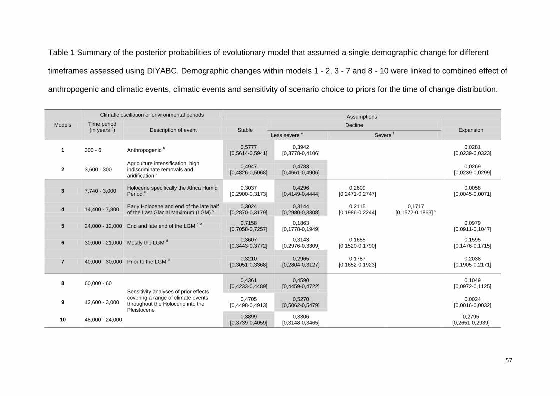
57
Table 1 Summary of the posterior probabilities of evolutionary model that assumed a single demographic change for different
timeframes assessed using DIYABC. Demographic changes within models 1 - 2, 3 - 7 and 8 - 10 were linked to combined effect of
anthropogenic and climatic events, climatic events and sensitivity of scenario choice to priors for the time of change distribution.
Models
Climatic oscillation or environmental periods Assumptions
Time period (in years
a)
Description of event Stable
Decline Expansion
Less severe e Severe
f
1 300 - 6 Anthropogenic b
0,5777 [0,5614-0,5941]
0,3942 [0,3778-0,4106]
0,0281 [0,0239-0,0323]
2 3,600 - 300 Agriculture intensification, high indiscriminate removals and aridification
c
0,4947 [0,4826-0,5068]
0,4783 [0,4661-0,4906]
0,0269 [0,0239-0,0299]
3 7,740 - 3,000 Holocene specifically the Africa Humid Period
c
0,3037 [0,2900-0,3173]
0,4296 [0,4149-0,4444]
0,2609 [0,2471-0,2747]
0,0058 [0,0045-0,0071]
4 14,400 - 7,800 Early Holocene and end of the late half of the Last Glacial Maximum (LGM)
c
0,3024 [0,2870-0,3179]
0,3144 [0,2980-0,3308]
0,2115 [0,1986-0,2244]
0,1717 [0,1572-0,1863]
g
5 24,000 - 12,000 End and late end of the LGM c, d
0,7158
[0,7058-0,7257] 0,1863
[0,1778-0,1949] 0,0979
[0,0911-0,1047]
6 30,000 - 21,000 Mostly the LGM d
0,3607 [0,3443-0,3772]
0,3143 [0,2976-0,3309]
0,1655 [0,1520-0,1790]
0,1595 [0,1476-0,1715]
7 40,000 - 30,000 Prior to the LGM d
0,3210 [0,3051-0,3368]
0,2965 [0,2804-0,3127]
0,1787 [0,1652-0,1923]
0,2038 [0,1905-0,2171]
8 60,000 - 60
Sensitivity analyses of prior effects covering a range of climate events throughout the Holocene into the Pleistocene
0,4361 [0,4233-0,4489]
0,4590 [0,4459-0,4722]
0,1049 [0,0972-0,1125]
9 12,600 - 3,000 0,4705
[0,4498-0,4913] 0,5270
[0,5062-0,5479] 0,0024
[0,0016-0,0032]
10 48,000 - 24,000 0,3899
[0,3739-0,4059] 0,3306
[0,3148-0,3465] 0,2795
[0,2651-0,2939]
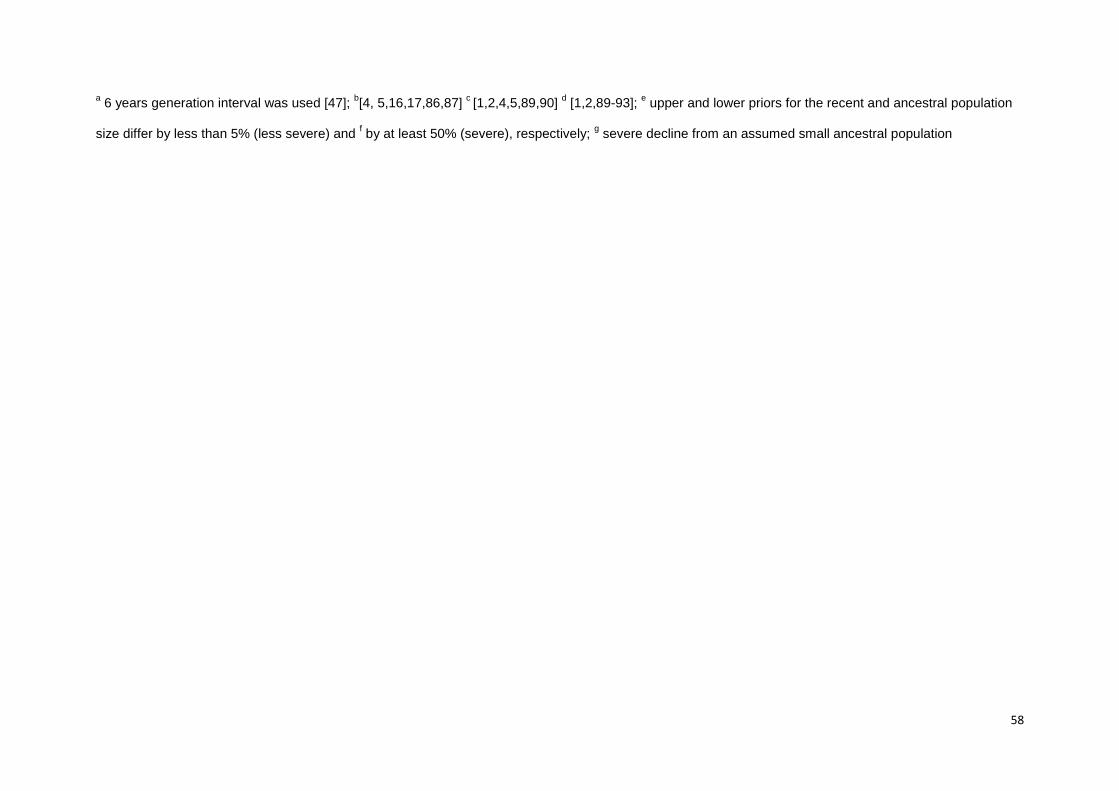
58
a 6 years generation interval was used [47];
b[4, 5,16,17,86,87]
c [1,2,4,5,89,90]
d [1,2,89-93];
e upper and lower priors for the recent and ancestral population
size differ by less than 5% (less severe) and f by at least 50% (severe), respectively;
g severe decline from an assumed small ancestral population
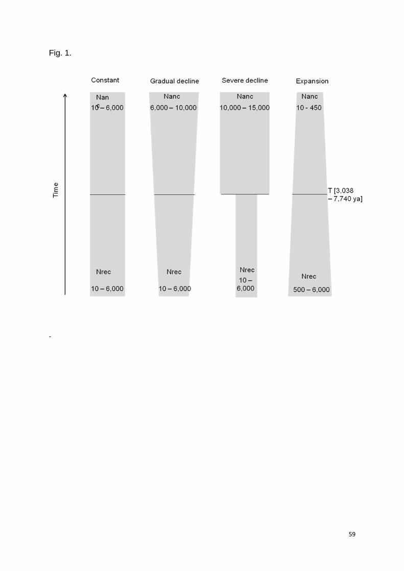
59
Fig. 1.
-
60
Supplementary information 1
Description and preliminary results using MSVAR1.3
MSVAR assumes that a stable population (N1) started to change in size, evolving
towards its current size (N0) linearly or exponentially, ta generations ago (T). The
model assumes mutations to follow a Stepwise Mutational Model (SMM) [1]. The
program employs a Markov chains Monte Carlo (MCMC) approach to generate
posterior probability distributions for N0, N1 and T, based on the full allelic distribution
contained in the data combined with these parameters’ prior (log normal) and
hyperprior distributions.
We performed six independent runs of 2 X10⁹ iterations, with thinning values
of 100,000, and two others of 4 X 10⁹ iterations thinned every 200,000 steps, in both
cases with 20,000 samples recorded (Table S7). The two longer chains contrasted
scenarios assuming stable populations, but differed as one assumed an exponential
and the other a linear population growth mode. The remaining four runs assumed an
exponential growth mode. The exponential mode was favoured as it is considered
more realistic when assessing the impact of more recent events, such as
anthropogenic factors [1]. Chains also differed in the mean hyperprior for the
mutation rate, which for long chains was set to 10-3 versus 10-6 for the shorter chains
based on preliminary runs (Table S7). We set N0 = N1 or N0 > N1 (i.e. assessed for
stability or expansion, respectively) at different time spans in order to consider
scenarios that are alternatives to the classically proposed bottleneck [2,3]. We used
different sampling strategies by setting vague priors for N1 and T, and "uninformative
priors" for N0. The use of broad priors was applied to reduce their influence on
posterior distributions. The broad parameter space for T encompassed both recent
61
(< 1000 ya) and ancestral (> 1000 ya) timeframes (Table S7). Thus, we attributed
any demographic change occurring more than 1000 ya as linked to climatic
oscillations, while more recent (1000 ya to the present) due to a combination of
anthropogenic and climatic factors. In order to convert time of change into years (T)
and due to uncertainty in the cheetah’s mean generation time, we considered
estimates of 2.4 years [4,5], 4.05 years (Fabiano et al. unpublished data [see chapter
3]) and 6 years [6]. The first value is based on long-term monitoring data for females,
and the third on data from zoological institutions; the 4.05 estimate derives from
VORTEX simulations that incorporate life history parameters.
To check for convergence, we discarded at least the first 50% of the recorded
values and applied the Geweke, and Gelman and Rubin diagnostic tests to the
individual and combined data sets, respectively, as implemented in the CODA R
package [7]. A value of 1.1 - 1.2 for the corrected scale reduction factor served as an
indicator of distribution stabilization [1]. CODA was also used to compute the model
parameters’ marginal posterior distributions, point estimates (mean, median and
mode) and 95% highest probability densities (HPD). In order to assess the relative
probability of alternative scenarios, i.e. whether demographic changes are recent
(T0) or ancestral (T1), Bayes factors (BF) were computed. This involved counting the
number of times the ratio between the posterior distributions of two scenarios were
lower, equal or greater than one. For instance, a BF of one (i.e. (T0 / T1 > 1) / (T0 /
T1 < 1) = 1) is indicative that both scenarios are equally probable, whereas BF > 1 or
< 1 indicate that a more recent or ancestral time of change was favoured,
respectively (after [8]). BF values between four and seven and > 7 served as
indicators of positive and significant evidence for a scenario, respectively. These
comparisons of BF across different time intervals also allowed the assessment of
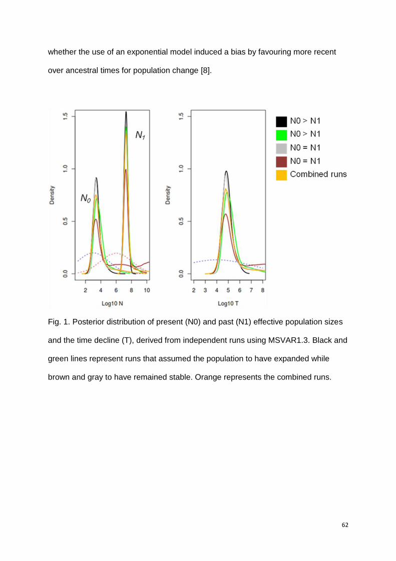
62
whether the use of an exponential model induced a bias by favouring more recent
over ancestral times for population change [8].
Fig. 1. Posterior distribution of present (N0) and past (N1) effective population sizes
and the time decline (T), derived from independent runs using MSVAR1.3. Black and
green lines represent runs that assumed the population to have expanded while
brown and gray to have remained stable. Orange represents the combined runs.
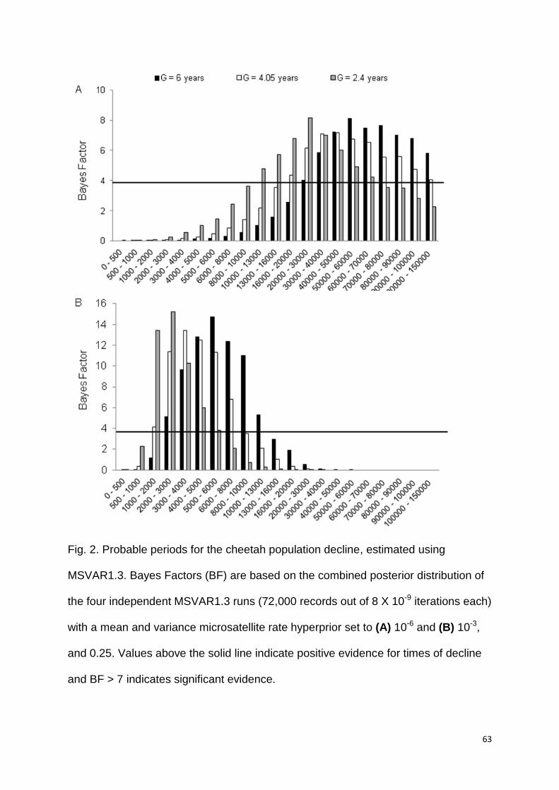
63
Fig. 2. Probable periods for the cheetah population decline, estimated using
MSVAR1.3. Bayes Factors (BF) are based on the combined posterior distribution of
the four independent MSVAR1.3 runs (72,000 records out of 8 X 10⁻⁹ iterations each)
with a mean and variance microsatellite rate hyperprior set to (A) 10-6 and (B) 10-3,
and 0.25. Values above the solid line indicate positive evidence for times of decline
and BF > 7 indicates significant evidence.
64
References
1. Beaumont MA (1999) Detecting Population Expansion and Decline Using
Microsatellites. Genetics 153: 2013 – 2029.
2. O’Brien SJ, Roelke ME, Marker LL, Newman A, Winkler CA, et al. (1985) Genetic
basis for species vulnerability in the cheetah. Science 227: 1428 – 1434.
3. O’Brien SJ, Wildt DE, Bush M, Caro TM, FitzGibbon C, et al. (1987) East African
cheetahs: evidence for two population bottlenecks? PNAS 84: 508–511.
4. Kelly, MJ (2001). Lineage Loss in Serengeti Cheetahs: Consequences of High
Reproductive Variance and Heritability of Fitness on Effective Population Size.
Conserv. Biol. 15, 137–147.
5. Bisset C, Bernard RTF (2011) Demography of Cheetahs in Fenced Reserves in
South Africa: Implications for Conservation. S Afr J Wildl Res 41: 181–191.
6. Marker L, O’Brien SJ (1989) Captive breeding of the cheetah Acinonyx jubatus in
North Amercian Zoos (1871 - 1986). Zoo Biology 8: 3 – 16.
7. Plummer AM, Best N, Cowles K, Vines K, Plummer MM (2011) Package “ coda ”:
1 – 44.
8. Quéméré E, Amelot X, Pierson J, Crouau-roy B, Chikhi L (2012) Genetic data
suggest a natural prehuman origin of open habitats in northern Madagascar and
question the deforestation narrative in this region. PNAS: 1–6.
doi:10.1073/pnas.1200153109.
65
Supporting information 2
Table 1. Estimates of cheetah subspecies divergence times.
Table 2. Prior distributions for models assessed using DIYABC. Models 1 - 10
assessed whether the population had declined, been stable or expanded during
different timeframes. In addition, categories 3, 4, 6 and 7 included a scenario of
severe decline (upper and lower prior of the recent and ancestral population size
differed by at least 50% versus 5%). Categories 8 - 10 assessed the impact of
broader prior distributions on model selection.
Table 3. Prior distributions for sensitivity analyses that assessed the impact of a
broader prior distribution of the geometric mean governing allele size variation on
model selection using DIYABC.
Table 4. Confidence in scenario choices based on type I and type II errors, and
statistical power (1 - type II error) for the two scenarios with the highest relative
posterior probability of simple scenarios assessed using DIYABC. Type I error was
computed as the number of times a "true" scenarios did not have the highest
posterior probability (HPP) and II, as the number of times it had the HPP when the
data were simulated under a different scenario.
Table 5. Assessment of model fit based on the summary statistics (Ss) ability to
recover similar genetic diversity as that observed in the observed data, in the case of
simple scenarios assessed using DIYABC. Ss ≤ 0.5 were significant (Moyer et al.
2009). NAL = mean number of alleles and MGW = mean ratio of the number of
alleles over the range of allele sizes.
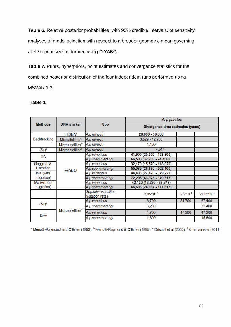
66
Table 6. Relative posterior probabilities, with 95% credible intervals, of sensitivity
analyses of model selection with respect to a broader geometric mean governing
allele repeat size performed using DIYABC.
Table 7. Priors, hyperpriors, point estimates and convergence statistics for the
combined posterior distribution of the four independent runs performed using
MSVAR 1.3.
Table 1
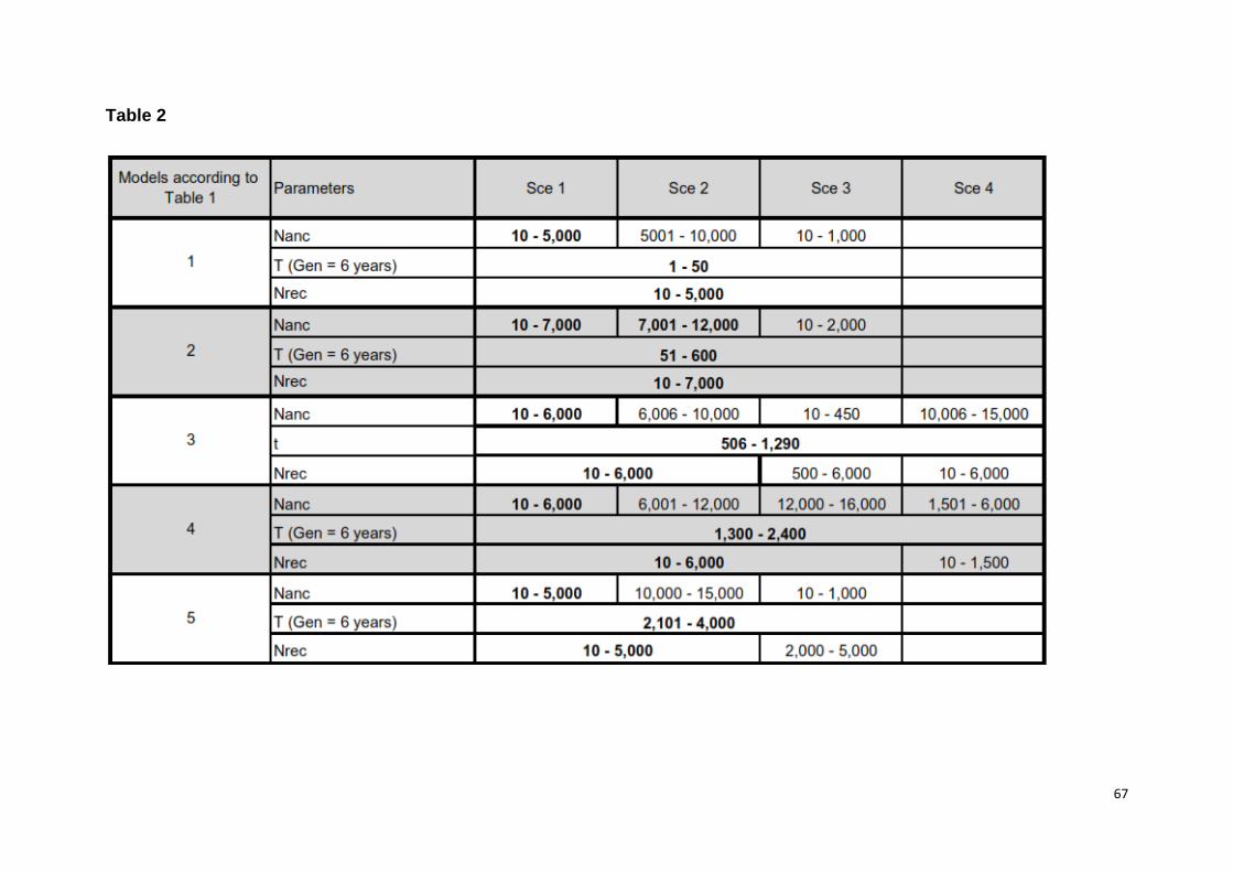
67
Table 2
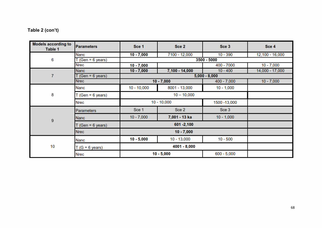
68
Table 2 (con’t)
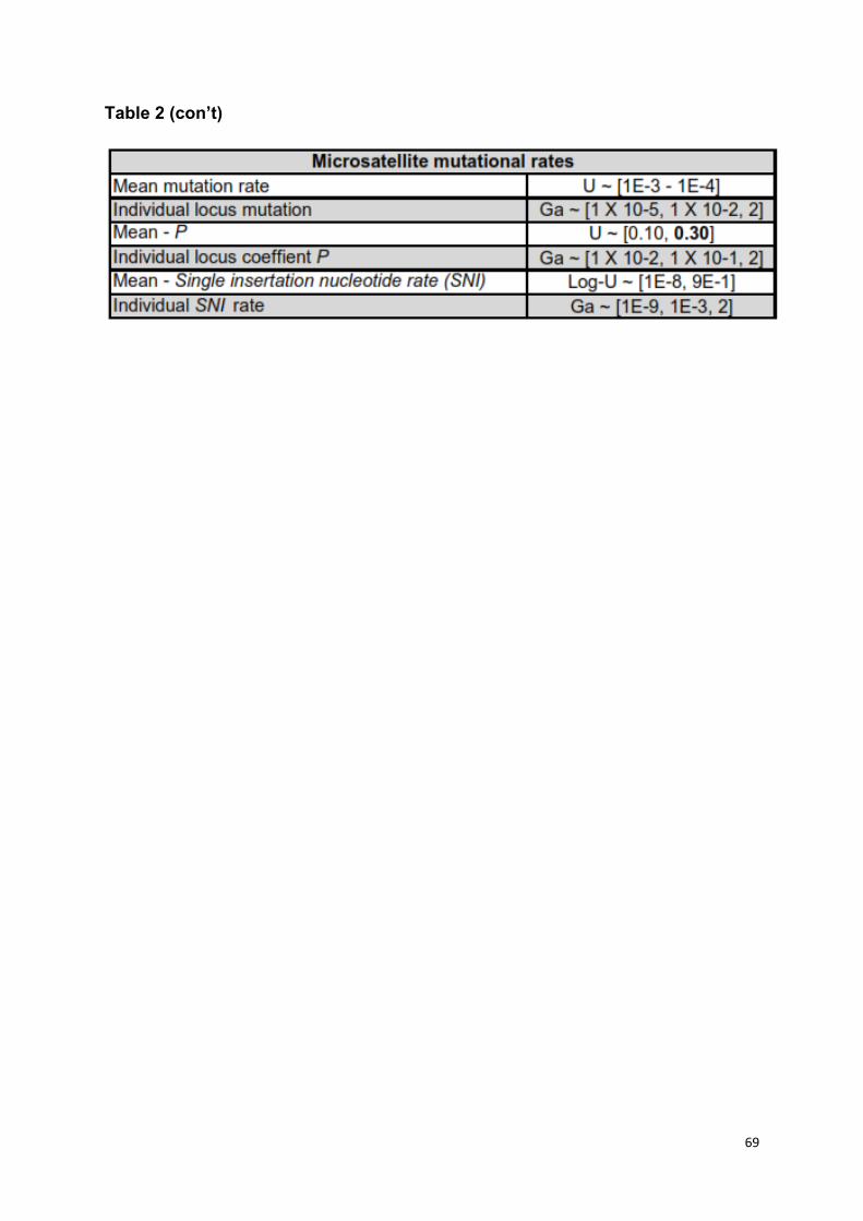
69
Table 2 (con’t)
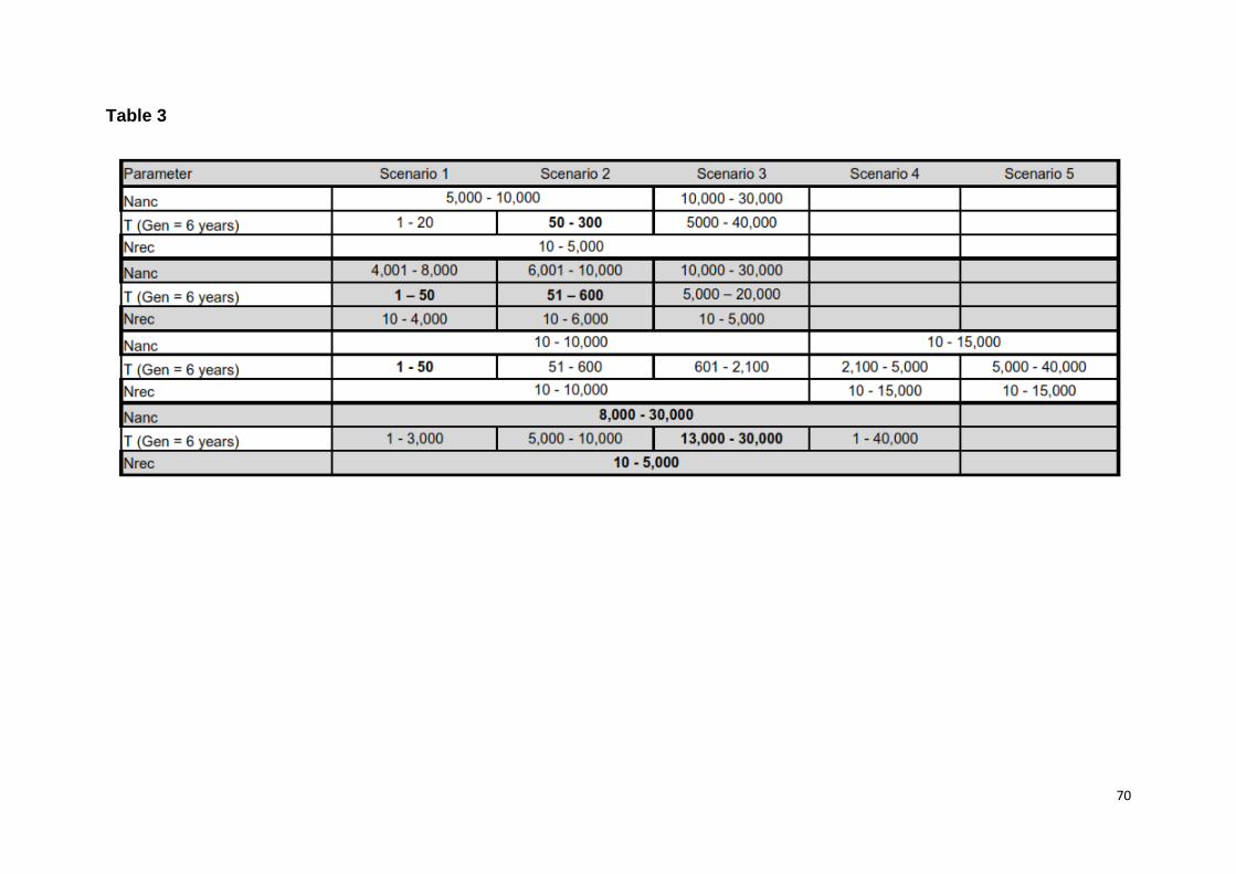
70
Table 3
71
Table 3 (con’t)
72
Table 4
73
Table 4 (con’t)
74
Table 4 (con’t)
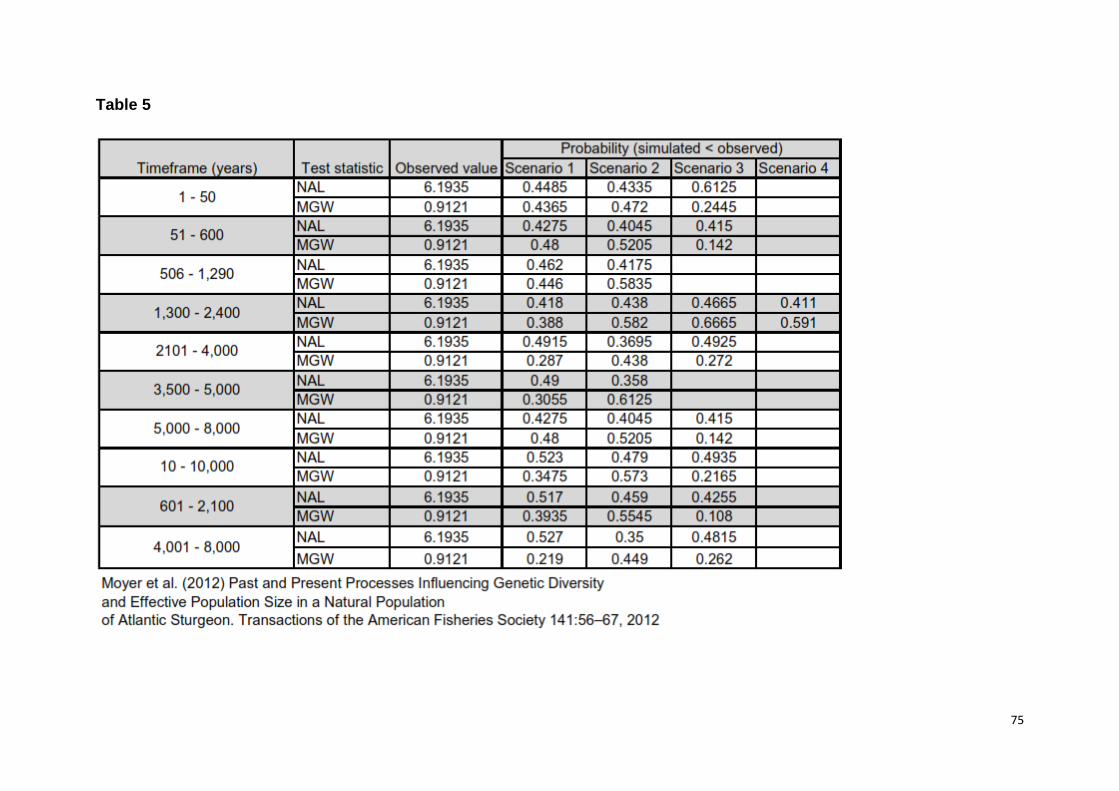
75
Table 5
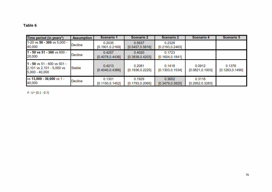
76
Table 6
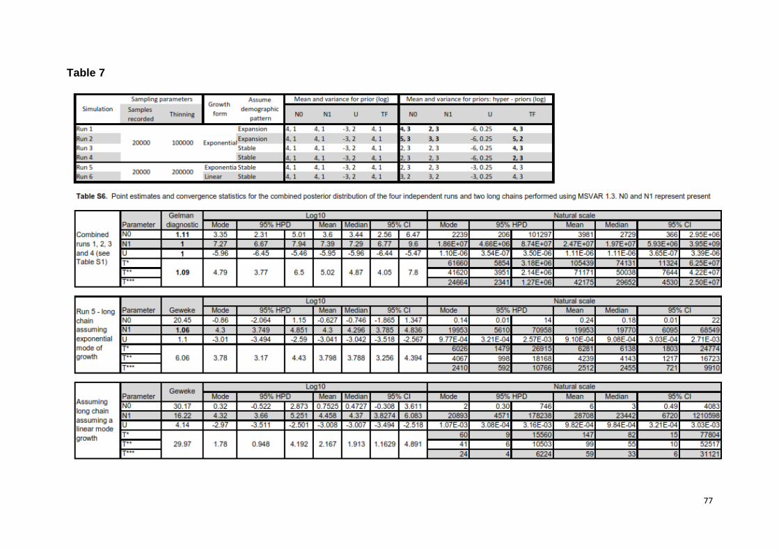
77
Table 7

78
CHAPTER III
79
Estimating the effective population size of the Namibian cheetah Acinonyx
jubatus: comparison of analytical approaches and assessment of the impact of
vital rate variation.
Author list:
Ezequiel Chimbioputo Fabiano a,b,c
Laurie Marker b
Anne Schmidt-Küntzel b, c
Eduardo Eizirik a
Affiliations:
a. Laboratório de Biologia Genômica e Molecular, Faculdade de Biociências,
Pontifícia Universidade Católica do Rio Grande do Sul, Porto Alegre, RS 90619-900,
Brazil
b. Cheetah Conservation Fund, PO Box 1755, Otjiwarongo, Namibia.
c. Life Technologies Conservation Genetics Laboratory, Cheetah Conservation
Fund, PO Box 1755, Otjiwarongo, Namibia.
Email addresses:
80
Corresponding authors:
Ezequiel C. Fabiano, Cheetah Conservation Fund, PO Box 1755, Otjiwarongo,
Namibia. Email: [email protected], [email protected]
Prof. Eduardo Eizirik, Laboratório de Biologia Genômica e Molecular, Faculdade de
Biociências, Pontifícia Universidade Católica do Rio Grande do Sul, Porto Alegre,
RS 90619-900, Brazil, Email: [email protected]
Structure details:
Text pages: 17
Number of Figures: 2
Number of Tables: 2
81
Abstract
Ne is necessary to assess the genetic viability of large conservation species. The
long-term viability of a population is often associated with an effective population size
(Ne) threshold value of > 500. Ne is expected to be smaller than the total population
size (Nc) and may be influenced by independent factors. We used two one-sample
genetic and one demographic estimator to determine the contemporary Ne of the
Namibian cheetah population. We also assessed the sensitivity of Ne to
perturbations in survival rates, proportion of breeders as well as uncertainties in
carrying capacity and Nc. Genetic estimates (134, 95% CI 99 - 224) were
significantly less than 500 and demographic estimates, which ranged from 450 to
2500 depending on generation time used (2.4 or 6 years). Demographic Ne
estimates were mostly sensitive to perturbations in the proportion of females
breeding, adult female survival rates, uncertainties in Nc and the carrying capacity.
These same parameters also influenced Nc. We observed contrasting effects due to
different perturbations levels of the same parameter, possibly due to non-linear
responses by factors affecting Ne and Nc. Overall, our finding suggests that the
population is viable but Ne changes according to the contemporary status of
demographic parameters. Conservation actions should continue to focus on aspects
related to females.
Keywords Population viability • Reproductive variance • Linkage disequilibrium •
Survivorship patterns • Simulation modeling
82
1. Introduction
Population viability is governed by interactions among several demographic
parameters, in particular its census (Nc) and effective (Ne) sizes. As a result,
conservation actions often aim to maximize both measures. These two measures
differ in that Nc represents the total annual population size, while Ne the size of an
ideal Wright-Fisher (WF) population that presents the same genetic properties (e.g.
drift-induced rate of loss of genetic diversity) as the study population (Palstra and
Fraser 2012). An ideal population is characterized by random mating, discrete
generations, reproduction success following a Poisson distribution, and even sex
ratio, in addition to being closed, having drift as the only source of linkage
disequilibrium, and being assessed only for unlinked loci) (Charlesworth 2009). The
Ne/Nc ratio varies across species (Nunney 1993; Frankham 1995; Palstra and
Ruzzante 2008) and among subpopulations (Phillipsen et al. 2011) . Ne is highly
susceptible to fluctuations in Nc, among other variables (Frankham 1995; Vucetich
and Waite 1998) importantly, populations with large Nc can have low Ne, and hence
experience substantial genetic drift (Hedrick 2005; Hare et al. 2011). Consequently,
in the context of conservation planning there is a need to determine a population’s
contemporary Ne, and to assess its sensitivity to varying threat and management
scenarios (Andrello et al. 2012; Baalsrud 2011).
The cheetah, Acinonyx jubatus, is classified as Vulnerable by IUCN with less
than 12,000 living individuals spread across 22 countries (Durant et al. 2008).
Currently, only Namibia and Botswana possess adult population sizes above 1000
individuals, with at least 2,000 and 1,800 individuals, respectively (Purchase et al.
2007). Common threats of extinction across the range of this species include habitat
loss, fragmentation and degradation, as well as human-wildlife conflict (HWC)
83
(Sunquist and Sunquist 2002; Purchase et al. 2007; Durant et al. 2008). Moreover,
HWC has been deemed the determining factor of Namibia’s current and future
ecological carrying capacity (Turpie et al. 2010). Population viability analyses, as
measured by a positive growth rate (λ >1), indicate that the cheetahs are vulnerable
to total mortality rate patterns (natural and additive) and reproduction patterns (Berry
et al. 1997; Crooks et al. 1998; Kelly and Durant, 2000; Lubben et al. 2008).
Consequently, conservation strategies have so far focused on increasing survival
rates and limiting the removal of females. However, it remains unknown how these
actions and removal of different age classesaffect Ne.
The Namibian cheetah population has fluctuated and declined during the past
century due to diverse factors including droughts, prey reduction, trophy hunting and
indiscriminate removals resulting from human wildlife conflict (HWC) (O’Brien et al.
1987; Nowell 1996; Marker-Kraus et al. 1996; Marker et al. 2007). These fluctuations
and removals certainly have caused Nc to fluctuate, induced differences in survival
rate patterns and an unstable age structure, reduced the actual and potential number
of breeders (Marker et al. 2003), as well as altered generation times (G).
Furthermore, these processes likely caused increases in family size variances
(Saether, Engen and Solberg 2009). All these factors affect Ne in concert or
independently, as they are violations of some of the WF model assumptions (Nunney
and Elam 1994; Waite and Parker 1996). This is an important issue, as Ne estimates
are biased if estimators do not account for these violations (Jorde and Ryman 1995,
2007). Therefore, as the degree of robustness of Ne estimators to violation of WF
assumptions differ (Luikart et al. 2010) studies assessing Ne should apply multiple
estimators.
84
In this study, we computed inbreeding Ne estimates for the Namibian cheetah
population, and assessed their variability as a function of uncertainty in the initial
population size (Ninit), carrying capacity (K), and vital rates (mortality and
reproduction). We also estimated the impact of these variables on the estimates of
Nc, deterministic λ, sex ratio (SR) and G. To estimate Ne, we applied two different
‘one-sample’ genetic estimators, one based on linkage disequilibrium (LD) (Hill 1981)
and implemented in the program LDNe (Waples 2006; Waples and Do 2008), and
the other using Approximate Bayesian computation (ABC) and implemented in the
software ONeSAMP (Tallmon et al. 2008). A demographic estimator, based on a
strategy that uses heterozygosity levels derived from simulations of population
processes, was also computed (Eizirik et al. 2002; Sato and Harada 2008). Genetic
and demographic estimators are complementary, as they may reflect different
historical time frames and be affected differently by various population processes
(Nunney and Elam 1994; Wang 2012, et al. 2010, 2012; Waples and Waples 2011).
Ultimately, the study aim was to allow an improved understanding of the processes
affecting cheetah population dynamics, and their impact on long-term genetic
viability in this population.
2. Methods
2.1. Dataset construction and genetic estimates of Ne
To estimate Ne using genetic approaches, we used a set of 90 unrelated cheetah
individuals captured by farmers between 1991 and 1999, and previously genotyped
for 36 dinucleotide microsatellite repeats (Marker et al. 2008). From this initial panel,
however, only 31 loci were used due to the data requirements of some estimators
(e.g. ONeSAMP requires that only polymorphic loci with limited missing data are
used (Tallmon et al. 2008)).
85
We obtained Ne estimates using LD, with the approach implemented in LDNe
(Waples, 2006; Waples and Do, 2008), and also through the ABC method available
in ONeSAMP (Tallmon et al. 2008). LDNe employs the Burrow Δ measure of LD for
estimating Ne (Waples and Do 2008). Ne was computed assuming random mating,
and using the jacknife model to compute 95% confidence intervals (CI). Preliminary
results using the recommended Pcrit = 0.02 for n > 25 (Waples and Do 2010) yielded
similar results (95% CI overlap) as Pcrit = 0.01 and 0.05, here we report the average
of these three estimates.
The ONeSAMP estimate, in contrast, uses seven summary statistics (SS) that
are a function of Ne and a prior range supplied for Ne when computing the posterior
estimate of this variable (Tallmon et al. 2008). We performed three runs, using 20
with 1500 or 2000 as priors. Ne estimates are inferred through a weighted local
regression based on a subset of the 50,000 posterior records that have the most
similar SS to those of the observed data set. Despite some variability in Ne estimates
based on different priors, these overlapped (e.g., Phillipsen et al. 2011), thus we
report the harmonic mean of Ne estimates across runs. Following Waples and Do
(2010), LDNe and ONeSAMP estimates were combined in an attempt to increase
overall Ne precision.
2.3. Demographic-based Ne estimation
2.3.1. Ne and Ne/Nc estimation
Demographic Ne estimates were determined using a hybrid strategy based on
population simulations. We used the Population Viability Analysis (PVA) software
VORTEX (Miller and Lacy 2005) to simulate demographic processes, and then used
a genetic approach to calculate Ne based on the observed loss of heterozygosity
86
along the simulations. VORTEX model structure is presented in S1. We used the
formula Ne = ½(1- exp (logeHt)/t) (Crow and Kimura 1970; after Rieman and Allendorf
2001; Eizirik et al. 2002), where Ht is VORTEX's estimate of heterozygosity and t the
number of years (yrs) in a simulation divided by the G. Due to uncertainties in G
estimates, Ne was computed using G of 2.4, 5.34 yrs (Kelly 2001), 6 yrs (Marker and
O’Brien 1989;) and 4.05 yrs (this study). Ne based on these G estimates are referred
accordingly to as Ne5, Ne4, Ne3 and Ne1. To calculate Ne/Nc ratios, we used VORTEX's
Nc estimate after the simulations. Overall, 45 different scenarios were simulated
including the baseline scenario, and each scenario was replicated three times; we
therefore report averages for Ne and Nc across replicates for each scenario.
2.3.2. Baseline scenario input parameters
Input parameters were drawn from the literature (Marker et al. 2003, 2008; Lindsey
et al. 2009) and are summarized on Table 1. The scenario based on these values
was treated as the baseline scenario, representing a hybrid between the population
realistic and biological potential. Appendix S1 presents a detailed rationale for their
inclusion, as well as parameter estimation approaches. Below we provide a brief
overview, specifically focusing on parameters that were recalculated. Overall, we ran
45 models, each of them comprising 500 iterations spanning 200 yrs and defining
extinction as when only one sex remained. The population was assumed to be
panmictic (Marker et al. 2008). Ninit and K were set to 3670 individuals, according to
a crude extrapolation of a minimal density of 5.3 individuals (inds.) per 1000 km2
(Fabiano et al. in revision, Chapter IV) to an area of 692,404 km2 (after Hanssen and
Stander 2004). This estimate is conservative, as Ninit could be > 11,000 inds., if we
considered a higher density estimate of 16 inds. / 1000 km2 (Fabiano et al. in
revision, Chapter IV). The proportion of males in the breeding pool was set to 62%, a
87
value estimated by dividing total number of adult males (≥ 3 years) by the total
number of males captured by farmers from 1991 to 2011. In addition to only counting
the adults, only one male per coalition was counted. This proportion may be
overestimated due to sampling bias and if the population is characterized by a
polygynous-polyandry mating system as observed for cheetahs in the Serengeti
(Gotelli et al. 2007). Harvesting rates were set as the maximum number of
individuals handled by the Cheetah Conservation Fund (CCF) per age class between
1991 and 2011 recorded. Mortality rate (qx) estimates were determined using BaSTA
(Bayesian survival trajectory analysis) (Colchero et al. 2012; Colchero and Clark
2012) based on a data set of 90 aged dead cheetahs handled by CCF between 1991
and 2011. The data set included 64 males and 26 females ranging from cubs to 12-
year-old animals. Mortality estimates reflect total mortality, including natural and
anthropogenic. For the qx SD, we followed Stacey and Taper (1992) (S1).
2.3.2.1 Sensitivity analyses of viability, and relationship among population
parameters
Sensitivity analyses were performed by decreasing baseline mortality rates and the
proportion of breeders by 10% (low), 20% (moderate) and ≥ 40% (high), while other
parameters were kept constant (S2). For example, to assess the impact of survival
rates of active breeding females we increased simultaneously the survival rates for
adult female and cubs (age 0 - 1) by 10, 20 or 40% (e.g. F2M0-1F0-1 (10%) in Fig.
1, Table S2). It is northworthy that while some scenarios are of direct relevance to
conservation others provide a through understanding of processes affecting Ne (e.g.
survival rate of cubs, M0-1). To investigate the effects of these varying vital rates on
Ne, Nc, λ, SR and G, we determined the percentage change in each of these, relative
to the baseline estimate of each parameter. The significance of parameter response
88
to perturbation levels was determined through the Kruskal-Wallis test (KW). In
addition, we used an analysis of variance (ANOVA) to ascertain whether Ne
estimates differed among the assumed values of G. Pearson's correlation coefficient
(r) was used to determine the significance of the relationship among Ne estimates,
and Spearman’s rho to assess it among Ne, Nc, λ, SR and G. Since preliminary
results indicated that Ne based on G = 6 (Ne3), 5.34 (Ne4) and 2.05 yrs (Ne5) only
differed in their magnitude, we focus mostly on Ne3 and Ne5.
3. Results
3.1. Genetic-based Ne estimates
LDNe yielded a Ne estimate of 119 individuals (95% CI 94 - 156), while that
calculated with ONeSAMP was 153 (95% CI 99 - 392), with a combined Ne estimate
of 134 (95% CI 99 – 224, coverage 0.933). Despite differences in precision,
estimates were not significantly different (t = 2.55, d.f. = 4, p > 0.05). A noteworthy
observation is that they were all significantly lower than 500 (one sample t = - 27.05,
d.f. = 5, p < 0.01), which often used as a threshold value for determining long-term
genetic viability (Allendorf and Luikart 2007). When the combined Ne estimate is
multiplied by a six years generation time we obtained an approximate generational
Ne of 804 (95% CI 594 – 1344). Using VORTEX Ninit of 3670, we obtain a Ne/Nc ratio
of 0.16 (CI 0.22 - 0.37).
3.2 Demographic-based Ne estimates
Final heterozygosity estimates for all 45 scenarios ranged from 0.9601 to 0.9806
(baseline [b] of 0.9701) and resulted in Ne estimates of approximately 450 to 2500
(Neb of 550 - 1650), conditioned on G (Table S1). These estimates were significantly
89
higher than genetic-based estimates (ANOVA F = 809.57, p < 0.01). Furthermore, Ne
estimates based on different G values differed significantly amongst themselves
(ANOVA F = 529.37, p < 0.01), with smaller G associated with larger Ne estimates
(Table S1). This highlights the importance of considering multiple G estimates when
estimating Ne even for the same population. Nevertheless, these were highly
correlated (r = 95%, p < 0.01; Table 2).
3.2.1 Sensitivity of viability analysis to perturbations in vital rates and uncertainties in
population parameters
The sensitivity of Hexp, Ne, Nc, λ, SR and G to perturbations in survival rates,
proportion of breeders, Ninit and K indicate their susceptibility to various sources of
uncertainties and or conservation actions. In general, most perturbations resulted in
Hexp, Ne and Nc estimates higher by 50% relative to baseline values, except for λ
(34%) and G (14%) (Table 2, Fig. 1).
Hexp was on average 0.9722 ± 0.0039 with a 40% and 10% decline in the
proportion of breeding females determining its range (0.9601 – 0.9805). It decreased
with a 40% and 20% reduction in the proportion of males breeding and Ninit,
respectively. Hexp increased with declines of at least 40% in K and with a
simultaneous decline of 20% in adult female mortality and non-adults (irrespective of
gender) (Fig. 1a). In turn, Ne increased in direct proportion to increases on adult
survival, particularly that of females (Fig. 1b, c, d; Table S2). For instance, increases
of 10%, 20% and 40% in adult female survival resulted in an increase of 8%, 14%
and 22% in Ne, respectively, versus increases of only two, three and six percent due
to increases on male survival. Ne was also increased with shorter G (i.e. 1810 ± 268
90
inds, G = 2.4 yrs; 876 ± 112 inds, G = 4.05 yrs; 680 ± 100 inds, G = 6 yrs) (Table
S2).
Even though Hexp and Ne are directly linked differences in the magnitude of
perturbations of three scenarios resulted in contrasting effects (Fig. 1a. b, c, d). First,
a reduction in the proportion of breeding females of 10% yielded an increase of
1.07% and 54% on Hexpb and Neb respectively, while a reduction of 20% caused
these values to decrease by at least 0.42 and 14%, respectively. Second, a
reduction in K of 40% (K = 2202) increased Ne, while a decline of 20% (K = 2936)
deflated Ne. Third, a 20% decrease in Ninit (Ninit =2936) increased Hexpb and Neb by
0.83% or 19%, respectively, while a decrease of 40% (Ninit = 2202) caused Hexpb and
Neb to decline by -0.9% and -3%, respectively. Overall, Hexp and Ne were most
sensitive to perturbations on the proportion of breeders, followed by uncertainties in
Ninit, and or K and moderate concurrent increases of adult female survival and that of
non-adults.
Nc values ranged from 10 to 3550 individuals (Ncb = 790) and it was positively
influenced by 10% decreases on the Ninit, the proportion of female reproducing and
the survival rates for all female age classes and that of adult males (Fig. 1e, Table
S2). The latter, had a lesser impact than declines on female (Table S2). On the
contrary, Nc declined with at least a 20% reduction in the proportion of female
breeders and K and with a 40% ≤ reduction in Ninit, similar to Hexp and Ne.
Furthermore, increases of 10% to 40% in non-adult male mortality also affected Nc
negatively (Fig. 1e).
A severe skewed adult female SR was prevalent in all but two scenarios (0.38
± 0.06, excluding an outlier of 0.99) (Fig. S1g). Only moderate and or high declines
91
in male cubs and adults, respectively caused SR to ~ 1:1 (male: female). Likewise,
declines of 20% in the proportion of females breeding or 80% in adult female survival
also reduced SR to 0.6:1. Otherwise, perturbations in female survival only
accentuated this bias whereas those involving male survival had the opposite effect.
The population was self-sustaining λb = 1.10 (1.12 ± 0.06, range 0.97 - 1.28)
with λ positively influenced by increases in adult female survival rates, concurrently
or not with that of non-adults. On the other hand, λ declined with decreases in the
proportion of breeding females while 26 scenarios mostly those involving increases
on male survival rates, declines on Ninit or K had no influence on λ (i.e. λb = 1.10).
G was on average 4.16 ± 0.23 years (Gb = 4.05, range 3.98 - 5.15 yrs) (Fig.
1i). Increases in females' survival rates reduced Gb by -2 to -0.2% but it increased
with moderate and high declines in adult mortality by 0.4% to 27.3%. Furthermore,
Gb increased with a concurrent moderate decreases in female and male cub (~ 6%)
(Fig. 1i). G was unaffected by increases in non-adult males, and declines in the
proportion of males breeding, Ninit, K and moderate declines in combined adult
survival.
Ne/Nc ratio among all Ne's ranged from 0.21 and 3.75, with 64%, 93% and
27% of Ne1 and Ne3 (n = 44), and N5/Nc (n = 43) < 1, respectively (Fig. 2, Table S2).
Range bounds were primarily the result of a 20% reduction on the proportion of
females breeding and a high (80%) decline of adult male mortality. By excluding
these we observed narrower ranges (Ne1, Ne3 and N5/Nc of 0.27 - 1.21, 0.21 - 0.82
and 0.64 - 2.45, respectively). In addition, to Ne/Nc ratios varying with G used to
determine Ne with Ne5 (G = 2.4 yrs)/Nc > Ne1 (4.05 yrs)/Nc or Ne3 (6 yrs)/Nc, these also
vary based on gender-specific survival rates. Scenarios involving reductions in

92
female survival simultaneously or not with that of cubs were predominantly less than
0.5 while above 0.5 for those involving male survival rates (Fig. 2). It is noted that
Ne/Nadults had comparable pattern as Ne/Nc (ranged from 0.40 to 7.12 with Ne1, Ne3
and N5/Nadults being ≥ 1 by 70%, 55% and 100%, respectively).
3.2.2 Relationship among Ne, Nc, λ, SR and G
Ne’s correlated positively and significantly with Hexp, Nc, Nadult, G, λ but not with SR
(Table 2). Furthermore, correlations between Hexp and Nc, Nadult or G, G and λ, λ and
Nc, were also significant (Table 2). A correlation between SR and λ was negative but
significant. In general, even though high Ne estimates were associated with high Nc
this was not always when G, SR and λ were their highest (Fig. 2).
4. Discussion
The study findings indicate that the population is likely to be genetically and
demographically viable, even though one-sample genetic estimates were below the
recommended viability threshold value of 500 (Allendorf and Luikart 2007).
Sensitivity analyses indicate that this viability is susceptible to moderate declines in
the survival of single adult females or those accompanied by cubs, as well as low
declines in the proportion of females breeding. In addition, moderate or high levels in
uncertainty in population size (Ninit) or carrying capacity (K) influence the viability
estimate in itself. These factors also influenced the census size (Nc), growth rate (λ)
and mean generation time (G), but the magnitude and direction of influence differed
among these variables. Hence, even though the influence of certain conservation
actions on Ne and Nc or Nadult may be positive, others may have an opposite effect,
causing Ne/Nc ratio to fluctuate. Nevertheless, in order to maximize the evolutionary
93
potential of this population, conservation actions should concentrate on aspects
primarily related to females.
Below, we argue that the population is likely viable, even though genetic Ne
estimates were significantly below the often recommended threshold value. Second,
that underlying processes and nonlinear response of demographic parameters,
along with their interaction with life history traits, variance in family size and
longevity, explains the sensitivity of viability estimates to perturbations.
4.1 Genetic and demographic Ne estimates
The observed genetic estimates were significantly lower than demographic ones and
than 500, a result that might indicate that the population is not viable in the long
term, due to limited evolutionary potential. However, due to the violations of some of
the genetic estimators’ underlying assumptions, these Ne estimates may be
downward biased. First, the discrete generation assumption was violated, as
cheetahs have overlapping generations. LDNe is susceptible to this violation
(Waples and Do 2010) often introduces a negative bias (Palstra and Ruzzante 2008;
Waples 2010). The bias originates from differences in individual and cohort lifetime
reproductive success (Jorde and Ryman 1995; Engen et al. 2005; Engen et al. 2007;
Waples 2010) that are functions of age-specific survival and birth rates (Jorde and
Ryman 1995; Saether et al. 2009). In addition, because generational Ne is
conditioned on lifetime reproductive success, Ne estimates may represent the
parental cohort(s) of the sample or an intermediate value between this and Ne
(Waples 2005; Waples and Do 2010). In this study, the congruence of genetic
estimates with demographic estimates, after having been multiplied by generation
times, supports this relation. However, this conjecture requires further assessment
94
(Waples and Do 2010; Skrbinsek et al. 2011). Nevertheless, unless estimators
account for these sources of variance, Ne estimates will be biased.
A second possible cause of negative bias is the small sample sizes (S),
particularly relative to the number of cohorts in the dataset. As alluded, the latter
introduces LD which is accentuated if S is low, as only small fractions of the progeny
of different cohorts are likely to have been sampled (Luikart et al. 2010). Moreover,
this violates the assumption that genetic drift was the only cause of allelic variance in
the data set (Waples 2006; Tallmon et al. 2008). Furthermore, unequal sample sizes
across loci may increase sampling noise causing Ne to deflate as some of this noise
is treated as drift (Peel et al. 2013). Indeed, the LDNe 95% CI ranged from 624 to
infinity based on 88 inds and 36 loci (data not shown).
Lastly, LDNe is susceptible to fluctuations in Nc (Vucetich and Waite 1996;
Waples 2006; Luikart et al. 2010) and, given that the study population has been
neither stable nor closed over ecological timescales, these likely have influenced Ne.
The population has declined during the past century due to various reasons including
droughts, prey reduction, habitat loss and human wildlife conflict (HWC) (Marker-
Kraus et al. 1996; Nowell 1996; Marker et al. 2007). For instance, like selective
harvesting (Harris et al. 2002; Milner et al. 2007), HWC possibly affected Ne directly
(e.g. removals of adults, primarily males) or indirectly (e.g. removal of females
accompanied by cubs) (Marker et al. 2003). Sensitivity analysis results support this
conclusion, as Ne was reduced with a 40% decline in Ninit (2200 vs. 3670) and in the
proportion of breeding individuals (Fig. 1a). As LD can persist for a few generations
(Luikart et al. 2010; Waples 2006) Ne may reflect periods prior to the 1990's, when
Ne could have been lower due consistently high removal rates (Marker-Kraus et al.
1996; Nowell 1996). Noteworthy it is that, if we consider the suggestion that to obtain
95
accurate genetic estimates, at least 10% of the true Ne needs to be sampled so as to
maximize S/Ne (Palstra and Ruzzante 2008; Tallmon et al. 2010), we obtain an S/Ne
> 10% (i.e. 90/804) based on "corrected" genetic estimates. Hence, even though
estimates may be downward biased, these may reflect periods when Ne was lower,
as corroborated by sensitivity analyses.
On the contrary, we consider demographic estimates as more accurate, as
VORTEX accounts for all WF assumptions except for migration (in the case of our
simulated scenarios), when computing heterozygosity. Annual and lifetime mean
(and variances) in reproductive success are accounted for through the tracking of
each individual's life events, according to probability distributions, parameters that
determine generational Ne (Jorde and Ryman 1995). As such, we considered the
population to be viable, as supported by sensitivity analyses, which also provided
insights into factors influencing this viability as well as Nc, and thus Ne/Nc. It should
be noticed that VORTEX assumes that reproductive and survival probabilities of
adults are age-independent, likely affecting lifetime reproductive success and
demographic variance (Saether et al. 2009; Lee et al. 2011), which have an impact
on Ne estimates.
4.2. Sensitivity to perturbations on vital rates
The long-term population viability (as assessed by Ne) appears to be conditioned on
the prevailing environmental conditions and levels of perturbations that can either
have a positive or negative effect. Factors that influenced Ne positively include those
related to females, in particular the proportion of breeders and the survival rates of
all age classes. This implies that females represent the main breeding potential of
the population, and that removal of males may have limited effect on Ne (Levitan
96
2005; Desbiez et al. 2012 but see Rankin and Kokko 2007). This is supported by the
sensitivity analysis results of self-sustaining populations (λ ≥ 1) as well as a skewed
female ratio. Furthermore, the lower impact on Ne of increases in male survival, and
the negligible impacts of increases in the proportion of males breeding, supports this
conclusion (Fig 1a, b, c). These findings are in agreement with previous PVA studies
on the species (Berry et al. 1996; Crooks et al. 1998; Kery and Durant, 2000; Lubben
et al. 2008; Lindsey et al. 2009), on other felids such as the Panthera tigris (Karanth
and Stith 1999; Chapron et al. 2008) and Panthera onca (Eizirik et al. 2002; Desbiez
et al. 2012). However, mate availability may become a limiting factor due to the
apparent female preference for unrelated males (Gotelli et al. 2007; Milner et al.
2007).
The relationship between Ne and females in cheetahs can be attributed to
different causes. First, the increase in the proportion of female breeders, or longer
female lifespans, may translate into an increase in the number of potential
reproductive attempts, which can result on an even or uneven reproductive variance
causing Ne to increase or not. This is of significance in cheetahs for their ability to
return to an estrous state shortly after losing a litter (Caro 1994), and being
reproductively active year-round (Marker et al. 2003; Wachter et al. 2011). Second,
Ne increases under a polygynous mating system (Clutton-Brock 1988; Nunney et al.
1993, 1996; Storz et al. 2001a), which is possibly reinforced if combined with
polyandry (Pearse and Anderson 2009; Hess et al. 2012) and female selection for
unrelated males (Gotelli et al. 2007). These mating systems are prevalent in the
Serengeti cheetah population (Gotelli et al. 2007), and we do not expect the
Namibian system to be very dissimilar.
97
In addition to the mating system, the relationship between breeding status and
time of removal (e.g. due to HWC) also explains the lesser impact on Ne resultant
from increases in male and non-breeder survival rates relative to that of females.
First, the gametic pool narrows and broadens accordingly if animals are removed
prior or post breeding, a pattern that can increase or reduce the reproductive
variance (Nunney 1993). Following this logic, the high adult turnover rates due to
indiscriminate removals, or the occupancy of vacant home ranges by relocated
(Marker et al. 2008) or transients individuals (Chapter IV) may lead to a reduction in
male variance (Storz et al. 2001a; 2001b). Observations that, in the absence of
dominant males, non-dominant males breed earlier substantiate this conclusion
(Milner et al. 2007; Archie and Chiyo 2012). Thus, continuous removals may buffer
Ne from reducing severely across generations provided enough surplus individuals
are available. Second, removals of prime adults prior to breeding, as well as that of
non-adults, affect Ne indirectly through the loss of unique alleles, by inducing gender-
specific survival rates and skewed age-class sex ratios (Nunney 1993; Lynch and
Walsh 1998; Sæther et al. 2009). Additionally, a high cub or juvenile mortality affects
reproductive success, while adult removals influence the demographic variance, both
of which can cause a reduction on Ne (Lee et al. 2011).
The contrasting effects due to perturbation levels in Ne or Hexp and Nc suggest
the existence of threshold values beyond which perturbations may have no or
unintended impacts (Milner et al. 2007). The positive and negative impacts on Ne
due to 10% vs. 20% decrease in the proportion of breeding females, or 20% vs. 40%
decline in Ninit, or 40% vs. 20% increase in K, support this conclusion. This suggests
that the long-term viability of a population, after accounting for all vital rates, is
conditioned on the magnitude of differences between parameters (Ninit vs. K) as well
98
as on the composition of Nc (adults vs. cubs or juveniles), when low. For the
Namibian cheetah and possibly other populations whose K is determined largely by
social tolerance (Turpie et al. 2010), the high reproductive system (e.g. high
reproduction and large litter sizes), may be fundamental in increasing or maintaining
Ne above 500. Furthermore, these contrasting responses are indicative of non-linear
relationships that tend to be prevalent during periods of instability (Stott et al. 2012).
In other words, conservation actions may affect multiple demographic parameters
concurrently or not in a positive, negative or dissimilar form. Andrello et al. (2012)
reached a similar conclusion when assessing the effects of vital rates on population
growth and Ne for the Dracocephalum austriacum iteroporous plant.
4.2.1 Relationship between Ne and Nadults/Nc
As expected, we observed a positive relationship between Ne and Nc, implying
higher degree of genetic drift when Nc is low. However, this relationship is not simple
and varies as parameters fluctuate (Luikart et al. 2010). Ficetola, Wang, and Garner
(2009) showed that in frogs (Rana latastei), Ne/Nc decreased as Nc increased due to
a concurrent increase in polygyny or a increase in male reproductive success
variance. Miller et al. (2009) also showed an increase in loss of genetic diversity due
to greater male reproductive skew at low density. This study showed that the
magnitude of increase in Ne and Nc due to perturbations in female and male survival
rates ratios can also explain variations in Ne/Nc ratio. For instance, the greater
percentile impact in Nc than in Ne resulting from increases in female survival
maintained the Ne/Nc below 0.5, whereas perturbations in male survival had the
opposite effect, Ne/Nc ≥ 0.5 as Ne increased (Fig. 2). Likewise, as G affects Ne, it also
affects this ratio. Contrary to the positive relation, Nadults/Nc and Nc were negative
related; a finding interpreted as genetic compensation (Palstra and Ruzzante 2008;
99
Ficetola et al. 2009). However, the validity of this on cheetahs requires further long-
term population genetic studies. Moreover, our Ne/Nc (0.21) or Ne/Nadult (0.40) ratios
were in agreement with the median values of 0.231 and 0.225 (Palstra and Fraser
2012) and theoretical expectations of 0.25 to 0.75 (Nunney 1993, 1996).
4.3. Comparison with previous estimates
The Ne estimates obtained in this study were considerably larger than the
demographic-based estimates of the Serengeti cheetah population (Creel 1998;
Kelly 2001). These differences can be explained by the Serengeti’s low Nc (200 to
250), methodological differences and an incomplete account of reproductive
variance due to the prevalent polyandry breeding system. Creel (1998) estimated Ne
of 96 to 207 accounting for a female biased sex ratio and including transients. On the
other hand, Kelly (2001) obtained Ne < 50 for all four estimators used with
fluctuations in Nc and biased sex ratio deflating Ne. This is in agreement with our
findings of Ne increased under scenarios where SR ~ 1:1 (e.g., 40% or 80% increase
on adult male survival, Fig. S1g) and of simulations with 40% lower Ninit induced
greater variation among iterations. However, the exclusion of transients by Kelly
(2001) may have resulted in greater male variance essentially because of females
high infidelity (Gotelli et al. 2007) causing the greater impact of SR on Ne. The same
logic applies to our study, as VORTEX does not model a polygyny polyandry mating
system, as it is the case for the Serengeti populations (Gotelli et al. 2007). This
suggests that our estimates could be underestimated. Contrary to ours and Kelly
(2001), Creel (1998) failed to detect a major effect on Ne due to fluctuations on Nc or
SR. Both the inclusion of transients and fewer Nc counts can possibly explain
differences among the studies. Vucetich and Waite (1998) shows that the number of
Nc counts to have a major influence on the impact on Ne. Overall, factors influencing

100
Ne across studies include variance in reproductive success and fluctuations in Nc
and SR.
4.4. Study limitations
Although our findings were consistent with the literature (e.g. Nunney 1993) vital
rates standard deviations may be overestimated due to small sample sizes.
Furthermore, even though immigration patterns due to connectivity with neighboring
populations could have influenced estimates, rates may be bi-directional and likely to
be above 5 to 10%, a range to which estimates derived using LDNe and possibly
ONeSAMP are robust to (Waples and England 2011). Furthermore, metapopulation
studies assessing the influence of immigration on Ne estimates have reached
opposing conclusion. For example, while Baalsrud (2011) found immigration to affect
Ne estimates the most in a house sparrow, Gomez-Uchida et al. (2013) reached a
dissimilar conclusion on salmonids. Despite these caveats, our results seem to be
robust to a wide variety of perturbations, and provide a foundation for additional
studies that incorporate Ne values and/or further pursue improved estimates of this
parameter for cheetahs.
4.4. Conservation implication and conclusion
This study has demonstrated, through extensive sensitivity analyses, that the
Namibian cheetah population’s Ne is likely to be at least 500 individuals, with Ne/Nc
or Ne /Nadults ratios of at least 0.21 or 0.40, respectively. In addition, it showed that
conservation actions might affect genetic and demographic parameters similarly or
differently, but that factors increasing Ne also have a positive effect on Nc. These
conservation actions should continue to focus primarily on increasing the survival of
young and adult females (i.e. release back into the wild of females with cubs caught
101
due to conflict). However, there seem to be threshold values beyond which
conservation actions may have adverse impacts on the population genetic diversity
and thus long-term evolutionary potential. As the population is part of a broader
Southern Africa population, ensuring continuous gene flow among regional
populations is vital. Future modeling studies should also incorporate this aspect of
metapopulation structure and spatially complex connectivity, which should allow an
even more realistic assessment of long-term evolutionary potential, and perhaps a
relevant system with which to compare genetic and demographic estimators of Ne.
5. Acknowledgements
We thank Kathy Traylor-Holzer for assistance with populating VORTEX, and Richard
Gurton for reviewing the manuscript. E.C.F. was funded by CAPES, Brazil and
Wildlife Conservation Network.
6. References
Andrello M, Nicolè F, Till-Bottraud I, Gaggiotti OE (2012) Effect of Stage-Specific
Vital Rates on Population Growth Rates and Effective Population Sizes in an
Endangered Iteropaous Plant. Conserv Biol 26: 208–217
Allendorf FW, Luikart G (2007) Conservation and the Genetics of Populations.
Blackwell Publishing, Malden, USA
Archie EA, Chiyo PI (2012) Elephant behaviour and conservation: social
relationships, the effects of poaching, and genetic tools for management. Mol
Ecol 21: 765–78
102
Berry H, Fox B, Grisham J, Howe M, Hurlbut S, Marker-Kraus L (1997) Population
and habitat viability assessment for the Namibian cheetah (Acinonyx jubatus)
and lion (Panthera leo).
Baalsrud HT (2011) Population characteristics and estimates of effective population
size in a house sparrow metapopulation. Norwegian University of Science and
Technology, Norway
Caro, T.M. (1994). Cheetahs of the Serengeti Plains: Group Living in an Asocial
Species. Chicago (pp. 1 - 500). University of Chicago Press
Chapron G, Miquelle DG, Lambert A, Goodrich JM, Legendre S, Clobert J (2008)
The impact on tigers of poaching versus prey depletion. J Anim Ecol 45: 1667–
1674
Charlesworth B (2009) Effective population size and patterns of molecular evolution
and variation. Nat Rev Genet 10: 195–205 doi:10.1038/nrg2526
Clutton-Brock Th (ed.) (1988) Reproductive Success. Studies of Individual Variation
in Contrasting Breeding Systems. The University of Chicago Press, Chicago,
London
Colchero F., Clark JS (2012) Bayesian inference on age-specific survival for
censored and truncated data. J Anim Ecol 81: 139–149
Colchero F, Jones OR, Rebke M (2012) BaSTA : an R package for Bayesian
estimation of age-specific survival from incomplete mark – recapture / recovery
data with covariates. MEE doi:10.1111/j.2041-210X.2012.00186.x
103
Creel S (1998) Social organization and effective population size in carnivores.
In Caro T (Ed) Behavioral ecology and conservation biology. Oxford University
Press, New York, 246-265
Crooks KR, Sanjayan MA, Doak D F (1998) New Insights on Cheetah Conservation
through Demographic Modeling. Conserv Biol 12: 889–895
Crow JF, Kimura M (1970) An introduction to population genetics theory. Burgess
International Group Incorporated.
Desbiez ALJ, Traylor-Holzer K, Lacy B, Beisiegel BM, Breitenmoser-würsten C,
Sana DA, Jr, et al. (2012) Population Viability Analysis of jaguar populations in
Brazil. Cat News, Special Issue 3: 6–8
Durant S, Marker L, Purchase N, Belbachir F, Hunter L, Packer C,
Breitenmoser-Wursten C, Sogbohossou E & Bauer H (2008) Acinonyx
jubatus. In: IUCN 2012. IUCN Red List of Threatened Species. Version
2012.2. <www.iucnredlist.org>. Downloaded on 10 March 2012
Eizirik E, Indrusiak CB, & Johnson WE (2002). Jaguar population viability analysis:
Evaluation of parameters and case-studies in three remnant populations of
southern South America. In AR Medellín, C Chetkiewicz, A Rabinowitz, KH
Redford, JG Robinson, E Sanderson, A Taber (Eds.), Jaguars in the new
millenium: a status assessment, priority detection, and recommendations for the
conservation of jaguars in the Americas (pp. 1–20). Universidad Nacional
Autonoma de Mexico, Mexio and Wildlife Conservation Society, USA
104
Engen S, Lande R, Saether B (2005) Effective Size of a Fluctuating Age-Structured
Population. Genetics 954: 941–954
Engen S, Ringsby TH, Sæther B, Lande R, Jensen H, Lilleg M, Ellegren H (2007)
Effective size of fluctuation populations with two sexes and overlapping
generations. Evolution 61: 1873 – 1885
Ficetola GF, Wang J, Garner TWJ (2010) Polygyny , census and effective population
size in the threatened frog , Rana latastei. Anim Conserv 13 (Suppl. 1): 82–89.
Frankham R (1995). Effective population size/adult population size ratios in wildlife: a
review. Genet Res 66: 95 – 107
Gomez-Uchida, D, Palstra FP, Knight TW, Ruzzante DE (2013) Contemporary
effective population and metapopulation size (Ne and meta-Ne): comparison
among three salmonids inhabiting a fragmented system and differing in gene
flow and its asymmetries. Ecology and Evolution 3(3): 69 - 580 doi:
10.1002/ece3.485
Gottelli D, Wang J, Bashir S, Durant, SM (2007) Genetic analysis reveals
promiscuity among female cheetahs. Proc R Soc B 274: 1993–2001
Hanssen L, Stander P (2004) Namibia large carnivore atlas. Predator Conservation
Trust, 1, 1 –12. Windhoek, Namibia
Hare MP, Nunney L, Schwartz MK, Ruzzante DE, Burford M, Waples RS, Ruegg K
et al. (2011) Understanding and Estimating effective population size for practical
application in marine species management. Conserv Biol 1–12
doi:10.1111/j.1523-1739.2010.01637.x
105
Harris RB, Wall WA, Allendorf FW (2002) Genetic consequences of hunting: what do
we know and what should we do? Wildlife Soc B30: 634–643
Hedrick P (2005) Large variance in reproductive and the Ne/N ratio. Evolution 59:
1596–1599
Hess BD, Dunn PO, Whittingham LA (2012) Females Choose Multiple Mates in the
Lekking Greater Prairie-Chicken (Tympanuchus cupido). The Auk 129: 133–139
Jorde PE, Ryman N (1995) Temporal Allele Frequency Change and Estimation.
Genetics139: 1077 – 1090
Jorde PE, Ryman N (2007) Unbiased Estimator for Genetic Drift and Effective
Population Size. Genetics 177: 927–935
Kelly MJ (2001) Lineage Loss in Serengeti Cheetahs : Consequences of High
Reproductive Variance and Heritability of Fitness on Effective Population Size.
Conserv Biol 15: 137–147
Kelly MJ, Durant SM (2000) Viability of the Serengeti Cheetah Population Viability of
the Serengeti Cheetah Population. Conserv Biol 14: 786–797
Laurenson MK, Caro TM, Borner M (1992) Female Cheetah Reproduction. Nat Geog
Res Explor 8: 64–75
Lee AM, Engen S, Sæther B (2011) The influence of persistent individual differences
and age at maturity on effective population size Subject collections The
influence of persistent individual differences and age at maturity on effective
population size. Proc R Soc B doi:10.1098/rspb.2011.0283
106
Levitan DR (2005) The Distribution of Male and Female Reproductive Success in a
Broadcast Spawning Marine Invertebrate. Comparative Biology 45, 848–855.
Lindsey P, Marnewick K, Davies-Mostert H, Rehse T, Mills MGL, Brummer R,
Traylor-Holzer K, et al. (2009) (eds) Cheetah Acinony jubatus Population Habitat
Viability Assessement Workshop Report, South Africa, pp. 1 –123
Lubben J, Tenhumberg B, Rebarber R, Tyre A (2008) Management
Recommendations Based on Matrix Projection Models : The Importance of
Considering Biological Limits. Biol Cons. 141: 515 – 523
Luikart G, Ryman N, Tallmon DA, Schwartz MK, Allendorf FW (2010) Estimation of
census and effective population sizes: the increasing usefulness of DNA-based
approaches. Cons Gen11: 355–373
Lynch M, Walsh B (1998) Genetics and Analysis of Quantitative Traits.
Sinauer Associates, Inc, USA
Marker L, Dickman, AJ, Jeo RM, Mills MGL, Macdonald DW (2003) Demography of
the Namibian cheetah , Acinonyx jubatus jubatus. Biol Cons. 114: 413–425
Marker L, Dickman AJ, Wilkinson C, Schumann B, Fabiano E (2007) The Namibian
Cheetah : Status Report. Cat News, Special Issue 3: 4–13
Marker LL, Dickman AJ Mills MGL, Jeo RM, Macdonald DW (2008) Spatial ecology
of cheetahs on north-cental Namibian farmlands. J Zool 274: 226–238
107
Marker LL, Dickman AJ Mills MGL, Macdonald DW (2010) Cheetahs and ranchers in
Namibia : a case study. In D. MacDonald & A. Loveridge (eds.), Biology and
Conservation of Wild Felids. Oxford University Press, UK, pp. 353 – 372
Marker-Kraus L, Kraus D, Barnett D, Hurlbut S (1996) Cheetah Survival on Namibian
Farmlands. Cheetah Conservation Fund, Windhoek
Marker L, O’Brien SJ (1989) Captive breeding of the cheetah Acinonyx jubatus in
North Amercian Zoos (1871 - 1986). Zoo Biology 8: 3 – 16
Marker L, Wilkerson AJP, Sarno RJ, Marteson J, Breitenmoser-Würsten C, O’Brien,
SJ, Johnson WE (2008) Molecular Genetic Insights on Cheetah (Acinonyx
jubatus) Ecology and Conservation in Namibia. J Hered 99: 2–13
Mille PS, Lacy RC (2005) VORTEX A stochastic simulation of the extinction process
V 9.50. Apple Valley: Conservation Breeding Specialist Group (SSC/IUCN)
Milner JM, Nilsen EB, Andreassen HP (2007) Demographic side effects of selective
hunting in ungulates and carnivores. Conserv Biol 21: 36–47
Nowell K (1996) Namibian Cheetah Conservation Strategy. Windhoek.
Nunney L (1993) The Influence of Mating System and Overlapping Generations on
Effective Population Size. Evolution 47: 1329–1341
Nunney L. Elam, DR (1994) Estimating the effective population ise of conserved
populations. Conserv Biol 8: 175–184
Palstra FP, FraserDJ (2012) Effective / census population size ratio estimation : a
compendium and appraisal. Ecol Evol 2: 2357–2365. doi:10.1002/ece3.329
108
Palstra FP, Ruzzante DE (2008) Genetic estimates of contemporary effective
population size : what can they tell us about the importance of genetic
stochasticity for wild population persistence ? Mol Ecol 17: 3428–3447
Pearse DE, Anderson EC (2009) Multiple paternity increases effective population
size. Mol Ecol 18: 3124–3127
Peel D, Waples RS, Macbeth GM, Do C, Ovenden JR (2013) Accounting for missing
data in the estimation of contemporary genetic effective population size (Ne).
Mol Ecol Resour 13: 243–253. doi:10.1111/1755-0998.12049
Pérez-Figueroa A, Wallen RL, Antao T, Coombs JA, Schwartz MK, White PJ, Luikart
G (2012) Conserving genomic variability in large mammals: Effect of population
fluctuations and variance in male reproductive success on variability in
Yellowstone bison. Biol Cons. 150: 159–166. doi:10.1016/j.biocon.2012.02.022
Phillipsen IC, Funk WC, Hoffman EA, Monsen KJ, Blouin MS (2011) Comparative
analyses of effective population size within and among species : ranid frogs as a
case study. Evolution 65: 2927–2945. doi:10.5061/dryad.q757q
Purchase G, Marker LL, Marnewick K, Klein R, Williams S (2007) Regional
Assessment of the Status, Distribution and Conservation Needs of Cheetahs in
Southern Africa. Cat News Special Issue 3: 44–46
Rankin DJ, Kokko H (2007) Do males matter? The role of males in population
dynamics. Oikos 116: 335–348. doi:10.1111/j.2006.0030-1299.15451.x
Rieman BE, Allendorf FW (2001) Effective Population Size and Genetic
Conservation Criteria for Bull Trout. N Am J Fish Manage 21: 756–764
109
Sæthe B, Engen S, Solberg EJ (2009) Effective size of harvested ungulate
populations. Anim Conserv 12: 488–495
Sato T, Harada Y (2008) Loss of genetic variation and effective population size of
Kirikuchi charr : implications for the management of small, isolated salmonid
populations. Anim Conserv 11: 153–159
Skrbinksek T, Jelencic M, Waits L, Kos I, Jerina K, Trontelj P (2011) Monitoring the
effective population size of a brown bear (Ursus arctos) population using new
single-sample approaches. Mol Ecol 21: 862-875
Stacey PB, Taper M (1992) Environmental variation and the persistence of small
populations. Ecol Appl 2, 18–29
Sunquist ME, Sunquist FC (2002) Wild Cats of the World. Chicago. University of
Chicago Press, USA.
Storz JF, Bhat HR, Kunz TH (2001a) Genetic Consequences of Polygyny and Social
Structure in an Indian Fruit Bat , Cynopterus sphinx . II . Variance in Male
Mating Success and Effective Population Size. Evolution 55: 1224–1232
Storz JF Ramakrishnan U, Alberts SC (2001b) Determinants of Effective Population
Size for Loci With Different Modes of Inheritance. J Hered 92: 497–502
Stott I, Hodgson DJ, Townley S (2012) Beyond sensitivity : nonlinear perturbation
analysis of transient dynamics. MEE 3: 673–684
110
Tallmon DA, Gregovich D, Waples RS, Baker CS, Taylor BL, Archer E., Martien KK,
et al. (2010) When are genetic methods useful for estimating contemporary
abundance and detecting population trends ? Mol Ecol Notes 10: 684–692
Tallmon DA, Koyuk A, Luikart G, Beaumont MA (2008) ONeSAMP : a program to
estimate effective population size using approximate Bayesian computation. Mol
Ecol Resour 8: 299–301
Turpie AJ., Midgley G, Brown C, Barnes J, Pallett J, Desmet P, Tarr J, et al. (2010)
Climate Change Vulnerability and Adaptation Assessment for Namibia ’ s
Biodiversity and Protected. Windhoek, Namibia
Vucetich JA, Waite TA (1998) Number Estimation of Censuses of Required for
Demographic Effective Population Size. Conserv Biol 12: 1023–1030
Vucetich JA, Waite TA (2003) Spatial patterns of demography and genetic processes
across the species ’ range : Null hypotheses for landscape conservation
genetics. Cons Gen 4: 639–645
Wachter B, Thalwitzer S, Hofer H, Lonzer J, Hildebrandt TB, Hermes R, Bradshaw C
(2011) Reproductive history and absence of predators are important
determinants of reproductive fitness : the cheetah controversy revisited. Letters
4: 47–54
Waite TA, Parker PG (1996) Dimensionless Life Histories and Efective Size
Population. Conserv Biol 10: 1456–1462
Wang J (2012) Computationally efficient sibship and parentage assignment from
multilocus marker data. Genetics 191: 183 – 194
111
Wang J, Brekke P, Huchard E, Knapp LA, Cowlishaw G (2010) Estimation of
parameters of inbreeding and genetic drift in populations with overlapping
generations. Evolution 64: 1704–1718
Waples RS (2005) Genetic estimates of contemporary effective population size : to
what time periods do the estimates apply ? Mol Ecol 14: 3335–3352
Waples RS (2006) A bias correction for estimates of effective population size based
on linkage disequilibrium at unlinked gene loci . Cons Gen 7: 167 – 184
Waples RS (2010) Spatial-temporal stratifications in natural populations and how
they affect understanding and estimation of effective population size. Mol Ecol
Notes 10: 785–796
Waples RS, Do C (2008) A program for estimating effective population size from
data on linkage disequilibrium LDNE : Mol Ecol Resour 8: 753–756
Waples RS, Do C (2010) Linkage disequilibrium estimates of contemporary Ne using
highly variable genetic markers : a largely untapped resource for applied
conservation and evolution. Evol Appl 3: 244–262
Waples RS, England PR (2011) Estimating contemporary effective population size
on the basis of linkage disequilibrium in the face of migration. Genetics 189:
633–644
Waples RS, Waples RK (2011) Inbreeding effective population size and parentage
analysis without parents. Mol Ecol Resour 11: 162–171

112
Figures legends
Figure. 1 Percentage of change in (a) heterozgosity (Het), (b) effective population
size (Ne) based on a mean generation of 4.05 years, (c) 6 years and (d) 2 years, (e)
total (Nc) and (f) adult (Nadults) population sizes, (g) Nc sex ratio, (h) lambda and (i)
mean generation time (4.05, derived by VORTEX) to pertubations in demographic
parameters. Pertubations levels are presented in brackets and ranged from 10, 20,
40, 60 and 80%, with M = male and F = Female. Demographic parameters
pertubated include: F/M0-1, F/1-2, F2, M2-3, M3 = increases in female cubs,
juveniles/adolescents and prime adults survival rates; F2 F0-1 M0-1, F2 F0-1 M0-1
EV, F2 F1-2 M2-3 = concurrent increases in adult female, cubs survival rates and
environmental variation or without the latter, and adult females with
juveniles/adolescents; M0-1, M1-2, M2-3, M3 = increases in male cub, juveniles,
adolescents and adult; F2 M3 = increase in adult survivals; Ninit or K = reductions in
the initial population size and carrying capacity estimates; ReproF/M = reductions in
the proportions of breeding females or males. Age classes follow Marker et al.
(2003): 0-1 = cubs (< 12 months), 1 = adolescents and newly independent, for
females only (12-30 months), 2 = adult for females and newly independent for males,
and 3 = adult males. For instance, a simultaneous increase in adult females and
cubs survival rates (i.e. F2M0-1F0-1) of 10 or 20% caused Het to increase by 42%
and 66% (Fig. 1a) and Ne by 16% and 24% (Fig. 1b - d).
113
Figure. 2 Ratios between the effective population size (determined using generation
times of 4.05 (Ne1), 6 (Ne3) and 2 (Ne5) years) and the total (Ncensus) or adult (Nadults)
population size estimates based on VORTEX simulations, and their variation as a
function of perturbations in input demographic parameters. Legends are as in Table
2 and Figure 1.
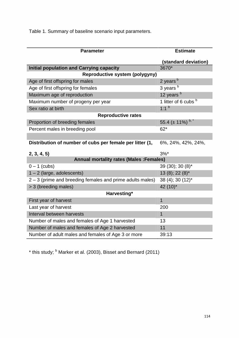
114
Table 1. Summary of baseline scenario input parameters.
Parameter Estimate
(standard deviation)
Initial population and Carrying capacity 3670*
Reproductive system (polygyny)
Age of first offspring for males 2 years b
Age of first offspring for females 3 years b
Maximum age of reproduction 12 years b
Maximum number of progeny per year 1 litter of 6 cubs b
Sex ratio at birth 1:1 b
Reproductive rates
Proportion of breeding females 55.4 (± 11%) b, *
Percent males in breeding pool 62*
Distribution of number of cubs per female per litter (1,
2, 3, 4, 5)
6%, 24%, 42%, 24%,
3%* Annual mortality rates (Males :Females)
0 – 1 (cubs) 39 (30); 30 (8)*
1 – 2 (large, adolescents) 13 (8); 22 (8)*
2 – 3 (prime and breeding females and prime adults males) 38 (4); 30 (12)*
> 3 (breeding males) 42 (10)*
Harvesting*
First year of harvest 1
Last year of harvest 200
Interval between harvests 1
Number of males and females of Age 1 harvested 13
Number of males and females of Age 2 harvested 11
Number of adult males and females of Age 3 or more
harvested
39:13
* this study; b Marker et al. (2003), Bisset and Bernard (2011)
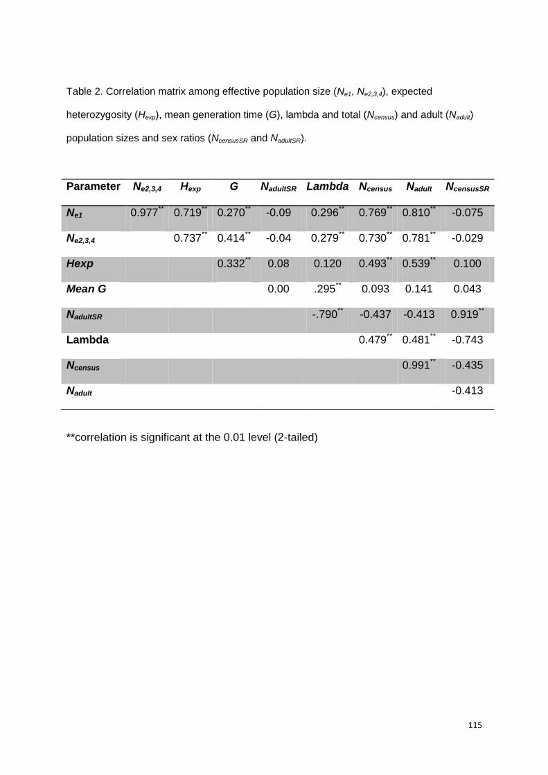
115
Table 2. Correlation matrix among effective population size (Ne1, Ne2,3,4), expected
heterozygosity (Hexp), mean generation time (G), lambda and total (Ncensus) and adult (Nadult)
population sizes and sex ratios (NcensusSR and NadultSR).
**correlation is significant at the 0.01 level (2-tailed)
Parameter Ne2,3,4 Hexp G NadultSR Lambda Ncensus Nadult NcensusSR
Ne1 0.977** 0.719** 0.270** -0.09 0.296** 0.769** 0.810** -0.075
Ne2,3,4 0.737** 0.414** -0.04 0.279** 0.730** 0.781** -0.029
Hexp 0.332** 0.08 0.120 0.493** 0.539** 0.100
Mean G 0.00 .295** 0.093 0.141 0.043
NadultSR -.790** -0.437 -0.413 0.919**
Lambda 0.479** 0.481** -0.743
Ncensus 0.991** -0.435
Nadult -0.413
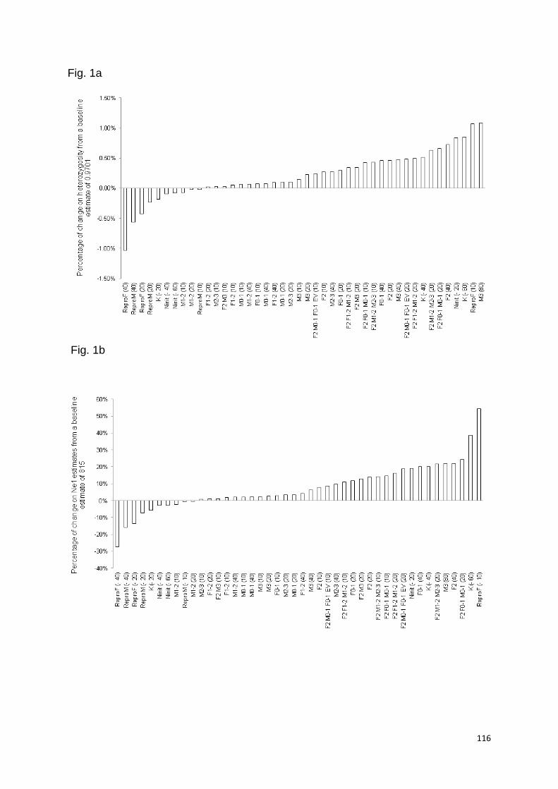
116
Fig. 1a
Fig. 1b
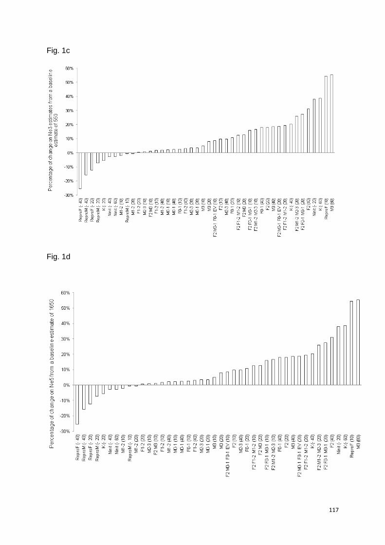
117
Fig. 1c
Fig. 1d

118
Fig. 1e
Fig. 1f
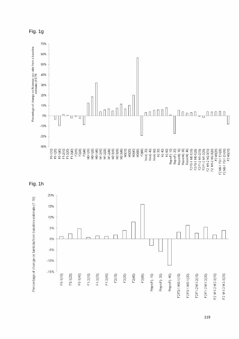
119
Fig. 1g
Fig. 1h
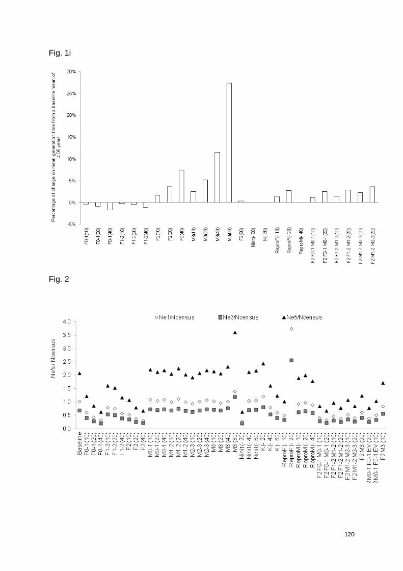
120
Fig. 1i
Fig. 2
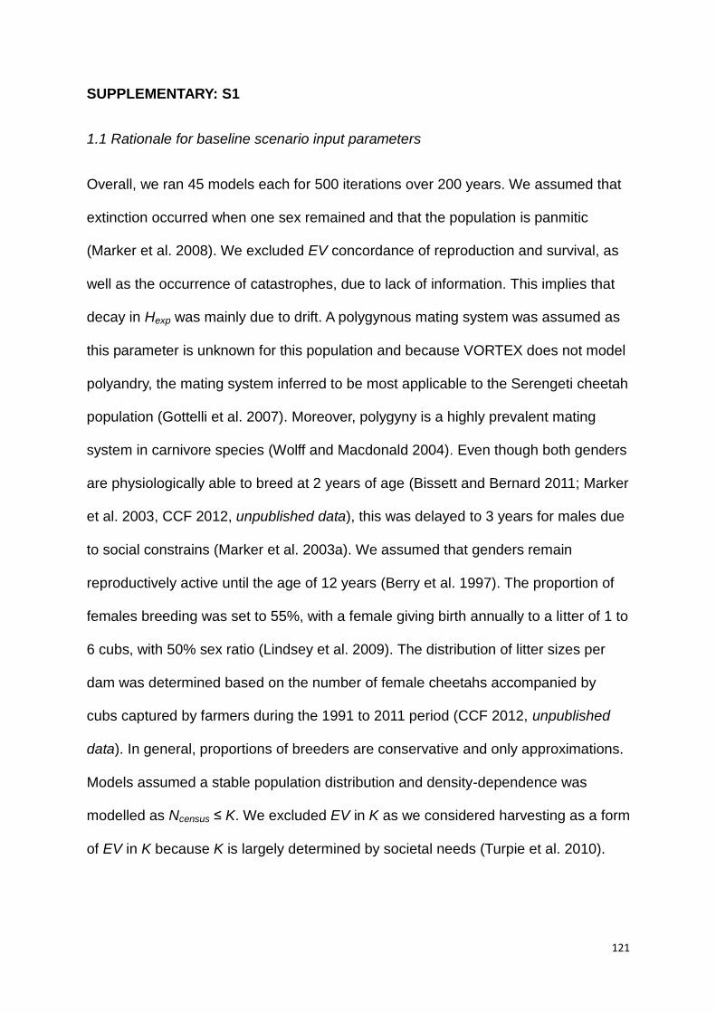
121
SUPPLEMENTARY: S1
1.1 Rationale for baseline scenario input parameters
Overall, we ran 45 models each for 500 iterations over 200 years. We assumed that
extinction occurred when one sex remained and that the population is panmitic
(Marker et al. 2008). We excluded EV concordance of reproduction and survival, as
well as the occurrence of catastrophes, due to lack of information. This implies that
decay in Hexp was mainly due to drift. A polygynous mating system was assumed as
this parameter is unknown for this population and because VORTEX does not model
polyandry, the mating system inferred to be most applicable to the Serengeti cheetah
population (Gottelli et al. 2007). Moreover, polygyny is a highly prevalent mating
system in carnivore species (Wolff and Macdonald 2004). Even though both genders
are physiologically able to breed at 2 years of age (Bissett and Bernard 2011; Marker
et al. 2003, CCF 2012, unpublished data), this was delayed to 3 years for males due
to social constrains (Marker et al. 2003a). We assumed that genders remain
reproductively active until the age of 12 years (Berry et al. 1997). The proportion of
females breeding was set to 55%, with a female giving birth annually to a litter of 1 to
6 cubs, with 50% sex ratio (Lindsey et al. 2009). The distribution of litter sizes per
dam was determined based on the number of female cheetahs accompanied by
cubs captured by farmers during the 1991 to 2011 period (CCF 2012, unpublished
data). In general, proportions of breeders are conservative and only approximations.
Models assumed a stable population distribution and density-dependence was
modelled as Ncensus ≤ K. We excluded EV in K as we considered harvesting as a form
of EV in K because K is largely determined by societal needs (Turpie et al. 2010).
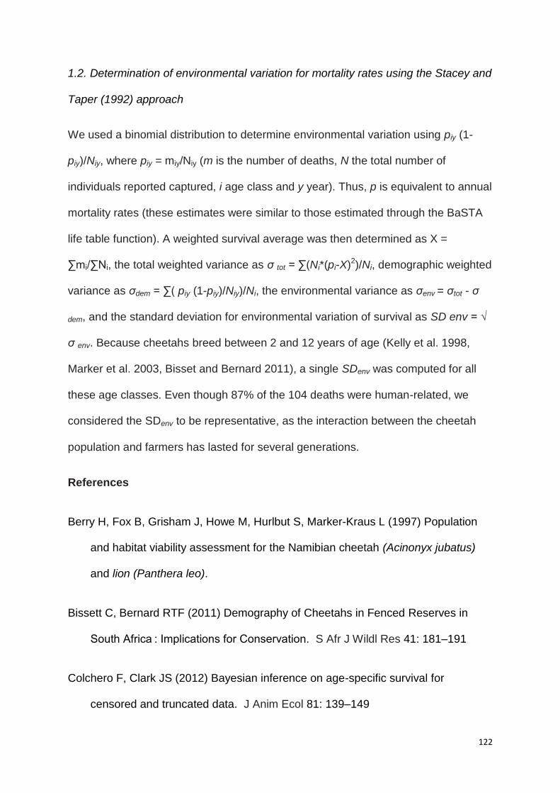
122
1.2. Determination of environmental variation for mortality rates using the Stacey and
Taper (1992) approach
We used a binomial distribution to determine environmental variation using piy (1-
piy)/Niy, where piy = miy/Niy (m is the number of deaths, N the total number of
individuals reported captured, i age class and y year). Thus, p is equivalent to annual
mortality rates (these estimates were similar to those estimated through the BaSTA
life table function). A weighted survival average was then determined as X =
∑mi/∑Ni, the total weighted variance as σ tot = ∑(Ni*(pi-X)2)/Ni, demographic weighted
variance as σdem = ∑( piy (1-piy)/Niy)/Ni, the environmental variance as σenv = σtot - σ
dem, and the standard deviation for environmental variation of survival as SD env = √
σ env. Because cheetahs breed between 2 and 12 years of age (Kelly et al. 1998,
Marker et al. 2003, Bisset and Bernard 2011), a single SDenv was computed for all
these age classes. Even though 87% of the 104 deaths were human-related, we
considered the SDenv to be representative, as the interaction between the cheetah
population and farmers has lasted for several generations.
References
Berry H, Fox B, Grisham J, Howe M, Hurlbut S, Marker-Kraus L (1997) Population
and habitat viability assessment for the Namibian cheetah (Acinonyx jubatus)
and lion (Panthera leo).
Bissett C, Bernard RTF (2011) Demography of Cheetahs in Fenced Reserves in
South Africa : Implications for Conservation. S Afr J Wildl Res 41: 181–191
Colchero F, Clark JS (2012) Bayesian inference on age-specific survival for
censored and truncated data. J Anim Ecol 81: 139–149
123
Colchero F, Jones OR, Rebke M (2012) BaSTA : an R package for Bayesian
estimation of age-specific survival from incomplete mark – recapture / recovery
data with covariates. MEE doi:10.1111/j.2041-210X.2012.00186.x
Gottelli D, Wang J, Bashir S, Durant, SM (2007) Genetic analysis reveals
promiscuity among female cheetahs. Proc R Soc B 274: 1993–2001
Hanssen L, Stander P (2004) Namibia large carnivore atlas. Predator Conservation
Trust, 1, 1 –12. Windhoek, Namibia
Kelly MJ, Laurenson MK, Fitzgibbon CD, Collins DA, Durant SM, Frame W, Bertram,
BCR et al. (1998) Demography of the Serengeti cheetah (Acinonyx jubatus)
population : the first 25 years. J Zool (Lond) 244: 473– 488
Marker L, Dickman, AJ, Jeo RM, Mills MGL, Macdonald DW (2003) Demography of
the Namibian cheetah , Acinonyx jubatus jubatus. Biol Cons. 114: 413–425.
Marker L, Wilkerson AJP, Sarno RJ, Marteson J, Breitenmoser-Würsten C, O’Brien,
SJ, Johnson WE (2008) Molecular Genetic Insights on Cheetah (Acinonyx
jubatus) Ecology and Conservation in Namibia. J Hered 99: 2–13
Stacey PB, Taper M (1992) Environmental variation and the persistence of small
populations. Ecol Appl 2: 18-29
Turpie AJ., Midgley G, Brown C, Barnes J, Pallett J, Desmet P, Tarr J, et al. (2010)
Climate Change Vulnerability and Adaptation Assessment for Namibia ’ s
Biodiversity and Protected. Windhoek, Namibia

124
Wolff JO, Macdonald DW (2004) Promiscuous females protect their offspring. TREE
19:127 – 134
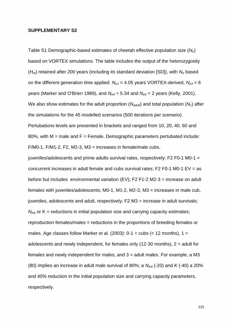
125
SUPPLEMENTARY S2
Table S1 Demographic-based estimates of cheetah effective population size (Ne)
based on VORTEX simulations. The table includes the output of the heterozygosity
(Het) retained after 200 years (including its standard deviation [SD]), with Ne based
on the different generation time applied: Ne1 = 4.05 years VORTEX-derived, Ne3 = 6
years (Marker and O'Brien 1989), and Ne4 = 5.34 and Ne5 = 2 years (Kelly, 2001).
We also show estimates for the adult proportion (Nadult) and total population (Nc) after
the simulations for the 45 modelled scenarios (500 iterations per scenario).
Pertubations levels are presented in brackets and ranged from 10, 20, 40, 60 and
80%, with M = male and F = Female. Demographic parameters pertubated include:
F/M0-1, F/M1-2, F2, M2-3, M3 = increases in female/male cubs,
juveniles/adolescents and prime adults survival rates, respectively; F2 F0-1 M0-1 =
concurrent increases in adult female and cubs survival rates; F2 F0-1 M0-1 EV = as
before but includes environmental variation (EV); F2 F1-2 M2-3 = increase on adult
females with juveniles/adolescents; M0-1, M1-2, M2-3, M3 = increases in male cub,
juveniles, adolescents and adult, respectively; F2 M3 = increase in adult survivals;
Ninit or K = reductions in initial population size and carrying capacity estimates;
reproduction females/males = reductions in the proportions of breeding females or
males. Age classes follow Marker et al. (2003): 0-1 = cubs (< 12 months), 1 =
adolescents and newly independent, for females only (12-30 months), 2 = adult for
females and newly independent for males, and 3 = adult males. For example, a M3
(80) implies an increase in adult male survival of 80%; a Ninit (-20) and K (-40) a 20%
and 40% reduction in the initial population size and carrying capacity parameters,
respectively.
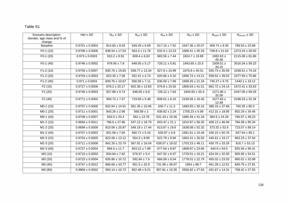
126
Table S1
Scenario description: Gender, age class and % of
change
Het ± SD Ne1 ± SD Ne3 ± SD Ne4 ± SD Ne5 ± SD Nadult ± SD Ncensus ± SD
Baseline 0.9701 ± 0.0004 814.65 ± 9.93 549.29 ± 6.69 617.15 ± 7.52 1647.36 ± 20.07 409.74 ± 9.35 789.53 ± 23.68
F0-1 (10) 0.9708 ± 0.0006 838.54 ± 17.53 563.3 ± 11.78 632.9 ± 13.23 1689.41 ± 35.33 708.8 ± 21.63 1373.24 ± 26.93
F0-1 (20) 0.973 ± 0.0003 910.2 ± 9.91 608.4 ± 6.63 683.56 ± 7.44 1824.7 ± 19.88 1082.63 ± 45.48
2115.08 ± 81.86
F0-1 (40) 0.9746 ± 0.0002 978.06 ± 7.8 648.05 ± 5.17 728.11 ± 5.81 1943.65 ± 15.5 1509.51 ± 34.15
3016.34 ± 59.23
F1-2 (10) 0.9706 ± 0.0007 830.76 ± 19.83 558.77 ± 13.34 627.8 ± 14.99 1675.8 ± 40.01 535.73 ± 35.59 1038.51 ± 74.16
F1-2 (20) 0.9703 ± 0.0003 823.35 ± 7.06 552.41 ± 4.74 620.66 ± 5.32 1656.74 ± 14.21 558.52 ± 39.52 1077.59 ± 70.86
F1-2 (40) 0.971 ± 0.0004 849.76 ± 10.67 566.59 ± 7.11 636.59 ± 7.99 1699.26 ± 21.34 745.27 ± 9.75 1440.1 ± 19.12
F2 (10) 0.9727 ± 0.0006 878.2 ± 20.17 602.38 ± 13.83 676.8 ± 15.55 1806.63 ± 41.51 862.72 ± 24.14 1672.41 ± 33.63
F2 (20) 0.9746 ± 0.0003 927.88 ± 9.74 648.05 ± 6.8 728.12 ± 7.64 1943.65 ± 20.4 1271.86 ± 32.09
2447.09 ± 69.29
F2 (40) 0.9771 ± 0.0002 993.72 ± 7.57 719.69 ± 5.48 808.61 ± 6.15 2158.56 ± 16.45 1677.65 ± 12.48
3198.23 ± 31.34
M0-1 (10) 0.9707 ± 0.0005 832.54 ± 14.91 561.35 ± 10.06 630.7 ± 11.3 1683.55 ± 30.16 388.16 ± 37.68 760.35 ± 80.3
M0-1 (20) 0.9711 ± 0.0001 843.26 ± 2.96 568.58 ± 2 638.82 ± 2.24 1705.23 ± 5.99 412.31 ± 18.95 802.29 ± 34.46
M0-1 (40) 0.9708 ± 0.0007 833.5 ± 20.4 562 ± 13.76 631.43 ± 15.46 1685.49 ± 41.26 384.5 ± 24.29 766.57 ± 48.23
M1-2 (10) 0.9694 ± 0.0011 796.6 ± 27.86 537.12 ± 18.79 603.47 ± 21.1 1610.87 ± 56.35 408.13 ± 46.94 784.08 ± 85.34
M1-2 (20) 0.9699 ± 0.0009 810.06 ± 25.87 546.19 ± 17.44 613.67 ± 19.6 1638.08 ± 52.32 373.32 ± 52.6 723.57 ± 89.14
M1-2 (40) 0.9707 ± 0.0003 831.58 ± 7.65 560.71 ± 5.16 629.97 ± 5.8 1681.61 ± 15.48 430.15 ± 50.76 827.64 ± 95.1
M2-3 (10) 0.9704 ± 0.0005 822.09 ± 13.12 554.3 ± 8.85 622.79 ± 9.94 1662.41 ± 26.55 445.61 ± 19.17 863.23 ± 37.54
M2-3 (20) 0.9711 ± 0.0008 842.26 ± 23.79 567.91 ± 16.04 638.07 ± 18.02 1703.23 ± 48.11 430.75 ± 33.26 816.7 ± 53.13
M2-3 (40) 0.9727 ± 0.0004 894.5 ± 11.7 603.12 ± 7.89 677.64 ± 8.87 1808.87 ± 23.66 444.6 ± 54.5 825.94 ± 95.41
M3 (10) 0.9715 ± 0.0003 834.64 ± 7.82 576.67 ± 5.4 647.92 ± 6.07 1729.51 ± 16.21 424.33 ± 32.05 805.95 ± 54.51
M3 (20) 0.9723 ± 0.0004 835.86 ± 10.72 592.84 ± 7.6 666.08 ± 8.54 1778.01 ± 22.79 455.02 ± 23.53 860.01 ± 32.98
M3 (40) 0.9747 ± 0.0012 866.66 ± 43.77 651.5 ± 32.9 731.99 ± 36.97 1954 ± 98.7 461.28 ± 12.51 840.75 ± 27.81
M3 (80) 0.9806 ± 0.0002 993.14 ± 10.73 852.48 ± 9.21 957.81 ± 10.35 2556.92 ± 27.63 431.67 ± 14.31 708.42 ± 27.55
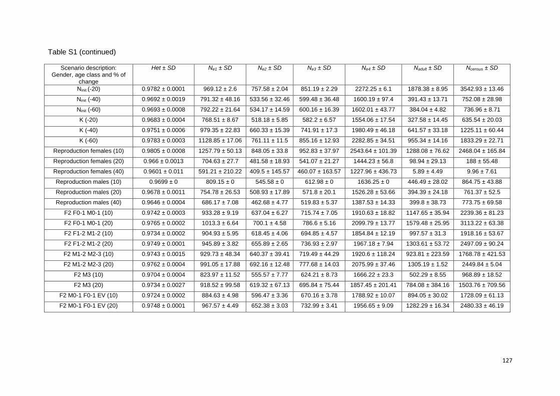
127
Table S1 (continued)
Scenario description: Gender, age class and % of
change
Het ± SD Ne1 ± SD Ne2 ± SD Ne3 ± SD Ne4 ± SD Nadult ± SD Ncensus ± SD
Ninit (-20) 0.9782 ± 0.0001 969.12 ± 2.6 757.58 ± 2.04 851.19 ± 2.29 2272.25 ± 6.1 1878.38 ± 8.95 3542.93 ± 13.46
Ninit (-40) 0.9692 ± 0.0019 791.32 ± 48.16 533.56 ± 32.46 599.48 ± 36.48 1600.19 ± 97.4 391.43 ± 13.71 752.08 ± 28.98
Ninit (-60) 0.9693 ± 0.0008 792.22 ± 21.64 534.17 ± 14.59 600.16 ± 16.39 1602.01 ± 43.77 384.04 ± 4.82 736.96 ± 8.71
K (-20) 0.9683 ± 0.0004 768.51 ± 8.67 518.18 ± 5.85 582.2 ± 6.57 1554.06 ± 17.54 327.58 ± 14.45 635.54 ± 20.03
K (-40) 0.9751 ± 0.0006 979.35 ± 22.83 660.33 ± 15.39 741.91 ± 17.3 1980.49 ± 46.18 641.57 ± 33.18 1225.11 ± 60.44
K (-60) 0.9783 ± 0.0003 1128.85 ± 17.06 761.11 ± 11.5 855.16 ± 12.93 2282.85 ± 34.51 955.34 ± 14.16 1833.29 ± 22.71
Reproduction females (10) 0.9805 ± 0.0008 1257.79 ± 50.13 848.05 ± 33.8 952.83 ± 37.97 2543.64 ± 101.39 1288.08 ± 76.62 2468.04 ± 165.84
Reproduction females (20) 0.966 ± 0.0013 704.63 ± 27.7 481.58 ± 18.93 541.07 ± 21.27 1444.23 ± 56.8 98.94 ± 29.13 188 ± 55.48
Reproduction females (40) 0.9601 ± 0.011 591.21 ± 210.22 409.5 ± 145.57 460.07 ± 163.57 1227.96 ± 436.73 5.89 ± 4.49 9.96 ± 7.61
Reproduction males (10) 0.9699 ± 0 809.15 ± 0 545.58 ± 0 612.98 ± 0 1636.25 ± 0 446.49 ± 28.02 864.75 ± 43.88
Reproduction males (20) 0.9678 ± 0.0011 754.78 ± 26.53 508.93 ± 17.89 571.8 ± 20.1 1526.28 ± 53.66 394.39 ± 24.18 761.37 ± 52.5
Reproduction males (40) 0.9646 ± 0.0004 686.17 ± 7.08 462.68 ± 4.77 519.83 ± 5.37 1387.53 ± 14.33 399.8 ± 38.73 773.75 ± 69.58
F2 F0-1 M0-1 (10) 0.9742 ± 0.0003 933.28 ± 9.19 637.04 ± 6.27 715.74 ± 7.05 1910.63 ± 18.82 1147.65 ± 35.94 2239.36 ± 81.23
F2 F0-1 M0-1 (20) 0.9765 ± 0.0002 1013.3 ± 6.64 700.1 ± 4.58 786.6 ± 5.16 2099.79 ± 13.77 1579.48 ± 25.95 3113.22 ± 63.38
F2 F1-2 M1-2 (10) 0.9734 ± 0.0002 904.93 ± 5.95 618.45 ± 4.06 694.85 ± 4.57 1854.84 ± 12.19 997.57 ± 31.3 1918.16 ± 53.67
F2 F1-2 M1-2 (20) 0.9749 ± 0.0001 945.89 ± 3.82 655.89 ± 2.65 736.93 ± 2.97 1967.18 ± 7.94 1303.61 ± 53.72 2497.09 ± 90.24
F2 M1-2 M2-3 (10) 0.9743 ± 0.0015 929.73 ± 48.34 640.37 ± 39.41 719.49 ± 44.29 1920.6 ± 118.24 923.81 ± 223.59 1768.78 ± 421.53
F2 M1-2 M2-3 (20) 0.9762 ± 0.0004 991.05 ± 17.88 692.16 ± 12.48 777.68 ± 14.03 2075.99 ± 37.46 1305.19 ± 1.52 2449.84 ± 5.04
F2 M3 (10) 0.9704 ± 0.0004 823.97 ± 11.52 555.57 ± 7.77 624.21 ± 8.73 1666.22 ± 23.3 502.29 ± 8.55 968.89 ± 18.52
F2 M3 (20) 0.9734 ± 0.0027 918.52 ± 99.58 619.32 ± 67.13 695.84 ± 75.44 1857.45 ± 201.41 784.08 ± 384.16 1503.76 ± 709.56
F2 M0-1 F0-1 EV (10) 0.9724 ± 0.0002 884.63 ± 4.98 596.47 ± 3.36 670.16 ± 3.78 1788.92 ± 10.07 894.05 ± 30.02 1728.09 ± 61.13
F2 M0-1 F0-1 EV (20) 0.9748 ± 0.0001 967.57 ± 4.49 652.38 ± 3.03 732.99 ± 3.41 1956.65 ± 9.09 1282.29 ± 16.34 2480.33 ± 46.19

128
Chapter IV
129
Using remote camera traps for surveying and monitoring trends in abundance
and density: a case study of a cheetah population in north-central Namibia
Author list:
Ezequiel Chimbioputo Fabiano 1, 2
Matti Nghikembua 2
Eduardo Eizirik 1
Laurie Marker 2
Affiliations:
1. Laboratório de Biologia Genômica e Molecular, Faculdade de Biociências,
Pontifícia Universidade Católica do Rio Grande do Sul, Porto Alegre, RS 90619-900,
Brazil
2. Cheetah Conservation Fund, PO Box 1755, Otjiwarongo, Namibia. Fax: 264 67
306247
Email addresses:
130
Corresponding authors:
Ezequiel C. Fabiano
Cheetah Conservation Fund,
P.O. Box 1755, Otjiwarongo, Namibia.
Fax: 264 67 306247
Running title:
Cheetah population dynamics assessed with remote camera traps.
131
SUMMARY
1. The ability to monitor population abundance and density is necessary in
assessing trends, while providing vital information for designing of
conservation actions. This is a complex task, especially for species such as
the cheetah Acinonyx jubatus due to behavioural and ecological aspects.
Consequently, current population estimates are often based on methods that
do not account for sampling biases such as imperfect detection. We
investigated the use of remote camera trapping (RCT) with classical and
spatial capture recapture (SCR) models for monitoring the abundance and
density of a cheetah population while exploring the utilisation patterns of scent
marking sites in north-central Namibia.
2. We analysed RCT data collected mostly at scent marking sites for 10 surveys
conducted between 2005 and 2011, each lasting three months. In addition,
four camera-detected male cheetahs were fitted with GSM collars to assess
home range overlap in relation to the camera trap polygon.
3. Overall, 54 unique cheetahs were identified (8 ± 4 individuals per survey),
which were predominantly nocturnal with some crepuscular behaviour. We
observed high fidelity to scent stations for up to 4 years by resident cheetahs,
with new recruits displaying spatial and temporal patterns that were similar to
their predecessors’.
4. Density estimates based on effective sampling areas were determined using
classical methods such as the full Mean Maximum Distance Moved and the
home range radius or sum of home range sizes, which were similar to SCR-
based estimates. However, SCR multi-survey density estimates were more
132
consistent and ranged between 5 and 16 km-3, with a coefficient of variation of
11.7%. Further, our data provide some evidence suggesting that male density
may be regulated by home range dynamics, as it remained similar only in
periods of social stability.
5. In addition to reporting robust longitudinal density estimates for cheetahs
using RCT with SCR methods, this study provides information on behavioural
aspects such as spatial overlap and utilisation of scent marking sites. Overall,
we found that the techniques applied here hold great promise for surveying
cheetah populations in general, and highlight the need for sampling large
areas in order to obtain reliable estimates.
Key-words: camera trapping, population dynamics, scent marking sites, spatial
capture recapture, spatial and temporal activity patterns.
133
Introduction
The cheetah (Acinonyx jubatus jubatus, Schreber, 1775) is classified as a vulnerable
species by the IUCN (Durant et al. 2008). Currently, Namibia holds the largest free-
ranging population of cheetahs (Durant et al. 2008), of which 90% occurs on
livestock and game farmlands where cheetah dominant competitors such as lions
(Panthera leo) and spotted hyenas (Crocuta crocuta) have been extirpated (Marker-
Kraus et al. 1996; Durant 2000). Thus, unlike in protected areas, where cheetahs live
at low density due to interspecific competition (Caro 1994; Durant 2000),
indiscriminate removals are considered a major factor affecting the population
dynamics in areas where interspecific competition is minimal due to the absence of
lions and spotted hyenas (Marker et al. 2003, 2007). In addition, anthropogenic
factors tend to reduce and slow down growth rate of carnivores (Creel and Rotella
2010; Sparkman, Waits and Murray 2011; Wich et al. 2011). Other factors
influencing population dynamics include habitat, prey availability, droughts, social
organization (Packer et al. 2005), home range or territoriality dynamics, spatial use
patterns and dispersal (Odum 2004; Gorman and Trowbridge 1989). These
mechanisms affect the reproduction patterns, hence the population effective size
(Ne) (Mayer and Pasinelli 2013). The extent to which these mechanisms are
prevalent in the Namibian population is largely unknown.
RCT has been used as a means of effectively estimating abundance and
density of a variety of cryptic species including tigers (Panthera tigris) (Karanth et al.
2006), leopards (P. pardus), brown hyena (Hyaena brunnea), aardwolf (Proteles
cristata) (O'Brien and Kinnaird 2011) and cheetahs (Marker, Fabiano and
Nhikembua 2008). However, in a few cases, RCT has been utilized to determine
long-term population trends (Karanth et al. 2006; Barlow et al. 2009). Only a single
134
study has assessed long-term trends on cheetah through distance sampling (Durant
et al. 2011). However, distance sampling may be unsuitable for surveying cheetahs
in areas outside protected area (e.g. in Namibia) due to the species ecological
behaviour (e.g. roam across vast home ranges, be elusive, skittish) (Gese 2001) or
due to limited visibility.
Density-related RCT studies often estimate effective sampling areas (ESA)
using a variety of ad hoc buffer estimates, determined using the half and full mean
maximum distance moved by all animals recaptured at multiple stations and the
home range (HR) radius of individuals radio collared simultaneously as RCT surveys
are ongoing or based on the literature (Soisalo and Calvacanti 2006; Marker,
Fabiano and Nghikembua 2008). The application of these approaches is problematic
as these buffer estimates may lack a formal relationship to HRs or territories of the
sampled individuals (Gardner et al. 2010a). Furthermore, these approaches fail to
capture the heterogeneity in the probability of detection caused by populations being
geographically open as sampling areas are often smaller than camera-detected
individual's HRs (White et al. 1982). Consequently, these shortfalls often yield
positively biased estimates as the movements patterns of individuals in relation to
camera trap layout are underestimated (Marker, Fabiano and Nghikembua 2008;
Gerber, Karpanty and Kelly 2012 but see Balme, Hunter and Slotow 2009). Other
surveying techniques previously used to estimate cheetah abundance and density in
Namibia are also affected by these sources of error and others (e.g. double counting,
imperfect detection). Techniques include radio tracking (Morbasch 1975; Marker
2002), spoor tracking (Fabiano 2007) and questionnaires, interviews and sighting
reports (Myers 1975; Hanssen and Stander (2004). Ultimately, the impossibility of
135
estimating population trends in Namibia is caused by the lack of a reliable, precise
estimate of abundance and density.
In order to circumvent these and other issues that may affect the reliability of
density estimations, spatial capture recapture models (SCR) have been developed
and continue to be refined (Efford 2004; Royle and Young 2008; Borchers and Efford
2008; Royle et al. 2009; Efford and Fewster 2012; Royle et al. 2013). SCR
approaches account for individual heterogeneity by incorporating the auxiliary spatial
information about where individuals are captured when constructing capture
histories, thus making full use of the information from camera data sets (Royle et al.
2009). As such, detection rates are a function of the distance between the camera
trap locations and the centre of an individual’s HR (Efford 2004). Consequently, this
parameterization allows for a direct determination of the ESA thus obtaining less
biased estimates. Overall, we compared non-spatial and SCR approaches on
cheetahs.
Cheetahs scent marks terminate mounds and certain trees with urine and less
often with faeces (Eaton 1970; Marker-Kraus et al. 1996). Eaton (1970) suggested
that for cheetahs in the Serengeti, scent marking is a "time-plan" by which
conspecifics individuals with overlapping HR coexist with minimal risk of direct
encounter, through intensive marking, as it is unviable for them to establish exclusive
territories given their extensive HR. This time plan to be effective requires at higher
scent marking frequency (Eaton 1970) and at strategic sites in order to maximize
encounter rates (Gorman and Trowbridge 1989). Male cheetahs in Namibia visit a
scent-marking site on average every six (± 9) days (Marnewick, Funston and
Karanth 2006; Marker, Fabiano and Nhikembua 2008). Scent marking is also
involved on advertisement of reproductive status (Smith et al. 1989), territory
136
demarcation and defence (Gese and Ruff 1997; Sillero-Zubiri and Macdonald 1998),
foraging orientation including food resources, maintaining social structure (Revilla
and Palomares 2002; Gorman and Trowbridge 1989), HR familiarity to cubs by
mothers (Seidensticker et al. 1973). However, the distribution and visitation pattern
(utilization pattern) of scent marking sites in relation to individual HR is largely
unknown for the Namibian cheetah population.
Here, we used a combination of a six years remote camera trap (RCT) placed
mostly at scent marking sites and radio telemetry data sets, to provide new insights
into processes affecting a cheetah population (fine scale level) while assessing
trends in abundance and density based on a robust systematic approach. Specific
objectives were to (i) determine the population structure over time, (ii) describe the
spatial utilisation patterns of scent marking sites that are important for ecological and
behavioural purposes, and (iii) compare cheetah densities estimated using non-
spatial and SCR methods. Furthermore, we discuss the pros and cons of using
spatial vs. non-spatial methods for density estimation.
Materials and methods
STUDY AREA
We conducted this study primarily on the Cheetah Conservation Fund property,
located in the Waterberg Conservancy in north-central Namibia (20°28'56"S
17°2'24"E, Fig. 1). The area is semi-arid and falls between 400 mm and 500 mm
rainfall isopleths (Barnard 1998). Namibia is considered to have three seasons:
summer, intermediate and winter (Berry 1980). The area falls within the thornbush,
tree and woodland savanna vegetation zone (Geiss 1971) with prevalent occurrence
of bush encroachment (Barnard 1998). Livestock (primarily cattle and smallstock)
137
and wildlife, including fenced game farms, eco-tourism and trophy hunting are the
primary forms of land use (Marker-Kraus et al. 1996). The area harbours a diversity
of ungulates including the oryx (Oryx gazella), kudu (Tragelaphus strepsiceros),
eland (Taurotragus oryx), springbok (Antidorcas marsupialis), and steenbok
(Raphicerus campestris) among others, and sympatric carnivores including brown
hyena, caracal (Caracal caracal), black-backed jackal (Canis mesomelas), and
leopard (nomenclature for species names follows Estes 1991).
STUDY DESIGN AND DATA COLLECTION
RCT surveys were conducted annually for three months from 2005 to 2009, and then
continuously between July 2010 and December 2011, encompassing an average
area of 377 km2 (SD + 41.15 km2) (Fig. 1, S1, Table 1). Although Namibia is
considered to have three seasons, for the purpose of this study, surveys were
grouped into two main seasons, Summer (Nov – May) and Winter (June – Oct).
Overall, five surveys each were conducted during the summer and winter seasons.
During the course of the study, 32 different sampling stations were deployed (15 to
19 per survey, Table 1). Sampling effort was similar across surveys despite
relocating or terminating stations that failed to detect a cheetah in a survey in order
to increase detection probabilities (as suggested by Karanth and Nichols [2002]).
Sixty-three percent (n = 20) of the stations were located at scent marking posts and
19% (n = 6) either next to roads/fence lines and in close proximity to cheetah captive
facilities. Inter-camera distances were on average 17 km (± 9.24 km), a distance that
falls within the HR radius (i) of four radio collared individuals (3 to 10 km) (this study)
and (ii) of 22.95 km (n = 41, 26 males and 15 females) from a previous long-term
telemetry study conducted in the area (Marker et al. 2008). This spacing and
geographical distribution of cameras ensured that no animal HR was unsampled
138
(Karanth and Nichols 2002). We used DeerCamTM DC200 (DeerCam, Park Falls,
WI, USA) and Bushnell Trophy (Trophy Cam 2009, Kansas, USA) cameras from
2005 to 2009 and 2010 through to 2011, respectively. In 2008, one station had a
Moultrie M60 digital camera (Georgia, USA). We placed two cameras per station,
mounted ca. 75 cm above the ground and 5 m apart. Cameras sites were checked
for functionality, as well as to change film/memory card and/or batteries on average
once a week (range of 2 to 7 days). For data management, cheetah pictures from
developed films were logged into an Excel database, while an automatic storage
software was used for memory cards (Harris et al. 2010).
One of the non-spatial buffer estimates used to determine ESA was the radius
of a 95% minimum convex polygon (MCP) home range, as determined by radio
telemetry. To allow this assessment, four RCT-detected male cheetahs (two single
males and two males belonging to two coalitions of two males each) were captured,
immobilized and fitted with Global System for Mobile communications (GSM) collars
in 2007. Collars took three to five Global Positioning System (GPS) readings per
day, lasting for a maximum of nine months. Immobilization procedures followed
those of Marker et al. (2003). Cheetahs were released shortly after capture as close
as possible to the capture site, in order to minimize unavailability for detection by
cameras. These cheetahs are referred to by unique numbers (i.e. AJU#, Table 2).
Data analysis
139
CAPTURE SUCCESS, DEMOGRAPHIC STRUCTURE AND SPATIAL USE
PATTERNS OF SCENT MARKING SITES
To be consistent with our previous work and adhere to recommendations of
sampling periods to uphold the closure assumption (Karanth and Nichols 2002;
Marker, Fabiano and Nghikembua 2008), we stratified the continuous effort (i.e.
2010 through 2011 data set) into six surveys, of 90 days each. We identified
individual cheetahs manually based on unique spot patterns, which remain unaltered
throughout their lifetime (Caro and Durant 1991). Gender was determined using cues
such as the presence of visible genitals, ear tag position (i.e. right for males and left
for females) or accompanying cubs. A cheetah was classified as either a cub (≤ 1
years old) or adult (> 1 year old); male or female; or as single, member of male
coalition or breeding female (i.e. with accompanying cubs). Individuals were also
classified as resident if they were captured during at least two consecutive inter-
annual surveys (i.e. the six surveys spaced equally apart) or during two consecutive
stratified surveys within the 2010 - 2011 continuous survey (Caro and Collins 1987;
Barlow et al. 2009). All other individuals were treated as non-resident as non-
resident cheetahs tend to remain no more than a few days in the same area (Bothma
and Walker 1999). Likewise, we considered a camera site to be an integral
component of an individual’s HR if it was visited continuously on all surveys in which
the individual was detected. This consideration was limited to residents.
We explored the distribution and density of camera traps sites in relation to
GSM HR. HR were calculated as core (45% Kernel), intermediate (80%) and border
(> 80%) (Castillo, Lucherini and Casanave 2011).
140
POPULATION ESTIMATION: NON-SPATIAL CAPTURE-RECAPTURE
We used data on identified individuals for estimating and assessing trends in
abundance and density. The programs CloseTest and CAPTURE (Otis et al. 1978;
Rexstad and Burnham 1991) were used to test the closure assumption, with the
latter also being employed to estimate abundance (N). For individual capture
histories, we set an occasion to equal six sampling days. Evidence for the presence
of transients was determined through program U-CARE2.2 (Choquet et al. 2005).
Non-spatial density estimates were computed by dividing abundance by the size of
the four ESAs. ESAs were determined by buffering the camera trap MCP with the: (i)
full mean maximum distance traversed by individuals captured on multiple stations
(FMMDM); (ii) mean radius of the 95% MCP HRs of four GSM collared males (GSM-
ESA); (iii) mean radius of the 95% MCP HRs of 41 individuals (26 males and 15
females) VHF collared reported by Marker et al. (2008) (VHF-ESA). The FMMDM
was used as opposed to the half MMDM, as our previous work showed the latter to
be underestimated resulting in unrealistic density estimates (Marker, Fabiano and
Nhikembua 2008 see also Soisolo and Calvacanti 2006). Lastly, we also used the
size of the 95% MCP for the GSM collar-derived HRs as ESA (GSM-polygon). The
latter was considered a minimum density estimate. The 95% MCP, Kernel HR sizes
and range overlaps were computed using the HR and Spatial Analysis extension of
ArcView 3.2 (version 3.2) and ArcGis 9.3 (ESRI, Redlands, CA, USA) and HR radius
as Area = п r2, with r being the radius. ESA computations were also conducted using
this software. HR asymptotes were determined using ABODE (Laver 2005). For the
FMMDM, a single distance value was used for coalitions, as no evidence supporting
spatio-temporal separation of male coalitions was found for the study area in
141
Namibia. Naive standard errors for D were calculated by dividing standard error (SE)
of N by the ESA.
POPULATION ESTIMATION: BAYESIAN SPATIAL CAPTURE-RECAPTURE
We also used the Bayesian hierarchical R package SPACECAP 1.0.5 for SCR
analysis that accounts for imperfect detection and makes use of the geographic
locations of where individuals are captured to infer detection probabilities
(Gopalaswamy et al. 2012). We set state-space S to 6158 km2 (i.e. the area of the
camera trap array buffered with 22.95 km, the HR radius from Marker et al. 2008)
with a 3 x 3 km grid resolution. Both the grid resolution and S size are based on prior
knowledge of animal movement ranges and HR sizes (Marker et al. 2008; this
study). Density results were not affected by S specification, as observed on trials
with smaller polygons of similar or finer grid resolutions (e.g. 1430 km2, 2848 km2,
grids of 0.5 km, 1.5 km).
We used a Markov Chain Monte Carlo (MCMC) of 100,000 iterations with a
burn-in of 10% of the total samples, and thinned every 10 steps, as well as
incorporating the following features: data augmentation to 60 or 90 (M); trap
response; half-normal detection function; and Bernoulli's encounter model. We used
the default uninformative priors for all model parameters (i.e. σ, λ0, psi, and gamma)
and standardized density estimates to 1000 km2. We converted sigma (σ, animal
range) and lambda (λ0, baseline encounter rate) into an equivalent 95% home-range
radius and individual capture probability, respectively, through qchisq ((0.95,2)
0.5)*(σ) and 1 - exp (-λ0) (Noss et al. 2012). Underlying this mathematical conversion
is the assumption that HRs follows a bivariate normal distribution (Royle et al. 2009).
142
Estimates were considered to be significantly different at α = 0.05, if their 95%
CIs did not overlap by more than half (Cumming and Finch 2005; Noss et al. 2012).
Means are presented with standard deviation unless stated otherwise.
Results
CAPTURE SUCCESS, DEMOGRAPHIC STRUCTURE AND PATTERNS
Table 1 presents a summary of the sampling effort per survey for the 10 surveys
conducted between 2005 and 2011. Up to 32 stations were active at some stage
during the study (mode of 15 per survey) with 22% being active during all 10
surveys. This sampling effort resulted in 13770 (1377 ± 120) trap-nights and 2596
(260 ± 78) usable cheetah photographs per survey. While this estimate of sampling
effort does not account for cameras failures, seldom were both cameras on a site
non-functional. Fifty-four unique individuals were identified across the 10 surveys,
including two females released into the study area as part of CCF’s management
actions (Table 1). Two potentially additional individuals were detected on different
surveys, but discarded as it was not possible to ascertain their identity. Of the 54
individuals, 39 were adults and 15 were cubs. The majority of adult were males, 32
versus 7 females, with a consistent biased male sex ratio across surveys (Fig. 2b).
There was only one individual for which the sex could not be determined. Captured
adult males were mostly single (68%) whereas 32% occurred in coalitions. For three
males, it was possible to infer the age of death: the members of a coalition of two
(AJU1459 and 1460) died at the age of 5 and 6 years and a member of another
coalition (AJU1542) at 6 years (Table 2). The AJU1542 coalition member was still
alive at the end of 2011. While AJU1542 died in the midst of the fifth survey,
AJU1459 and 1460 died outside of any sampling period and a year apart (i.e. 2006
and 2007, respectively). As for females, all but one had accompanying cubs, with a
143
mean litter size of 3 ± 1.2. With respect to seasonal patterns, males were captured
throughout the surveys (usually including multiple recaptures), while females showed
a trend for increased capture probability in the summer (10 out of 15
capture/recapture events). Females tended to be captured only once, with only five
cases of recapturing.
On average 8 ± 4 (coefficient of variation 15%) individuals were captured per
survey (Table 1), with capture saturation occurring on average 7 (± 3) occasions
(approximately 44 days as) after the start of the survey (Fig. 3). Although saturation
occurred on average earlier in winter (7 ± 2 occasions) than in summer (8 ± 4
occasions), this difference was not statistically significant (t = 0.47, d.f. = 8, P =
0.65). Overall, capture rates declined as the study progressed, with non-resident
adults and cubs driving fluctuations in abundance.
TEMPORAL AND SPATIAL UTILISATION PATTERNS OF CHEETAHS BASED ON
RCT DATA
Temporal and spatial patterns of use of areas surveyed by camera traps by resident
cheetahs are presented in Table 2 and Fig. 4. The majority of detected individuals
were non-residents (77% of 39 adults). On average a cheetah was captured every 5
days (± 8), with residents (n = 7) being captured significantly more frequently than
non-residents (U = 14202, P < 0.01). When seasons were assessed separately, the
median time between captures was significantly different between residents and
non-residents in the summer (2 and 7 days, respectively; U = 4652, P < 0.01), and in
winter (2 and 6 days, respectively; U =2559 P < 0.01). When resident and non-
resident cheetahs were assessed separately, no significant difference was observed
in the summer capture interval (resident: 3.6 ± 6.5 days in summer and 2.5 ± 4.3
144
days in winter< U = 30598, P > 0.05; non-residents: 9.6 ± 11 days in summer and
15.6 ± 17 days in winter; U = 376, P > 0.05).
A certain level of spatial organization was deduced based on the distribution
of resident cheetah detections (Table 2). Clusters based on captures occurred
around stations 3 - 5, stations 10-12, and stations 14, 15 and 17 (Table 2). These
stations were in closer proximity to one another (Fig. 1). While some stations were
used within and across surveys by different individuals (e.g. stations 12, 14, 15, 17),
other were used either once or infrequently by different social groups (e.g. station
11). Utilisation patterns remained similar even after a turnover in resident individuals
occurred. For example, the activity centres for AJU1537 and 1538 were very similar
to those of their predecessors (i.e. AJU1459 and 1460), with these social groups
95% MCP overlapping by at least 35% (Table 2, Fig. 4). Likewise, utilisation patterns
of AJU1533 were similar to those of AJU1542 and 1543, with an overlap of two years
in their presence (Table 2). On the other hand, no new individuals were detected at
stations visited by M1 from 2007 until 2010-2 and 2011-2 when AJU1543 was
detected once at stations 3 and 5, respectively (Table 2). Overall, multi-year
detections per station ranged from six to 48 months (31 ± 16.3 months).
SPATIAL UTILISATION PATTERNS OF CHEETAHS BASED ON TELEMETRY
DATA
The spatial organization based on the GSM data was in agreement with that
retrieved by RCT data, whereby HRs for AJU1533, 1537 and 1459 encompassed the
camera sites where these individuals where detected (Fig. 1, Table 2). On average
741 fixes (± 695) were recorded over a period of 70 to 226 days (129 ± 68). The high
variation in fixes was a result of AJU1533 having 1763 fixes while the remaining
individual fixes ≤ 510 (TABLE S2). Despite the limited monitoring period all
145
individuals HRs reached asymptotes (AJU 1537 at 66 pts, AJU 1533 at 121 pts, AJU
1459 at 129 pts, and AJU 1536 at 144 pts) corroborating their status of residents.
The minimum average 95% MCP and Kernel HR size for the four individuals
were 269 ± 238.4 km2 and 126.5 ± 170.4 km2 respectively, indicating consistency
between these two methods (t = 0.97, d.f. = 6, P > 0.05). The extent of overlap
between each individual’s 95% MCP and the 2007 - 2008 RCT study area ranged
from 3% to 19% (7.7 ± 7.2%), in a descending order of overlap for AJUs 1459, 1537,
1536 and 1533 (Fig. 1). Despite our small sample size, these findings are consistent
with a previous long-term telemetry study, whose study area overlapped our
sampling area (Marker et al. 2008).
Based on kernel HR categories, collared individuals except for AJU1536, as it
was not captured on camera, utilized stations outside their HR or within their core
area (Fig. 4). AJU1537 which occupied the vacant HRs previously occupied by
AJU1459 overlapped (50 ± 21.60 95% MCP HR overlap), with the former having a
single and smaller core HR while AJU1537 had two and larger core HRs (Fig. 4,
Table S2). Nevertheless, both were captured on stations outside their HRs. Likewise
AJU1533 also utilized two stations outside its HR but mostly used stations within its
80% HR (Fig. 4).
POPULATION ABUNDANCE AND DENSITY ESTIMATES
Analyses revealed that the population should be considered open in the case of
several surveys (Table 3). Moreover, evidence for the presence of transients was
provided by the transient test in the program U-CARE2 (χ2 = 2.09, d.f. = 7, P < 0.05).
Models including heterogeneity and or time, as sources of variation, were often
preferred except on surveys seven and nine (Table 3). Individual probabilities of
146
capture (p) reported by CAPTURE ranged from 0.12 to 0.78 (0.34 ± 0.21 per survey)
(Fig. S2A). This resulted in negligible probabilities of not detecting an individual that
was in the study area during a survey (Table 3). Overlapping estimates of p were
obtained using the SCR approach (0.52 ± 0.40, ranging from 0.13 to 1.24) (Fig.
S2A). Individual capture probabilities tended to be higher for recaptures (0.65 ± 0.26,
ranging from 0.28 to 0.91) relative to initial captures (0.29 ± 0.25, ranging from 0.03
to 0.79) (Fig. S2B).
CAPTURE revealed an average abundance (N) of nine (± 7) cheetahs per
survey with N estimates for the first two and the sixth survey being significantly
higher in relation to the other surveys based on 95% CI ranges (Fig. S2C). In
addition, surveys 1, 2, 6 and 10 were the least precise (95% CI coverage ˃ 1). An
average abundance of seven (± 3.5) is observed if survey six is excluded (N = 25 ±
9.74). Although not directly comparable, these trends differed from the SCR-based
number of activity centres (N''), which were more similar across surveys except for
those of survey 2 (23 ± 6.29) and 10 (20 ± 7.61) (Fig. S2C). If the latter are excluded,
N'' is on average of 10 ± 1.68 (range 3 to 21) but slightly higher and less precise if
included (12 ± 5.17, range 3 to 35). N'' estimates appear not to have been affected
by the prior data augmentation as N'' was far below 100. Further, psi, the probability
of an augmented individual being part of the surveyed population, was below unity
for all surveys ranging from 0.12 to 0.33 (0.20 ± 0.07) (Fig. S5D).
With respect to individual movements, collared individuals traversed daily
distances ranging from 3.1 to 10.4 km (6.49 ± 3.03), and had an average HR radius
of 9.25 km for the GSM collared individuals which was smaller than the radius from a
previous study based on VHF and a larger sample size (22.95 km, n = 41) (Table S2,
Fig. S2E). These estimates overlapped with the FMMDM buffer width estimates
147
(9.67 ± 4.7 km; 3.8 to 20.2 km), whose 95% CIs were broad and overlapped for most
surveys (i.e. 1, 3, 4, 6, 9 and 10). The resulting ESA based on FMMDM, HR radius
from this study (GSM-ESA) and that based on the VHF data collected by Marker et
al. (2008b) (VHF-ESA), as well as the GSM MCP polygon (1430 km2), overlapped
with the camera trapping area by 13 - 30%, i.e. they excluded the trapping polygon
by 70 - 87%. In turn, the SCR animal movement parameter (σ) and its equivalent HR
radius were consistently lower and higher, respectively, for most surveys, relative to
the FMMDM and GSM-based animal movement estimates (Fig. S2E). Animal
movement parameters and their equivalent HR radius were on average 4.34 ± 2.09
km (1.5 to 6.9) and 10.63 ± 5.11 km (3.66 to 16.91), respectively.
Density estimates obtained by dividing N by the ESA determined by
conventional methods (FMMDM, VHF, GSM, GSM-polygon ESA) were generally
similar across surveys based on degree of overlap of 95% CI and detected similar
trends as the SCR-based estimates (Fig. 5, Table S1). Both approaches depicted a
slight decrease in density after the first two surveys after which density seemed to
remain constant, except for surveys 6 and 10. Density estimates based on
conventional methods were similar, except for VHF-ESA and SCR estimates
(Bonferroni P < 0.05). Density estimates based on FMMDM ranged from 2 - 18
individuals km-3, from 1 - 6 individuals km-3 for VHF-ESA, from 2 - 17 individuals km-3
for GSM-ESA, and 4 - 20 individuals km-3 for GSM-polygon (Fig. 5). These estimates
overlapped considerably with SCR density estimates, which ranged from 5 - 20
individuals km-3. Overall, the VHF-ESA density estimates were consistently lower
than those based on other ESA, with densities becoming more similar as the study
progressed. The high imprecision of certain surveys (especially 6 or 2 and 10) could
potentially be indicative of some non-detected temporal variation.
148
Discussion
This study shows that RCT can and preferably when combined with other non-
invasive techniques can provide relevant information regarding trends in cheetah
abundance and density, while simultaneously assessing other aspects of this
species’ behaviour. Moreover, we were able to show the population structure of a
local resident population, that male density may be linked to social stability and that
the utilization of scent marking sites by both genders seems not to be related to
reproductive status. Overall, and despite large confidence intervals, the study shows
potential of using SCR techniques further understand ecological and demographic
processes at a fine scale level.
Capture success, demographic structure and spatial use of scent marking
The study design was effective in capturing individual cheetahs, as demonstrated by
the observed relative high capture probabilities (> 0.20 as per Otis et al. [1978]) and
by the capturing of different social groups which varied per survey. These capture
probabilities are similar but mostly higher than that reported for other large
carnivores (e.g. for snow leopards (Uncia uncia) of 0.33 - 0.46 [Jackson et al. 2005],
and cheetahs 0.17 [Marnewick et al. 2006] and 0.14 leopards in South Africa [Balme,
Hunter and Slotow 2009]). This capture success is a result of: (i) high quality photos
that in most cases enabled the identification of individuals; (ii) high camera density in
the study area; and (iii) placement of cameras at strategic sites (i.e. scent marking
trees). The latter explains the higher encounter rate after initial capture due to
resident fidelity in the use of scent marking trees. Olfactory and visual cues aid with
orienting individuals towards marking sites as scent chemicals remain effective for
extended periods of time (Eisenberg and Kleiman 1972; Potts, Harris and Giuggioli
149
2012) and are placed non-randomly at strategic sites that maximize their encounter
by individuals (Gorman and Trowbridge 1989). This phenomenon could help explain
the high detection rate of non-residents. Furthermore, edge effects as demonstrated
by the larger HR of the GSM radio collared individuals in relation to the camera-
trapping polygon can also explain the latter.
The population structure varied per survey with a consistent male bias and
females accompanied by cubs captured the most. This may be a result of edge
effect but also due to the placement of cameras at scent marking sites and the
ecological and behavioural role of these sites to both genders. Nevertheless, the
observed sex bias observed is not unique to this study (e.g. Maffei et al. 2011) and it
is agreement with sex ratio estimates (and demographic structure) based on
cheetahs captured by farmers (e.g. 2.9: 1 male: female [Marker et al. 2003]). This
similarity is due to the placement of capture cages by farmers or RC at scent
marking sites (Marker et al. 2003). Marnewick et al. (2006) also observed a similar
sex bias in South Africa. This sex ratio bias however differs from that of the
Serengeti cheetah population, which tends to be female biased (Kelly 2001).
Similarly, Barlow et al. (2009) observed a higher female to male ratio of resident
individuals (11:4), a finding possible related to the smaller HR sizes of tigresses in
relation to the study area. Nevertheless, Barlow et al. (2009) as it is the case for our
study, also recorded that out of 91 that captured in a 100 km2 monitored over 7 years
using RCT and radio tracking, 62% and 22% of individuals observed were cubs and
transients, respectively. Overall, the demographic structure and abundace at fine
scale levels for cheetah and tigers appear to be affected by patterns in cubs and
transients.
150
Differences in the ecological role of scent marking (i.e. most camera sites)
hence discrepancies in their utilisation patterns by both gender may explain the
observed differences in captures between genders. For example, in Namibia,
female cheetahs exhibit reproductive activity throughout the year (Wachter et al.
2011) with peaks in parturition rates occurring in March, June and July, thus limiting
female movements during these time periods (Marker et al. 2008; Houser, Somers
and Boast 2009). However, because female movement increases as cubs' mature,
higher capture rates can be expected in summer. Despite the small sample size, four
of the six females accompanied by cubs in this study were detected in summer.
Furthermore, the lack of an increase in captures during the two years of continuous
sampling (e.g. 2010-2011 in Table 2) suggests that utilization of scent marking sites
by cheetahs in particular females in the study areas appears not to be related to
reproductive status as observed on tigers and snow leopards (Smith et al. 1989;
Jackson 1996). On the other hand, male cheetahs, particularly resident, were
captured more often than non-resident individuals irrespective of the season. Non-
residents cheetahs often remain in an area only a few days (Bothma and Walker
1999). These results add to our knowledge of cheetah behavioural ecology,
especially with respect to males. As for females, their behaviour remains more
elusive due to the small sample size recorded in this and other studies. Overall,
there is a need for behavioural studies regarding the significance and use of scent
marking posts by females for all free-ranging felids in order to improve current
surveying designs, particularly those relying on animals signs (Sharma et al. 2006).
Spatial utilisation of scent marking sites
The spatial distribution of scent marking sites in relation to radio-collared individuals
indicates their use of stations mostly located outside/border and within the core area.
151
However, due to a small sample size no conclusive inferences can be made
regarding the role of scent marking based on this utilization pattern in relation to
territory formation, demarcation and defence, foraging orientation (Revilla and
Palomares 2002; Giuggioli, Potts, and Harris 2011). Nevertheless, this utilization
pattern possible ensures a high detection rate of scent by intruders while scent
stations within the core may be link to resource use or defence (Gorman and
Trowbridge 1989). Bothma and Walker (1999) indicate that cheetah select scent
marking areas to minimize encounter by conspecifics. Cheetahs in the study area
tend to select for sites with high visibility but sufficient cover (Muntifering et al. 2006).
This is partly supported by the observation of the stations that were located outside
the collared individual's HR been nearby open fields. This aggregation implies non-
random distribution of cheetahs, high-density zones. In the Serengeti, cheetah
competition for territories often results on death of individuals either inside or at the
border of territories (Caro and Kelly 2001). This possible could be the case here.
Although due to body decomposition the cause of death for AJU1459 could not be
ascertain, remains were located inside its HR. However, further studies with larger
sample sizes are required, as it is likely that we did not identified all scent-marking
stations within individuals HRs.
The different levels of fidelity by male cheetahs to different camera sites and
new recruits displaying similar usage patterns as their predecessors, provides
insights into home range tenure. The observed home range tenure length, with an
upper bound of 4 years during the length of the study (with three animals remaining
in their areas after the end of the present surveys), falls within that reported for
cheetahs (4 months to 6 years) (Caro and Collins 1987). This period of tenure is
higher than that of tigers (2.8 years) (Smith and McDougal 1991) and of lions (2.75
152
years) (Packer et al. 2001). Barlow et al. (2009) also observed residency of up to
seven years on tigers. The fact that fidelity to sites can be retained for up to 6 years
implies that HR tenure may last until after prime age.
Furthermore, this long-tenure and the continuous utilization of scent marking
trees by males may reflect HR quality. Marker et al. (2008) has shown cheetahs in
the study area as having relatively stable HR year-round. In addition, longevity in
tenure in cheetahs has been linked to social group structure and animal health (Caro
and Collins 1987). Our data seem to support at least the first component of this
hypothesis, given the inferred displacement of a single male by a coalition of two
individuals. This numerical advantage of coalitions renders them a higher likelihood
of holding a territory, displacing or killing resident singletons as observed in the
Serengeti (Caro and Kelly 2001; Durant, Kelly and Caro 2004). These findings are of
relevance for their influence on lifetime reproductive success.
Comparison of buffering estimates
In this study, conventional and SCR based density estimates were congruent.
However, the latter are considered more reliable SCR despite their high higher
variances. SCR reliability rests on a number of factors including the relaxation of the
geographical closure assumption, providing valid inferences for small sample sizes
and by modelling individuals' movements explicitly (Efford 2004; Kéry et al. 2011;
Royle et al. 2011). Furthermore, it accounts for spatial effects (the heterogeneity
resultant from the spatial organization and habitat use patterns of individuals in
relation to a sampling area) and edge effects (e.g. when the HR of camera detected
individual is larger than the camera trapping polygon) through the inclusion of a
state-space or area of integration (Gerber, Karpanty and Kelly 2012; Efford and
153
Fewster 2012). The explicit inclusion of movements and trap response are of high
relevance as sampling designs often select sites to maximize captures, as was the
case in this study.
Density estimates low precision is linked to the process of estimating the
sampling variance that may not affect the point estimate itself (Efford and Fewster
2012). In other words, it is due to the inclusion of sources of uncertainties (e.g. in
area estimation) combined with data inadequacies (low sample sizes with no or few
recaptures) (Gerber, Karpanty and Kelly 2012). These conditions result in model
parameters often being biased and unreliable (e.g. Geweke diagnostic > 1.1 for σ for
surveys 6, 8, 9 and 10) (O'Brien and Kinnaird 2011; Noss et al. 2012). While this
may be the case for our study, the congruence among movement parameters (SCR-
based and radio telemetry) suggests that our density estimates may not be highly
overestimated. Other studies have reported similar low precision estimates (e.g.
O'Brien and Kinnaird 2011; Pesenti and Zimmermann 2013). On the contrary,
conventional methods are susceptible to edge effect and by the spacing of the
cameras, which needs to be sufficient large to avoid underestimating true movement.
Additionally, they fail to account for spatial heterogeneity. Hence, CAPTURE
abundance and subsequent density estimates based on the different ESA could be
biased and precision is unreliable.
Nevertheless, the degree of bias in density estimates based on conventional
methods should be lower if intra-camera spacing is large enough and multiple
individuals are recaptured at different stations or by using the HR radius of
individuals that were also camera detected. Our data support this assumption, as all,
but the VHF- based densities, were similar (Fig. 5). Sharma et al. (2009) reached a
similar conclusion (but see Obbard, Howe and Kyle 2010; Reppucci, Gardner and
154
Lucherini 2011; Noss et al. 2012 for diverging views). Furthermore, overlap between
density estimates across methods was the result of SCR sigma (movement
parameter) and the overlap of converted 95% HR radius estimates with the daily
distance ranges of the collared cheetahs, their HR radius, and FMMDM estimates.
This reiterates that the distance between camera stations was similar to or larger
than the HR radius of the study population and corroborates that the grid resolution
used for SCR was appropriate. It should be noted that if the half MMDM was used
higher densities would be expected (Marker, Fabiano and Nighkembua 2008).
FMMDM estimates may be negatively biased as they fail to account for as much
variation as GSM or SCR movement estimates.
As such, we are of the opinion that while similarities between density
estimates based on conventional ESA and SCR approaches may be accidental or
reflect camera spacing (Obbard, Howe and Kyle 2010; Gerber, Karpanty and Kelly
2012), this seems not to having been the case here. Overall, as Noss et al. (2012)
and Gardner et al. (2010a, b), we recommend the use of SCR approaches whenever
possible, and if not, attempts to acquire HR radius while RCT is ongoing should be
made. We also discourage the use of HR radius as buffer estimates based on other
studies outside or for the same study area but different time as these may introduce
additional level of heterogeneity (e.g. intraspecific heterogeneity due differences in
spatial utilisation patterns, e.g. AJU1459 vs. 1537). This was likely the case for the
significantly low VHF-based estimates in this study.
It should be noted that detection probabilities were not adjusted for varying
sampling effort (e.g. due to camera failure, memory cards/films overexposed,
knocked down). Hence, trends in density may be confounded by trends in sampling
effort as detection probability was not consistent with sampling effort (e.g. 1 day
155
sampling occasion) (Efford, Borchers and Mowat 2013). Nevertheless, as alluded
earlier, seldom was a station non-functional (i.e. both cameras down). Furthermore,
we are confident that this bias is minimal based on similar trends in the detection of
individuals (resident and non-residents) among surveys (actual CR data sets). This
together with data aggregation (e.g. 6 sampling days = 1 occasion) may have
reduced further this effect of varying effort on biasing estimators. Density estimates
are often robust to the loss of ability in modelling detection probability at finer scales
(Efford, Borchers and Mowat 2013).
Density estimates
SCR density estimates were similar across most surveys and ranged from 5 to 20
km-3. A possible reason for this similarity is that this population was close to
maximum carrying capacity. Our data support this hypothesis, as HR tenure changes
only occurred after a HR became vacant and through the displacement of a single
male by a coalition of two. Caro and Collins (1987) and Durant, Kelly and Caro
(2004), have previously shown that male cheetahs in groups have a higher
probability of acquiring and retaining a territory or HR (including cases of
displacement of residents) than single males. This finding implies that HR dynamics
(due to social stability) may govern cheetah density especially for males (López-
Sepulcre and Kokko 2005; Wang and Grimm 2007). Seidensttoker et al. (1973)
made similar observations for pumas although a more recent study suggests prey
availability and not land tenure control puma density (Pierce, Bleich and Bowyer
2000). The regulatory impact of prey on cheetah density requires further assessment
as the cheetah-prey relationship in areas characterized by minimal interspecific
competition needs proper assessment.
156
Apart from the present study, only one other study assessed trends in
cheetah density for the same population (Durant et al. 2011). However, studies differ
as Durant et al. (2011) assessed the applicability of distance sampling over three
time periods, 10 and 20 years apart (i.e. 1975, 1985 and 2005) for cheetahs in the
Serengeti whereas here we focused on RCT and on inter-annual variation. In
addition, in the Serengeti, interspecific competition and not anthropogenic factors
influence cheetah dynamics the most (Durant et al. 2000; Marker et al. 2003; Bisset
and Bernard 2012) with shifts in density and distribution varying across seasons and
vegetation forms (Durant et al. 2011). As highlighted earlier cheetahs in our study
are stable year-around possible due to suitable habitat (Marker et al. 2008b).
Despite, these differences, no significant change were detected for cheetahs in the
Serengeti (Durant et al. 2011). Altogether, both techniques show potential with non-
invasive techniques such as RCT possible being more applicable for areas where
individuals are more elusive, as in Namibia. Given the lack of significant differences
between surveys (and seasons) surveys we recommend surveys at similar spatial
scales as for this study to be conducted every 1-3 years (see also Durant et al.
2011).
Conclusion and conservation implications
Our findings not only provide the first robust longitudinal cheetah density estimates
using RCT and spatial capture-recaptures, but also contribute relevant information
on the spatial and temporal patterns of utilisation of scent marking sites by Namibian
cheetahs. Results support characteristics of a resident male and possible breeding
population (females with cubs) whose density was similar across surveys (5 - 20 km-
3). Furthermore, land tenure may play role in regulating male density, affect lifetime
reproductive success as lasts within breeding age, and resident cheetahs' exhibit
157
spatial overlap in the utilization of scent marking sites, some of which are outside
their home ranges. Our findings further demonstrate the utility RCT for monitoring
programs of short to medium-term duration to understand the ecological and
behavioural aspects regulating cheetah populations and the inconsistencies of using
conventional methods for estimating density. For future studies, we recommend that
similar sampling designs are used but most importantly, that sampled areas
encompass several home ranges, as this is likely to improve the quality and reliability
of the inferred demographic parameters. This should preferably be in combination
with genetic based surveys. The role of avoidance mechanisms and role of land
tenure system on population dynamics including breeding density merits further
investigation.
Acknowledgements
We would like to thank the Cheetah Conservation Fund (CCF) staff members, in
particularly Carolyn Whitesell, Katherine Forsythe, Marjolein van Dieren and Suzie
Kenny and CCF interns and volunteers, particularly Earthwatch who, through the
years assisted with data collection and processing. We are grateful to the Ministry of
Environment and Tourism for granting a research permit. Funding for this research is
thanks to Cheetah Conservation Fund, EarthWatch, Columbus Zoo and CAPES,
Brazil.
References
158
Agostinelli, C., and U. Lund. 2012. R package “circular”: Circular Statistics (version
0.4-3).
Balme, G. A., L. T. B. Hunter, and R. Slotow. 2009. Evaluating Methods for Counting
Cryptic Carnivores. J. Wildl. Manag. 73: 433-441.
Barlow, A. C. D., C. McDougal, J. L. D. Smith, B. Gurung, S. R. Bhatta, S. Kumal, B.
Mahato, and D. B. Tamang. 2009. Temporal Variation in Tiger (Panthera tigris)
Populations and Its Implications for Monitoring. J. Mammal. 90: 472-478.
Barnard, P. 1998. Biological diversity in Namibia: a countrywide study. Namibian
National Biodiversity Task Force. ABC Press, Cape Town.
Batschelet, E. 1981. Circular statistics in biology. Academic Press, London.
Berry, H.H. 1980. Behavioural and Eco-physiological Studies on Blue Wildebeest
(Connochaetes taurinus) at the Etosha National Park. PhD thesis, Cape Town
University, Cape Town, South Africa.
Bissett, C., and R. T. F. Bernard. 2006. Habitat selection and feeding ecology of the
cheetah (Acinonyx jubatus) in thicket vegetation: is the cheetah a savanna
specialist? J. Zool. (Lond) 271:310 -317.
Borchers, D. L., and M. G. Efford. 2008. Spatially explicit maximum likelihood
methods for capture-recapture studies. Biometrics 64:377-85.
Bothma, J du P, and C. Walker. 1999. Larger carnivores of the African savannas.
Springer, New York, USA.
159
Caro, T.M., and D. A. Collins. 1987. Male Cheetah Social Organization and
Territoriality. Ethology 74:52-64.
Caro, T.M., and S. M. Durant. 1991. Quantitative analyses of pelage characteristics
to reveal family resemblances in genetically monomorphic cheetahs. J. Hered.
82:8–14.
Caro, T.M., and M. J. Kelly. 2001. Cheetahs and their mating system. In Dugatkin L.
A. (ed). Mammal Model Systems. Princeton, NJ: Princeton University Press, pp.
512-532.
Caro, T.M. 1994. Cheetahs of the Serengeti plains: group living of an asocial
species. Chicago: University of Chicago Press.
Carter, N.H., B. K. Shrestha, J. B. Karki, N. M. B. Pradhan, and J. Liu. 2012.
Coexistence between wildlife and humans at fine spatial scales. PNAS
1210490109.
Castillo, D.F., M. Lucherini, E. B. Casanave. 2011. Denning ecology of Molina's hog-
nosed skunk in a farmland area in the Pampas grassland of Argentina. Ecol.
Res. 26:845-850.
Choquet, R., A-M. Reboulet, R. Pradel, O. Gimenez, and J-D. Lebreton. 2005. U-
CARE 2.2 user’s manual. CEFE, France.
Creel, S., and J. J. Rotella. 2010. Meta-Analysis of Relationships between Human
Offtake, Total Mortality and Population Dynamics of Gray Wolves (Canis lupus).
PLoS ONE 5(9): e12918. doi:10.1371.
160
Cumming, G., and S. Finch. 2005. Inference by eye: confidence intervals and how to
read pictures of data. Am. Psychol. 60:170-80.
Durant, S. M. 2000. Living with the enemy: avoidance of hyenas and lions by
cheetahs in the Serengeti. Behav. Ecol. 11:624–632.
Durant, S. M., M. Kelly, and T. M. Caro. 2004. Factors affecting life and death in
Serengeti cheetahs: environment, age, and sociality. Behav. Ecol. 15:11-22.
Durant, S., L. Marker, N. Purchase, F. Belbachir, L. Hunter, C. Packer, C.
Breitenmoser-Wursten, E. Sogbohossou, and H. Bauer. 2008. Acinonyx jubatus.
IUCN 2012. IUCN Red List of Threatened Species. Version 2012.2.
Eaton, R. L. 1970. Group interactions, spacing and territoriality in cheetahs. Z.
Tierpsychol. 27:481-91.
Efford, M. G. 2004. Density estimation in live-trapping studies. Oikos 106:598-610.
Efford, M. G., and R. M. Fewster. 2012. Estimating population size by spatially
explicit capture-recapture. Oikos doi: 10.1111/j.1600-0706.2012.20440.x.
Efford, M. G., D. L. Borchers, and G. Mowat. 2013. Varying effort in capture-
recapture studies. Methods in Ecology and Evolution doi: 10.1111/2041-210X.12049.
Estes, R. D. 1991. The Behaviour Guide to African Mammals Including Hoofed
Mammals, Carnivores, Primates. University of California Press, California, USA.
Eisenberg, J. F., and D. G. Kleiman. 1972. Olfactory communication in mammals.
Annu. Rev. Ecol. Syst. 3:1 -32.
161
Fabiano, E. C. 2007. Evaluation of Spoor Tracking to Monitor Cheetah Abundance in
Central Northern Namibia. Master's thesis, University of KwaZulu-Natal, South
Africa.
Foster, R. J., and B. J. Harmsen. 2012. A critique of density estimation from camera-
trap data. J. Wildl. Manag. 76:224-236.
Gardner, B., Reppucci, J., Lucherini, M. and Royle, J.A. (2010b) Spatially explicit
inference for open populations: estimating demographic parameters from
camera-trap studies. Ecology 91: 3376-3383.
Gardner, B., Royle, J.A. Wegan, M.T., Rainbolt, R.E. and Curtis, P.D. (2010a)
Estimating Black Bear Density Using DNA Data From Hair Snares. J. Wildl.
Manag. 74: 318-325.
Geiss, W. 1971. A preliminary vegetation map of South West Africa. Dinteria 4: 1–
114.
Gerber, B.D., S. M. Karpanty, and M. J. Kelly. 2011. Evaluating the potential biases
in carnivore capture–recapture studies associated with the use of lure and
varying density estimation techniques using photographic-sampling data of the
Malagasy civet. Popul. Ecol. 54:43-54.
Gese, E. M. 2001. Monitoring of terrestrial carnivore populations. In Gittleman, J . L.,
S. M.Funk, D. W. Macdonald, and R. K. Wayne. (eds). Carnivore Conservation.
Cambridge University Press, UK, pp. 372-396.
Gese, E. M., and R. L. Ruff. 1997. Scent-marking by coyotes, Canis latrans, the
influence of social and ecological factors. Anim. Behav. 54:1155-1166.
162
Giuggioli, L., J. R. Potts, and S. Harris. 2011. Animal interactions and the emergence
of territoriality. PLoS Comput Biol 7: e1002008.
doi:10.1371/journal.pcbi.1002008.
Gopalaswamy, A.M., A. J. Royle, J. E. Hines, P. Singh, D. Jathanna, N. S. Kumar,
and K. U. Karanth. 2012. SPACECAP: A Program to Estimate Animal
Abundance and Density Using Spatially Explicit Capture–Recapture Models,
Version 1.0.6. Wildlife Conservation Society, India Program, Centre for Wildlife
Studies, Bangalore, India.
Gorman, M.L. and Trowbridge, B.J. (1989) The role of odor in the social lives of
carnivores. In Gittleman, J. L. (ed) Carnivore Behaviour, Ecology, and Evolution
. London Chapman and Hall, London, UK, pp. 57-88.
Hanssen, L., and P. Stander. 2004 Namibia large carnivore atlas. Windhoek,
Namibia.
Harmsen, B. J., E. J. Foster, S. M. Gutierrez, S. Y. Marin, and C. P. Doncaster.
2010. Scrape-marking behaviour of jaguars Panthera onca and pumas Puma
concolor. J. Mammal. 91:1225-1234.
Harmsen, B.J., Foster, E.J., Silver, S.C., Ostro, L.E.T. and Doncaster, C.P. (2009)
Spatial and temporal interactions of sympatric jaguars Panthera onca and
pumas Puma concolor in a neotropical forest. J. Mammal. 90:612-620.
Harris, G., R. Thompson, J. L.Childs, J. G. Sanderson. 2010. Automatic Storage and
analysis of camera trap data. Bull. Ecol. Soc. Am. 91:352-360.
163
Hayward, M.W. and Slotow, R. (2009) Temporal partitioning of activity in large
African carnivores : tests of multiple hypotheses. S. Afr. J. Wildl. Res. 39:109-
125.
Houser, A., M. J. Somers, and L. K. 2009. Home Range Use of Free-Ranging
Cheetah on Farm and Conservation Land in Botswana Home range use of free-
ranging cheetah on farm and conservation land in. S. Afr. J. Wildl. Res. 39:11-
22.
Jackson, R. M. 1996. Home range, movements and habitat use of snow leopard
(Uncia uncia) in Nepal. PhD Thesis, University of London, UK.
Jackson, R. M., J. D. Roe, and R. Wangchuk. 2005. Camera-Trapping of Snow
Leopards. Cat News, 42:19-21.
Karanth K. U., and J. D. Nichols. 2002. Monitoring Tigers and Their Prey: A manual
for Researchers, Managers and Conservationists in Tropical Asia. Centre for
Wildlife Studies, Bangalore, India.
Karanth, K. U., J. D. Nichols, N. S. Kumar, and J. E. Hines. 2006. Assessing tiger
population dynamics using photographic capture-recapture sampling. Ecology
87:2925-2937.
Laver, P. 2005. Abode: kernel home range estimation for ArcGIS, using VBA and
ArcObjects. User manual, Beta version 2, 62 pp.
López-Sepulcre, A., and H. Kokko. 2005. Territorial defense, territory size, and
population regulation. Am. Nat. 166:317-29.
164
Maffei, L., J. Polisar, R. Garcia, J. Moreira, and A. J. Noss. 2011. Perspectives from
ten years of jaguar (Panthera onca) camera trapping in mesoamerica.
Mesoamericana 15:49-59.
Marker, L. 2002. Aspects of Cheetah (Acinonyx jubatus): Biology, Ecology and
Conservation Strategies on Namibian Farmlands. PhD thesis. University of
Oxford, Department of Zoology, England.
Marker, L.L., A. J. Dickman, M. G. L. Mills, R. M. Jeo, and D. W. Macdonald. 2008b.
Spatial ecology of cheetahs on north-central Namibian farmlands. J. Zool.
(Lond) 274:226-238.
Marker, L.L., E. Fabiano, and M. Nghikembua. 2008a. The Use of Remote Camera
Traps to Estimate Density of Free- ranging Cheetahs in North-Central Namibia.
Cat News 1:22-24.
Marker-Kraus, L., D. Kraus, D. Barnett, and S. Hurlburt. 1996. Cheetah survival on
Namibian farmlands. Cheetah Conservation Fund, Otjiwarango, Namibia.
Marnewick, K., P. J. Funston, and K. U. Karanth. 2008. Evaluating camera trapping
as a method for estimating cheetah abundance in ranching areas. S. Afr. J.
Wildl. Res. 38:59-65.
Mayer, C., and G. Pasinelli. 2013. New support for an old hypothesis: density affects
extra-pair paternity. Ecol. Evol. 3: 694-705.
McVittie, R. 1979. Changes in the social behaviour of South West African cheetah.
Madoqua 2: 171–184.
Morsbach, D. 1987. Cheetah in Namibia. Cat News 6: 25-26.
165
Muntifering J. R., A. J. Dickman, L. M. Perlow, T. Hruska, P. G. Ryan, et al. 2006.
Managing the matrix for large carnivores: a novel approach and perspective
from cheetah (Acinonyx jubatus) habitat suitability modelling. Anim. Conserv.
9:103–112.
Myers, N. 1975. The Cheetah Acinonyx jubatus in Africa. IUCN Monograph.
Switzerland, Morges.
Noss, A. J., B. Gardner, L. Maffei, E. Cuéllar, R. Montaño, A. Romero-Muñoz, R.
Sollman, and A. F. O'Connell. 2012. Comparison of density estimation methods
for mammal populations with camera traps in the Kaa-Iya del Gran Chaco
landscape. Anim. Conserv. 15:527-535.
Obbard, M. E., E. J. Howe, and C. J. Kyle. 2010. Empirical comparison of density
estimators for large carnivores. J. Appl. Ecol. 47:76-84.
O'Brien, T. G., and M. F. Kinnaird. 2011. Density estimation of sympatric carnivores
using spatially explicit capture-recapture methods and standard trapping grid.
Ecol. Appl. 21:2908-2916.
Odum, E. P. 2004. Fundamentos de ecologia. (6th ed) Fundação Calouste
Gulbenkian, Brazil.
Otis, D. L., K. P. Burnham, G. C. White, and D. R. Anderson. 1978. Statistical
inference from capture data on closed animal populations. Wildl. Monogr. 62:3-
135.
166
Packer, C., R. Hilborn, A. Mosser, B. Kissui, M. Borner, G. Hopcraft, J. Wilmshurst,
S. Mduma, and A. R. S Sinclair. 2005. Ecological change, group territoriality,
and population dynamics in Serengeti lions. Science 307:390-393.
Pesenti, E., and F. Zimmermann. 2013. Density estimations of the Eurasian lynx
(Lynx lynx) in the Swiss Alps. J. Mammal. 94:73-81.
Pierce, B. M., V. C. Bleich, and R. T. Bowyer. 2000. Social organization of mountain
lions: does a land-tenure system regulate population size? Ecology 81:1533-
1543.
Potts, J. R., S. Harris, and L. Giuggioli. 2012. Territorial dynamics and stable home
range formation for central place foragers. PloS One 7: p.e34033.
doi:10.1371/journal.pone.0034033.
Reppucci, J., B. Gardner, and M. Lucherini. 2011. Estimating detection and density
of the Andean cat in the high Andes. J. Mammal. 92:140-147.
Revilla, E., and F. Palomares. 2002. Spatial organization, group living and ecological
correlates in low-density populations of Eurasian badgers, Meles meles. J.
Anim. Ecol. 71:497-512.
Rexstad, E., and K. P. Burnham. 1991. User’s guide for interactive program
CAPTURE. Colorado Cooperative Fish and Wildlife Research Unit, Fort Collins,
Colorado, USA.
Royle, J. A., R. B. Chandler, C. C. Sun, and A. K. Fuller. 2013. Integrating resource
selection information with spatial capture-recapture. Methods in Ecology and
Evolution doi: 10.1111/2041-210X.12039.
167
Royle, J. A. K. U. Karanth, A. M. Gopalaswamy, N. S. Kumar. 2009. Bayesian
inference in camera trapping studies for a class of spatial capture-recapture
models. Ecology 90:3233-3244.
Royle, J. A., A. J. Magoun, B. Gardner, P. Valkenburg, and R. E. Lowell. 2011.
Density estimation in a wolverine population using spatial capture-recapture
models. J. Wildl. Manag. 75:604-611.
Royle, A. J., and K. V. Young. 2008. A hierarchical model for spatial capture-
recapture data. Ecology 89:2281-2289.
Seidensticker, J. C., M. G. Hornocker, W. V. Wiles, and J. P. Messick. 1973.
Mountain lion social organization in the Idaho Primitive Area. Wildl. Monogr.
35:3-60.
Sharma, R. K., T. Dutta, Y. V. Bhatnagar. 2006. Marking site selection by free
ranging snow leopard (Uncia uncia). In McNeely, J. A., T.M. McCarthy, A. Smith,
and L. Olsvig-Whittaker (eds). Conservation Biology in Asia. Society for
Conservation Biology Asia Section and Resources Himalay, Nepal, pp. 197-213.
Sharma, R. K., Y. Jhala, Q. Qureshi, J. Vattakaven, R. Gopal, and K. Nayak. 2009.
Evaluating capture-recapture population and density estimation of tigers in a
population with known parameters. Anim. Conserv. 13:94-103.
Sillero-Zubiri, C., and D. W. Macdonald. 1998. Scent-marking and territorial
behaviour of Ethiopian wolves Canis simensis. J. Zool. (Lond) 245:351-361.
Smith, J. L. D., and C. Mcdougal. 1991. The Contribution of Variance in Lifetime
Reproduction to Effective Population Size in Tigers. Conserv. Biol. 5:484-490.
168
Smith, J. L. D., C. Mcdougal, and D. Miquellet. 1989. Scent marking in free-ranging
tigers , Panthera tigris. Anim. Conserv. 37:1-10.
Stanley, T.R. and Burnham, K.P. (1999) A closure test for time-specific capture-
recapture data. Environ. Ecol. Stat. 6:197-209.
Sparkman, A.M., L. P. Waits, and D. L. Murray. 2011. Social and demographic
effects of anthropogenic mortality: A test of the compensatory mortality
hypothesis in the red wolf. PLoS One 6: e20868.
doi:10.1371/journal.pone.0020868
Valeix, M., G. Hemson, A. J. Loveridge, G. Mills, D. W. Macdonald. 2012.
Behavioural adjustments of a large carnivore to access secondary prey in a
human-dominated landscape. J. Appl. Ecol. 49:73-81.
Wachter, B., S. Thalwitzer, H. Hofer, J. Lonzer, T. B. Hildebrandt, and R. Hermes.
2011. Reproductive history and absence of predators are important
determinants of reproductive fitness: the cheetah controversy revisited.
Conserv. Lett. 4:47-54.
Wang, M., and V. Grimm. 2007. Home range dynamics and population regulation:
An individual-based model of the common shrew Sorex araneus. Ecol. Model.
205:397-409.
Wich, S. A., G. M. Fredriksson, G. Usher, H. H. Peters, D. Priatna, F. Basalamah, W.
Susanto, and H. Kühl. 2011. Hunting of Sumatran orang-utans and its
importance in determining distribution and density. Biol. Conserv.
doi:10.1016/j.biocon.2011.12.006.
169
White, G. C., D. R. Anderson, K. P. Burnham, and D. L. Otis. 1982.
Capture‐recapture and removal methods for sampling closed populations.
Report LA‐8787‐NERP, Los Alamos National Laboratory, Los Alamos, New
Mexico, USA.
Figure legends: Fig. 1. Location of the study area in Namibia with annual trapping areas for 2007 and
2008, the home ranges of four collared male cheetahs (95% minimum convex
polygons; labelled as GSM MCP) and the camera trap stations where all cheetahs (n
= 54) were detected during the study (labelled 1 through 17). Collared males are
identified by AJU (Acinonyx jubatus ID#).
Fig. 2a. Demographic structure of cheetahs captured per survey in Namibia between
2005 and 2011 using remote camera traps as a proportion per social group (S =
summer and W = winter).
Fig. 2b. Sex ratio of adult cheetahs captured per survey in Namibia between 2005
and 2011 using remote camera traps (S = summer and W = winter).
Fig. 3. Cumulative numbers of unique cheetah individuals captured in Namibia
during the 10 camera trapping surveys (S= Summer and W = Winter) and used for
abundance and density estimations.
Fig. 4. Spatial distribution of scent marking sites in relation to collared individuals
kernel home ranges (AJU = Acinonyx jubatus ID#). Kernel home ranges are
170
categorized into core (45%), intermediate (80%) and border (99%) regions. Circled
and not circle black squares indicate stations utilized or not by individuals,
respectively.
Fig. 5. Cheetah density estimates per 1000 km2 in Namibia based non-spatial and
spatial methods (SRC). Non-spatial include estimating the effective sampled area by
buffering the camera trapping polygon with the full mean maximum distance moved
(FMMDM), the 95% home range radius from four radio collared cheetahs in this
study (GSM) and that from a previous study (VHF) as well as a minimum density
based on the 95% minimum convex polygon (GSM polygon).
Table 1. Surveying effort for the 10 camera trap surveys (Namibia, 2005 – 2011)
including the season and months when sampling occurred, the total number of days
between surveys, the area surveyed, the number of stations, the number of usable
cheetah photographs, the capture rates (number of photos/100 trap nights) , and the
absolute and cumulative number of unique adult and total (i.e. including cubs)
individuals detected per survey.
Table 2. Trends of visitation rates to camera-trap stations by resident cheetahs
captured on multiple surveys with station numbers corresponding to those presented
in Fig. 1.
Table 3. Tests for population closure using programs CloseTest and CAPTURE,
CAPTURE best (second best) abundance model selected, number of adult
individuals captured and the probability of capturing an individual across the survey,
for the 10 surveys (2005 - 2011).
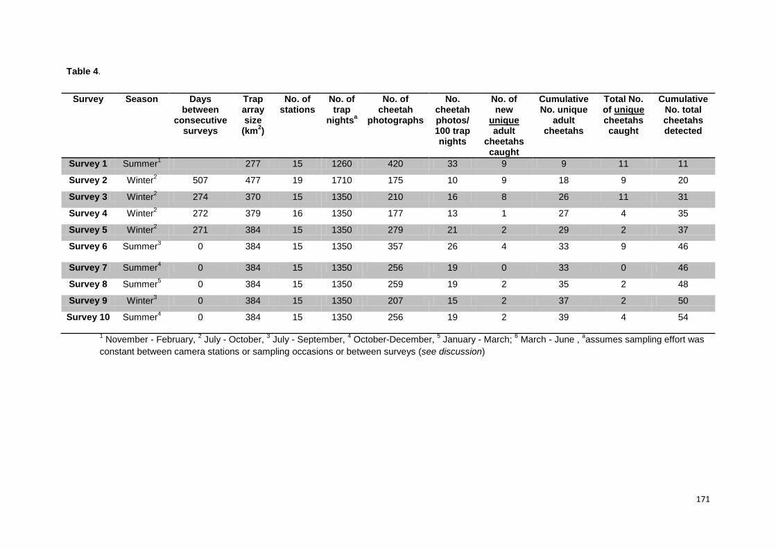
171
Table 4.
Survey Season Days between
consecutive surveys
Trap array size
(km2)
No. of stations
No. of trap
nightsa
No. of cheetah
photographs
No. cheetah photos/ 100 trap nights
No. of new
unique adult
cheetahs caught
Cumulative No. unique
adult cheetahs
Total No. of unique cheetahs caught
Cumulative No. total cheetahs detected
Survey 1 Summer1 277 15 1260 420 33 9 9 11 11
Survey 2 Winter2 507 477 19 1710 175 10 9 18 9 20
Survey 3 Winter2 274 370 15 1350 210 16 8 26 11 31
Survey 4 Winter2 272 379 16 1350 177 13 1 27 4 35
Survey 5 Winter2 271 384 15 1350 279 21 2 29 2 37
Survey 6 Summer3 0
384 15 1350 357 26 4 33 9 46
Survey 7 Summer4 0 384 15 1350 256 19 0 33 0 46
Survey 8 Summer5 0 384 15 1350 259 19 2 35 2 48
Survey 9 Winter3 0 384 15 1350 207 15 2 37 2 50
Survey 10 Summer4 0
384 15 1350 256 19 2 39 4 54
1 November - February,
2 July - October,
3 July - September,
4 October-December,
5 January - March;
6 March - June ,
aassumes sampling effort was
constant between camera stations or sampling occasions or between surveys (see discussion)
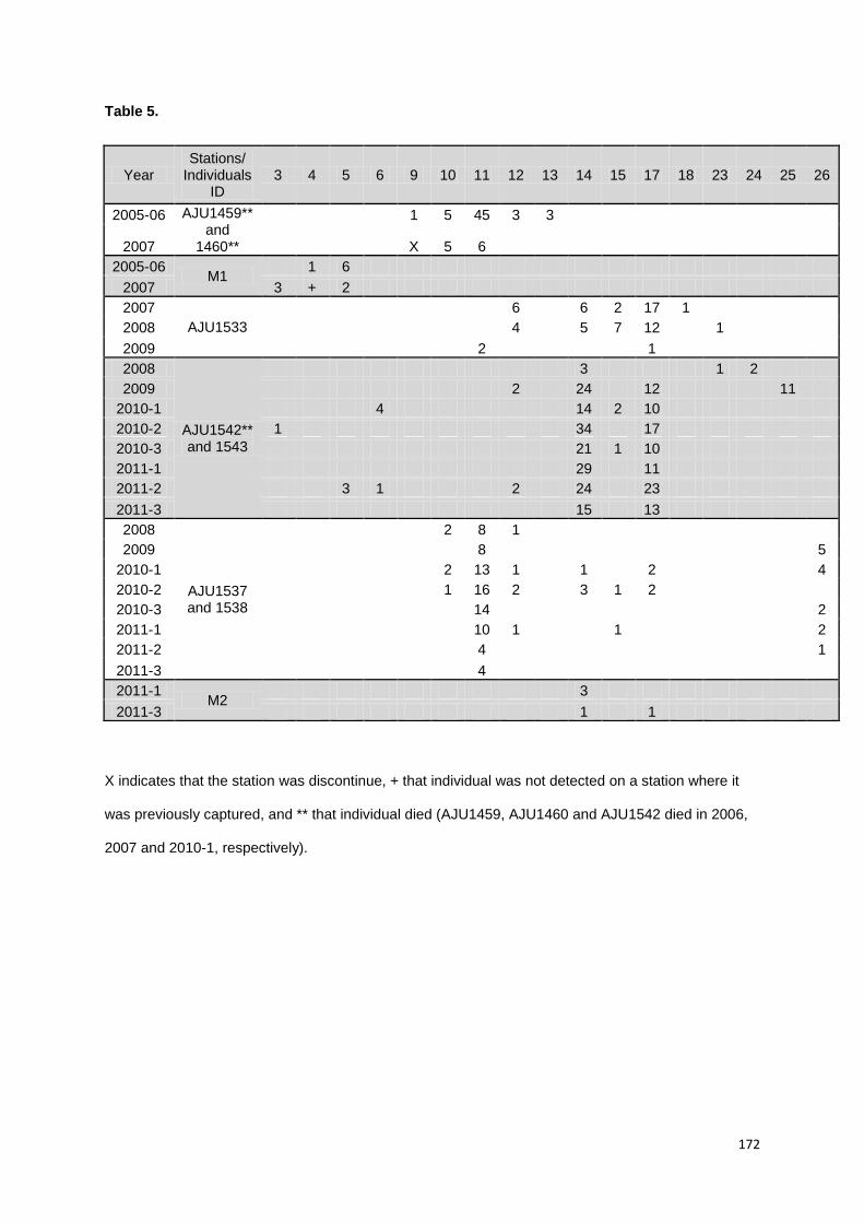
172
Table 5.
Year Stations/
Individuals ID
3 4 5 6 9 10 11 12 13 14 15 17 18 23 24 25 26
2005-06 AJU1459** and
1460**
1 5 45 3 3
2007 X 5 6
2005-06 M1
1 6
2007 3 + 2
2007
AJU1533
6 6 2 17 1
2008
4
5 7 12
1
2009 2 1
2008
AJU1542** and 1543
3 1 2
2009 2 24 12 11
2010-1 4 14 2 10
2010-2 1 34 17
2010-3 21 1 10
2011-1 29 11
2011-2 3 1 2 24 23
2011-3 15 13
2008
AJU1537 and 1538
2 8 1
2009
8
5
2010-1
2 13 1
1
2
4
2010-2
1 16 2
3 1 2
2010-3
14
2
2011-1
10 1
1
2
2011-2
4
1
2011-3 4
2011-1 M2
3
2011-3 1 1
X indicates that the station was discontinue, + that individual was not detected on a station where it
was previously captured, and ** that individual died (AJU1459, AJU1460 and AJU1542 died in 2006,
2007 and 2010-1, respectively).
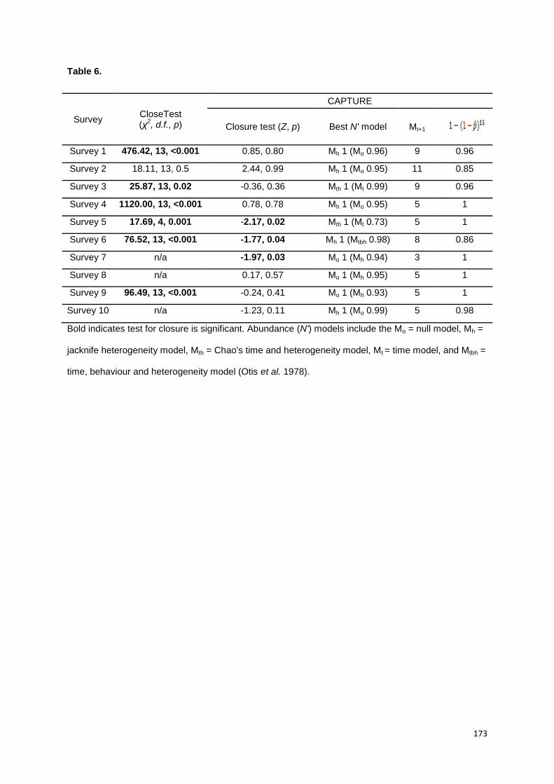
173
Table 6.
Survey CloseTest (χ
2, d.f., p)
CAPTURE
Closure test (Z, p) Best N' model Mt+1
Survey 1 476.42, 13, <0.001 0.85, 0.80 Mh 1 (Mo 0.96) 9 0.96
Survey 2 18.11, 13, 0.5 2.44, 0.99 Mh 1 (Mo 0.95) 11 0.85
Survey 3 25.87, 13, 0.02 -0.36, 0.36 Mth 1 (Mt 0.99) 9 0.96
Survey 4 1120.00, 13, <0.001 0.78, 0.78 Mh 1 (Mo 0.95) 5 1
Survey 5 17.69, 4, 0.001 -2.17, 0.02 Mth 1 (Mt 0.73) 5 1
Survey 6 76.52, 13, <0.001 -1.77, 0.04 Mh 1 (Mtbh 0.98) 8 0.86
Survey 7 n/a -1.97, 0.03 Mo 1 (Mh 0.94) 3 1
Survey 8 n/a 0.17, 0.57 Mo 1 (Mh 0.95) 5 1
Survey 9 96.49, 13, <0.001 -0.24, 0.41 Mo 1 (Mh 0.93) 5 1
Survey 10 n/a -1.23, 0.11 Mh 1 (Mo 0.99) 5 0.98
Bold indicates test for closure is significant. Abundance (N') models include the Mo = null model, Mh =
jacknife heterogeneity model, Mth = Chao's time and heterogeneity model, Mt = time model, and Mtbh =
time, behaviour and heterogeneity model (Otis et al. 1978).
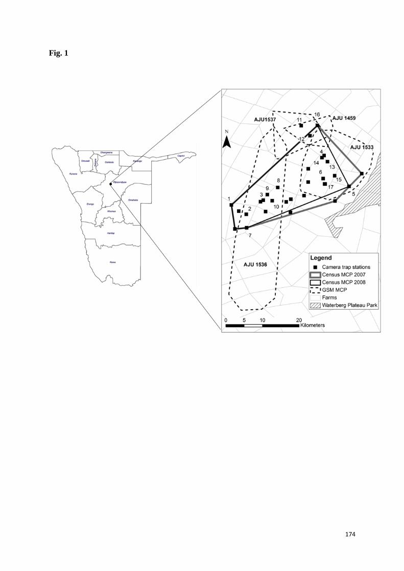
174
Fig. 1
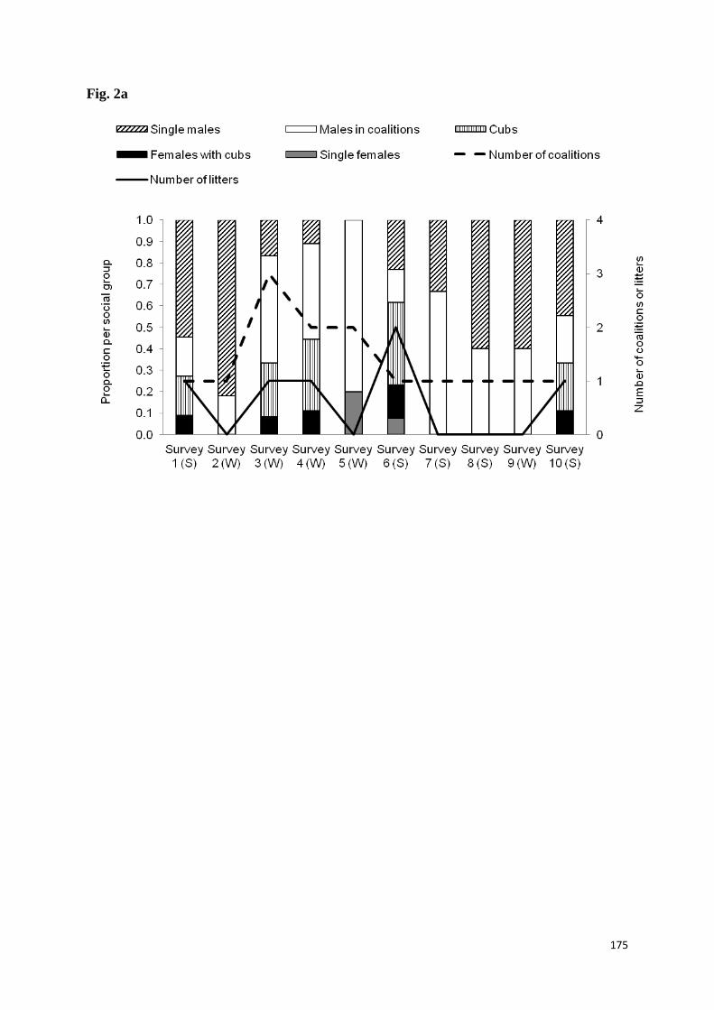
175
Fig. 2a
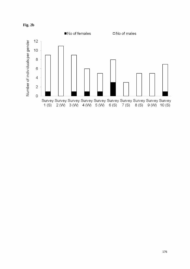
176
Fig. 2b
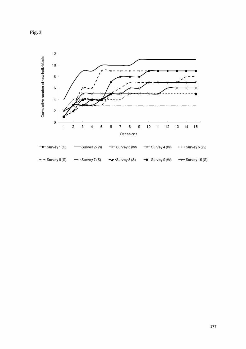
177
Fig. 3
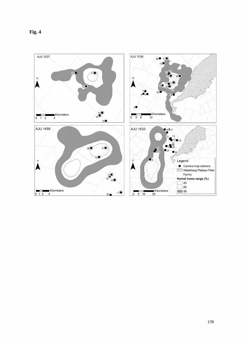
178
Fig. 4
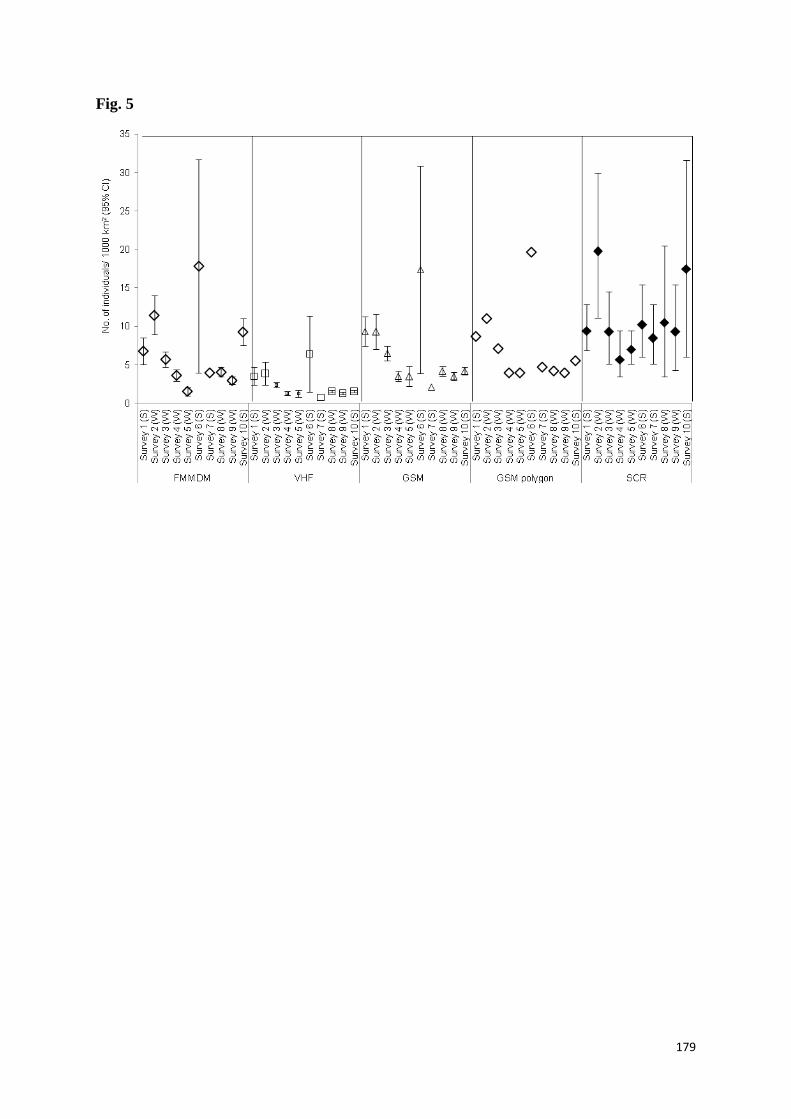
179
Fig. 5
180
SUPPLEMENATRY INFORMATION S1
Figure S1. Location of the study area in Namibia with annual trapping areas 2005 through
2011, with the minimum convex polygons of the four collared male cheetahs and the stations
where different cheetahs were detected during the study (labelled 1 through 17).
Figure S2 Estimates and posterior summary for cheetah capture probability, population size
estimate and activity centers, buffer width and range movement parameter, and density
estimates for the 10 three-month surveys (Namibia: 2005 - 2011). Precision for CAPTURE
and spatial capture recapture estimates are presented with 95% confidence intervals
determined using standard error and deviation, respectively. Estimates were considered to be
statistically significant at α = 0.05 if 95% high posterior distribution (HPD) or confidence
intervals (CI) did not overlap by more than half. (A) Capture probabilities derived using the
CAPTURE (p-hat) and SRC parameter that indicates the mean posterior distribution if the
camera trap is located an activity center (λ), which was converted into a capture probability
using 1-exp(-λ). (B) Capture probability prior and post initial encounter. (C) Abundance
estimates based on CAPTURE abundance best models (Mh, Mth or Mtbh, see Table 3) and
the SRC posterior estimate of N, the number of activity centers in region S. (D) PSI, the
probability of an individual in the augmented population being part of the sampled
population. (E) Buffer width estimates for the: Global System for Mobile (GSM), Very High
Frequency (VHF), full mean maximum distance moved (FMMDM), SRC animal movement
parameter which approximates a home range radius (s ~ HR) and actual SRC s posterior
mean. The solid line represents the average 95% GSM HR radius.
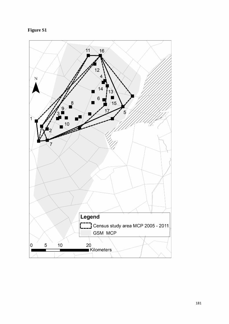
181
Figure S1
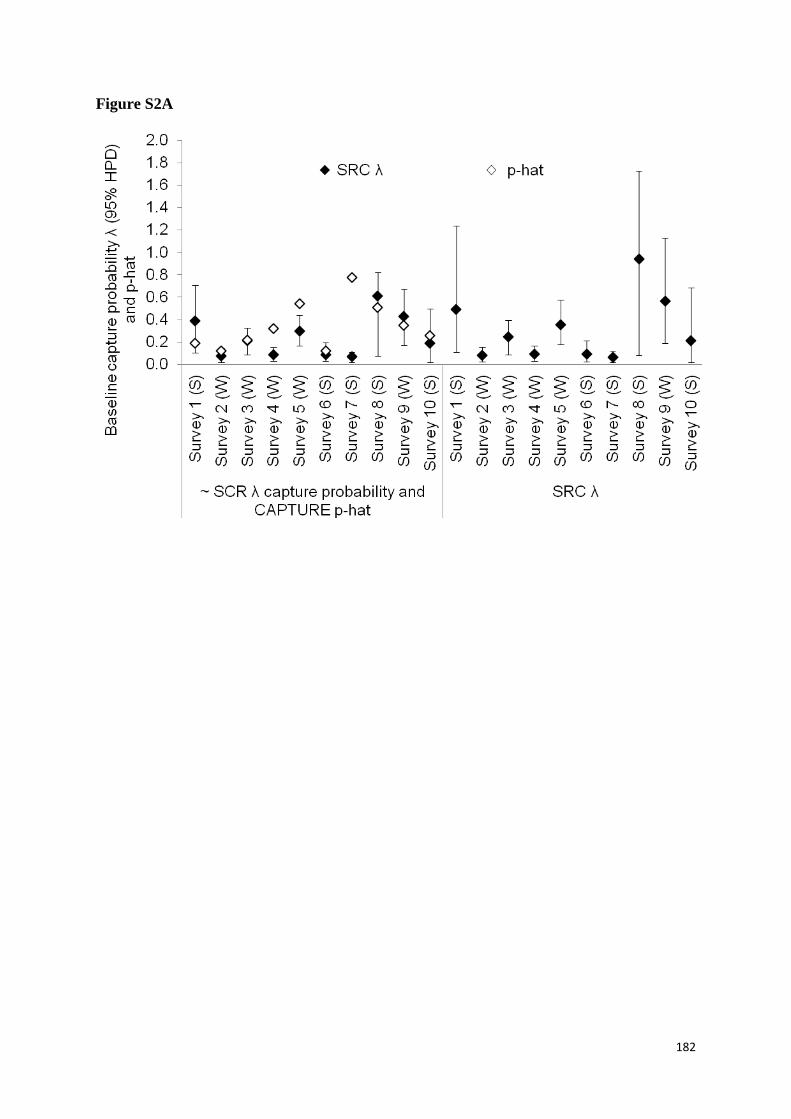
182
Figure S2A
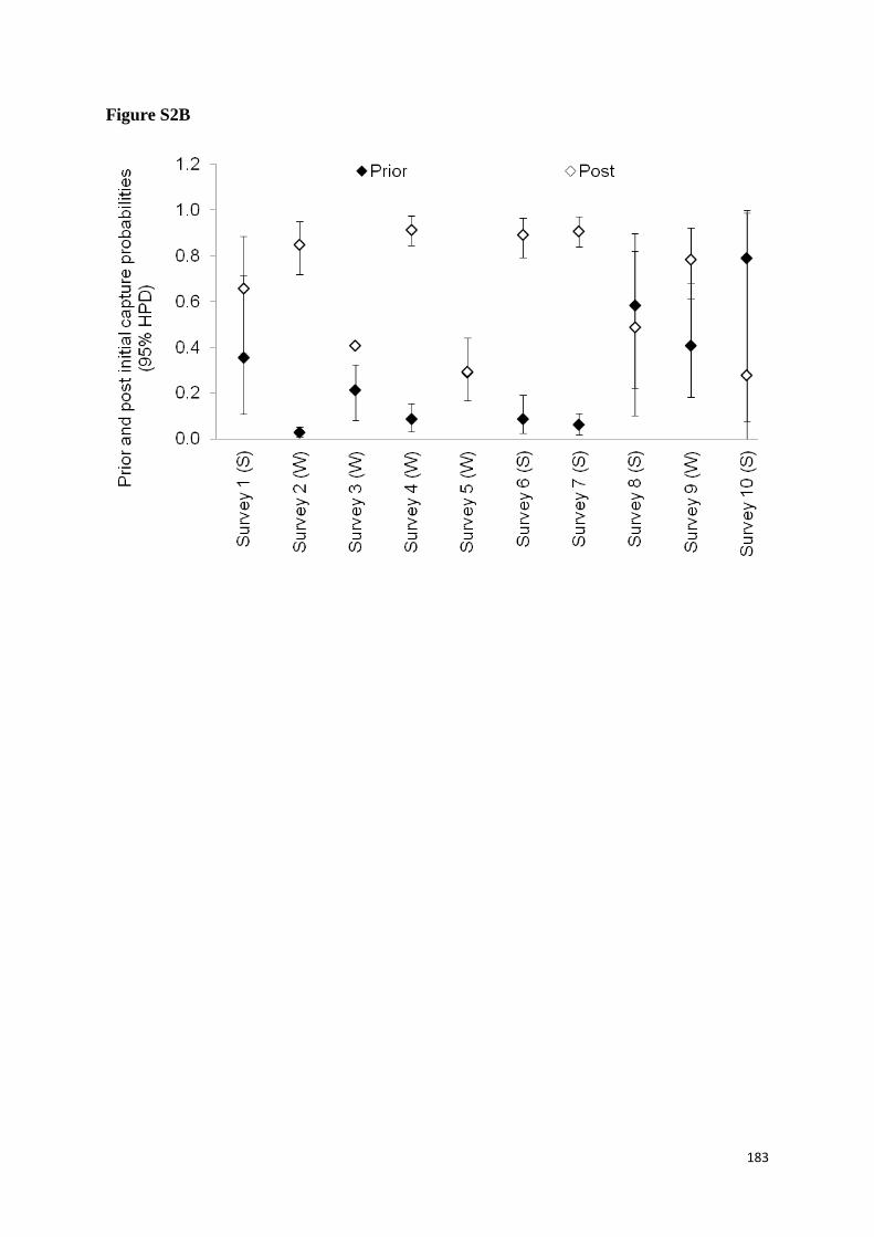
183
Figure S2B
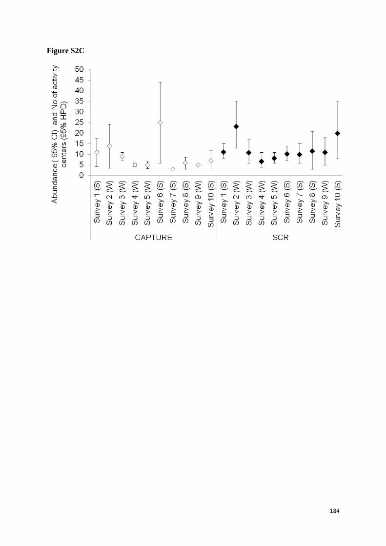
184
Figure S2C
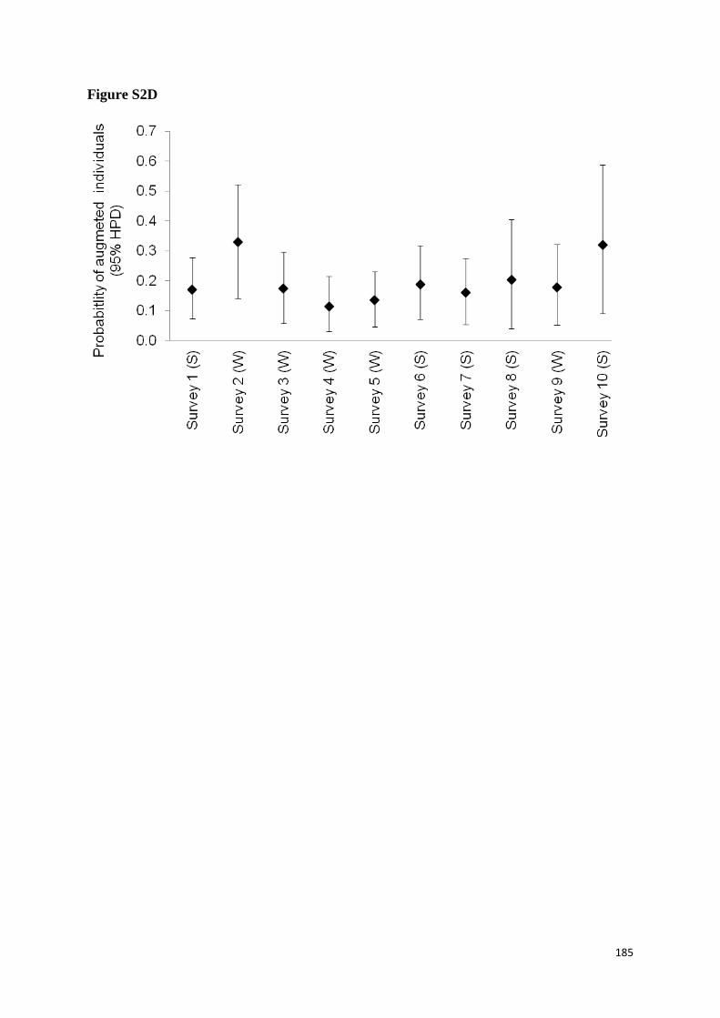
185
Figure S2D
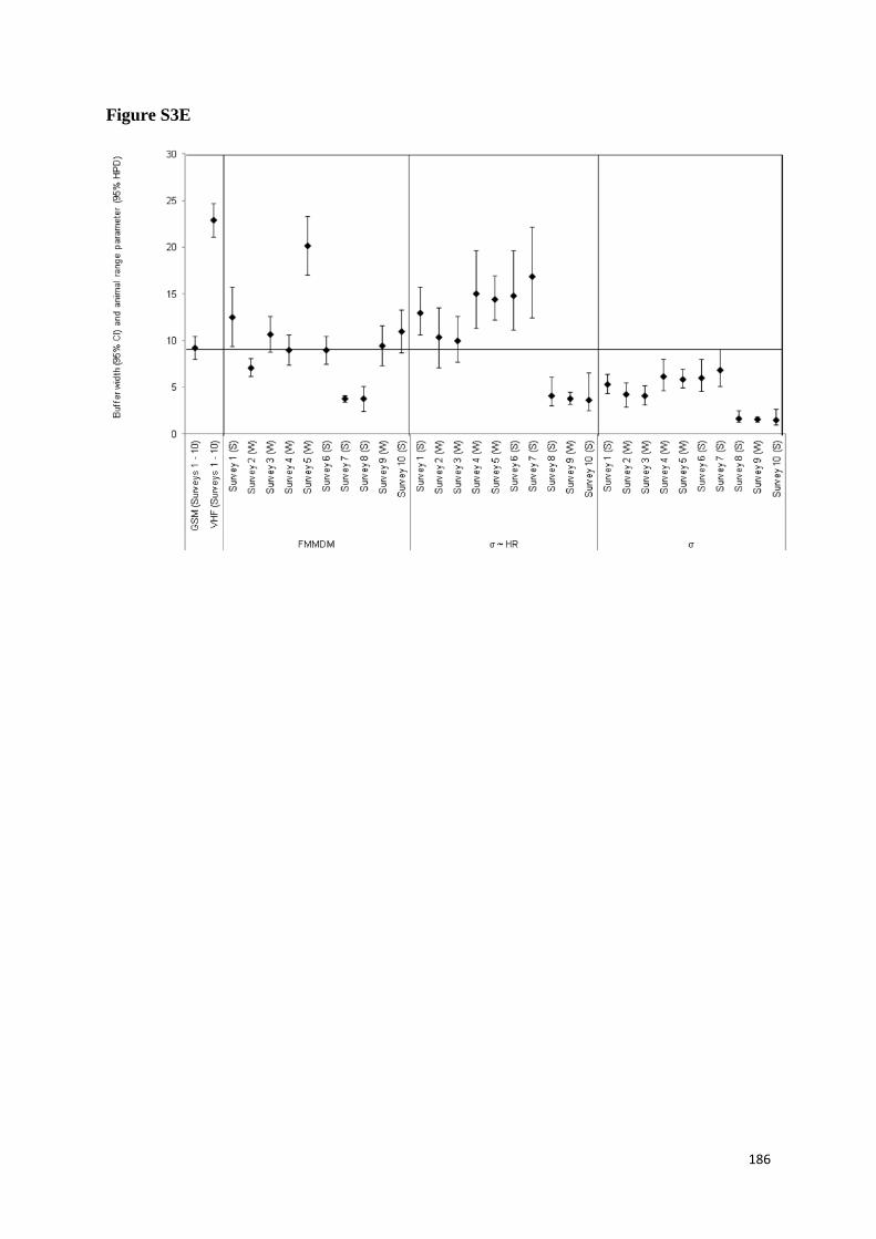
186
Figure S3E
187
Captions for Tables
Table S1 Cheetah density estimates per 1000 km2 in Namibia based non-spatial and
spatial methods (SRC). Non-spatial include estimating the effective sampled area by
buffering the camera trapping polygon with the full mean maximum distance moved
(FMMDM), the 95% home range radius from four radio collared cheetahs in this
study (GSM) and that from a previous study (VHF) as well as a minimum density
based on the 95% minimum convex polygon (GSM polygon).
Table S2 The 95% minimum convex polygon (MCP) and kernel home range
estimates of the four GSM collared with period tracked and GPS fixes.
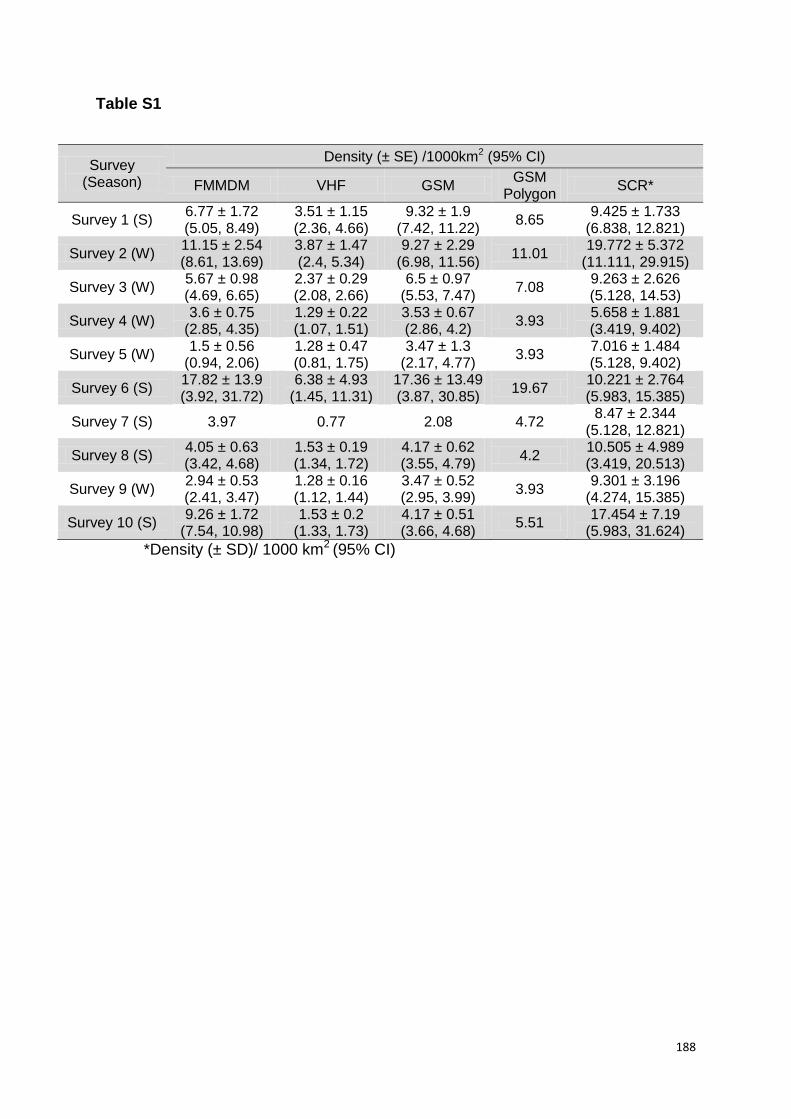
188
Table S1
Survey (Season)
Density (± SE) /1000km2 (95% CI)
FMMDM VHF GSM GSM
Polygon SCR*
Survey 1 (S) 6.77 ± 1.72 (5.05, 8.49)
3.51 ± 1.15 (2.36, 4.66)
9.32 ± 1.9 (7.42, 11.22)
8.65 9.425 ± 1.733
(6.838, 12.821)
Survey 2 (W) 11.15 ± 2.54 (8.61, 13.69)
3.87 ± 1.47 (2.4, 5.34)
9.27 ± 2.29 (6.98, 11.56)
11.01 19.772 ± 5.372
(11.111, 29.915)
Survey 3 (W) 5.67 ± 0.98 (4.69, 6.65)
2.37 ± 0.29 (2.08, 2.66)
6.5 ± 0.97 (5.53, 7.47)
7.08 9.263 ± 2.626 (5.128, 14.53)
Survey 4 (W) 3.6 ± 0.75
(2.85, 4.35) 1.29 ± 0.22 (1.07, 1.51)
3.53 ± 0.67 (2.86, 4.2)
3.93 5.658 ± 1.881 (3.419, 9.402)
Survey 5 (W) 1.5 ± 0.56
(0.94, 2.06) 1.28 ± 0.47 (0.81, 1.75)
3.47 ± 1.3 (2.17, 4.77)
3.93 7.016 ± 1.484 (5.128, 9.402)
Survey 6 (S) 17.82 ± 13.9 (3.92, 31.72)
6.38 ± 4.93 (1.45, 11.31)
17.36 ± 13.49 (3.87, 30.85)
19.67 10.221 ± 2.764 (5.983, 15.385)
Survey 7 (S) 3.97 0.77 2.08 4.72 8.47 ± 2.344
(5.128, 12.821)
Survey 8 (S) 4.05 ± 0.63 (3.42, 4.68)
1.53 ± 0.19 (1.34, 1.72)
4.17 ± 0.62 (3.55, 4.79)
4.2 10.505 ± 4.989 (3.419, 20.513)
Survey 9 (W) 2.94 ± 0.53 (2.41, 3.47)
1.28 ± 0.16 (1.12, 1.44)
3.47 ± 0.52 (2.95, 3.99)
3.93 9.301 ± 3.196
(4.274, 15.385)
Survey 10 (S) 9.26 ± 1.72
(7.54, 10.98) 1.53 ± 0.2
(1.33, 1.73) 4.17 ± 0.51 (3.66, 4.68)
5.51 17.454 ± 7.19
(5.983, 31.624)
*Density (± SD)/ 1000 km2 (95% CI)
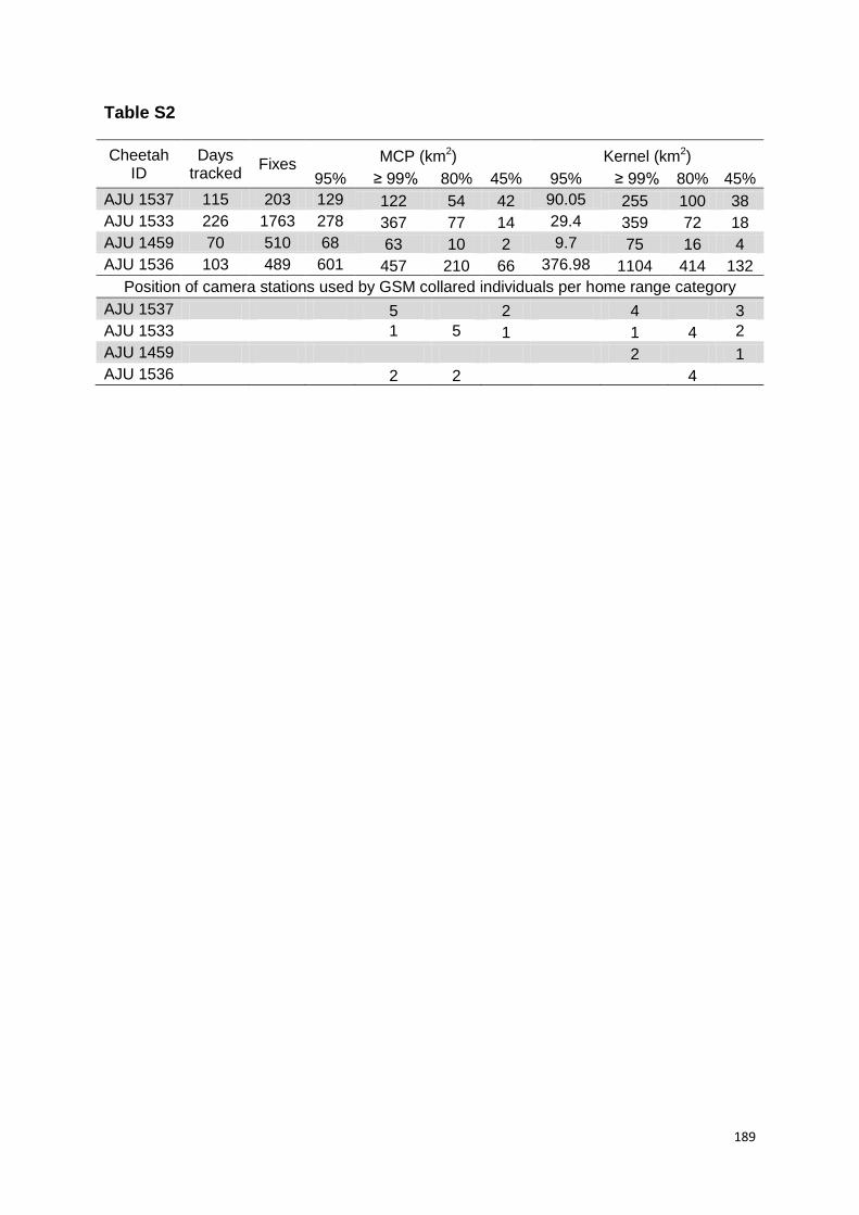
189
Table S2
Cheetah ID
Days tracked
Fixes MCP (km2) Kernel (km2)
95% ≥ 99% 80% 45% 95% ≥ 99% 80% 45%
AJU 1537 115 203 129 122 54 42 90.05 255 100 38
AJU 1533 226 1763 278 367 77 14 29.4 359 72 18
AJU 1459 70 510 68 63 10 2 9.7 75 16 4
AJU 1536 103 489 601 457 210 66 376.98 1104 414 132
Position of camera stations used by GSM collared individuals per home range category
AJU 1537 5 2 4 3
AJU 1533
1 5 1
1 4 2
AJU 1459 2 1
AJU 1536 2 2 4

190
Chapter V
191
Insights of temporal activity patterns of resident individual cheetahs, in north-
central Namibia
Author list:
Ezequiel Chimbioputo Fabiano 1, 2
Matti Nghikembua 2
Eduardo Eizirik 1
Laurie Marker 2
Affiliations:
1. Laboratório de Biologia Genômica e Molecular, Faculdade de Biociências,
Pontifícia Universidade Católica do Rio Grande do Sul, Porto Alegre, RS 90619-900,
Brazil
2. Cheetah Conservation Fund, PO Box 1755, Otjiwarongo, Namibia. Fax: 264 67
306247
Email addresses:
192
Corresponding authors:
Ezequiel C. Fabiano
Cheetah Conservation Fund,
P.O. Box 1755, Otjiwarongo, Namibia.
Fax: 264 67 306247
Author Contributions: ECF conceived, designed, performed data analyses, and wrote
the manuscript; EE, LM and MN provided editorial advice.
193
Abstract
The activity patterns of cheetahs are largely unknown for populations where it
coexists only with part of the large carnivore guilds. This is the case for the Namibian
cheetah population residing on farmlands, where dominant predators, lions and
spotted hyenas, are absent, but leopards and brown hyenas persist. In this study, we
used photographic captures of 10 three months surveys conducted between 2005
and 2011 (five in winter and summer), to describe the temporal activity patterns of
cheetahs across seasons at least to scent marking sites. This is the first insight into
inter-individual interactions. A strong nocturnal and crepuscular activity pattern was
retrieved which was consistent across seasons essentially for males as females had
a low sample size. At the individual level, activities patterns between a resident
single male and a coalition of two male, overlapped but differed in the time of activity
peak, with the latter increasing in activity at times when the former declines. This
suggests that movements by males and at least in respect towards scent marking
sites occurs during nighttime. Ultimately, these findings contribute to the growing
evidence of cheetahs being nocturnal across its range.
194
Introduction
Activity patterns represent periods of time when living organisms engage on different
daily functions aimed at meeting their biological needs but fine-tuned to allow for
flexible responses (Halle 2000). Different forms on temporal niche include diurnality
(e.g. Andean cats Leopardus jacobita [Lucherini et al. 2009]), nocturnality (e.g. lions
Panthera leo [Hayward and Slotow 2009]), crepuscularity (e.g. tiger Cryptoprocta
ferox [Gerber et al. 2012]) or a combination of these as well as cathermal (e.g.
leopards P. pardus) (see Hayward and Slotow 2009 for a meta-analysis on African
large carnivores). Linkie and Ridout (2011) found tiger Panthera tigris crepuscular
behaviour to overlap with that of its prey. This diversity within the temporal dimension
alongside the spatial and food dimensions of the ecological niche provides a
framework for understanding resource partitioning among sympatric species and
individuals within a population (Schoener 1974).
The cheetah alongside wild dogs and brown hyena are sub-dominant to lions
and spotted hyenas that exert an influence on the ecology of the formers (Mills
2005). In the Serengeti, cheetahs configure their spatial distribution as to minimize
intraspecific competition with dominant large predators (Durant 2000). In turn,
findings are less consistent regarding activity patterns. For example, based on
observations (movements, kills) when coexisting with dominant predators cheetahs
tend to exhibit a diurnal crepuscular behaviour (Durant 1998; Bothma and Walker
1999) with a daily peak activity occurring in late evening/afternoon (Hayward and
Slotow 2009). This pattern was attributed to top-down effects (Hayward and Slotow
2009). In turn, in the Sahara Mountains, cheetahs increase activity during the cooler
time of the day (nighttime) (Bothma and Walker 1999) as it is the case of cheetahs in
195
the Okavango Delta (Cozzi et al. 2012). Cozi et al. (2012) also indicates cheetah
activity to be influence by lunar cycles.
In Namibia, limited observations also indicate a nocturnal cheetah activity
pattern (McVittie 1979; Marker et al. 2008a). However, the temporal activity patterns
at the inter- or intra-sexual levels, remains largely unknown. Furthermore, cheetahs
in Namibia farmlands only coexist with leopards and brown hyenas, as dominant
predators are absent (Marker-Kraus et al. 1996). These ecological setting differs
from that of most antecedent studies (e.g. Durant 2000; Hayward and Slotow 2009;
Cozzi et al. 2012). This nocturnal activity pattern is considered to be a behavioural
response to competitor release (McVittie 1979) or to minimize overlap with human
activities (Hayward and Slotow 2009) and need to extend their temporal niche to
meet their biological needs (starvation driven) (Cozzi et al. 2012). At the individual
level, heterogeneity is has been linked to ecological factors such as patrolling
territories boundaries by males at night (Grünewalder et al. 2012). Altogether,
intraguild relationships are variable and influenced by ecological conditions (Hallew
2000; Mills 2005). To ascertain that this nocturnal pattern is ubiquitous additional
studies are required, under similar or different ecological settings, which is the aim of
this study.
Here, we provide insights on the temporal activity patterns of a cheetah
population that coexist with an imcomplete large carnivore guild based on a six years
remote camera trap dataset, 10 surveys five per summer and winter, respectivley.
Specific objectives were (1) to quantify activity patterns per season, (2) compare
activity patterns between seasons and (3) provide insights into inter-individual
temporal activity patterns. While the study extends and complements antecedent
studies (e.g. Durant 2000; Marker et al. 2008a; Hayward and Slotow 2009; Cozzi et
196
al. 2012) it differs in a number of aspects including methodology, sample size,
sampling duration, and ecological setting, but mostly by basing activity patterns on
photo captures of individuals at scent marking posts. Understanding activity patterns
in Namibia is of significance as it provides information regarding the species
ecological niche information that can aid when devising conservation measures
related to depredation.
Methods
STUDY DESIGN AND DATA COLLECTION
To assess species and individual cheetah temporal activity patterns, we used a
remote camera trap (RCT) dataset of a 10 three months cheetah surveys conducted
in north-central Namibia. The study area and design are fully described in Chapter IV
(but also Marker et al. [2008a, b]). However, we provide a description of the study
design that is of relevance for exploring activity patterns.
RCT surveys were conducted annually for three months from 2005 to 2009,
and then continuously between July 2010 and December 2011, encompassing an
average area of 377 km2 (SD + 41.15 km2) (Fig. 1). To be consistent with our
previous work (Marker, Fabiano and Nghikembua 2008), we stratified the continuous
effort (i.e. 2010 through 2011 data set) into six surveys, of 90 days each. Although
Namibia is considered to have three seasons, for the purpose of this study, surveys
were grouped into two main seasons, Summer (Nov – May) and Winter (June – Oct).
Overall, five surveys each were conducted during the summer and winter seasons.
During the course of the study, 32 different sampling stations were deployed (15 to
19 per annum). Sixty-three percent (n = 20) of the stations were located at scent
marking posts and 19% (n = 6) either next to roads/fence lines and in close proximity
197
to cheetah captive facilities. Inter-camera distances were on average 17 km (± 9.24
km). We used DeerCamTM DC200 (DeerCam, Park Falls, WI, USA) and Bushnell
Trophy (Trophy Cam 2009, Kansas, USA) cameras from 2005 to 2009 and 2010
through to 2011, respectively. In 2008, one station had a Moultrie M60 digital camera
(Georgia, USA). We placed two cameras per station, mounted ca. 75 cm above the
ground and 5 m apart. We checked camera sites every 2 to 5 days to ensure
functionality, change film/memory card and/or batteries. For data management,
pictures from developed films were logged into an Excel database, while CamTrap
software (Harris et al. 2010) was used for memory cards.
Cheetahs individuals were identified manually based on unique spot patterns,
which remain unaltered throughout their lifetime (Caro and Durant 1991). Gender
was determined using cues such as the presence of visible genitals, ear tag position
for individuals previously physically handled by CFF (i.e. right for males and left for
females) or accompanying cubs. A cheetah was classified as either a cub (≤ 1 years
old) or adult (> 1 year old); male or female; or as single, member of male coalition or
breeding female (i.e. with accompanying cubs). We also classified individuals as
resident if they were captured during at least two consecutive inter-annual surveys
(i.e. the six surveys spaced equally apart) or during two consecutive stratified
surveys within the 2010 - 2011 continuous survey (Caro and Collins 1987; Barlow et
al. 2009). All other individuals were treated as non-resident. Likewise, we considered
a site an integral component of an individual’s HR if it was visited continuously on all
surveys in which the individual was detected. This consideration was limited to
residents.
TEMPORAL AND SPATIAL UTILISATION PATTERNS OF CHEETAHS BASED ON
RCT DATA
198
Temporal patterns for all detected cheetahs were determined as the
percentage of photos taken per hour in a 24-hour cycle using time and date tags on
photographs. Only photos taken more than a minute apart were included. While we
recognize that this approach provides only preliminary findings as a one-minute
difference between consecutives photos may introduce autocorrelation, this may not
constitute a major concern when exploring activity patterns (Jim Anderson pers.
comm.). The Kuiper's test was applied to test whether the distribution of photos
throughout the day was uniform per season as implemented in the Circular R
package (Agostinelli and Lund 2012). Furthermore, we subdivided the data into
dawn (04:00 - 07:59), day (08:00 - 15:59), dusk (16:00 - 19:59) and night (20:00 -
03:59), and assessed for differences in proportion of visitation among these periods
using a likelihood-ratio chi-square test in a contingency table (after Gerber et al.
2012). Duration of diel periods followed mainly Haywared and Slotow (2009).
Conditioned on significance a partial chi-square was used to assess significant
contribution of each diel period. Activity peaks were determined as hours with the
highest proportion of photographs. In addition to activity patterns at population level,
we also assessed interspecific overlap.
Results
TEMPORAL AND SPATIAL UTILISATION PATTERNS OF CHEETAHS BASED ON
RCT DATA
The temporal activity patterns of resident cheetahs are presented in Fig. 2. Based on
a total 1813 photos taken, 13%, 16%, 42% and 30% were at daylight, dusk,
nocturnal and dawn (Fig. 2A). Hence, 46%, 42% and only 16% of the photos were
taken during crepuscular, nocturnal and daylight periods, respectively. When
199
considering across seasons even though fewer pictures were obtained in summer
than in winter this difference was insignificant (n = 849 and 970, respectively; U =
0.293, P > 0.05). However, activity patterns were the same across seasons with
cheetahs showing predominantly a nocturnal and crepuscular pattern (χ2 = 12.26,
d.f. = 3, P > 0.05) (Fig. 2B, C). We noticed an opposite trend in the number of photos
taken between 03:00 and 07:00, with an increase in winter and reduction in summer
(Fig. 2D). Kuiper's test provided evidence that this distribution pattern of photos
throughout the day (08:00 - 16:00) was nearly significant in summer (K = 1.75, 0.05
< P < 0.10).
The few recaptures by non-residents limits the identification of temporal
overlap at individual level (Fig S1). However, restricted to resident individuals there
appears to be a certain degree of temporal overlap with differences in the time of
peaks (Fig. S1A, D, F, G). For example, resident individual M13 shows a decline in
the number of photos between mid-night and 08:00 (Fig S1G). Conversely, M17 and
M18 two peaks only occurred at 08:00 (overlapping with that of M13) and at dusk (~
18:00 - 19:00), an hour later than M13 peak.
Discussion
Cheetahs were found to exhibit a predominant nocturnal and crepuscular activity
patterns throughout the year, a finding that corroborates previous studies (McVittie
1979; Bissett and Bernard 2006; Marnewick et al. 2008; Cozzi et al. 2012).
Supporting evidence for this is the significant proportion of detections at camera sites
during crepuscular and nighttime across surveys and seasons (Fig. 2). Peaks of
activities across season were largely between 16:00 to 20:00, 20:00 to 00:00 and
200
00:00 to 08:00. This peak of activity in the late afternoon is similar to that of other
studies (e.g. 18:00 - 21:00, 16:00 - 17:00) (Hayward and Slotow 2009). Hence, the
crepuscular activity highlights the importance of this period possible for hunting while
avoidance during hot periods for physiological reasons. However, our findings run
counter the notion of cheetahs being predominantly diurnal.
Due to the biased male sex ratio, this activity pattern may pertain only to
males and at least with respect to scent marking sites. This would imply that
retrieved activity patterns might not to be representative of overall activity patterns of
cheetahs (i.e. detected, undetected, females). However, the timing of the few photos
for females were consistent with this pattern. Specifically these occured early
morning (05:00 - 09:00, n = 7) but also once at 10:00 and twice in the early evening
(19:00) (Fig. S1). Bissett and Bernard (2006) noted a similar pattern whereby the
activity pattern of a cheetah male coalition but not of females overlapped with that of
lions. Additionally, photos from RCT placed at waterholes indicate that visitation to
waterholes also follow a nocturnal crepescular pattern (out of 156 only one photo
was at between 08:00 and 16:00, unpublished data). Speed of four GSM collared
males cheetah also indicated nearly no movement during daytime. Altogether, this
indicates that cheetahs exhibit a nocturnal crepuscular pattern. Future studies with
larger datasets should explore this further.
The strictly nocturnal pattern runs counter previous studies (but see Cozzi et
al. 2012 for a similar conclusion). Discrepancies of conclusions could be due to
ecological settings of the different studies. Unlike is the case in our study area, other
studies were mosly based on data from protected areas where intraspecific
competition is intense due to the presence of dominant predators such as lions and
spotted hyenas (Eaton 1970; Durant 2000; Hayward and Slotow 2009). Hence, this
201
activity pattern could be due to competitor release. Nevertheless, limited evidence is
found on the literature supporting this hypothesis as it draws mostly on the
observation of dominant competitors (lions, leopards, spotted and brown hyenas)
being nocturnal (Hawyard and Slotow 2009). Furthermore, a recent study from a
study area where cheetahs coexist with its main predators also retrieved a nocturnal
(Cozzi et al. 2012). Their study also indicated that lunar cycles influence cheetah
activity pattern and that this behaviour allows cheetahs to maximize hunting
opportunities, thus the "starvation driven" hypothesis. Our study extends this
conclusion, to include ecological activities related to scent marking as being mostly
nocturnal. Cheetah photo-captures at waterholes also indicate nocturnal activity
(unpublished data). These studies re-iterate that large carnivore nocturnal traits are
deep embedded phylogenetically (Holt 2009) a case similar to rodents (Roll et al.
2006).
Alternatives hypothesis that could explain this activity pattern include
behavioural responses to adaptation to local prey species or human activity patterns
(foragining hypothesis) (Hayward and Slotow 2009). The foraging success
hypothesis postulates that predators tend to be more active at times that coincide
with their prey activity patterns (Hayward and Slotow 2009). Our data supports this
hypothesis, as cheetahs activity pattern overlapped largely with that of its prey (e.g.,
oryx, kudu, eland, red hartebeest, warthog) based on photo-captures at cheetah
scent-marking sites (Fig S2). Nevertheless, it also overlapped with that of other
carnivores such as leopard and jackals (Fig S2). This overlap may be facilitated by
the poor detection of cheetah scent by prey species and other carnivores due to the
negligible amount of sulphur on cheetah urine that makes their scent odourless
(unnoticeable) (Burger et al. 2006; Apps et al. 2012). Future studies, should explore
202
the relation between lunar cycle and species activity patterns (as per Cozzi et al.
2012).
Lastly, this shift could be an adaptation to minimize overlap with human
activity patterns. Such adjustments has been reported for other species such as lions
in the Makgadikgadi Pans National Park, Botswana (Valeix et al. 2012) or tigers in
the Chitwan National Park in Nepal (Carter et al. 2012) areas also characterized by
human wildlife conflict. Brown bears (Ursus arctos) also adjust on a seasonal and
daily basis to human activities (Ordiz et al. 2011). However, the low human density
and distribution in Namibia renders direct levels of disturbance to be the unlikely sole
cause of this shift as appears to be the case for tigers (Carter et al. 2012; Athreya et
al. 2013). Nevertheless, further understanding of the role of anthropogenic factors as
a causative factor requires a comparative study within protected areas Namibia (e.g.
adjacent Waterberg Plateau). Overall, we argue that this temporal activity pattern is
likely to be the result of interactions between carnivore guild composition, cheetah
social structure, prey availability, human-induced factors underlined by evolutionary
plasticity.
The differences in peak of activity among the different resident social groups,
single versus male coalitions, with the latter exhibiting fewer captures than the
former, suggests a possible role of social group on activity patterns. Eaton (1970)
hypothesized that scent marking on cheetah served as a "time-plan", aimed at
minimizing encounter rates among conspecifics. While differences on peak periods
at individual level partly support this hypothesis, in our study, this is counfounded by
the resident individuals' spatial organization. In other words, this temporal overlap
was due to the simultaneous temporal utilization of different scent marking sites by
203
resident individuals. We recommend future to explore further this aspect of temporal
segregation based on a larger sample.
Overall, this study shows that the temporal activity pattern of cheetahs in
north-central Namibia where it coexist with other large sympatric carnivores (leopard
and brown hyena) to be largely nocturnal and crepuscular. Coexistence with
conspecifics seems facilitated by temporal and spatial segregation, suggesting that
scent marking may play a significant role in minimizing potential direct contact, the
"time-plan" hypothesis of Eaton's (1970). The similarity in visitation rate to scent
marking sites highlights the significance of these sites possible for resource defence
or home range. Furthermore, the nocturnal activity part observed may exemplify
niche conservatism (Holt 2009). The findings invoke the inclusion of temporal activity
patterns in the conservation efforts essentially when devising human-wildlife conflict
mitigation. We recommend future studies to explore simultaneously the spatial
temporal activity patterns of sympatric predators and their prey, within and outside
protected areas in Namibia.
Acknowledgements
We would like to thank the Cheetah Conservation Fund (CCF) staff members, in
particularly Carolyn Whitesell, Katherine Forsythe, Marjolein van Dieren, Suzie
Kenny and CCF interns and volunteers, particularly Earthwatch who, through the
years assisted with data collection and processing. We are grateful to the Ministry of
Environment and Tourism for granting a research permit. Funding for this research is
thanks to Cheetah Conservation Fund, EarthWatch, Columbus Zoo and CAPES.
References
204
Agostinelli C, Lund U (2012) R package “circular”: Circular Statistics (version 0.4-3)
Apps P, Mmualefe L, McNutt JW (2012) Identification of volatiles from the secretions
and excretions of African wild dogs (Lycaon pictus). J. Chem. Ecol. 38:1450–61.
doi:10.1007/s10886-012-0206-7
Athreya V, Odden M, Linnell JDC, Krishnaswamy J, Karanth U (2013) Big Cats in
Our Backyards: Persistence of Large Carnivores in a Human Dominated
Landscape in India. PLoS ONE 8: e57872. doi:10.1371/journal.pone.0057872
Barlow ACD, Mcdougal C, Smith JLD, Gurung B, Bhatta SR, Kumal S, Mahato B,
Tamang DB (2009) Temporal Variation in Tiger (Panthera tigris) Populations
and Its Implications for Monitoring. J Mammal 90:472–478
Bothma J du P, Walker C (1999) Larger carnivores of the African savannas.
Springer, New York, USA
Bissett C, Bernard RTF (2006) Habitat selection and feeding ecology of the cheetah
(Acinonyx jubatus) in thicket vegetation: is the cheetah a savanna specialist? J
Zool 271:310 -317
Caro TM, Collins DA (1987) Male Cheetah Social Organization and Territoriality.
Ethology 74:52-64
Caro TM, Durant SM (1991) Use of Quantitative Analyses of Pelage Characteristics
to Reveal Family Resemblances in Genetically Monomorphic Cheetahs.J Hered
82:8–14
205
Carter NH, Shrestha BK, Karki JB, Pradhan NMB, Liu J (2012) Coexistence between
wildlife and humans at fine spatial scales. PNAS 109:15360–5
doi:10.1073/pnas.1210490109
Cozzi G, Broekhuis F, McNutt JW, Turnbull L, Macdonald D, Schimid B (2012) Fear
of the dark or dinner by moonlight ? Reduced temporal partitioning among
Africa’s large carnivores. Ecology 93: 2590–2599
Durant SM (2000) Living with the enemy: avoidance of hyenas and lions by cheetahs
in the Serengeti. Behav Ecol 11:624–632. doi:10.1093/beheco/11.6.624
Eaton R (1970) Group interactions, spacing and territoriality in cheetahs. Z
Tierpsychol 27:481–91.
Gerber BD, Karpanty SM, Randrianantenaina J (2012) Activity patterns of carnivores
in the rain forests of Madagascar: implications for species coexistence. J
Mammal 93:667–676 doi:10.1644/11-MAMM-A-265.1
Grünewälder S, Broekhuis F, Macdonald DW, Wilson AM, McNutt JW, Shawe-Taylor
J, Hailes S (2012) Movement activity based classification of animal behaviour
with an application to data from cheetah (Acinonyx jubatus). PLOS ONE 7:
e49120 doi:10.1371/journal.pone.0049120
Halle S (2000) Ecological relevance of daily activity patterns. In Halle S, Stenseth
NC (eds) Activity Patterns in Small Mammals – an Ecological Approach.
Springer, Berlin, pp 67–90
Harris G, Thompson R, Childs LJ, Sanderson GJ (2010) Automatic Storage and
analysis of camera trap data. Bull Ecol Soc Am 91:352 – 360
206
Hayward MW, Hayward GJ (2006) Activity patterns of reintroduced lion Panthera leo
and spotted hyaena Crocuta crocuta in the Addo Elephant National Park , South
Africa. Afr J Ecol 45:135–141
Hayward MW, Slotow R (2009) Temporal partitioning of activity in large African
carnivores : tests of multiple hypotheses. S Afr J Wildl Res 39:109–125
Holt RD (2009) Bringing the Hutchinsonian niche into the 21st century: ecological
and evolutionary perspectives. PNAS 106 Suppl 19659–65.
doi:10.1073/pnas.0905137106
Kelly MJ, Laurenson MK, Fitzgibbon CD, Collins DA, Durant SM, Frame W, Bertram
BCR, Caro TM (1998) Demography of the Serengeti cheetah (Acinonyx jubatus)
population : the first 25 years. J Zool 244: 473 – 488
Linkie M, Ridout MS (2011) Assessing tiger-prey interactions in Sumatran
rainforests. J Zool 284:224–229
Lucherini M, Reppucci JI, Walker RS, Villalba ML, Wurstten A, Gallardo G, Iriarte A,
Villalobos R, Perovic P (2009) Activity Pattern Segregation of Carnivores in the
High Andes. J Mammal:1404–1409
Marker-Kraus L,Kraus D, Barnett D, Hurlburt S (1996) Cheetah survival on Namibian
farmlands. Cheetah Conservation Fund, Otjiwarango, Namibia
Marker L, Fabiano E, Nghikembua M (2008) The Use of Remote Camera Traps to
Estimate Density of Free- ranging Cheetahs in North-Central Namibia. Cat
News 1 22–24
207
Marker LL, Dickman AJ, Mills MGL, Jeo RM, Macdonald DW (2008) Spatial ecology
of cheetahs on north-central Namibian farmlands. J Zool 274 226–238
Marnewick K, Funston PJ, Karanth KU (2008) Evaluating camera trapping as a
method for estimating cheetah abundance in ranching areas. S Afr J Wildl Res
38:59–65
Mills MGL (2005) Large carnivores and biodiversity in African savanna ecosystems.
In: Ray JC, Redford KH, Steneck RS, Berger J (eds) Large Carnivores and the
Conservation of Biodiversity. Island Press, Washington, USA, pp 208-229
McVittie R (1979) Changes in the social behaviour of South West African cheetahs.
Madoqua 11: 191–84
Ordiz A, Støen O-G, Delibes M, Swenson JE (2011) Predators or prey? Spatio-
temporal discrimination of human-derived risk by brown bears. Oecologia
166:59–67 doi:10.1007/s00442-011-1920-5
Roll U, Dayan T, Kronfeld-Schor N (2006) Signals of profitability? Food colour
preferences in migrating juvenile blackcaps differ for fruits and insects. Evo Ecol
20: 479–490 doi:10.1007/s10682-006-0015-y
Schoener T (1974) Resource partitioning in ecological communities. Science
185:27–39 doi:10.1126/science.185.4145.27
Valeix, M., Hemson, G., Loveridge, A. J., Mills, G., & Macdonald, D. W. (2012).
Behavioural adjustments of a large carnivore to access secondary prey in a
208
human-dominated landscape. J Appl Ecol 49: 73–81 doi:10.1111/j.1365-
2664.2011.02099.x
Figure legends:
Fig. 1. Location of the study area in Namibia with annual trapping areas for 2007 and
2008, the home ranges of four collared male cheetahs (95% minimum convex
polygons; labelled as GSM MCP) and the camera trap stations where all cheetahs (n
= 54) were detected during the study (labelled 1 through 17). Collared males are
identified by AJU (Acinonyx jubatus ID#).
Fig. 2 Number of cheetah photographs per diel period per season (A), trends in the
number of photos per hour for the 5 winter (B) and 5 summer surveys (C) and overall
across seasons (D). Surveys were conducted between 2005 - 2011.
209
210
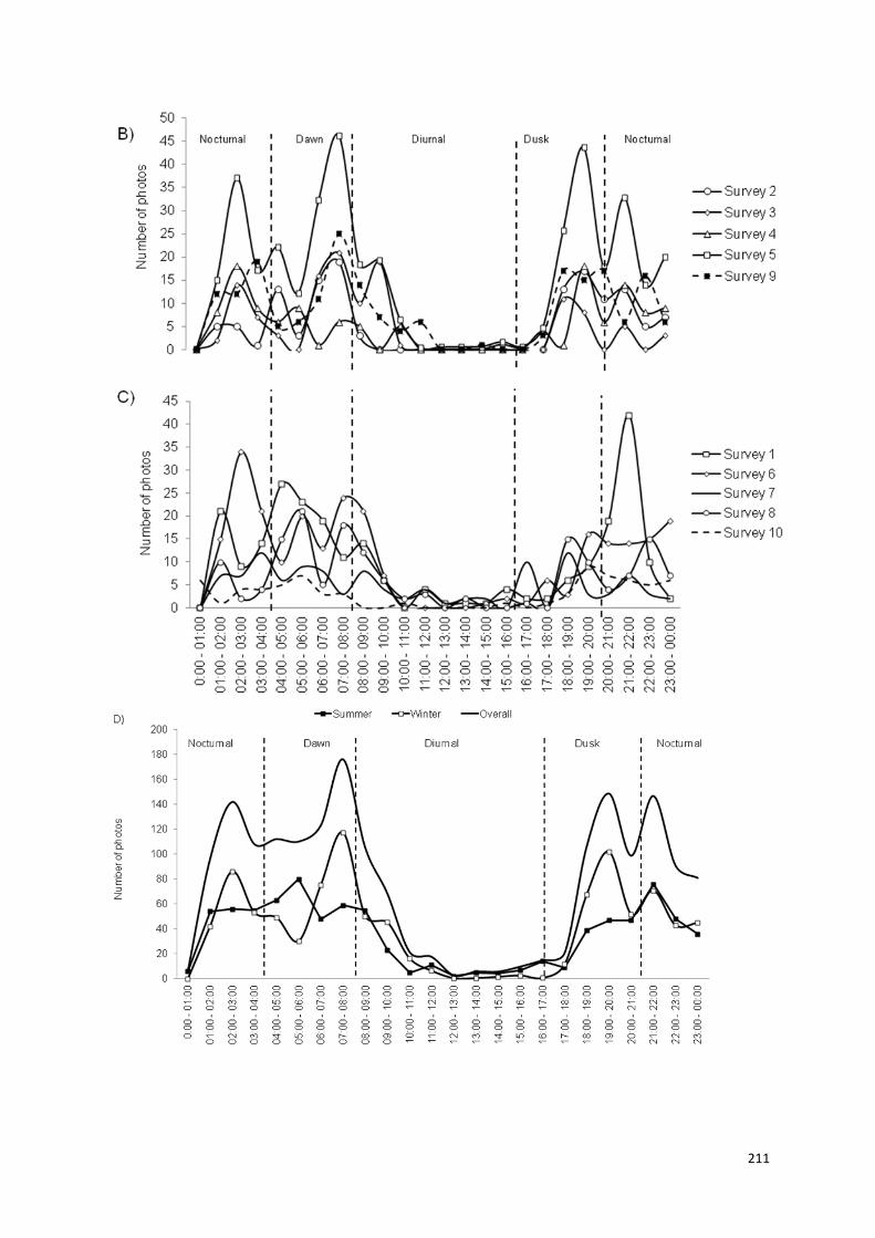
211
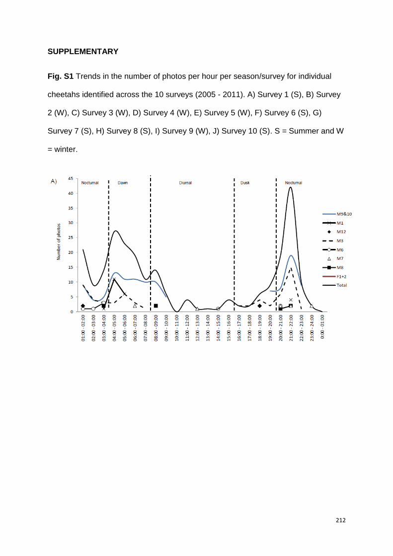
212
SUPPLEMENTARY
Fig. S1 Trends in the number of photos per hour per season/survey for individual
cheetahs identified across the 10 surveys (2005 - 2011). A) Survey 1 (S), B) Survey
2 (W), C) Survey 3 (W), D) Survey 4 (W), E) Survey 5 (W), F) Survey 6 (S), G)
Survey 7 (S), H) Survey 8 (S), I) Survey 9 (W), J) Survey 10 (S). S = Summer and W
= winter.
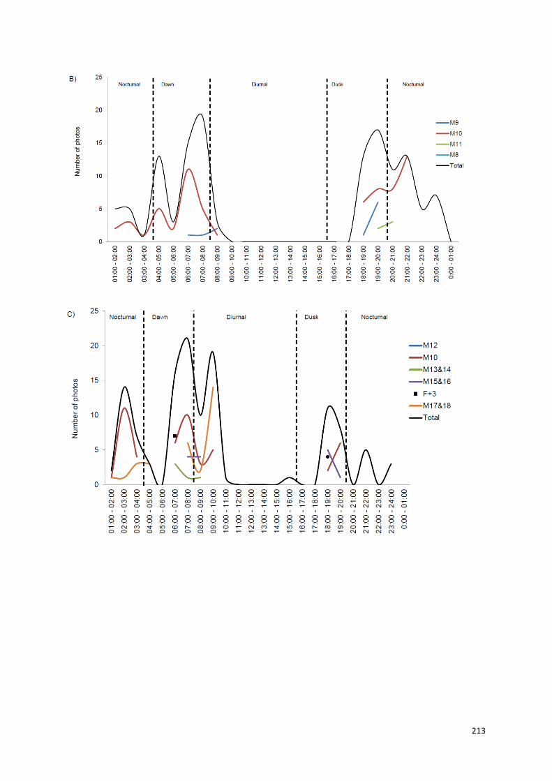
213
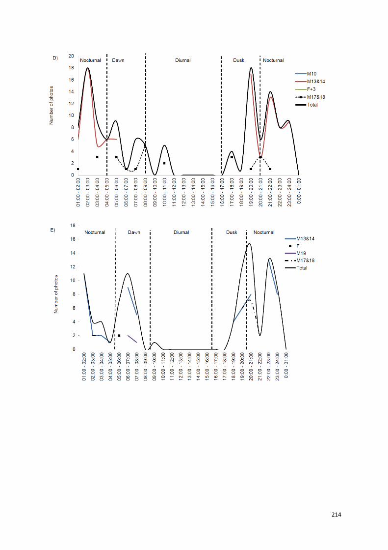
214

215
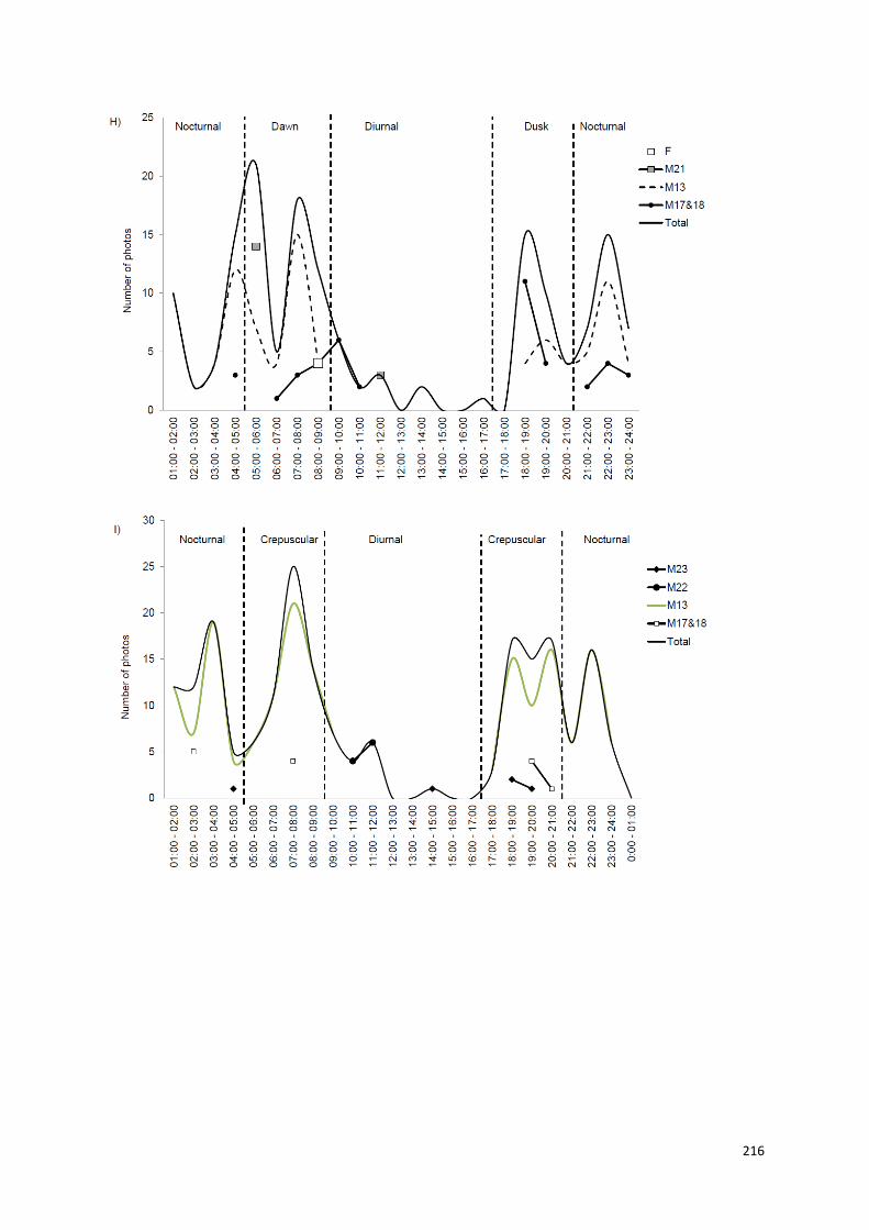
216
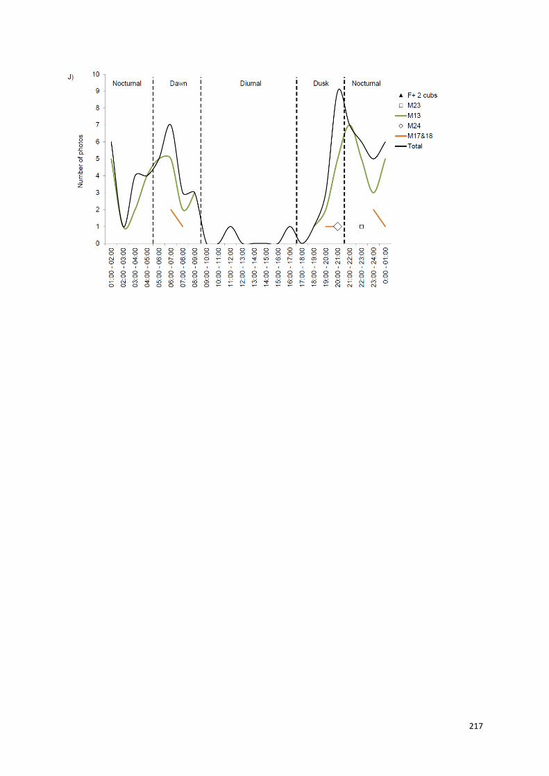
217
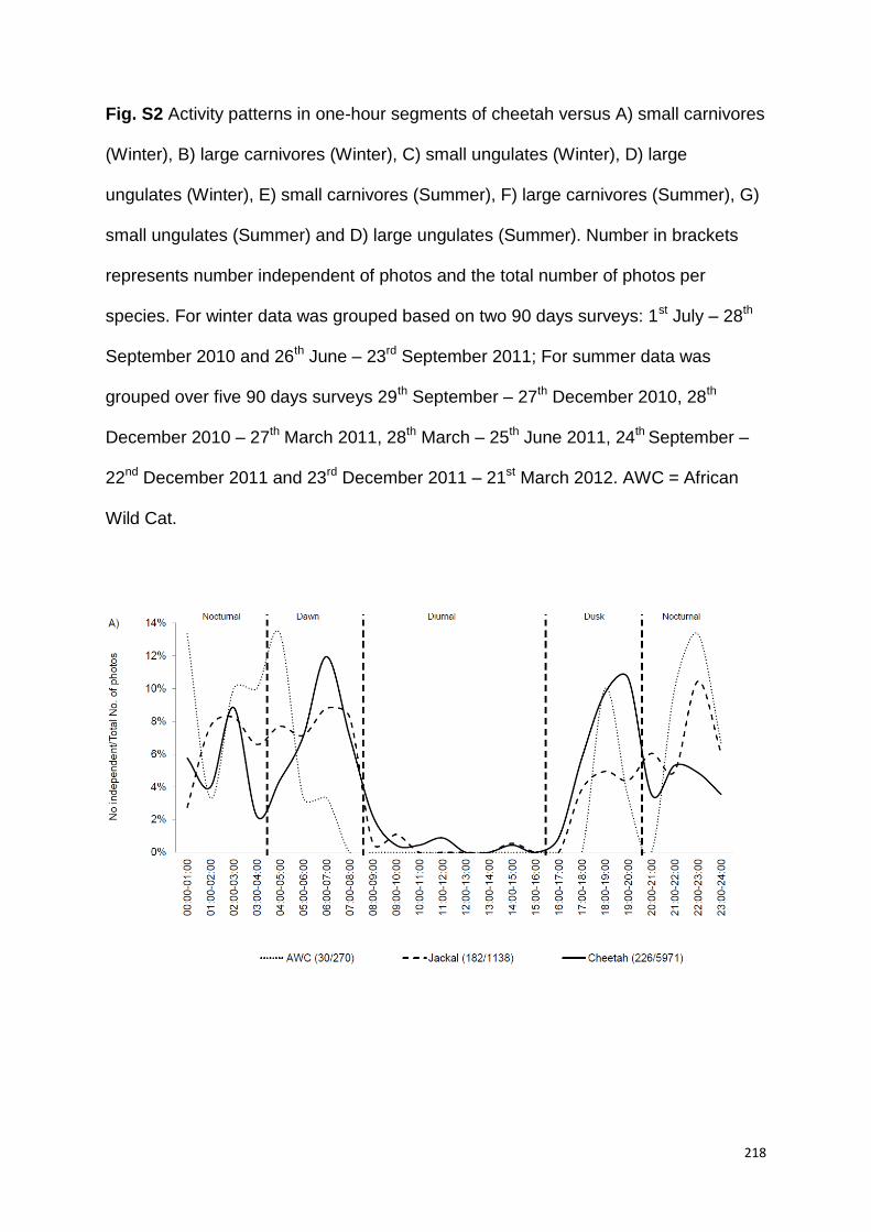
218
Fig. S2 Activity patterns in one-hour segments of cheetah versus A) small carnivores
(Winter), B) large carnivores (Winter), C) small ungulates (Winter), D) large
ungulates (Winter), E) small carnivores (Summer), F) large carnivores (Summer), G)
small ungulates (Summer) and D) large ungulates (Summer). Number in brackets
represents number independent of photos and the total number of photos per
species. For winter data was grouped based on two 90 days surveys: 1st July – 28th
September 2010 and 26th June – 23rd September 2011; For summer data was
grouped over five 90 days surveys 29th September – 27th December 2010, 28th
December 2010 – 27th March 2011, 28th March – 25th June 2011, 24th September –
22nd December 2011 and 23rd December 2011 – 21st March 2012. AWC = African
Wild Cat.
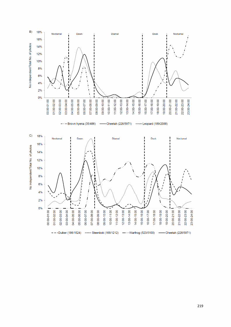
219
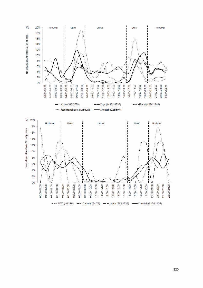
220
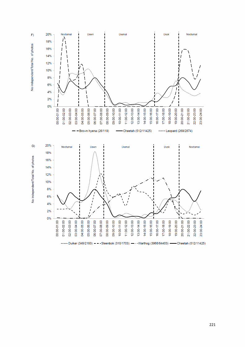
221
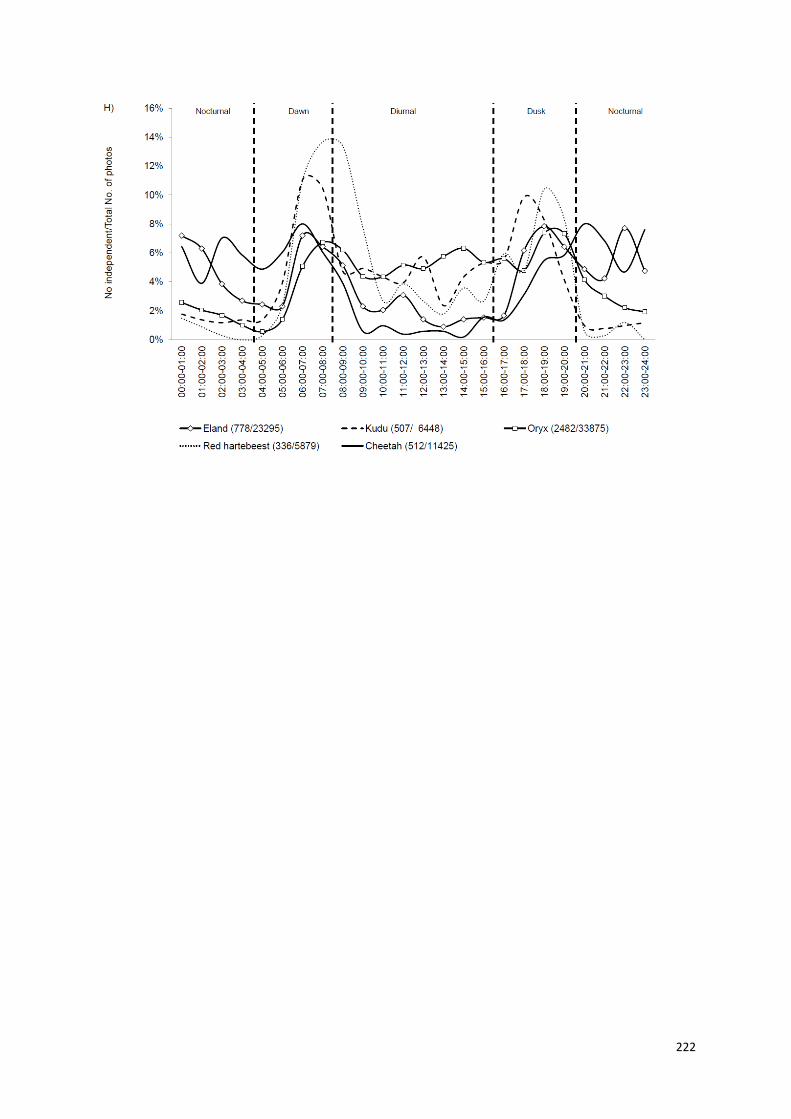
222
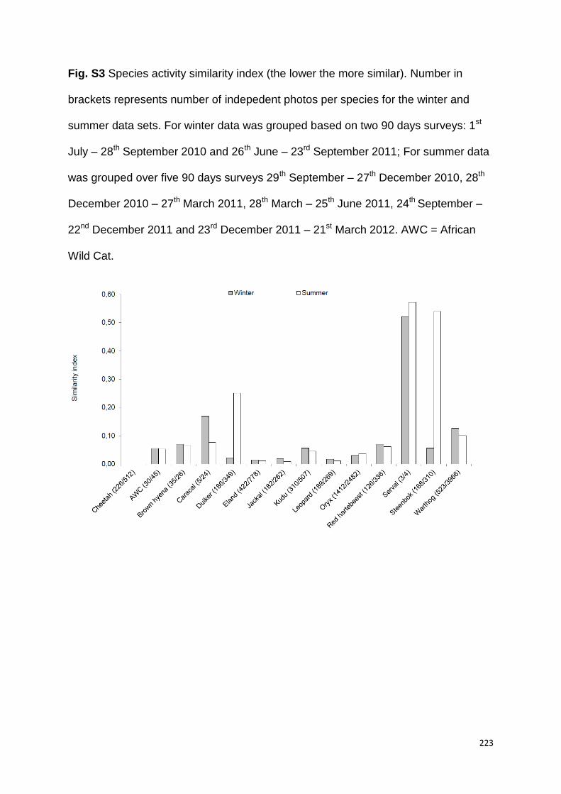
223
Fig. S3 Species activity similarity index (the lower the more similar). Number in
brackets represents number of indepedent photos per species for the winter and
summer data sets. For winter data was grouped based on two 90 days surveys: 1st
July – 28th September 2010 and 26th June – 23rd September 2011; For summer data
was grouped over five 90 days surveys 29th September – 27th December 2010, 28th
December 2010 – 27th March 2011, 28th March – 25th June 2011, 24th September –
22nd December 2011 and 23rd December 2011 – 21st March 2012. AWC = African
Wild Cat.

224
Capítulo VI
225
5.1 Discussão geral
O estudo concentrou-se na população de guepardos da Namibia, tendo como
objetivo geral a compreensão da demografia histórica e contemporânea desta
população e da espécie em geral, visando ao desenvolvimento de ações eficazes
para sua conservação e manejo, tendo em vista a existência de diversas ameaças à
sua sobrevivência, incluindo efeitos de mudancas climáticas globais. Para isto,
foram identificados três objetivos específicos, sendo eles: (1) uma avaliação
estatística da história demográfica desta população, em relação à variabilidade
climática do Quartenário e fatores antropogênicos; (2) uma estimativa e investigação
da interação entre o seu tamanho efetivo contemporâneo (Ne), taxas vitais e
viabilidade populacional de longo prazo; e (3) uma avaliação de tendências em
abundância e densidade.
Inicialmente, o estudo mostrou que a população tem uma história demográfica
complexa, com pelo menos três eventos de redução nos últimos 240 mil anos (kya),
corroborando sugestões anteriores de declínio no passado (O’Brien et al. 1985,
1987; Pimm et al. 1989; Menotti-Raymond e O'Brien 1994; Hedrick 1996; Driscoll et
al. 2002). Entretanto, cenários assumindo declínios e expansões severos não
tiveram probabilidades posteriores mais elevadas em relação aos cenários
postulando declínios graduais ou estabilidade em longo prazo. Os períodos de
modificação coincidem com os principais eventos climáticos ao longo do tempo
investigado, como os episódios periódicos de aridez, que ocorreram entre 135 kya -
90 kya (Cohen et al. 2007) condições de aridez pós LGM (26.5 a 19 kya) (Clark et
al. 2009) e aumento de aridez particularmente na Namíbia durante o período de
3500 a 300 anos atrás (Chase et al. 2010) . Tais eventos resultaram em alternância
das formas vegetacionais, conversão de florestas em pastagens e vice-versa (Gil-
226
Romera et al. 2007; Chase et al. 2009; Turpie et al. 2010) e redução ou extinção de
espécies de presas no sudoeste da África (Faith 2012; Osmers et al. 2012) e no
continente africano como um todo (Reed 1997; deMenocal 2004). A partir disso,
postulamos como causas prováveis de declínio, no caso das mudanças
demográficas ancestrais (i.e. no final da LGM e Holoceno inicial), a redução de
habitats adequados (i.e. disponibilidade de presas e estrutura da vegetação),
intensificação da competição interespecífica , periodicidade de mudanças na
vegetação e clima, ou uma combinação destes fatores. Situação semelhante parece
ter acontecido com a zebra-da-montanha do Cabo, na África do Sul (Equus zebra
zebra) (Faith 2012), cuja população pode não ter recuperado os níveis demográficos
anteriores a ~ 3600 anos atrás.
O efeito de fatores antropogênicos foi considerado mínimo até recentemente
(~ 1000-300 anos) devido à baixa população humana na Namibia (i.e. < 500.000 em
1950) (Wikipedia 2013). O setor agrícola na região só se intensificou durante os
últimos 1000 anos (Araki 2005), quando a paisagem se degradou (Mendelsohn
2006), as terras de cultivo tornaram-se mais áridas (Araki 2005) e alguns carnívoros
(i.e. leões Panthera leo e hienas Crocuta crocuta) foram reduzidos severamente ou
eliminados (Marker Kraus et al. 1996; Nowell 1996; Werner 1993),sugerindo a
influência dos fatores antropogênicos. Uma conclusão semelhante foi obtida para os
tigres na Índia (~ 600 anos) (Mondol et al. 2009). Adicionalmente, a falta de sinais
de declínio nos últimos 300 anos não descarta os impactos genéticos devido a
causas antropogênicas. De fato, durante o século passado, a caça furtiva provocou
períodos de acentuada deriva genética em elefantes (Okello et al. 2008) e a caça
descontrolada reduziuem em cinco vezes o tamanho efetivo (Ne) da população de
crocodilos (Crocodylus niloticus) (Bishop et al. 2009). Este é provavelmente o caso
227
da população de estudo, a qual diminuiu (população de censo Nc) durante o século
passado devido a fatores diversos (e.g. secas, reduções de presas devido a
epidemias de raiva e conflitos com os humanos) (Marker-Kraus et al. 1996; Marker
et al. 2010).
Posteriormente, o estudo demonstrou que a população parece ser viável em
longo prazo (Ne de 450 - 2500), com base em simulações que integram traços da
história de vida. Estimativas baseadas em estimadores genéticos (LDNe,
ONeSAMP, DIYABC, e MSVAR1.3) foram menores. Para approximar Ne a o
tamanho geracional, a estimativa combinada de LDNe e de ONeSAMP foi
multiplicada por tempos de geração (G) (como em Hare et al. 2010). Utilizando a
proporção observada mínima de 0.21 (Ne/Nc) isso seria equivalente a um Nc de
2143 - 11905 indivíduos (ou 2686 - 6314 95% CI baseado na estimativa combinada
de LDNe e ONeSAMP). Valores maiores podem ser esperados se Ne/Nadultos mínima
de 0,40 for considerada. Portanto, em seu tamanho atual a população não está em
risco severo de extinção devido a um baixo potencial evolutivo, visto que Ne é maior
que o valor teórico de 500 frequentemente considerado na literatura (Allendorf e
Luikart 2007). No entanto, essa viabilidade é suscetível a diferentes fatores.
Observamos que Ne foi influenciada positivamente por uma série de fatores,
incluindo o G utilizado e conseqüentemente fatores que influenciam a sua média
(por exemplo, diminuição de mortalidade de machos adultos). Os fatores incluem
diminuições baixas (~ 10%) na proporção de fêmeas reprodutoras e decréscimos
moderados (~20%) na taxa de mortalidade de fêmeas adultas acompanhadas ou
não de filhotes e/ou juvenis. Reduções no tamanho inicial da população (Ninit)
também influenciaram positivamente o Ne. Estes fatores também influenciaram
positivamente Nc ou Nadultos e o tempo médio de G, mas se diferenciaram em ordem
228
de impacto e magnitude. Por exemplo, declínios de 10% na proporção de fêmeas
reprodutoras e 20% em Ninit afetaram Ne e Nc positivamente, mas o impacto do
primeiro foi maior em Ne do que em Nc, e vice-versa para Ninit. Em geral, alguns
destes resultados são suportados pela literatura.
Primeiramente, embora os Nc inferidos não devam ser tomados pelo valor
nominal, as estimativas estão de acordo com a literatura (Hanssen & Stander 2004;
Marker et al. 2007; Purchase et al. 2007; o que é sugestivo de uma estimativa
consistente deste parâmetro. Segundo, assim como Palstra and Palstra (2010) e
Andrello et al. (2012), ações de conservação influenciam positivamente e por vezes
concomitantemente, a diversidade genética da população (heterozigosidade), Nc,
taxa de crescimento e G. Terceiro, observou-se um aumento no Ne devido a uma
redução na mortalidade de filhotes e juvenis (i.e. maior sucesso reprodutivo)
combinada a um aumento em G (devido aos aumentos moderados na sobrevivência
de adultos) da mesma forma que o observado em bisões (Bison bison) (Pérez-
Figueroa et al. 2012). Nossos resultados, como os de Peréz-Figueroa et al. ( 2012),
diferenciam-se dos de Saether et al. (2009), que observaram um aumento na deriva
genética anual de alces americanos (Alces alces) com aumentos na sobrevivência
de filhotes (Ne diminui). Quarto, Ne/Nc (0,21) ou Nadulto (0,40) estão dentro do âmbito
empírico de valores medianos de 0.231 e 0,225 (Palstra e Fraser 2012) e
estimativas teóricas de 0.5 ou 0.25 e 0.75 (Nunney 1991; Nunney 1993; Nunney e
Elam 1994). Esta proporção tambem foi influenciada pelo tipo de N utilizado e G
(Waite e Parker 1996; Lee et al. 2011; Palstra e Fraser 2012). Quinto, os padrões
observados nas taxas de sobrevivência de machos parecem resultar em um número
maior gamético, cuja influência final no Ne é condicionada à distribuição de
remoções em relação ao status de reprodução ou classe de idade (Storz et al.
229
2001). Por fim, reduções moderadas (~20%) na proporção de fêmeas reproduzindo
podem também reduzir Ne (Saether et al. 2009). Enfim, as diferenças observadas
em Ne devido a níveis de perturbações diferentes em taxas vitais indicam que os
impactos não são lineares (Stott et al. 2012), mas que ações de conservação
orientadas para Nc também podem influenciar Ne positivamente.
O estudo mostrou que as estimativas de densidade de adultos no centro-
norte da Namíbia variaram entre 5 - 20 km-2 e foram significativamente semelhantes
entre diferentes estações. Esta semelhança parece ser resultado da dinâmica das
áreas de vida (devido à estabilidade social) associada à capacidade-suporte na
escala amostrada. A abundância variou em uma média de 9 ± 7 indivíduos adultos
por amostragem, com flutuações guiadas por indivíduos não residentes (30 de um
total de 39 indivíduos adultos). Animais residentes (n = 9) tiveram a posse das áreas
de vida dos três aos seis ou mais anos (i.e. idade adulta), com base em sua
utilização das estações de marcação olfativa de 6 a 48 meses (31 ± 17), com uma
visita de guepardo por estação a cada 5 ± 8 dias em média. Os padrões de
atividade mostraram um comportamento noturno que coincide com o padrão
observado em espécies de ungulados e carnívoros simpátricos, mas com menos
capturas durante o inverno.
Indivíduos residentes foram capturados mais frequentemente em estações
localizadas no centro de suas áreas de vida, visitando outras áreas com menor
freqüência. Novos recrutas mostraram padrões similares de utilização do espaço em
relação a seus antecessores (e.g. um único macho com uma coalizão de dois
machos durante dois anos). Os padrões observados foram semelhantes entre
indivíduos monitorados por radiotelemetria e entre indivíduos monitorados por
armadilhas fotográficas. Novos recrutamentos ocorrerm em duas oportunidades:
230
uma devido a um território vago pela morte de uma coalizão no ano anterior, e a
outra devido ao possível deslocamento de um macho solitário por uma coalizão de
dois indivíduos após dois anos de sobreposição espacial. Observou-se uma razão
sexual desigual de 4:1 em favor dos machos. Fêmeas acompanhadas de filhotes
(2.5 ± 0.57, n = 15) foram mais frequentemente capturadas do que fêmeas solitárias
(n = 1), sendo as capturas mais frequentes durante o verão. Alguns dos resultados
ecológicos e comportamentais para essa população estão sendo reportados pela
primeira vez, mas são condizentes com as informações encontradas na literatura
para a espécie.
As estimativas de densidade deste estudo foram semelhantes às de estudos
que utilizaram questionários ( Hanssen e Stander 2004). A estrutura demográfica
limitada na escala amostrada não é exclusiva deste estudo (O'Connell et al. 2011),
embora o nosso período de amostragem seja superior ao de outros trabalhos
utilizando armadilhas fotográficas (e.g. Maffei 2011). O período de posse de uma
área própria é semelhante à relatada em guepardos no Serengeti, baseado em
estudos comportamentais de longo prazo, de 4 a 36 meses (Caro e Collins 1987;
Caro e Kelly 2001). Esta fidelidade ao longo das estações é apoiada pela falta de
efeito sazonal sobre o tamanho das áreas de vida de guepardos na área de estudo
(Marker et al. 2008). Embora esteja baseado em uma amostra pequena, os efeitos
da estrutura social de grupo e da saúde dos animais como mecanismos de retenção
de áreas próprias de vida estão relacionados, através do possível deslocamento de
um macho solitário por uma coalizão e do afastamento dos não-residentes por
machos solitários (> 3 anos). Finalmente, houve semelhanças nos padrões de uso
espacial por novos recrutas e antecessores (em tempos sem sobreposição) e
frequências maiores de visitação em estações localizadas ao centro de areas de
231
vida por indivíduos monitorados por radiotelemetria, assim como em hienas no
Kalahari (Mills et al. 1980). Isto sugere o papel de pistas olfativas na demarcação,
forrageamento ou orientação de indivíduos aos locais de marcação, bem como de
familiarização de habitat (Eisenberg & Kleiman, 1972; Gorman e Trowbridge 1989;
Potts et al. 2012). Estes aspectos são englobados pela teoria de utilização dos
recursos (Gittleman 1989). Eaton (1970) indica que o sistema de marcação de
guepardos é primariamente um mecanismo que permite a coexistência de vários
indivíduos dentro da mesma área ("time-plan").
O padrão temporal noturno e crepescular está de acordo com estudos
prévios (Marker, Fabiano e Nghikembua 2008; Cozzi et al. 2012) mas diferencia-se
do geralmente considerado para a espécie, diurno (Durant 2000; Hayward and
Slotow 2009). Cozzi et al. (2012) indica que este movementos de guepardos é
influenciado por ciclos lunares. Fundamentalmente, estes dados suportam que esta
característica é filogenetica (Holt 2009) visto que outros grande carnívores como o
leão, leopardo, hienas e wild dog tambem apresentão um padrão semelhante
(Hayward & Slotow 2009; Cozzi et al. 2012).
5.2 Implicações para conservação e manejo
Os resultados do estudo têm diversas implicações para a conservação. Primeiro: os
efeitos ilustrados da variabilidade climática e instabilidade ambiental (e.g.
aridificação) sobre a demografia desta população e possivelmente de outras
populações do sul da África durante o Pleistoceno e Holoceno sugerem que a
viabilidade e persistência desta população está condicionada às potenciais ameaças
impostas por alterações climáticas futuras e as suas interações com as práticas de
232
uso da terra (Turpie et al. 2010). Portanto, existe uma necessidade de compreensão
mais profunda do impacto das alterações climáticas essencialmente em relação à
segurança alimentar, visto que estudos sugerem uma perda potencial de
produtividade, podendo fomentar uma reversão para níveis menores de tolerância
aos carnívoros (Marker et al. 2010; Turpie et al. 2010). Tal situação é de grande
importância dado que não detectamos nenhum sinal de expansão dentro do período
avaliado.
Segundo: as ações de conservação deveriam concentrar-se particularmente
em aspectos relacionados a fêmeas, especialmente aquelas em idade reprodutiva,
para maximizar o potencial evolutivo populacional. Além disso, como Ne foi sensível
a reduções na proporção de fêmeas reprodutoras e na capacidade suporte,
respectivamente, esforços devem ser orientados para monitorar tendências destas
variáveis.
Finalmente: os nossos resultados reforçam as ações de conservação atuais
de soltura de indivíduos nos locais de captura (Marker et al. 2003; Marker et al.
2008) sempre que possível, e logo após a remoção. Isto se deve à alta fidelidade
territorial, ao fluxo de indivíduos não residentes e possívies reduções na variância
reprodutiva masculina que podem afetar Ne e, portanto, a viabilidade genética da
população.
5.3 Concluções e recomendações
Em resumo, o estudo constatou que a população de guepardos da Namíbia é
provavelmente viável em longo prazo, e as análises de sensibilidade sugerem que
233
os esforços de conservação devem continuar a se concentrar principalmente em
aspectos relacionados à sobrevivência das fêmeas, seguidos pela dos machose
pelos juvenis/não-reprodutivos. Um efeito colateral destas medidas é a estabilidade
social e conseqüentemente, a dinâmica das áreas de vida que parece regular a
densidade, pelo menos dos machos. Isto é importante à medida que a instabilidade
social pode modificar os padrões de acasalamento, afetando o tamanho efetivo
populacional ou sua razão com o tamanho total do censo. A diversidade genética da
população estudada, e possivelmente a da África austral como um todo,resultam de
uma complexa história caracterizada por fases de estabilidade intercaladas por
períodos de declínio, com a contribuição de variações climáticas e instabilidade
ambiental, juntamente com a competição interespecífica. Quanto ao papel dos
fatores antropogênicos, especialmente durante o período estável (300 aa até o
presente), são necessárias avaliações adicionais, como a detecção de possíveis
sinais transitórios ao nível de coorte. De um modo geral, a persistência e viabilidade
da população parece estar relacionada predominantemente a efeitos diretos e
indiretos das mudanças climáticas.
Estudos futuros devem explorar a conexão entre a ocupação e distribuição da
população e como elas serão provavelmente afetadas pelas tendências projetadas
de mudanças climáticas. Isto não deve restringir-se a uma espécie única, mas deve
incorporar múltiplas espécies de carnívoros e a sua base de presas. Há também a
necessidade urgente de estudos para elucidar o sistema de acasalamento desta
população (e.g. Gotelli et al. 2007) bem como estudos comportamentais das
fêmeas, os quais.forneceriam uma nova compreensão dos processos que afetam
Ne e Nc (dinâmica populacional). Por fim, há necessidade de estudos de longo
prazo abrangendo áreas maiores, utilizando métodos sistemáticos de levantamento,
234
e de uma continuada integração deste tipo de informação com aquelas geradas por
análises genéticas detalhadas e simulações computacionais de cenários cada vez
mais realistas envolvendo esta e outras populações da espécie.
Referências
Allendorf FW, Luikart G (2007) Conservation and the Genetics of Populations.
Blackwell, USA
Andrello M, Nicolè F, Till-Bottraud I, Gaggiotti OE (2012) Effect of Stage-Specific
Vital Rates on Population Growth Rates and Effective Population Sizes in an
Endangered Iteroparous Plant. Conserv Biol 26:208–217
Araki S (2005) Change in population and land-use intensities in several villages of
the four northern regions of Namibia. ASM 30:77–88
Bishop, J M., Leslie, A.J., Bourquin, S.L., & O’Ryan, C. (2009). Reduced effective
population size in an overexploited population of the Nile crocodile (Crocodylus
niloticus). Biol Conserv 142: 2335–2341
Caro TM, Kelly M (2001) Cheetahs and their mating system. In L. Dugatkin, ed.
Model Systems in Behavioral Ecology. Princeton University Press, pp 512 – 532
Caro TM, Collins DA (1987) Male Cheetah Social Organization and Territoriality.
Ethology 74:52–64
Chase BM, Meadows ME, Scott L, Thomas DSG, Marais E, Sealy J, Reimer PJ
(2009) A record of rapid Holocene climate change preserved in hyrax middens
from southwestern Africa. Geology 37:703–706
235
Chase BM, Meadows ME, Carr AS, Reimer PJ (2010) Evidence for progressive
Holocene aridification in southern Africa recorded in Namibian hyrax middens:
Implications for African Monsoon dynamics and the “‘African Humid Period’”.
Quatern Res 74:36–45
Clark PU, Dyke AS, Shakun JD, Carlson AE, Clark J, Wohlfarth B, Mitrovica JX
(2009) The Last Glacial Maximum. Science 325:710–4
Cohen AS, Stone JR, Beuning KRM, Park LE, Reinthal PN, Dettman D, Scholz CA
(2007) Ecological consequences of early Late Pleistocene megadroughts in
tropical Africa. PNAS pp. 6–11 doi/10.1073/pnas.0703873104
Cozzi G, Broekhuis F, McNutt JW, Turnbull L, Macdonald D, Schimid B (2012) Fear
of the dark or dinner by moonlight ? Reduced temporal partitioning among
Africa’s large carnivores. Ecology 93: 2590–2599
deMenocal PB (2004) African climate change and faunal evolution during the
Pliocene–Pleistocene. Sci Lett 220:3–24
Driscoll CA, Menotti-Raymond M, Nelson G, Goldstein D, O’Brien SJ (2002)
Genomic microsatellites as evolutionary chronometers: a test in wild cats.
Genome Res 12:414–23
Eaton RL (1970) Group interactions, spacing and territoriality in cheetahs.
Zeitschrift für Tierpsychologie 27:481-91
Eisenberg JF, Kleiman DG (1972) Olfactory communication in mammals. Annu Rev
Ecol Syst 3:1–32
236
Eitel B, Eberle J, Kuhn R (2002) Holocene environmental change in the Otjiwarongo
thornbush savanna (Northern Namibia): evidence from soils and sediments.
Catena 47: 43–62
Faith JT (2012) Palaeozoological insights into management options for a threatened
mammal: southern Africa’s Cape mountain zebra (Equus zebra zebra). Divers
Distrib 18 438–447.
Gil-Romera G, Scott L, Marais E, Brook GA ( 2007) Late Holocene environmental
change in the northwestern Namib Desert margin: New fossil pollen evidence
from hyrax middens. Palaeogeogr Palaeoclimatol Palaeoecol 249:1–17
Gittleman LL (1989) (ed) Canrivore Behaviour Ecology and Evolution, Cornell
University
Gorman ML, Trowbridge BJ (1989) The role of Odor in the Social Lives of
Carnivores. In LL Gittleman (ed) Canrivore Behaviour Ecology and Evolution,
Cornell University, pp 57-88
Gottelli D, Wang J, Bashir S, Durant SM (2007) Genetic analysis reveals promiscuity
among female cheetahs. Proc R Soc B 274:1993–2001
Hanssen L, Stander P (2004) Namibia large carnivore atlas, Windhoek, Namibia
Hare MP, Nunney L, Schwartz MK, Ruzzante DE, Burford M, Waples RS, Ruegg K
(2010) Understanding and Estimating Effective Population Size for Practical
Application in Marine Species Management. Conserv Biol doi 10.1111/j.1523-
1739.2010.01637.x
237
Hayward MW, Slotow R (2009) Temporal partitioning of activity in large African
carnivores : tests of multiple hypotheses. S Afr J Wildl Res 39:109–125
Hedrick PW (1996) Bottleneck (s) in Cheetahs or Metapopulation. Conserv Biol
10:897–899
Holt RD (2009) Bringing the Hutchinsonian niche into the 21st century: ecological
and evolutionary perspectives. PNAS 106 Suppl 19659–65.
doi:10.1073/pnas.0905137106
Lee AM, Engen, Sæther B-E, Engen B (2011) The influence of persistent individual
differences and age at maturity on effective population size Subject collections
The influence of persistent individual differences and age at maturity on effective
population size. Proc R Soc B doi:10.1098/rspb.2011.0283
Maffei L, Polisar J, Garcia R, Jose M, Noss AJ (2011) Perspectives from ten years of
jaguar (Panthera onca) camera trapping in mesoamerica. Mesoamericana
15:49–59
Marker LL, Dickman AJ, Mills MGL, Macdonald DW (2010) Cheetahs and ranchers
in Namibia : a case study. In D. MacDonald & A. Loveridge (eds) Biology and
Conservation of Wild Felids. Oxford University Press, UK, pp 353 – 372
Marker LL, Dickman AJ, Mills MGL, Jeo RM, Macdonald DW (2008) Spatial ecology
of cheetahs on north-central Namibian farmlands. J Zool 274: 226–238
Marker L, Dickman AJ, Wilkinson C, Schumann B, Fabiano E (2007) The Namibian
Cheetah : Status Report. Cat News, Special Issue 3:4–13
238
Marker LL, Dickman AJ, Jeo RM, Mills MGL, Macdonald DW (2003) Demography of
the Namibian cheetah , Acinonyx jubatus jubatus. Biol Conserv 114:413–425
Marker-Kraus L, Kraus D, Barnett D, Hurlbut S (1996) Cheetah survival on
Namibian farmlands. Cheetah Conservation Fund, Windhoek
Mendelsohn J (2006) Farming Systems in Namibia. ABC Press, South Africa
Menotti-Raymond MA, O’Brien SJ (1994) Evolutionary conservation of ten
microsatellite loci in four species of Felidae. J Hered 86:319–22
Mills MGL, Gorman ML, Mills MEJ (1980) The scent marking behaviour of the brown
hyena, Hyena brunnea, in the Southern Kalahari. South African J Zool 15:240-
248
Mondol S, Karanth KU, Ramakrishnan U (2009) Why the Indian subcontinent holds
the key to global tiger recovery. PLoS genetics 5: p.e1000585
Nowell K (1996) Namibian Cheetah Conservation Strategy. Windhoek, Namibia
Nunney L (1991) The influence of age structure and fecundity on effective population
size. Proc R Soc B 246:71–6
Nunney L (1993) The Influence of Mating System and Overlapping Generations on
Effective Population Size. Evolution 47:1329–1341
Nunney L, Elam DR (1994) Estimating the effective population ise of conserved
populations. Conserv Biol 8:175–184
239
O’Brien SJ, Wildt DE, Bush M, Caro TM, FitzGibbon C, Aggundey I, Leakey RE
(1987) East African cheetahs: evidence for two population bottlenecks? PNAS
84:508–11
O’Brien SJ, Roelke ME, Marker LL, Newman A, Winkler CA, Meltzer D, Colly L
(1985) Genetic basis for species vulnerability in the cheetah. Science 227:1428–
1434
O'Connell AF, Nichols JD, Karanth UK (2011) Camera traps in Animal Ecology
Methods and Analyses. A. F. O’Connell, J. D. Nichols, & K. U. Karanth, eds.,
Springer US
Okello JBA, Wittemyer G, Rasmussen HB, Arctander P, Nyakaana S, Douglas-
Hamilton I, Siegismund HR (2008) Effective population size dynamics reveal
impacts of historic climatic events and recent anthropogenic pressure in African
elephants. Mol Ecol 17:3788–99
Osmers B, Petersen B, Hartl GB, Grobler JP, Kotze A, Aswegen E Van, Zachos FE
(2012) Genetic analysis of southern African gemsbok (Oryx gazella) reveals
high variability , distinct lineages and strong divergence from the East African
Oryx beisa. Mamm Biol 77: 60–66
Palstra FP, Ruzzante DE (2010) A temporal perspective on population structure and
gene flow in Atlantic salmon (Salmo salar) in Newfoundland, Canda. Can J Fish
Aquat Sci 67:225-242
Palstra FP, Fraser DJ (2012) Effective / census population size ratio estimation : a
compendium and appraisal. Ecology and Evolution 2:2357–2365
240
Pérez-Figueroa A, Wallen RL, Antao T, Coombs JA, Schwartz MK, White PJ, Luikart
G (2012) Conserving genomic variability in large mammals: Effect of population
fluctuations and variance in male reproductive success on variability in
Yellowstone bison. Biol Conserv 150:159–166
Pimm SL, Gittleman JL, McCracken GF, Gilpin M (1989) Plausible alternatives to
bottlenecks to explain reduced genetic diversity. TREE 4:176–178
Potts JR, Harris S, Giuggioli L (2012) Territorial dynamics and stable home range
formation for central place foragers. PloS one 7: p.e34033
Purchase G, Marker LL, Marnewick K, Klein R, Williams S (2007) Regional
Assessment of the Status , Distribution and Conservation Needs of Cheetahs in
Southern Africa. Cat News Special Issue 3: 44–46
Reed KE (1997) Early hominid evolution and ecological. Journal of Human Evolution
32:289–322
Saether B-E, Engen S, Solberg EJ (2009) Effective size of harvested ungulate
populations. Anim Conserv 12:488–495
Smith JLD, Mcdougal C, Miquellet D (1989) Scent marking in free-ranging tigers,
Panthera tigris. Anim Behav 37:1–10
Storz JF, Bhat HR, Kunz TH (2001) Genetic Consequences of Polygyny and Social
Structure in an Indian Fruit Bat , Cynopterus sphinx . II . Variance in Male
Mating Success and Effective Population Size. Evolution 55:1224–1232
241
Stott I, Hodgson DJ, Townley S (2012) Beyond sensitivity: nonlinear perturbation
analysis of transient dynamics. Methods in Ecology and Evolution 3:673–684
Turpie AJ, Midgley G, Brown C, Barnes J, Pallett J, Desmet P, Tarr J, Tarr P (2010)
Climate Change Vulnerability and Adaptation Assessment for Namibia’s
Biodiversity and Protected, Windhoek
Waite TA, Parker PG (1996) Dimensionless Life Histories and Efective Size
Population. Conserv Biol 10: 1456–1462
Werner W (1993) A Brief History of Land Disposession in Namibia. JSAS 19: 1–12
Wikipedia (2013) Demographics of Namibia. Wikipedia, The Free Encyclopedia.
Available at:
http://en.wikipedia.org/w/index.php?title=Demographics_of_Namibia&oldid=532
446073 [Accessed February 25, 2013]