UNIVERSITY OF SÃO PAULO

Institute of Astronomy, Geophysics, and Atmospheric Sciences

Department of Atmospheric Sciences

MARCO AURÉLIO ALVARENGA ALVES

Investigation of the energy balance and momentum flux in the

atmospheric surface layer of a non-glaciated coastal area at

Ferraz Station, Antarctic region

Investigação do balanço de energia e do fluxo de momento na camada

limite atmosférica em uma região costeira não glaciada na Estação

Ferraz, região Antártica

São Paulo

2016

MARCO AURÉLIO ALVARENGA ALVES

Investigation of the energy balance and momentum flux in the atmospheric surface

layer of a non-glaciated coastal area at Ferraz Station, Antarctic region

Investigação do balanço de energia e do fluxo de momento na camada limite

atmosférica em uma região costeira não glaciada na Estação Ferraz, região

Antártica

(VERSÃO CORRIGIDA)

A dissertation submitted in partial fulfilment of

the requirements for the degree of Master of

Science in Meteorology.

Advisor: Univ.-Prof. Dr. Jacyra Soares

São Paulo

2016

iv

v

Acknowledgements

I would like to acknowledge with sincere thanks many people who have

supported and assisted this research: my advisor Dr. Jacyra Soares for her time, patience,

motivation, and friendship during these two years working together. My thesis would not

have been possible without her; the professional team of LI-COR (Lincoln, Nebraska -

USA), especially Dr. Jiahong Li, for his precious help with the high frequency system

measurements used in this study; Georgia Codato for her availability with the data I used

in this study. In addition to my thesis, I also express my gratitude to several friends and

colleagues at IAG, who provided me assistance in times of need and personal support:

Leonardo Domingues, Kátia Barros, Miriam Gigi, Thomas Martin, Jenniffer Guerra,

Odete Macie, Bionídio Banze, Cristina Arriaga, Eleazar Angulo, Luana Macedo, Dámian

Guevara, Hudson Lodi, and Caio Ruman. My family has been there for me throughout

my graduate career and I owe my overall success to their unconditional support.

I would like to thank CAPES for the scholarship. I acknowledge the financial

support offered by the INCT-APA and CNPq (Process 407137/2013-0 of the ETA

Project).

vi

vii

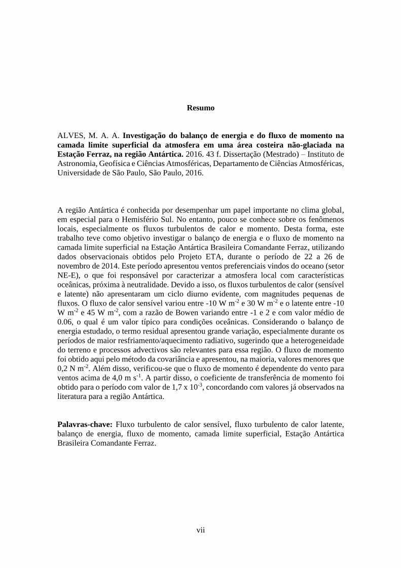
Resumo

ALVES, M. A. A. Investigação do balanço de energia e do fluxo de momento na

camada limite superficial da atmosfera em uma área costeira não-glaciada na

Estação Ferraz, na região Antártica. 2016. 43 f. Dissertação (Mestrado) – Instituto de

Astronomia, Geofísica e Ciências Atmosféricas, Departamento de Ciências Atmosféricas,

Universidade de São Paulo, São Paulo, 2016.

A região Antártica é conhecida por desempenhar um papel importante no clima global,

em especial para o Hemisfério Sul. No entanto, pouco se conhece sobre os fenômenos

locais, especialmente os fluxos turbulentos de calor e momento. Desta forma, este

trabalho teve como objetivo investigar o balanço de energia e o fluxo de momento na

camada limite superficial na Estação Antártica Brasileira Comandante Ferraz, utilizando

dados observacionais obtidos pelo Projeto ETA, durante o período de 22 a 26 de

novembro de 2014. Este período apresentou ventos preferenciais vindos do oceano (setor

NE-E), o que foi responsável por caracterizar a atmosfera local com características

oceânicas, próxima à neutralidade. Devido a isso, os fluxos turbulentos de calor (sensível

e latente) não apresentaram um ciclo diurno evidente, com magnitudes pequenas de

fluxos. O fluxo de calor sensível variou entre -10 W m-2 e 30 W m-2 e o latente entre -10

W m-2 e 45 W m-2, com a razão de Bowen variando entre -1 e 2 e com valor médio de

0.06, o qual é um valor típico para condições oceânicas. Considerando o balanço de

energia estudado, o termo residual apresentou grande variação, especialmente durante os

períodos de maior resfriamento/aquecimento radiativo, sugerindo que a heterogeneidade

do terreno e processos advectivos são relevantes para essa região. O fluxo de momento

foi obtido aqui pelo método da covariância e apresentou, na maioria, valores menores que

0,2 N m-2. Além disso, verificou-se que o fluxo de momento é dependente do vento para

ventos acima de 4,0 m s-1. A partir disso, o coeficiente de transferência de momento foi

obtido para o período com valor de 1,7 x 10-3, concordando com valores já observados na

literatura para a região Antártica.

Palavras-chave: Fluxo turbulento de calor sensível, fluxo turbulento de calor latente,

balanço de energia, fluxo de momento, camada limite superficial, Estação Antártica

Brasileira Comandante Ferraz.

viii

ix

Abstract

ALVES, M. A. A. Investigation of the energy balance and momentum flux in the

atmospheric surface layer of a non-glaciated coastal area at Ferraz Station, Antarctic

region. 2016. 43 p. Dissertation (Master degree) – Institute of Astronomy, Geophysics, and

Atmospheric Sciences, Department of Atmospheric Sciences, University of São Paulo, São

Paulo, 2016.

The Antarctic region is known for playing an important role in the global climate, especially to

the Southern Hemisphere. However, little is known about local atmosphere, especially the

turbulent fluxes of heat and momentum. Thus, this study aimed to investigate the energy

balance and the momentum flux in the atmospheric surface layer at the Brazilian Antarctic

Station “Comandante Ferraz”, using observational data obtained by ETA Project during the

period 22-26 November 2014. During this period, most of winds was from the ocean (NE-E

sector), characterizing the local atmosphere as oceanic and with stability near the neutrality.

Because of this, turbulent heat fluxes (sensible and latent) did not have a clear diurnal cycle,

with fluxes of small intensities. The sensible heat flux ranged from -10 W m-2 and 30 W m-2

and the latent -10 W m-2 and 45 W m-2, with the Bowen ratio ranging between -1 and 2 and

value average 0.06, which is a typical value for ocean conditions. Considering the studied

energy balance, the residual term showed large variations, especially during periods with large

radiative cooling/heating, suggesting that the heterogeneity of the surface and advective

processes are relevant to this region. The momentum flux was obtained here by the covariance

method and showed mostly values less than 0.2 N m-2. Furthermore, it was observed that the

momentum flux is dependent on the wind velocity superior to 4.0 m s-1. The bulk transfer

coefficient for momentum flux was obtained for the period (1.7 x 10-3), agreeing with values

already reported in the literature for the Antarctic region.

Keywords: turbulent flux of sensible heat, turbulent flux of latent heat, energy balance,

momentum flux, surface layer, Brazilian Antarctic Station “Comandante Ferraz”.

x

xi

Table contents

1. Introduction ...................................................................................................... 13

1.1. Objectives .................................................................................................. 15

2. Site features and set of measurements ............................................................ 16

2.1. Studied site .................................................................................................. 16

2.2. High frequency measurements .................................................................... 18

2.3. Low frequency measurements .................................................................... 21

3. Theoretical background .................................................................................... 22

3.1. Surface energy balance ............................................................................... 22

3.2. Eddy covariance method (EC) .................................................................... 22

3.3. Vertical turbulent flux of horizontal momentum (τ) ................................... 23

3.4. Atmospheric stability parameter ................................................................. 24

3.5. Turbulent kinetic energy ............................................................................. 25

4. Results and discussion ....................................................................................... 26

4.1. Observed data ............................................................................................. 26

4.2. Surface layer characteristic scales and atmospheric stability ..................... 28

4.3. Turbulent kinetic energy (TKE) ................................................................. 29

4.4. Turbulent heat fluxes .................................................................................. 30

4.5. Surface energy balance ............................................................................... 32

4.6. Vertical turbulent flux of horizontal momentum ........................................ 33

5. Conclusion .......................................................................................................... 37

References.................................................................................................................. 39

12

13

1. Introduction

The Antarctic region plays an important role in the global climate system,

including its ocean, the Southern Ocean that works as a sink of heat and the adjacent

atmospheric circulation, and is responsible for the redistribution of heat, energy, and mass

throughout the Southern Hemisphere (Jones and Simmonds, 1993; Turner et al., 1998;

Chen and Tung, 2014; Ou et al., 2015).

The interaction layer between the surface (land and/or ocean) and the atmosphere

occurs in the Planetary Boundary Layer (PBL), more specifically in the lowest part of this

layer, the surface layer, which is approximately ten percent of the PBL height, where

vertical variations of horizontal momentum and heat fluxes are considered constant. Most

of the time, this layer is influenced by the atmospheric turbulence, characterized by the

vertical turbulent fluxes responsible for promoting the exchange of energy, moisture, and

momentum between the surface and the atmosphere.

The vertical turbulent fluxes measured in this layer represent the fluxes from the

underlying surfaces, characterizing the PBL structure, the spatial-temporal variability of

the flow, which determines the local climate and weather (Garrat, 1992; Oncley et al.,

1996; Yagüe and Cano, 1994, Foken et al., 2012).

Estimatives of vertical turbulent fluxes of sensible heat (H), latent heat (LE), and

horizontal momentum (τ) can be done directly and continuously by the eddy covariance

method (EC), with at least 10 Hz frequency sampling, which is currently the most popular

and direct method available to estimate the turbulent fluxes (Kaimal and Finnigan, 1994;

Aubinet et al., 2012). The estimation consists in measuring simultaneously fluctuations

of wind velocity and scalar variables (Montgomery, 1948; Swinbank, 1951; Obukhov,

1951; Foken et al., 2012).

The accurate estimation of fluxes in a local environment is complex and involves

issues related to atmospheric stability, atmospheric systems, and instrument limitations

(Panin et al., 1998; Foken, 2008). In Antarctica, for example, the extreme climatic

conditions offer difficulties for measurements in situ (Targett, 1998; Doran et al, 2002).

14

Many issues can be discussed about the data quality of the vertical turbulent

fluxes estimative and its importance into forecast numerical models, where these fluxes

have to be parameterized, commonly using bulk formula. In general, studies reveal that,

due to the atmospheric conditions in the Antarctic region, these fluxes usually present

considerable bias related to the stability correction function or cloud cover representation

(King and Connolley, 1997; Hines et al., 1999; Cassano et al., 2001; King et al., 2015).

Over the last decades, micrometeorological observation campaigns have

improved the direct and indirect methods to estimate the vertical turbulent fluxes in the

Antarctic region (King and Anderson, 1994; Argentini et al., 1999; Cassano et al., 2001;

Yagüe et al., 2003; Choi et al. 2004, Van Den Broeke et al, 2005; Van As et al., 2005;

King et al., 2006; Park et al., 2013).

Choi et al. (2008) investigated the surface energy balance in a non-glaciated

coastal area on King George Island, at Sejong Station (62º13’S, 58º47’W), during

summer seasons (Dec-Jan-Feb) from 2003 to 2006 (except for December 2006), using

eddy covariance system to evaluate the turbulent heat fluxes. They highlighted that the

monthly net radiation (Rn) reached > |130| W m-2, with downward shortwave radiation

less than |210| W m-2 and albedo as low as 0.12. They showed that the magnitude of Rn

was higher at Sejong Station than at glaciated areas, as already reported in previous

studies (Bintanja, 1995; Schneider, 1999; Braun et al., 2001; Van As et al., 2005). The

amount of monthly average heat fluxes, showed by Choi et al. (2008), were ~ 80 W m-2,

from surface to the atmosphere, with more influence from H (< 64 W m-2) than LE (< 20

W m-2). In summary, Choi et al. (2008) emphasized that more attention should be done

to non-glaciated areas in Antarctica region because of their significance in the local

climate.

The purpose of the study is to investigate the energy balance and the momentum

flux in the atmospheric surface layer over the Brazilian Antarctic Station “Comandante

Ferraz” (Ferraz Station), in the period of November 22nd to 26th, 2014. The observational

data used in this work is part of the ETA Project, “Estudo da Turbulência na região

Antártica”.

15

1.1.Objectives

The general objective of this study is to investigate the energy balance and the

momentum flux in the atmospheric surface layer over a non-glaciated area in the Antarctic

region. For this purpose, high frequency and low frequency meteorological data were

used.

The specific objectives are:

- To describe the observed data;

- To estimate the surface layer characteristic scales and atmospheric stability;

- To calculate the turbulent kinetic energy;

- To calculate the turbulent heat fluxes;

- To obtain the surface energy balance;

- To calculate the vertical turbulent flux of horizontal momentum and the bulk

transfer coefficient.

16

2. Site features and set of measurements

The acquisition system of high and low frequency data are described in this

section.

2.1. Studied site

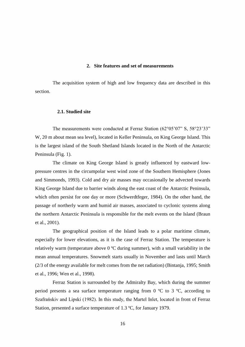
The measurements were conducted at Ferraz Station (62°05’07” S, 58°23’33”

W, 20 m about mean sea level), located in Keller Peninsula, on King George Island. This

is the largest island of the South Shetland Islands located in the North of the Antarctic

Peninsula (Fig. 1).

The climate on King George Island is greatly influenced by eastward low-

pressure centres in the circumpolar west wind zone of the Southern Hemisphere (Jones

and Simmonds, 1993). Cold and dry air masses may occasionally be advected towards

King George Island due to barrier winds along the east coast of the Antarctic Peninsula,

which often persist for one day or more (Schwerdtfeger, 1984). On the other hand, the

passage of northerly warm and humid air masses, associated to cyclonic systems along

the northern Antarctic Peninsula is responsible for the melt events on the Island (Braun

et al., 2001).

The geographical position of the Island leads to a polar maritime climate,

especially for lower elevations, as it is the case of Ferraz Station. The temperature is

relatively warm (temperature above 0 ºC during summer), with a small variability in the

mean annual temperatures. Snowmelt starts usually in November and lasts until March

(2/3 of the energy available for melt comes from the net radiation) (Bintanja, 1995; Smith

et al., 1996; Wen et al., 1998).

Ferraz Station is surrounded by the Admiralty Bay, which during the summer

period presents a sea surface temperature ranging from 0 ºC to 3 ºC, according to

Szafrańskiv and Lipski (1982). In this study, the Martel Inlet, located in front of Ferraz

Station, presented a surface temperature of 1.3 ºC, for January 1979.

17

Figure 1 - Geographical location of Ferraz Station. Adapted from Moura (2009).

Observational field campaigns are difficult to be carried out in this region due to

harsh climatic conditions and the difficult access to the Ferraz Station. As a member of

the observational campaign team I attended, in November 2014 and February 2015, the

process of installation and removal of high frequency equipment.

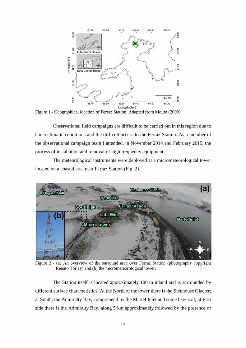
The meteorological instruments were deployed at a micrometeorological tower

located on a coastal area near Ferraz Station (Fig. 2).

Figure 2 - (a) An overview of the surround area over Ferraz Station (photography copyright

Renato Torlay) and (b) the micrometeorological tower.

The Station itself is located approximately 100 m inland and is surrounded by

different surface characteristics. At the North of the tower there is the Stenhouse Glacier;

at South, the Admiralty Bay, comprehend by the Martel Inlet and some bare soil; at East

side there is the Admiralty Bay, along 5 km approximately followed by the presence of

18

another Peninsula with glacier, and at West/Northwest side there is bare soil, usually

covered by snow, represented by hills (maximum height around 330 m) (Junior et al.

2012), as displayed in Figure 2.

The surface where the tower is located consists of rocks and gravels (< 1 m in

width). Near the tower (< 10 m) there is a lake (South Lake), which is often frozen except

in some Summer days. Furthermore, there is no vegetation near the tower excepted in the

Southeast and Northeast where moss grows over a distance > 100 m.

2.2. High frequency measurements on the tower

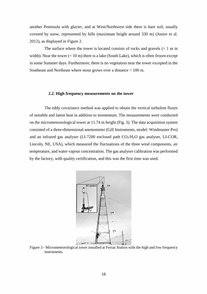
The eddy covariance method was applied to obtain the vertical turbulent fluxes

of sensible and latent heat in addition to momentum. The measurements were conducted

on the micrometeorological tower at 11.74 m height (Fig. 3). The data acquisition system

consisted of a three-dimensional anemometer (Gill Instruments, model: Windmaster Pro)

and an infrared gas analyser (LI-7200 enclosed path CO2/H2O gas analyser, LI-COR,

Lincoln, NE, USA), which measured the fluctuations of the three wind components, air

temperature, and water vapour concentration. The gas analyser calibration was performed

by the factory, with quality certification, and this was the first time was used.

Figure 3 - Micrometeorological tower installed at Ferraz Station with the high and low frequency

instruments.

19

The eddy covariance sampling frequency was 10 Hz and the data were stored at

30 min (average) interval for subsequent flux calculation. For data processing was used

the Software EddyPro - version 5.0 (<https://www.licor.com/>), with corrections for

wind measurements, angle-of-attack correction for wind components (Nakai and

Shimoyanma, 2012) and double rotation for tilt correction. Was used for density

fluctuations, which works as a correction for heat fluxes, the method suggested for Webb

et al. (1980) and Ibrom et al. (2007). Spectral corrections, for low and high frequency

ranges, were applied using the methods suggested for Moncrieff et al. (2004) and

Moncrieff et al. (1997), which is used correction of high and low-pass filtering effects.

Statistical tests for range check and spike check were applied (Vickers and Mahrt, 1997)

removing the trend in 30 min data. Furthermore, questionable data were discard using

criteria for selection data, as discussed for Park et al. (2013) and described in Table 1.

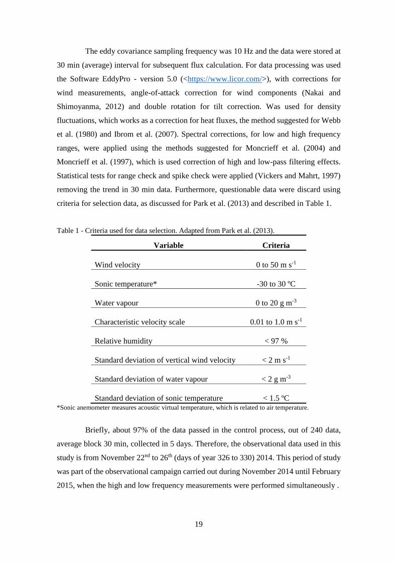
Table 1 - Criteria used for data selection. Adapted from Park et al. (2013).

Variable Criteria

Wind velocity 0 to 50 m s-1

Sonic temperature* -30 to 30 ºC

Water vapour 0 to 20 g m-3

Characteristic velocity scale 0.01 to 1.0 m s-1

Relative humidity < 97 %

Standard deviation of vertical wind velocity < 2 m s-1

Standard deviation of water vapour < 2 g m-3

Standard deviation of sonic temperature < 1.5 ºC *Sonic anemometer measures acoustic virtual temperature, which is related to air temperature.

Briefly, about 97% of the data passed in the control process, out of 240 data,

average block 30 min, collected in 5 days. Therefore, the observational data used in this

study is from November 22nd to 26th (days of year 326 to 330) 2014. This period of study

was part of the observational campaign carried out during November 2014 until February

2015, when the high and low frequency measurements were performed simultaneously .

20

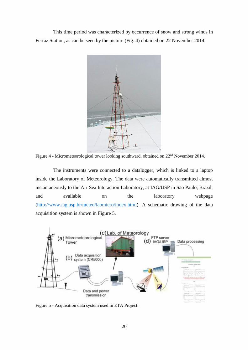
This time period was characterized by occurrence of snow and strong winds in

Ferraz Station, as can be seen by the picture (Fig. 4) obtained on 22 November 2014.

Figure 4 - Micrometeorological tower looking southward, obtained on 22nd November 2014.

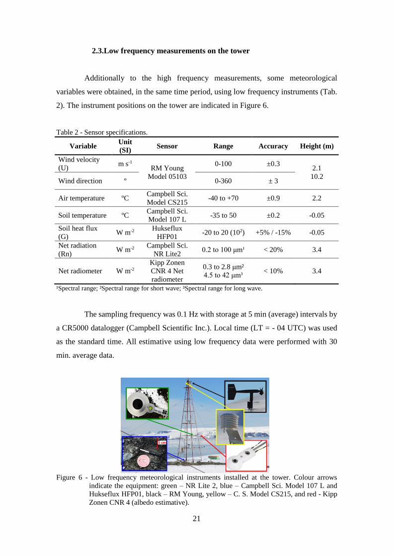
The instruments were connected to a datalogger, which is linked to a laptop

inside the Laboratory of Meteorology. The data were automatically transmitted almost

instantaneously to the Air-Sea Interaction Laboratory, at IAG/USP in São Paulo, Brazil,

and available on the laboratory webpage

(http://www.iag.usp.br/meteo/labmicro/index.html). A schematic drawing of the data

acquisition system is shown in Figure 5.

Figure 5 - Acquisition data system used in ETA Project.

21

2.3.Low frequency measurements on the tower

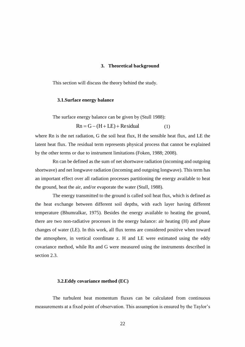
Additionally to the high frequency measurements, some meteorological

variables were obtained, in the same time period, using low frequency instruments (Tab.

2). The instrument positions on the tower are indicated in Figure 6.

Table 2 - Sensor specifications.

Variable Unit

(SI) Sensor Range Accuracy Height (m)

Wind velocity

(U) m s-1

RM Young

Model 05103

0-100 ±0.3 2.1

10.2 Wind direction º 0-360 ± 3

Air temperature ºC Campbell Sci.

Model CS215 -40 to +70 ±0.9 2.2

Soil temperature ºC Campbell Sci.

Model 107 L -35 to 50 ±0.2 -0.05

Soil heat flux

(G) W m-2

Hukseflux

HFP01 -20 to 20 (102) +5% / -15% -0.05

Net radiation

(Rn) W m-2

Campbell Sci.

NR Lite2 0.2 to 100 μm¹ < 20% 3.4

Net radiometer W m-2

Kipp Zonen

CNR 4 Net

radiometer

0.3 to 2.8 μm²

4.5 to 42 μm³ < 10% 3.4

¹Spectral range; ²Spectral range for short wave; ³Spectral range for long wave.

The sampling frequency was 0.1 Hz with storage at 5 min (average) intervals by

a CR5000 datalogger (Campbell Scientific Inc.). Local time (LT = - 04 UTC) was used

as the standard time. All estimative using low frequency data were performed with 30

min. average data.

Figure 6 - Low frequency meteorological instruments installed at the tower. Colour arrows

indicate the equipment: green – NR Lite 2, blue – Campbell Sci. Model 107 L and

Hukseflux HFP01, black – RM Young, yellow – C. S. Model CS215, and red - Kipp

Zonen CNR 4 (albedo estimative).

22

3. Theoretical background

This section will discuss the theory behind the study.

3.1.Surface energy balance

The surface energy balance can be given by (Stull 1988):

sidualRe)LEH(GRn (1)

where Rn is the net radiation, G the soil heat flux, H the sensible heat flux, and LE the

latent heat flux. The residual term represents physical process that cannot be explained

by the other terms or due to instrument limitations (Foken, 1988; 2008).

Rn can be defined as the sum of net shortwave radiation (incoming and outgoing

shortwave) and net longwave radiation (incoming and outgoing longwave). This term has

an important effect over all radiation processes partitioning the energy available to heat

the ground, heat the air, and/or evaporate the water (Stull, 1988).

The energy transmitted to the ground is called soil heat flux, which is defined as

the heat exchange between different soil depths, with each layer having different

temperature (Bhumralkar, 1975). Besides the energy available to heating the ground,

there are two non-radiative processes in the energy balance: air heating (H) and phase

changes of water (LE). In this work, all flux terms are considered positive when toward

the atmosphere, in vertical coordinate z. H and LE were estimated using the eddy

covariance method, while Rn and G were measured using the instruments described in

section 2.3.

3.2.Eddy covariance method (EC)

The turbulent heat momentum fluxes can be calculated from continuous

measurements at a fixed point of observation. This assumption is ensured by the Taylor’s

23

hypothesis about the frozen turbulence (Kaimal and Finnigan, 1994). The turbulent

motions are mathematically described using Reynold’s decomposition, assuming

statistical stationary during the average time. The Reynold’s decomposition can be

written as:

'XXX (2)

in which the instantaneous value of the variable X is the sum of its average value ( X ) in

time and its deviation value (X’) from the average. Thus, the vertical turbulent fluxes are

the covariance between the fluctuations of the vertical wind velocity (w’) and the variable

of interest. These fluxes can be physically understood and mathematically expressed by

the momentum and/or scalar conservation equation. Considering the presence of

atmospheric turbulence, null horizontal advection (e.g. steady-state conditions), and flat

and homogeneous terrain, the turbulent fluxes can be described as (Stull, 1988, Foken et

al., 2012):

''wcH pa (3)

q'w'λLE (4)

where ρa (kg m-3) is the air density, cp (J kg-1 K-1) the air specific heat at constant pressure,

and λ (J kg-1) the latent heat of evaporation. w’, θ’, and q’ are the fluctuations of the wind

vertical component, potential temperature, and specific humidity of air, respectively.

3.3.Vertical turbulent flux of horizontal momentum (τ)

The momentum flux can be estimate using the EC as:

22

a 'v'w'u'w (5)

with u’ and v’ being the fluctuations of the horizontal components of wind (zonal and

meridional).

Another possibility to estimate τ is by using bulk parameterization, which is a

useful tool widely adopted in forecast numerical models to represent the turbulent fluxes

(heat and momentum). This application is especially used in remote areas, (e.g. over the

ocean and in Polar regions), when direct measurements are not commonly feasible

(Cassano et al., 2001; Vickers and Mahrt, 2006; Guo and Zang, 2007; Town and Walden,

2009).

24

The standard bulk formula used in most forecast numerical models using the Cd

can be written as (Vickers and Mahrt, 2006):

2

da UC (6)

where U is the mean wind velocity (m s-1) and Cd is the bulk transfer coefficient for

momentum.

The required Cd shall be estimated, for instance, using the momentum flux

obtained by EC method and wind velocity.

3.4.Atmospheric surface layer stability parameter

The surface layer can be analysed in the context of the Monin-Obukhov

similarity theory, with the turbulent fluxes measured at this layer contributing to provide

parameters that can describe the turbulence structure in the surface layer. Using

Buckingham Pi dimensional analysis method (Perry et al., 1963, apud., Stull, 1988),

similarity relationships, characteristics scales, and atmospheric stability parameter can be

formed through relevant variables (vertical gradient of wind velocity, sensible heat flux,

momentum flux, buoyancy parameter, and measured height) (Monin and Obukhov, 1954;

Bussinger et al., 1971; Wygaard, 1973; Sorbjan, 1986).

The characteristic scales of wind velocity ( *u ) and potential temperature ( * ),

in the surface layer, can be given by:

2

1

a

*u

(7)

*

*u

H (8)

The dimensionless atmospheric stability parameter L)dz( can be

obtained using the measured height (z), the displacement height (d), and the Obukhov

Length:

)''wg41.0(

uL

0

3

*

(9)

25

where g is the Earth’s gravity (considered here as 9.81 m s-2), 0.41 the Von Kármán’s

constant, θ0 (K) the reference temperature (average value), and ''w the covariance

between the fluctuations of vertical component of wind velocity and of potential

temperature. |L| represents the height above the surface where the buoyancy and

mechanical productions of turbulent kinetic energy are of equal magnitude; below this

height, mechanical effect dominates and above it, buoyancy effect dominates (Stull

1988). The ζ signal is basically determined by the signal of ''w .

3.5.Turbulent kinetic energy

The turbulent transport of heat and momentum can be related to the turbulent

kinetic energy (TKE, m2 s-2), which is a useful measure of the turbulence intensity

throughout the surface layer. The TKE is defined as the sum of the wind velocity

component variances ),,( 2

w

2

v

2

u divided by two, as follow:

)(2

1)'w'v'u(

2

1eTKE 2

w

2

v

2

u

222 (10)

The temporal and spatial evolution of TKE in the PBL is determined by the

mechanical production rate (P, m2 s-2), the buoyancy production/destruction (B, m2 s-2),

the divergence of the turbulent flow of TKE and pressure fluctuation, the molecular

diffusion and dissipation (as described in Stull 1988).

The P and B terms are related to the vertical turbulent fluxes and can be written

as:

z

U)uw(P ''

(11)

)w(g

B ''

0

(12)

with ''uw being the covariance between fluctuations of vertical and horizontal wind

velocity components and zU the vertical gradient of wind velocity.

26

4. Results and discussion

The main results are presented and discussed in this chapter.

4.1. Observed data

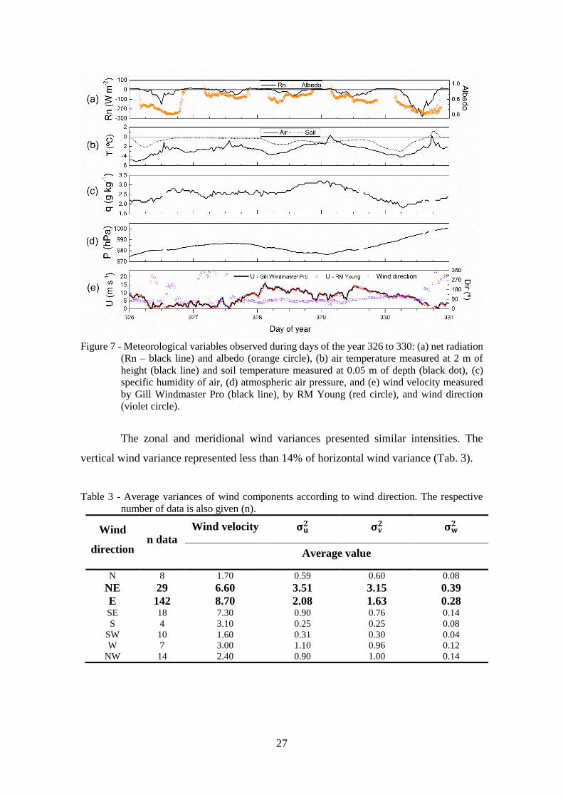
The studied period was characterized by consecutive days with small Rn values

indicating cloudy days (days of the year 326 to 329), and the last investigated day with

comparatively larger values of Rn (Fig.7a). The period of cloudiness was caused by the

influence of low-pressure systems over the region during these days with the presence of

dry snow (albedo ≈ 0.8 - 0.9) found during days with low Rn values and progressive

melting snow (albedo < 0.8 decreasing to 0.6) under relatively clear days, over high-

pressure system (Fig. 7a,d). Raddatz et al. (2015) discuss the relationship between albedo

values and snow presence.

Most of time, the soil temperature, measured at 0.05 m of depth, presented

negative values (Fig. 7b). The air temperature, measured at 2 m of height, was cooler than

the soil temperature, except for short time period as seen on day 329. The small temporal

variation of soil temperature is an indicative of snow cover (Fig. 7b).

The specific humidity of air (q) varied from ~1.8 g kg-1 to ~ 3.2 g kg-1 (Fig.7c)

with the lower values observed during melting days (small albedo, Fig. 7a).

During the investigated period, most of the wind were from the NE-E sector (171

cases; Tab. 3) and hereafter the discussion will be mainly focused in this sector.

Easterly winds (61% of measured data) presented average intensity around 9 m

s-1 (Fig. 7e and Tab. 3). The higher wind intensities were observed from NE-SE region

(Tab. 3), where the Admiralty Bay is located (Fig. 2).

27

Figure 7 - Meteorological variables observed during days of the year 326 to 330: (a) net radiation

(Rn – black line) and albedo (orange circle), (b) air temperature measured at 2 m of

height (black line) and soil temperature measured at 0.05 m of depth (black dot), (c)

specific humidity of air, (d) atmospheric air pressure, and (e) wind velocity measured

by Gill Windmaster Pro (black line), by RM Young (red circle), and wind direction

(violet circle).

The zonal and meridional wind variances presented similar intensities. The

vertical wind variance represented less than 14% of horizontal wind variance (Tab. 3).

Table 3 - Average variances of wind components according to wind direction. The respective

number of data is also given (n).

Wind

direction n data

Wind velocity 𝛔𝐮𝟐 𝛔𝐯

𝟐 𝛔𝐰𝟐

Average value

N 8 1.70 0.59 0.60 0.08

NE 29 6.60 3.51 3.15 0.39

E 142 8.70 2.08 1.63 0.28 SE 18 7.30 0.90 0.76 0.14

S 4 3.10 0.25 0.25 0.08

SW 10 1.60 0.31 0.30 0.04

W 7 3.00 1.10 0.96 0.12

NW 14 2.40 0.90 1.00 0.14

28

4.2. Surface layer characteristic scales and atmospheric stability

The surface layer characteristic scales of wind and temperature (Fig. 8) were

estimated using expressions (7) and (8), respectively. Based on these scales, the Obukhov

length was obtained through expression (9) and thereafter the atmospheric stability

parameter (ζ).

Figure 8 - Temporal variation of (a) wind velocity characteristic scale ( *u ) and (b) potential

temperature characteristic scale (* ).

Högström (1990) studied the terms of the turbulent kinetic energy balance and

other second order moments balance in a surface layer experiment in Lövsta, in Southern

Sweden (59º 50’ N). The study classified a range for near-neutral stability condition in

which moderately unstable and slightly stable situations are usually observed.

Using the near-neutral stability condition defined by Högström (1990) as -0.1 ≤

ζ ≤ 0.1, the atmosphere was near-neutral stability during 60.3 % of the time, while the

remainder conditions were unstable (25.5 %) and stable (14.2 %), as indicated in Fig. 9.

Therefore, during the investigated period, the local atmosphere (coastal area) shows

predominantly characteristics of oceanic regions.

29

Figure 9 - Time series of atmospheric stability parameter (ζ): near-neutral (black point), stable

(blue triangle) and unstable (red triangle) conditions. Horizontal black line indicates ζ

= 0 while grey dot line indicates the range around near-neutral condition.

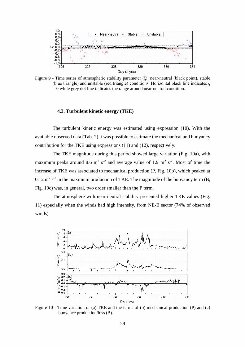
4.3. Turbulent kinetic energy (TKE)

The turbulent kinetic energy was estimated using expression (10). With the

available observed data (Tab. 2) it was possible to estimate the mechanical and buoyancy

contribution for the TKE using expressions (11) and (12), respectively.

The TKE magnitude during this period showed large variation (Fig. 10a), with

maximum peaks around 8.6 m2 s-2 and average value of 1.9 m2 s-2. Most of time the

increase of TKE was associated to mechanical production (P, Fig. 10b), which peaked at

0.12 m2 s-2 in the maximum production of TKE. The magnitude of the buoyancy term (B,

Fig. 10c) was, in general, two order smaller than the P term.

The atmosphere with near-neutral stability presented higher TKE values (Fig.

11) especially when the winds had high intensity, from NE-E sector (74% of observed

winds).

Figure 10 - Time variation of (a) TKE and the terms of (b) mechanical production (P) and (c)

buoyance production/loss (B).

30

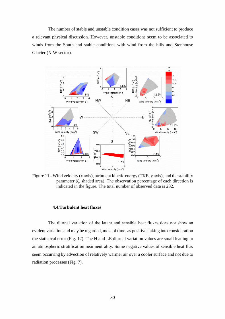
The number of stable and unstable condition cases was not sufficient to produce

a relevant physical discussion. However, unstable conditions seem to be associated to

winds from the South and stable conditions with wind from the hills and Stenhouse

Glacier (N-W sector).

Figure 11 - Wind velocity (x axis), turbulent kinetic energy (TKE, y axis), and the stability

parameter (ζ, shaded area). The observation percentage of each direction is

indicated in the figure. The total number of observed data is 232.

4.4.Turbulent heat fluxes

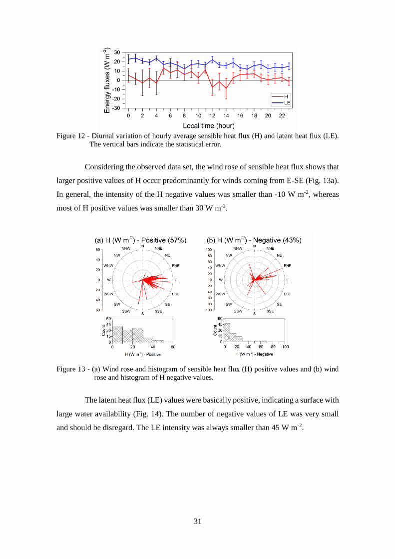
The diurnal variation of the latent and sensible heat fluxes does not show an

evident variation and may be regarded, most of time, as positive, taking into consideration

the statistical error (Fig. 12). The H and LE diurnal variation values are small leading to

an atmospheric stratification near neutrality. Some negative values of sensible heat flux

seem occurring by advection of relatively warmer air over a cooler surface and not due to

radiation processes (Fig. 7).

31

Figure 12 - Diurnal variation of hourly average sensible heat flux (H) and latent heat flux (LE).

The vertical bars indicate the statistical error.

Considering the observed data set, the wind rose of sensible heat flux shows that

larger positive values of H occur predominantly for winds coming from E-SE (Fig. 13a).

In general, the intensity of the H negative values was smaller than -10 W m-2, whereas

most of H positive values was smaller than 30 W m-2.

Figure 13 - (a) Wind rose and histogram of sensible heat flux (H) positive values and (b) wind

rose and histogram of H negative values.

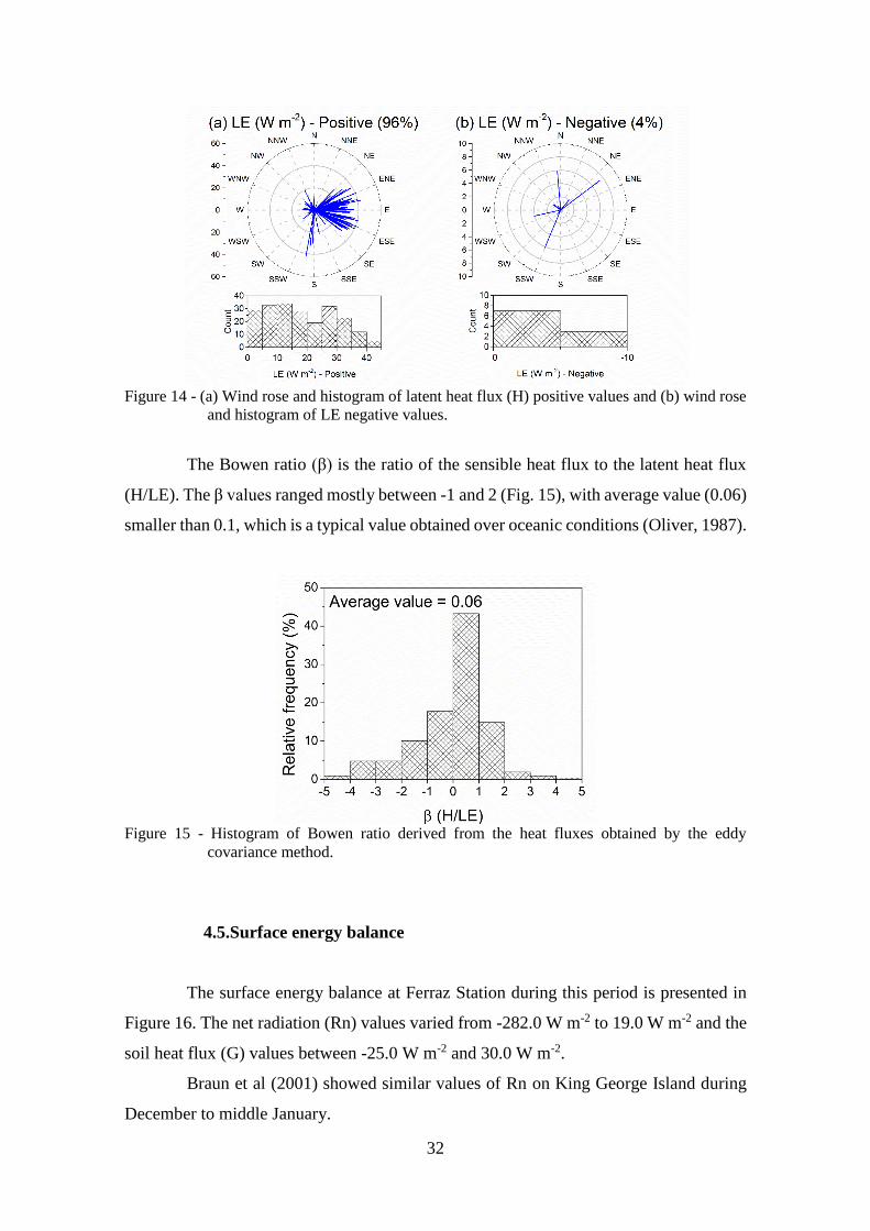
The latent heat flux (LE) values were basically positive, indicating a surface with

large water availability (Fig. 14). The number of negative values of LE was very small

and should be disregard. The LE intensity was always smaller than 45 W m-2.

32

Figure 14 - (a) Wind rose and histogram of latent heat flux (H) positive values and (b) wind rose

and histogram of LE negative values.

The Bowen ratio (β) is the ratio of the sensible heat flux to the latent heat flux

(H/LE). The β values ranged mostly between -1 and 2 (Fig. 15), with average value (0.06)

smaller than 0.1, which is a typical value obtained over oceanic conditions (Oliver, 1987).

Figure 15 - Histogram of Bowen ratio derived from the heat fluxes obtained by the eddy

covariance method.

4.5.Surface energy balance

The surface energy balance at Ferraz Station during this period is presented in

Figure 16. The net radiation (Rn) values varied from -282.0 W m-2 to 19.0 W m-2 and the

soil heat flux (G) values between -25.0 W m-2 and 30.0 W m-2.

Braun et al (2001) showed similar values of Rn on King George Island during

December to middle January.

33

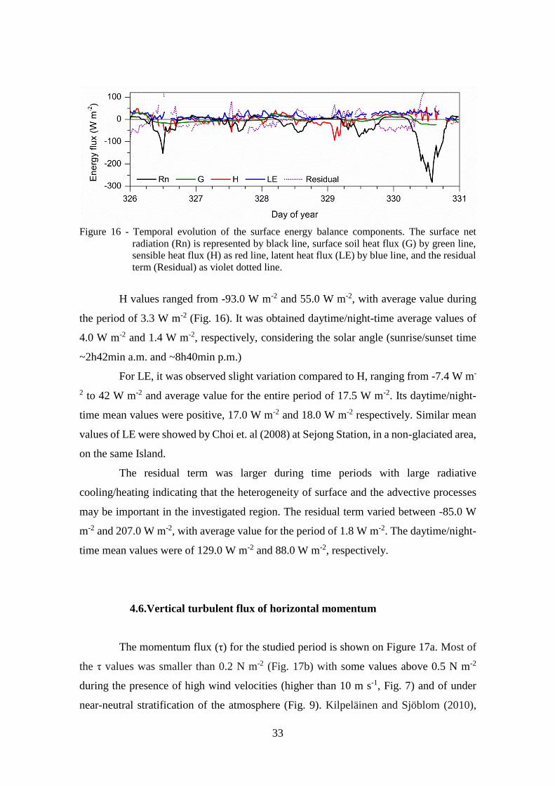
Figure 16 - Temporal evolution of the surface energy balance components. The surface net

radiation (Rn) is represented by black line, surface soil heat flux (G) by green line,

sensible heat flux (H) as red line, latent heat flux (LE) by blue line, and the residual

term (Residual) as violet dotted line.

H values ranged from -93.0 W m-2 and 55.0 W m-2, with average value during

the period of 3.3 W m-2 (Fig. 16). It was obtained daytime/night-time average values of

4.0 W m-2 and 1.4 W m-2, respectively, considering the solar angle (sunrise/sunset time

~2h42min a.m. and ~8h40min p.m.)

For LE, it was observed slight variation compared to H, ranging from -7.4 W m-

2 to 42 W m-2 and average value for the entire period of 17.5 W m-2. Its daytime/night-

time mean values were positive, 17.0 W m-2 and 18.0 W m-2 respectively. Similar mean

values of LE were showed by Choi et. al (2008) at Sejong Station, in a non-glaciated area,

on the same Island.

The residual term was larger during time periods with large radiative

cooling/heating indicating that the heterogeneity of surface and the advective processes

may be important in the investigated region. The residual term varied between -85.0 W

m-2 and 207.0 W m-2, with average value for the period of 1.8 W m-2. The daytime/night-

time mean values were of 129.0 W m-2 and 88.0 W m-2, respectively.

4.6.Vertical turbulent flux of horizontal momentum

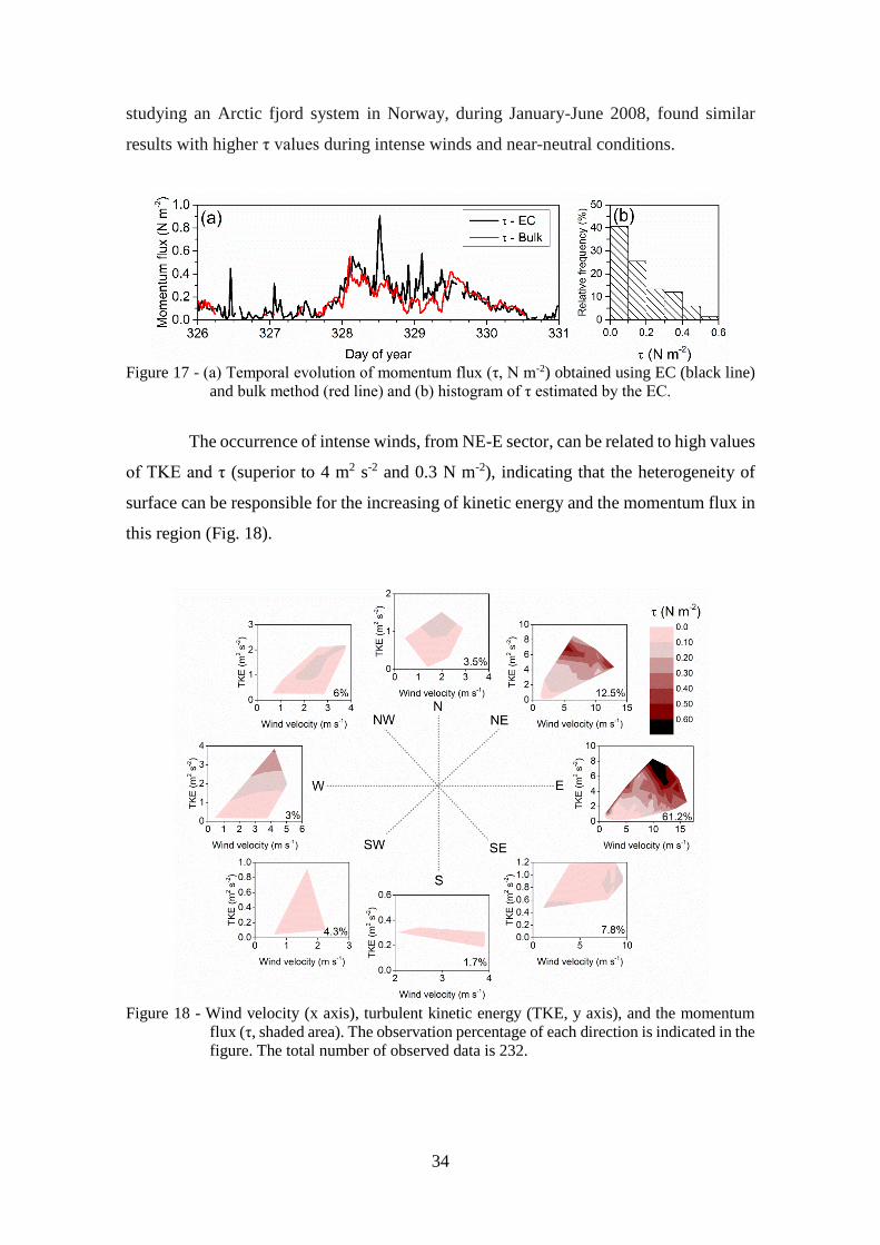
The momentum flux (τ) for the studied period is shown on Figure 17a. Most of

the τ values was smaller than 0.2 N m-2 (Fig. 17b) with some values above 0.5 N m-2

during the presence of high wind velocities (higher than 10 m s-1, Fig. 7) and of under

near-neutral stratification of the atmosphere (Fig. 9). Kilpeläinen and Sjöblom (2010),

34

studying an Arctic fjord system in Norway, during January-June 2008, found similar

results with higher τ values during intense winds and near-neutral conditions.

Figure 17 - (a) Temporal evolution of momentum flux (τ, N m-2) obtained using EC (black line)

and bulk method (red line) and (b) histogram of τ estimated by the EC.

The occurrence of intense winds, from NE-E sector, can be related to high values

of TKE and τ (superior to 4 m2 s-2 and 0.3 N m-2), indicating that the heterogeneity of

surface can be responsible for the increasing of kinetic energy and the momentum flux in

this region (Fig. 18).

Figure 18 - Wind velocity (x axis), turbulent kinetic energy (TKE, y axis), and the momentum

flux (τ, shaded area). The observation percentage of each direction is indicated in the

figure. The total number of observed data is 232.

35

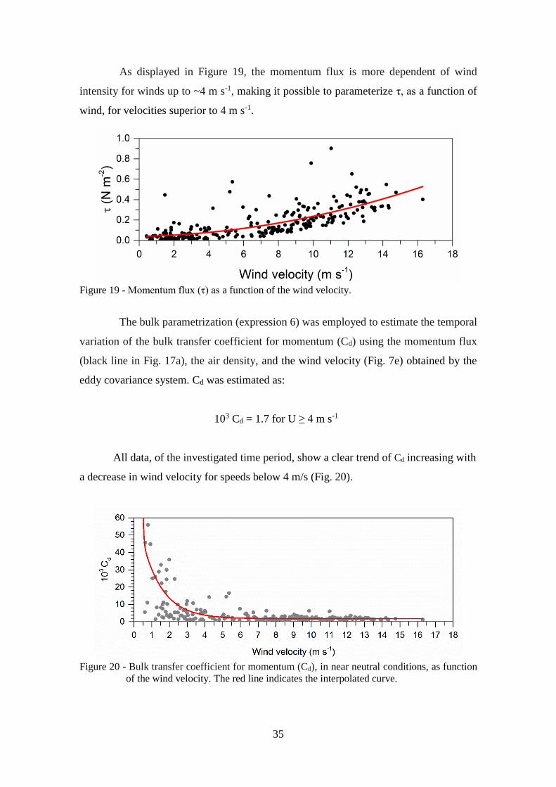
As displayed in Figure 19, the momentum flux is more dependent of wind

intensity for winds up to ~4 m s-1, making it possible to parameterize τ, as a function of

wind, for velocities superior to 4 m s-1.

Figure 19 - Momentum flux (τ) as a function of the wind velocity.

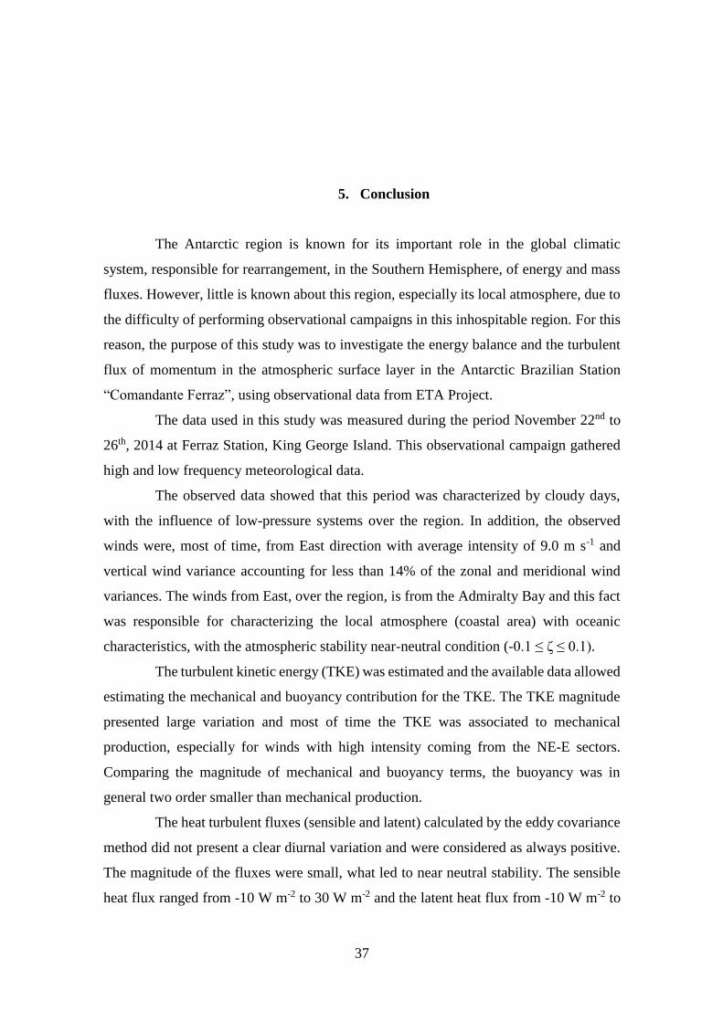
The bulk parametrization (expression 6) was employed to estimate the temporal

variation of the bulk transfer coefficient for momentum (Cd) using the momentum flux

(black line in Fig. 17a), the air density, and the wind velocity (Fig. 7e) obtained by the

eddy covariance system. Cd was estimated as:

103 Cd = 1.7 for U ≥ 4 m s-1

All data, of the investigated time period, show a clear trend of Cd increasing with

a decrease in wind velocity for speeds below 4 m/s (Fig. 20).

Figure 20 - Bulk transfer coefficient for momentum (Cd), in near neutral conditions, as function

of the wind velocity. The red line indicates the interpolated curve.

36

The Cd value found for the investigated time period agree with literature studies

performed in the Antarctic region. Andreas and Claffey (1995) obtained Cd values ranging

from 1.3 x 10-3 to 2.5 x 10-3, for the Ice Station Weddell, using data from February and

March 1992. Lingen et al. (1998) obtained Cd values varying between 0.89 x 10-3 to 2.6

x 10-3 in the East Antarctic region (Chinese station of Zhongshan) during December of

1996.

A temporal variation of the momentum flux (red line of Fig.17a) was calculated,

by expression (6), using the estimated Cd (Fig. 20), an average air density value (1.24 kg

m-3), and the wind velocity data obtained by the low frequency measurement at 10.2 m

height (Fig. 7e).

The statistical comparison between τ calculated by EC and by the Bulk

formulation shows a root mean square error of 0.12 N m-2, an index of agreement of 0.72

and the Pearson’s correlation of 0.6 showing a reasonable agreement between the

momentum flux estimated by different methods.

Figure 21 - Dispersion diagram between τ estimated by EC and by bulk formulation for wind

velocity superior to 4.0 m s-1. The red line indicates the linear interpolation.

37

5. Conclusion

The Antarctic region is known for its important role in the global climatic

system, responsible for rearrangement, in the Southern Hemisphere, of energy and mass

fluxes. However, little is known about this region, especially its local atmosphere, due to

the difficulty of performing observational campaigns in this inhospitable region. For this

reason, the purpose of this study was to investigate the energy balance and the turbulent

flux of momentum in the atmospheric surface layer in the Antarctic Brazilian Station

“Comandante Ferraz”, using observational data from ETA Project.

The data used in this study was measured during the period November 22nd to

26th, 2014 at Ferraz Station, King George Island. This observational campaign gathered

high and low frequency meteorological data.

The observed data showed that this period was characterized by cloudy days,

with the influence of low-pressure systems over the region. In addition, the observed

winds were, most of time, from East direction with average intensity of 9.0 m s-1 and

vertical wind variance accounting for less than 14% of the zonal and meridional wind

variances. The winds from East, over the region, is from the Admiralty Bay and this fact

was responsible for characterizing the local atmosphere (coastal area) with oceanic

characteristics, with the atmospheric stability near-neutral condition (-0.1 ≤ ζ ≤ 0.1).

The turbulent kinetic energy (TKE) was estimated and the available data allowed

estimating the mechanical and buoyancy contribution for the TKE. The TKE magnitude

presented large variation and most of time the TKE was associated to mechanical

production, especially for winds with high intensity coming from the NE-E sectors.

Comparing the magnitude of mechanical and buoyancy terms, the buoyancy was in

general two order smaller than mechanical production.

The heat turbulent fluxes (sensible and latent) calculated by the eddy covariance

method did not present a clear diurnal variation and were considered as always positive.

The magnitude of the fluxes were small, what led to near neutral stability. The sensible

heat flux ranged from -10 W m-2 to 30 W m-2 and the latent heat flux from -10 W m-2 to

38

45 W m-2. Bowen ratio ranged from -5 to 5, with average value of 0.06, which is a typical

value for oceanic conditions.

Considering the heat turbulent fluxes calculated and the net radiation and soil

heat flux measured directly, it was possible to present the energy balance for this period.

The temporal variation of the latent heat flux showed slight variation compared to the

sensible heat flux, with the respective daytime/night-time values of 17/18 W m-2 and 4/1.4

W m-2. The residual term was large in this period, especially in the presence of large

radiative cooling/heating suggesting that the surface heterogeneity and advective process

are relevant to this region.

The vertical turbulent flux of horizontal momentum (τ) was estimated using the

eddy covariance measurements. Most of its values was smaller than 0.2 N m-2 with higher

peaks that could be associated to high wind velocities during atmosphere under near-

neutral stratification. Also, it was verified that the momentum flux is dependent on wind

velocity, for velocity intensity higher than between τ calculated by EC and by the Bulk

formulation 4.0 m s-1.

The bulk transfer coefficient for momentum flux (Cd) obtained in this work was

of 1.7 x 10-3, which agrees with previous work performed in the Antarctic region.

A temporal variation of the momentum flux was also calculated using the Cd

estimated and the wind velocity data obtained by the low frequency measurement at 10.2

m height. A statistical comparison between the momentum fluxes calculated by eddy

covariance method and by bulk formulation showed reasonable agreement.

Future works

It is suggested as future work to:

- To perform a spectral analysis of the turbulent data;

- To estimate the bulk transfer coefficients of momentum and heat using different

approaches;

- To estimate the footprint of the turbulent fluxes;

- To estimate indirectly the turbulent fluxes using different techniques and to

compare with the fluxes obtained by eddy covariance.

39

References

Andreas E.L., Claffey K.J.: 1995. Air-ice drag coefficients in the western Weddell Sea:

1. Values deduced from profile measurements. Journal of Geophysical Research,

100(C3), 4821-4831, doi:10.1029/94JC02015.

Argentini S., Mastrantonio G., Viola A.: 1999. Estimation of turbulent heat fluxes and

exchange coefficients for heat at Dumont d’Urville, East Antarctica. Antarctic Science,

11 (1), 93-99.

Aubinet M., Vesala T., Papale D.: 2012. Eddy Covariance: A Practical Guide to

Measurement and Data Analysis, Springer, London, UK.

Bhumralkar C. M.: 1975. Numerical Experiments on the Computation of Ground Surface

Temperature in an Atmospheric General Circulation. Model. Journal Applied

Meteorology, 14, 1246–1258. DOI: http://dx.doi.org/10.1175/1520-

0450(1975)014<1246:NEOTCO>2.0.CO;2

Bintanja R.: 1995. The local surface energy balance of the Ecology Glacier, King George

Island, Antarctica: measurements and modelling. Antarctic Science, 7, 315–325.

Braun M., Saurer H., Vogt S., Simões J.C., Goßmann H.: 2001. The influence of large-

scale atmospheric circulation on the surface energy balance of the King George Island ice

cap. Int. J. Climatol., 21, 21–36. DOI: 10.1002/joc.563.

Bussinger J. A., Wyngaard J. C., Izumi Y., Bradley E. F.: 1971. Flux-Profile

Relationships in the Atmospheric Surface Layer. J. Atmos. Sciences. 28, 181-189.

Cassano J. J., Parish T. R., King J. C.: 2001. Evaluation of the Turbulent Surface Flux

Parameterizations for the Stable Surface Layer over Halley, Antarctica. Monthly Weather

Review. 129, 26-46.

Chen X. Y., Tung K. K.: 2014. Varying planetary heat sink led to global-warming

slowdown and acceleration, Science, 345, 897–903, doi:10.1126/science.1254937.

Choi T., Lee, B. Y., Lee, H. C., Shim, J. S.: 2004. Surface flux measurements at King

Sejong Station in West Antarctica. I. Turbulent characteristics and sensible heat flux.

Ocean and Polar Research, 26, 453–463.

Choi T., Lee B. Y., Kim S-J, Yoon Y. J., Lee H-C.:2008. Net radiation and turbulent

energy exchanges over a non-glaciated coastal area on King George Island during four

summer seasons. Antarctic Science. 20, 1, 99-111.

Doran P. T., McKay C. P., Clow G. D., Dana G. L., Fountain A. G., Nylen T., Lyons W.

B.: 2002. Valley floor climate observations from the McMurdo dry valleys, Antarctica,

40

1986-2000. Journal of Geophysical Research, 107 (D24) :4772,

doi:10.1029/2001JD002045.

Foken, T.: 1998. Die scheinbar ungeschlossene Energiebilanz am Erdboden—eine

Herausforderung an die Experimentelle Meteorologie. Sitzungsberichte der Leibniz-

Sozieta. 24, 131–150.

Foken T.: 2008. The energy balance closure problem: An overview. Ecological

Applications 18:1351–1367.http://dx.doi.org/10.1890/06-0922.1

Foken T., Aubinet M., Leuning R.: 2012. The eddy covariance method. In: Eddy

Covariance: A Practical Guide to Measurements and Data Analysis (eds. M. Aubinet, M.

Vesala, T. Papale). Springer Atmospheric Sciences, Netherlands, pp.1-19. DOI:

10.1007/978-94-007-2351-1.

Garrat J. R.:1992. The atmospheric boundary layer. Cambridge University Press,

Cambridge, 316 pp.

Guo X. and Zhang H.: 2007. A performance comparison between nonlinear similarity

functions in bulk parameterization for very stable conditions. Environ Fluid Mech., 7,

239-257.

Hines K. M., Grumbine R. W., Bromwich D. H., Cullather R. I.: 1999. Surface energy

balance of the NCEP MRF and NCEP– NCAR reanalysis in Antarctic latitudes during

FROST. Weather Forecasting. 14, 851–866.

Högström U.: 1990. Analysis of turbulence structure in the surface layer with a modified

similarity formulation for near neutral conditions. J. Atmos. Sci. 47: 1949-1972, doi:

http://dx.doi.org/10.1175/1520-0469(1990)047<1949:AOTSIT>2.0.CO;2

Ibrom, A., Dellwik E., S Larse. E., Pilegaard K..: 2007. On the use of the Webb-Pearman-

Leuning theory for closed-path eddy correlation measurements, Tellus Series B-Chemical

and Physical Meteorology, 59:937-946.

Jones D. A, Simmonds I. H.: 1993. A climatology of southern hemisphere extratropical

cyclones. Clim Dyn 9, 131–145. DOI: 10.1007/BF00209750.

Junior M., Dani C. W., Arigony-Neto N., Simoes J., Simões J. C., Velho L. F., Ribeiro

R. R., Parnow I., Bremer U. F., Júnior E. S. F., Erwes H. J. B.: 2012. A new topographic

map for Keller Peninsula, King George Island, Antarctica. Pesquisa Antártica Brasileira,

5, 105-113.

Kaimal, J. C., and J. J. Finnigan.: 1994. Atmospheric Boundary Layer Flows - Their

structure and measurement. Oxford University Press, 289 pp.

Kilpeläinen T. and Sjöblom A.: 2010. Momentum and Sensible Heat Exchange in an

Ice-Free Arctic Fjord. Boundary-Layer Meteorol,134:109–130, doi: 10.1007/s10546-

009-9435-x.

King J. C. and Anderson P. S.: 1994. Heat and water vapour fluxes and scalar roughness

lengths over an Antarctic ice shelf. Boundary-Layer Meteorol, 69, 101-121.

41

King J. C, Connolley W. M.: 1997. Validation of the surface energy balance over the

Antarctic ice sheets in the U.K. Meteorological Office unified climate model. Journal of

Climate. 10, 1273–1287. ,

King J. C., Argentini S. A., Anderson P. S.: 2006. Contrast between the summertime

surface energy balance and boundary layer structure at Dome C and Halley stations,

Antarctica. Journal of Geophysical Research, 111, 1-13.

King J. C., Gardia A., Kirchgaessner A., Munneke P. K., Lachlan-Cope T. A., Orr A.,

Reijmer C., Van den Broeke M. R., Van Wessem J. M., Weeks M.: 2015. Validation of

the summertime surface energy budget of Larsen C Ice Shelf (Antarctica) as represented

in three high-resolution atmospheric models. Journal of Geophysical Research. 120,

1335-1347.

Lingen B., Longhua L., Pengqun J.: 1998. Experimental observation on the characteristics

of the near-surface turbulence over the Antarctic ice sheets during the polar day period.

Science in China (Series D), 41 (3), 262-268.

Moncrieff, J. B., Massheder J. M., de Bruin H., Ebers J., Friborg T., Heusinkveld B.,

Kabat P., Scott S., Soegaard H., Verhoef A.: 1997. A system to measure surface fluxes

of momentum, sensible heat, water vapor and carbon dioxide. Journal of Hydrology, 188-

189: 589-611.

Moncrieff, J. B., Clement R., Finnigan J., Meyers T.: 2004. Averaging, detrending and

filtering of eddy covariance time series, in Handbook of micrometeorology: a guide for

surface flux measurements, eds. Lee, X., Massman W. J., Law B. E.. Dordrecht: Kluwer

Academic, 7-31.

Monin A. S. and Obukhov A. M.: 1954. Basic laws of turbulent mixing in the atmosphere

near the ground. Tr. Akad. Nauk. SSSR Geophiz. Inst. 24: 151, 1963-1987.

Montgomery R. B.: 1948. Vertical eddy flux of heat in the atmosphere. Journal of

Meteorology. 5, 265-274.

Moura R.B.: 2009. Estudo taxonômico dos Holothuroidea (Echinodermata) das Ilhas

Shetland do Sul e do Estreito de Bransfield, Antártica. Master Dissertation, Museu

Nacional, Universidade Federal do Rio de Janeiro, Rio de Janeiro, 111 pp

Nakai, T., Shimoyama K.: 2012. Ultrasonic anemometer angle of attack errors under

turbulent conditions. Agricultural and Forest Meteorology, 18: 162-163.

Obukhov, A. M.: 1951. Charakteristik mikrostruktury vetra v prizemnom sloje atmosfery

(Characteristics of the micro-structure of the wind in the surface layer in the atmosphere).

Izv AN ASSR ser Geofiz, 3, 49-68.

Oliver, J. E.: 1987. Bowen ratio. Springer US, 183-184 pp. DOI: 10.1007/0-387-30749-

4_30.

Oncley S. P., Friehe C. A., Larue J. C., Businger J. A., Itsweire E. C., Chang S. S.: 1996.

Surface-Layer Fluxes, Profiles, and Turbulence Measurements over Uniform Terrain

under Near-Neutral Conditions. Journal of the Atmospheric Sciences. 53, 7, 1029-1044.

42

Ou N. S., Lin Y.H., Bi X. Q.: 2015. Simulated Heat Sink in the Southern Ocean and Its

Contribution to the Recent Hiatus Decade, Atmospheric and Oceanic Science Letters, 8:3,

174-178.

Panin G. N., Tetzlaff G., Raabe A.: 1998. Inhomogeneity of the land surface and problems

in the parameterization of surface fluxes in natural conditions. Theoretical and Applied

Climatology 60:163–178.

Park S-J., Choi T-J., and Kim S-J.: 2013. Heat flux variations over sea ice observed at the

coastal area of the Sejong Station, Antarctica. Asia-Pacific Journal Atmospheric, 49, 4,

443-450.

Raddatz R. L., Papakyriakou T. N., Else B. G., Swystun K., Barber D. G.: 2015. A simple

scheme for estimating turbulent heat flux over landfast artic sea ice from dry snow to

advanced melt. Boundary-Layer Meteorol, 155, 351-367. DOI 10.1007/s10546-014-

0002-8.

Schneider, C.: 1999. Energy balance estimates during the summer season of glaciers of

the Antarctic Peninsula. Global and Planetary Change, 22, 117–130.

Schwerdtfeger W.:1984. Weather and Climate of the Antarctic. Elsevier, Amsterdam.

262p.

Smith, R. C., Stammerjohn, S. E. and Baker, K. S.:1996. Surface Air Temperature

Variations in the Western Antarctic Peninsula Region. In: Foundations for Ecological

Research West of the Antarctic Peninsula (eds R. M. Ross, E. E. Hofmann and L. B.

Quetin), American Geophysical Union, Washington, D. C.. doi: 10.1029/AR070p0105.

Sorbjan Z.: 1986. On similarity in the atmospheric boundary layer. Bound Layer Meteor.,

34, 377-397.

Stull, R. B.: 1988. An introduction to boundary layer meteorology. Kluwer Academic

Press, Dordrecht 666pp.

Swinbank W. C.: 1951. The measurement of vertical transfer of heat and water vapour by

eddies in the lower atmosphere. Journal of Meteorology. 8, 135-145.

Szafrański Z. and Lipski M.: 1982. Characteristics of water temperature and salinity at

Admiralty Bay (King George Island, South Shetland Islands, Antarctic) during the austral

summer 1978/79. Pol. Polar Res., 3 (1-2), 7-24.

Targett P. S.: 1998. Katabatic winds, hydraulic jumps and wind flow over the Vestfold

Hills, East Antarctica. Antarctica Science, 10(4) :502-506.

Town M. S. and Walden V. P.: 2009. Surface energy budget over the South Pole and

turbulent heat fluxes as a function of an empirical bulk Richardson number. Journal of

Geophysical Research, 114, D22107, DOI: 10.1029/2009JD011888.

Turner J., Marshall G. J., and Lachlan-Cope T.: 1998. Analysis of synoptic-scale low

pressure systems within the Antarctic Peninsula sector of the circumpolar trough.

International Journal of Climatology, 18, 253–280.

43

Van As D., Van Den Broeke M., Reijmer C., and Van De Wal R.: 2005. The summer

surface energy balance of the high Antarctic Plateau. Boundary-Layer Meteorology, 115,

289–317.

Van Den Broeke M., Reijmer C., Van As D., Van de Wal, and Oerlemans J.: 2005.

Seasonal cycles of Antarctic surface energy balance from automatic weather stations.

Annals of Glaciology, 41. 131-139.

Vickers, D. and Mahrt L.: 1997. Quality control and flux sampling problems for tower

and aircraft data. Journal of Atmospheric and Oceanic Technology, 14: 512-526.

Vickers, D. and Mahrt L.: 2006. Evaluation of the air-sea bulk formula and sea-surface

temperature variability from observations. Journal of Geophysical Research, 111,

C05002, DOI:10.1029/2005JC003323.

Webb, E. K., Pearman G. I., Leuning R.: 1980. Correction of flux measurements for

density effects due to heat and water vapor transfer. Quarterly Journal of the Royal

Meteorological Society, 106: 85–100.

Wen J., Kang J., Han J., Xie Z., Liu L., Wang D.: 1998. Glaciological studies on King

George Island ice cap, South Shetland Islands, Antarctica. Annals of Glaciology 27:105–

109.

Wyngaard J. C.: 1973. On surface layer turbulence. Workshop on Micrometeorology.

(Ed. D. A. Haugen). Am. Meteor. Soc. 101-148.

Yagüe C., Cano J. L.: 1994. The influence of stratification on the heat and momentum

turbulent transfer in Antarctica. Boundary-Layer Meteorology. 69, 123-136.

Yagüe C., Maqueda G., Rees J. M.: 2003. Characteristics of turbulence in the lower

atmosphere at Halley IV station, Antarctica. Dynamics of Atmosphere and Oceans, 34,

205-223.