Multi Varia Da 1

8/11/2019 Multi Varia Da 1

http://slidepdf.com/reader/full/multi-varia-da-1 1/59

3. The Multivariate Normal Distribution

3.1 Introduction

• A generalization of the familiar bell shaped normal density to severaldimensions plays a fundamental role in multivariate analysis

• While real data are never exactly multivariate normal, the normal densityis often a useful approximation to the “true” population distribution becauseof a central limit effect.

• One advantage of the multivariate normal distribution stems from the fact

that it is mathematically tractable and “nice” results can be obtained.

1



To summarize, many real-world problems fall naturally within the frameworkof normal theory. The importance of the normal distribution rests on its dualrole as both population model for certain natural phenomena and approximatesampling distribution for many statistics.

2



3.2 The Multivariate Normal density and Its Properties

• Recall that the univariate normal distribution, with mean µ and variance σ2,has the probability density function

f (x) = 1√

2πσ2e−[(x−µ)/σ]2/2 − ∞ < x < ∞

• The term x − µ

σ

2

= (x − µ)(σ2)−1(x − µ)

• This can be generalized for p × 1 vector x of observations on serval variablesas

(x − µ)Σ−1(x − µ)

The p × 1 vector µ represents the expected value of the random vector X ,and the p × p matrix Σ is the variance-covariance matrix of X .

3



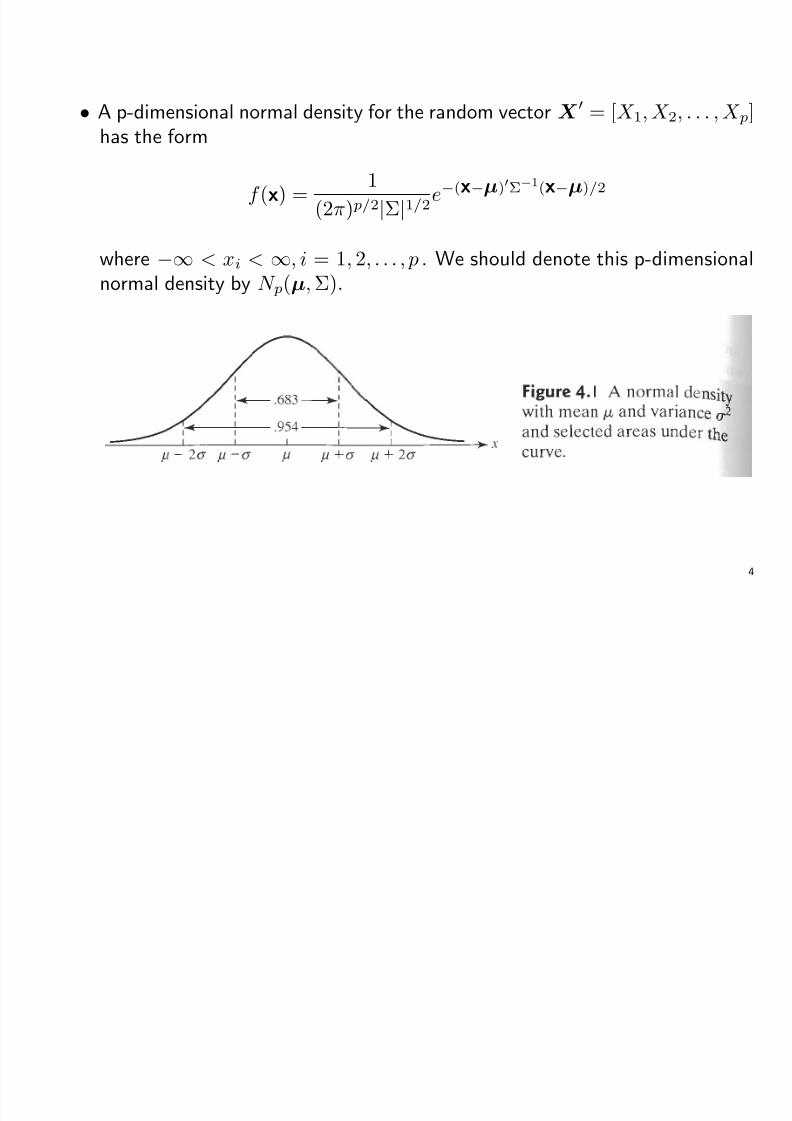
• A p-dimensional normal density for the random vector X = [X 1, X 2, . . . , X p]

has the form

f (x) = 1

(2π) p/2|Σ|1/2e−(x−µ)Σ−1(x−µ)/2

where

−∞ < xi <

∞, i = 1, 2, . . . , p . We should denote this p-dimensional

normal density by N p(µ, Σ).

4



Example 3.1 (Bivariate normal density) Let us evaluate the p = 2 variatenormal density in terms of the individual parameters µ1 = E(X 1), µ2 =E(X

2), σ

11 = Var(X

1), σ

22 = Var(X

2), and ρ

12 = σ

12/(

√ σ11√

σ22

) =Corr(X 1, X 2).

Result 3.1 If Σ is positive definite, so that Σ−1 exists, then

Σe = λe implies Σ−1e = 1

λ

e

so (λ, e) is an eigenvalue-eigenvector pair for Σ corresponding to the pair(1/λ, e) for Σ−1. Also Σ−1 is positive definite.

5



6





Example 4.2 (Contours of the bivariate normal density) Obtain the axesof constant probability density contours for a bivariate normal distribution whenσ11

= σ22

8



The solid ellipsoid of x values satisfying

(x − µ)

Σ

−1

(x − µ) ≤ χ

2

p(α)

has probability 1−α where χ2 p(α) is the upper (100α)th percentile of a chi-square

distribution with p degrees of freedom.

9



Additional Properties of the Multivariate NormalDistribution

The following are true for a normal vector X having a multivariate normaldistribution:

1. Linear combination of the components of X are normally distributed.

2. All subsets of the components of X have a (multivariate) normal distribution.

3. Zero covariance implies that the corresponding components are independentlydistributed.

4. The conditional distributions of the components are normal.

10



Result 3.2 If X is distributed as N p(µ, Σ), then any linear combination of variables aX = a1X 1 + a2X 2 + · · ·+ a pX p is distributed as N (aµ, aΣa). Alsoif aX is distributed as N (aµ, aΣa) for every a, then X must be N p(µ, Σ).

Example 3.3 (The distribution of a linear combination of the componentof a normal random vector) Consider the linear combination aX of amultivariate normal random vector determined by the choice a = [1, 0, . . . , 0].

Result 3.3 If X is distributed as N p(µ, Σ), the q linear combinations

A(q× p)X p×1 =

a11X 1 + · · · + a1 pX pa21X 1 + · · · + a2 pX p

...aq1X 1 +

· · ·+ aqpX p

are distributed as N q(Aµ,AΣA). Also X p×1 + d p×1, where d is a vector of constants, is distributed as N p(µ + d, Σ).

11



Example 3.4 (The distribution of two linear combinations of thecomponents of a normal random vector) For X distributed as N 3(µ, Σ),find the distribution of

X 1 − X 2X 2 − X 3

=

1 −1 00 1 −1

X 1X 2X 3

= AX

12



Result 3.4 All subsets of X are normally distributed. If we respectively partitionX , its mean vector µ, and its covariance matrix Σ as

X ( p×1) =

X 1(q × 1)· · · · · ·

X 2( p − q ) × 1

µ( p×1) =

µ1

(q × 1)· · · · · ·µ2

( p − q ) × 1

and

Σ( p× p) =

Σ11 Σ12

(q × 1) (q × ( p − q ))· · · · · · · · · · · ·

Σ21 Σ22

(( p − q ) × q ) (( p − q ) × ( p − q ))

then X 1 is distributed as N q(µ1, Σ11).

Example 3.5 (The distribution of a subset of a normal random vector)If X is distributed as N 5(µ, Σ), find the distribution of [X 2, X 4].

13



Result 3.5

(a) If X 1 and X 2 are independent, then Cov(X 1,X 2) = 0, a q 1 × q 2 matrix of zeros, where X 1 is q 1 × 1 random vector and X 2 is q 2 × 1. random vector

(b) If

X 1X 2

is N q1+q2

µ1

µ2

,

Σ11 Σ12

Σ21 Σ22

, then X 1 and X 2 are

independent if and only if Σ12 = Σ21 = 0.

(c) If X 1 and X 2 are independent and are distributed as N q1(µ1, Σ11)

and N q2(µ2, Σ22), respectively, then

X 1X 2

has the multivariate normal

distribution

N q1+q2 µ1

µ2

, Σ11 0

0 Σ22

14





Example 3.7 (The conditional density of a bivariate normal distribution)Obtain the conditional density of X 1, give that X 2 = x2 for any bivariatedistribution.

Result 3.7 Let X be distributed as N p(µ, Σ) with |Σ| > 0. Then

(a) (X − µ)Σ−1(X − µ) is distributed as χ2 p, where χ2

p denotes the chi-squaredistribution with p degrees of freedom.

(b) The N p(µ, Σ)distribution assign probability 1 − α to the solid ellipsoid{x : (x −µ)Σ−1(x −µ) ≤ χ2

p(α)}, where χ2 p(α) denote the upper (100α)th

percentile of the χ2 p distribution.

16



Result 3.8 Let X 1,X 2, . . . ,X n be mutually independent with X j distributedas N p(µj, Σ). (Note that each X j has the same covariance matrix Σ.) Then

V1 = c1X 1 + c2X 2 + · · · + cnX n

is distributed as N p

nj=1

cjµj, (n

j=1c2j)Σ

. Moreover, V1 and V2 = b1X 1 +

b2X 2 +· · ·

+ bnX n are jointly multivariate normal with covariance matrix

(n

j=1

c2j)Σ bcΣ

bcΣ21 (

n

j=1

b2j)Σ

Consequently, V 1 and V 2 are independent if bc =n

j=1

cjbj = 0.

17



Example 3.8 (Linear combinations of random vectors) Let X 1,X 2,X 3and X 4 be independent and identically distributed 3 × 1 random vectors with

µ =

3

−11

and Σ =

3 −1 1

−1 1 01 0 2

(a) find the mean and variance of the linear combination aX 1 of the three

components of X 1 where a = [a1 a2 a3].

(b) Consider two linear combinations of random vectors

1

2

X 1 + 1

2

X 2 + 1

2

X 3 + 1

2

X 4

andX 1 + X 2 + X 3 − 3X 4.

Find the mean vector and covariance matrix for each linear combination of vectors and also the covariance between them.

18



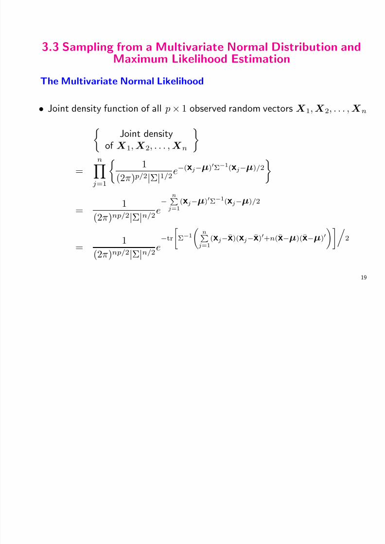
3.3 Sampling from a Multivariate Normal Distribution andMaximum Likelihood Estimation

The Multivariate Normal Likelihood

• Joint density function of all p × 1 observed random vectors X 1,X 2, . . . ,X n

Joint density

of X 1,X 2, . . . ,X n

=

nj=1

1

(2π) p/2|Σ|1/2e−(xj−µ)Σ−1(xj−µ)/2

= 1(2π)np/2|Σ|n/2e

−

nPj=1(xj−µ)

Σ−1

(xj−µ)/2

= 1

(2π)np/2|Σ|n/2e−tr

"Σ−1

nPj=1

(xj−x)(xj−x)+n(x−µ)(x−µ)

!#2

19



• Likelihood

When the numerical values of the observations become available, they maybe substituted for the xj in the equation above. The resulting expression,now considered as a function of µ and Σ for the fixed set of observationsx1, x2, . . . , xn, is called the likelihood .

• Maximum likelihood estimation

One meaning of best is to select the parameter values that maximizethe joint density evaluated at the observations. This technique is calledmaximum likelihood estimation, and the maximizing parameter values arecalled maximum likelihood estimates.

Result 3.9 Let A be a k × k symmetric matrix and x be a k × 1 vector. Then

(a) xAx = tr(xAx) = tr(Axx)

(b) tr(A) =n

i=1

λi, where the λi are the eigenvalues of A.

20



Maximum Likelihood Estimate of µ and Σ

Result 3.10 Given a p × p symmetric positive definite matrix B and a scalarb > 0, it follows that

1

|Σ|be−tr(Σ−1B)/2 ≤ 1

|B|b(2b) pbe−bp

for all positive definite Σ p× p, with equality holding only for Σ = (1/2b)B.

Result 3.11 Let X 1,X 2, . . . ,X n be a random sample from a normal populationwith mean µ and covariance Σ. Then

µ = X and Σ = 1n

nj=1

(X j − X )(X j − X ) = n − 1n S

are the maximum likelihood estimators of µ and Σ, respectively. Their

observed value x and (1/n)n

j=1

(xj

−x)(xj

−x), are called the maximum

likelihood estimates of µ and Σ. 21



Invariance Property of Maximum likelihood estimators

Let θ be the maximum likelihood estimator of θ, and consider the parameter

h(θ), which is a function of θ. Then the maximum likelihood estimate of

h(θ) is given by h(θ).

For example

1. The maximum likelihood estimator of µΣ−1µ is µΣ−1µ, where µ = X andΣ = n−1

n S are the maximum likelihood estimators of µ and Σ respectively.

2. The maximum likelihood estimator of √ σii is

√ σii, where

σii = 1

n

nj=1

(X ij − X i)2

is the maximum likelihood estimator of σii = Var(X i). 22





3.4 The Sampling Distribution of X and S

• The univariate case ( p = 1)

– X is normal with mean µ =(population mean) and variance

1

n

σ2 = population variance

sample size

– For the sample variance, recall that (n−1)s2 =n

j=1(X j− X )2 is distributed

as σ2 times a chi-square variable having n − 1 degrees of freedom (d.f.).– The chi-square is the distribution of a sum squares of independent standard

normal random variables. That is, (n − 1)s2 is distributed as σ2(Z 21 +· · · + Z 2n−1) = (σZ 1)2 + · · · + (σZ n−1)2. The individual terms σZ i areindependently distributed as N (0, σ2).

24



• Wishart distribution

W m(·|Σ) = Wishart distribution with m d.f.

= distribution of n

j=1

ZjZ

j

where Zj are each independently distributed as N p(0, Σ).

• Properties of the Wishart Distribution

1. If A1 is distributed as W m1(A1|Σ) independently of A2, which isdistributed as W m

2

(A2

|Σ), then A1 +A2 is distributed as W m

1+m

2

(A1 +A2|Σ). That is, the the degree of freedom add.

2. If A is distributed as W m(A|Σ), then CAC is distributed asW m(CAC|CΣC).

25



• The Sampling Distribution of X and S

Let X 1,X 2, . . . ,X n be a random sample size n from a p-variate normaldistribution with mean µ and covariance matrix Σ. Then

1. X is distributed as N p(µ, 1nΣ).2. (n − 1)S is distributed as a Wishart random matrix with n − 1 d.f.3. X and S are independent.

26



4.5 Large-Sample Behavior of X and S

Result 3.12 (Law of Large numbers) Let Y 1, Y 2, . . . , Y n be independentobservations from a population with mean E(Y i) = µ, then

Y = Y 1 + Y 2 + · · · + Y n

n

converges in probability to µ as n increases without bound. That is, for anyprescribed accuracy ε > 0, P [−ε < Y − µ < ε] approaches unity as n → ∞.

Result 3.13 (The central limit theorem) Let X 1,X 2, . . . ,X n be independentobservations from any population with mean µ and finite covariance Σ. Then

√ n( X − µ) has an approximate N p(0, Σ)distribution

for large sample sizes. Here n should also be large relative to p.

27



Large-Sample Behavior of X and S

Let X 1,X 2, . . . ,X n be independent observations from a population with mean

µ and finite (nonsingular) covariance Σ. Then

√ n( X − µ)is approximately N p(0, Σ)

and

n( X − µ)

S−1

( X − µ) is approximately χ2 p

for n − p large.

28



3.6 Assessing the Assumption of Normality

• Most of the statistical techniques discussed assume that each vectorobservation X j comes from a multivariate normal distribution.

• In situations where the sample size is large and the techniques dependentsolely on the behavior of X , or distances involve X of the form n( X

−µ)S( X − µ), the assumption of normality for the individual observations isless crucial.

• But to some degree, the quality of inferences made by these methodsdepends on how closely the true parent population resembles the multivariate

normal form.

29



Therefore, we address these questions:

1. Do the marginal distributions of the elements of X

appear to be normal ?What about a few linear combinations of the components X j ?

2. Do the scatter plots of observations on different characteristics give theelliptical appearance expected from normal population ?

3. Are there any “wild” observations that should be checked for accuracy ?

30



Evaluating the Normality of the Univariate MarginalDistributions

• Dot diagrams for smaller n and histogram for n > 25 or so help revealsituations where one tail of a univariate distribution is much longer thanother.

• If the histogram for a variable X i appears reasonably symmetric , we cancheck further by counting the number of observations in certain interval, forexamplesA univariate normal distribution assigns probability 0.683 to the interval

(µi

−

√ σii, µi +

√ σii)

and probability 0.954 to the interval

(µi − 2√

σii, µi + 2√

σii)

Consequently, with a large same size n, the observed proportion ˆ pi1 of theobservations lying in the interval (xi − √

sii, xi +√

sii) to be about 0.683,

and the interval (xi − 2√ sii, xi + 2√ sii) to be about 0.954 31



Using the normal approximating to the sampling of ˆ pi, observe that either

|ˆ pi1 − 0.683| > 3

(0.683)(0.317)

n =

1.396√ n

or

|ˆ pi2 − 0.954| > 3 (0.954)(0.046)

n =

0.628

√ nwould indicate departures from an assumed normal distribution for the ithcharacteristic.

32



• Plots are always useful devices in any data analysis. Special plots called

Q − Q plots can be used to assess the assumption of normality.Let x(1) ≤ x(2) ≤ · · · ≤ x(n) represent these observations after they areordered according to magnitude. For a standard normal distribution, thequantiles q (j) are defined by the relation

P [Z ≤ q (j)] = q(j)−∞

1√ 2π

e−z2/2dz = p(j) = j −12

n

Here p(j) is the probability of getting a value less than or equal to q (j) in asingle drawing from a standard normal population.

• The idea is to look at the pairs of quantiles (q (j), x(j)) with the sameassociated cumulative probability ( j − 1

2)/n. If the data arise from a normalpopulation, the pairs (q (j), x(j)) will be approximately linear related, sinceσq (j) + µ is nearly expected sample quantile.

33



Example 3.9 (Constructing a Q-Q plot) A sample of n = 10 observationgives the values in the following table:

The steps leading to a Q-Q plot are as follows:

1. Order the original observations to get x(1), x(2), . . . , x(n) and their

corresponding probability values (1 −1

2)/n, (2 −1

2)/ n , . . . , (n −1

2)/n;2. Calculate the standard quantiles q (1), q (2), . . . , q (n) and

3. Plot the pairs of observations (q (1), x(1)), (q (2), x(2)), . . . , (q (n), x(n)), andexamine the “straightness” of the outcome.

34



Example 4.10 (A Q-Q plot for radiation data) The quality -controldepartment of a manufacturer of microwave ovens is required by the federalgovernment to monitor the amount of radiation emitted when the doors of the

ovens are closed. Observations of the radiation emitted through closed doors of n = 42 randomly selected ovens were made. The data are listed in the followingtable.

35



The straightness of the Q-Q plot can be measured ba calculating thecorrelation coefficient of the points in the plot. The correlation coefficient forthe Q-Q plot is defined by

rQ =

nj=1

(x(j) − x)(q (j) − q )

n

j=1(x(j) − x)2

n

j=1(q (j) − q )2

and a powerful test of normality can be based on it. Formally we reject thehypothesis of normality at level of significance α if rQ fall below the appropriatevalue in the following table

36



Example 3.11 (A correlation coefficient test for normality) Let us calculatethe correlation coefficient rQ from Q-Q plot of Example 3.9 and test for

normality. 37



Linear combinations of more than one characteristic can be investigated.Many statistician suggest plotting

e1xj where Se1 = λ1 e1

in which λ1 is the largest eigenvalue of S. Here xj = [xj1, xj2, . . . , xjp] isthe jth observation on p variables X 1, X 2, . . . , X p. The linear combinatione pxj corresponding to the smallest eigenvalue is also frequently singled out for

inspection

38



Evaluating Bivariate Normality

• By Result 3.7, the set of bivariate outcomes x such that

(x − µ)Σ−1(x − µ) ≤ χ22(0.5)

has probability 0.5.

• Thus we should expect roughly the same percentage, 50%, of sample

observations lie in the ellipse given by

{all x such that (x − x)S−1(x − x) ≤ χ22(0.5)}

where µ is replaced by xand Σ−1 by its estimate S−1. If not, the normality

assumption is suspect.

Example 3.12 (Checking bivariate normality) Although not a random sample,data consisting of the pairs of observations (x1 = sales, x2 = profits) for the 10largest companies in the world are listed in the following table. Check if (x1, x2)

follows bivariate normal distribution. 39



• A somewhat more formal method for judging normality of a data set is based

on the squared generalized distancesd2j = (xj − x)S−1(xj − x)

• When the parent population is multivariate normal and both n and n − pare greater than 25 or 30, each of the squared distance d21, d22, . . . , d2

n shouldbehave like a chi-square random variable.

• Although these distances are not independent or exactly chi-squaredistributed, it is helpful to plot them as if they were. The resultingplot is called a chi-square plot or gamma plot, because the chi-squaredistribution is a special case of the more general gamma distribution. Toconstruct the chi-square plot

1. Order the square distance in the equation above from smallest to largestas d2(1) ≤ d2

(2) ≤ · · · ≤ d2(n).

2. Graph the pairs (q c,p(( j − 12)/n), d2

(j)), where q c,p(( j − 12)/n) is the 100( j −

12)/n quantile of the chi-square distribution with p degrees of freedom.

40





42



Example 3.14 (Evaluating multivariate normality for a four-variable dataset) The data in Table 4.3 were obtained by taking four different measures of stiffness, x1, x2, x3, and x4, of each of n = 30 boards. the first measurement

involving sending a shock wave down the board, the second measurementis determined while vibrating the board, and the last two measurements areobtained from static tests. The squared distances dj = (xj − x)S−1(xj − x) arealso presented in the table

43





3.7 Detecting Outliers and Cleaning Data

• Outliers are best detected visually whenever this is possible

• For a single random variable, the problem is one dimensional, and we lookfor observations that are far from the others.

• In the bivariate case, the situation is more complicated. Figure 4.10 shows asituation with two unusual observations.

• In higher dimensions, there can be outliers that cannot be detected fromthe univariate plots or even the bivariate scatter plots. Here a large value

of (xj − x)

S−1

(xj − x) will suggest an unusual observation. even though itcannot be seen visually.

45



46



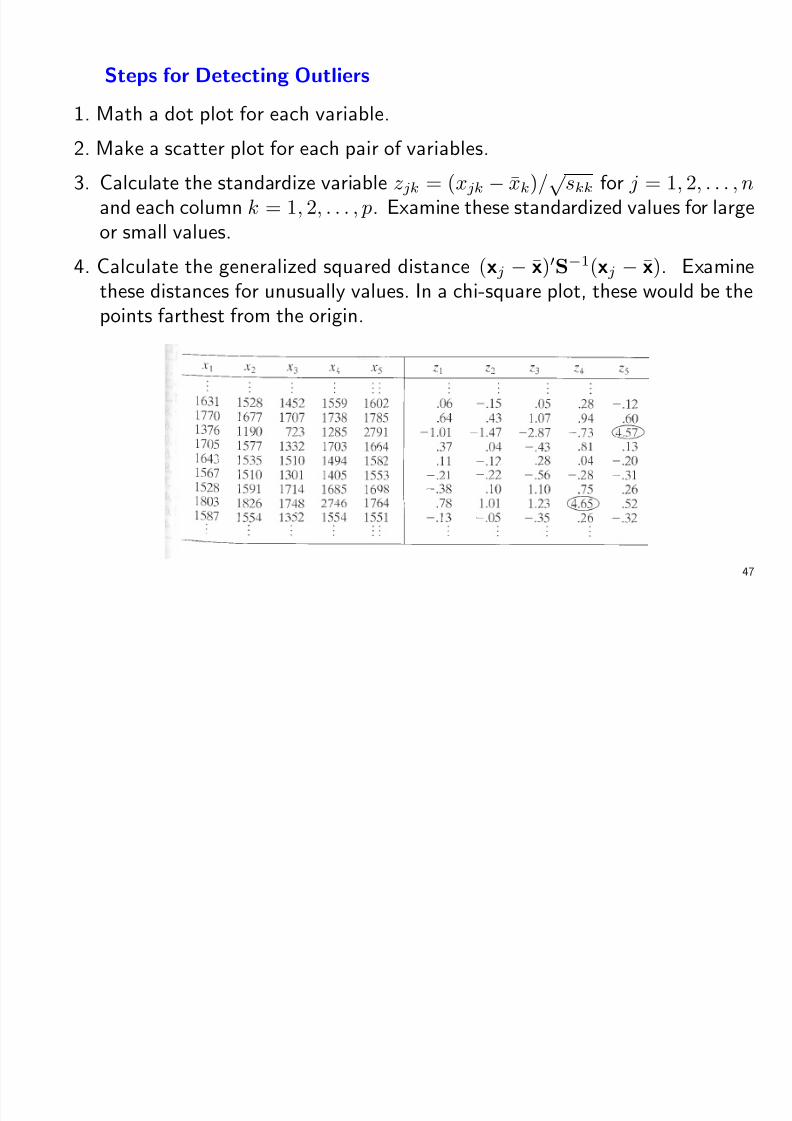
Steps for Detecting Outliers

1. Math a dot plot for each variable.

2. Make a scatter plot for each pair of variables.

3. Calculate the standardize variable zjk = (xjk − xk)/√

skk for j = 1, 2, . . . , nand each column k = 1, 2, . . . , p. Examine these standardized values for largeor small values.

4. Calculate the generalized squared distance (xj −

x)S−1(xj −

x). Examine

these distances for unusually values. In a chi-square plot, these would be thepoints farthest from the origin.

47



Example 3.15 (Detecting outliers in the data on lumber) Table 4.4 containsthe data in Table 4.3, along with the standardized observations. These dataconsist of four different measurements of stiffness x1, x2, x3 and x4, on each

n = 30 boards. Detect outliers in these data.

48



49



3.8 Transformations to Near Normality

If normality is not a viable assumption, what is the next step ?

• Ignore the findings of a normality check and proceed as if the data werenormality distributed. ( Not recommend )

• Make nonnormal data more “normal looking” by consideringtransformations of data. Normal-theory analyses can then be carriedout with the suitably transformed data.

Appropriate transformations are suggested by

1. theoretical consideration

2. the data themselves.

50





Example 3.16 (Determining a power transformation for univariate data)We gave readings of microwave radiation emitted through the closed doors of n = 42 ovens in Example 3.10. The Q-Q plot of these data in Figure 4.6

indicates that the observations deviate from what would be expected if theywere normally distributed. Since all the positive observations are positive, letus perform a power transformation of the data which, we hope, will produceresults that are more nearly normal. We must find that value of λ maximize thefunction (λ).

52



53



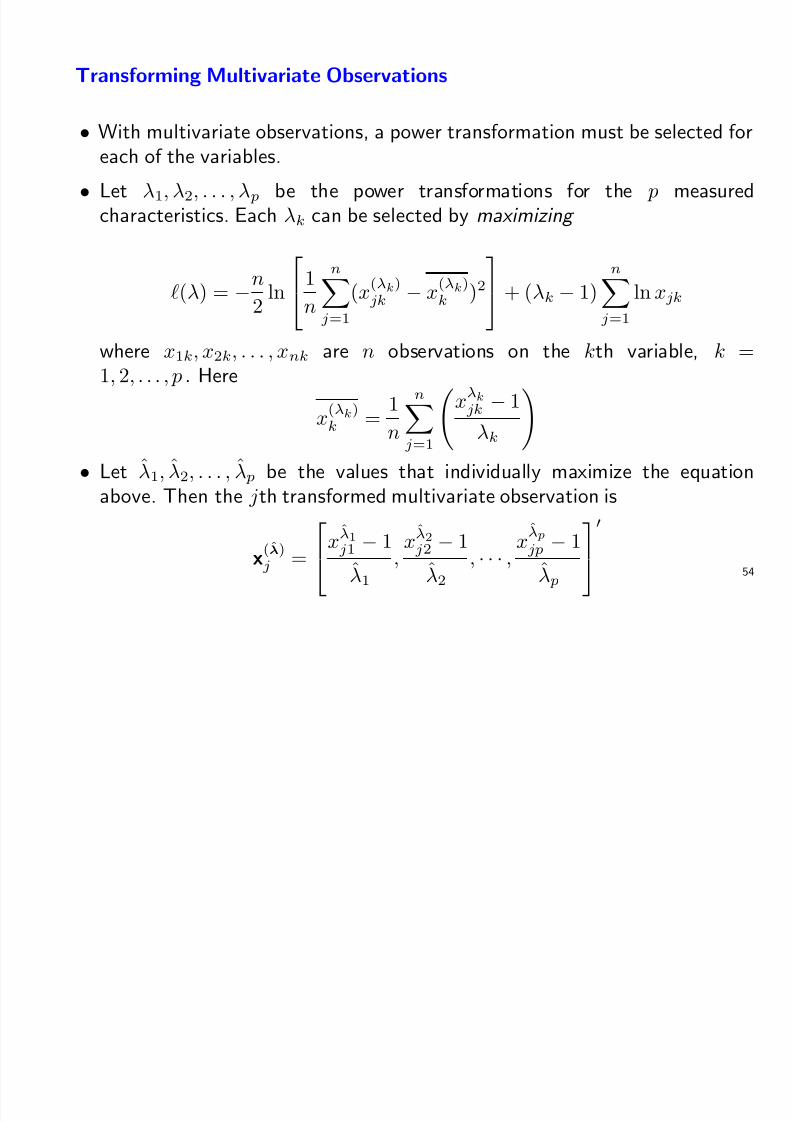
Transforming Multivariate Observations

• With multivariate observations, a power transformation must be selected foreach of the variables.

• Let λ1, λ2, . . . , λ p be the power transformations for the p measuredcharacteristics. Each λk can be selected by maximizing

(λ) = −n2

ln1

n

nj=1

(x(λk)jk − x(λk)

k )2 + (λk − 1)

nj=1

ln xjk

where x1k, x2k, . . . , xnk are n observations on the kth variable, k =1, 2, . . . , p . Here

x(λk)

k =

1

n

nj=1

xλkjk

−1

λk

• Let λ1, λ2, . . . , λ p be the values that individually maximize the equationabove. Then the jth transformed multivariate observation is

x(λ)

j =xλ1

j1

−1

λ1,

xλ2j2

−1

λ2, · · · ,

xλ pjp

−1

λ p

54



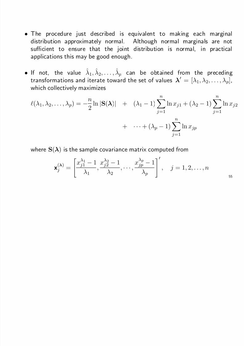
• The procedure just described is equivalent to making each marginaldistribution approximately normal. Although normal marginals are notsufficient to ensure that the joint distribution is normal, in practicalapplications this may be good enough.

• If not, the value λ1, λ2, . . . , λ p can be obtained from the precedingtransformations and iterate toward the set of values λ = [λ1, λ2, . . . , λ p],

which collectively maximizes

(λ1, λ2, . . . , λ p) = −n

2 ln |S(λ)| + (λ1 − 1)

nj=1

ln xj1 + (λ2 − 1)n

j=1

ln xj2

+ · · ·

+ (λ p−

1)n

j=1

ln xjp

where S(λ) is the sample covariance matrix computed from

x(λ)j = xλ1

j1 − 1

λ1

,xλ2j2 − 1

λ2

,

· · ·,

xλ pjp − 1

λ p

, j = 1, 2, . . . , n

55



Example 3.17 (Determining power transformations for bivariate data)Radiation measurements were also recorded though the open doors of then = 42 micowave ovens introduced in Example 3.10. The amount of radiation

emitted through the open doors of these ovens is list Table 4.5. Denote thedoor-close data x11, x21, . . . , x42,1 and the door-open data x12, x22, . . . , x42,2.Consider the joint distribution of x1 and x2, Choosing a power transformationfor (x1, x2) to make the joint distribution of (x1, x2) approximately bivariatenormal.

56



57





If the data includes some large negative values and have a single long tail, amore general transformation should be applied.

x(λ) =

{(x + 1)λ − 1}/λ x ≥ 0, λ = 0ln(x + 1) x ≥ 0, λ = 0−{(−x + 1)2−λ − 1}/(2 − λ) x < 0, λ = 2− ln(−x + 1) x < 0, λ = 2

Documents

Multi Varia Da 1