Embed Size (px)
Citation preview

ONDAS em MEIOS DESORDENADOS
Andre Nachbin, IMPA
Ondas em Meios Desordenados
Modelos Estocasticos e Aplicacoes,CBPF, 2007 Andre Nachbin IMPA http://www.impa.br/∼nachbin
ONDAS em MEIOS DESORDENADOS
Colaboradoresex-alunos de doutoradoJuan Carlos Munoz (Universidad del Valle, Cali, Colombia)
Daniel Alfaro (University of California at Irvine, EUA ⇒ visita IMPA, 2006)
William Artiles (Inst. de Fısica Teorica, Sao Paulo)
Ailın Fabregas (visita IMPA, 2007)
George Papanicolaou (Stanford Univ., EUA)
Jean-Pierre Fouque (University of Santa Barbara, EUA)
Josselin Garnier (Jussieu, Paris VII, Franca)
Knut Sølna (University of California at Irvine, EUA)
Wooyoung Choi (NJIT/New Jersey Institute of Technolgy, EUA)
Roberto Kraenkel (Inst. de Fısica Teorica, Sao Paulo)
Modelos Estocasticos e Aplicacoes,CBPF, 2007 Andre Nachbin IMPA http://www.impa.br/∼nachbin

ONDAS em MEIOS DESORDENADOS
Pesquisa em 3 frentes:
Parte A: Modelagem (FIS+MATE) e AnaliseAssintotica de EDPs/OPERADORES
Parte B: Analise Assintotica de SOLUCOES de modelosREDUZIDOS
Parte C: Analise Numerica e Computacao Cientıfica
Modelos Estocasticos e Aplicacoes,CBPF, 2007 Andre Nachbin IMPA http://www.impa.br/∼nachbin

ONDAS em MEIOS DESORDENADOS
PRIMEIRA aplicacao GEOFISICA com ONDAS emmeios DESORDENADOS
DIFUSAO APARENTE
Modelos Estocasticos e Aplicacoes,CBPF, 2007 Andre Nachbin IMPA http://www.impa.br/∼nachbin

ONDAS em MEIOS DESORDENADOS
MODELO ACUSTICO 1D:
PRESSURE WAVE
1D PROBLEM
VELOCITY PROFILE
EARTH CRUST
1
κ(z/ε2)
∂p
∂t+
∂u
∂z= 0, ρ(z/ε2)
∂u
∂t+
∂p
∂z= 0,
VELO. ALEATORIA c(z/ε2) ≡p
κ/ρ Dados: p(0, t) = u(0, t) = f (t/ε)
1/κ ≡ COMPRESSIBILIDADE da CROSTA terrestre ρ ≡ DENSIDADE
Modelos Estocasticos e Aplicacoes,CBPF, 2007 Andre Nachbin IMPA http://www.impa.br/∼nachbin

ONDAS em MEIOS DESORDENADOS
Situacao com UMA discontinuidade:
−1 −0.8 −0.6 −0.4 −0.2 0 0.2 0.4 0.6 0.8 1
−2
−1
0
1
2
3
INTERFACE
1 2
1/κ(z)∂p
∂t+
∂u
∂z= 0
ρ(z)∂u
∂t+
∂p
∂z= 0
Modelos Estocasticos e Aplicacoes,CBPF, 2007 Andre Nachbin IMPA http://www.impa.br/∼nachbin

ONDAS em MEIOS DESORDENADOS
Impedancia: ζi ≡ √ρiκi ; e tempo de transito x =
R z
0c−1(s)ds
−1 −0.8 −0.6 −0.4 −0.2 0 0.2 0.4 0.6 0.8 1
−2
−1
0
1
2
3
INTERFACE
1 2
Continuidade de p e u, e usando Invariantes de Riemann(const. ao longo de caracterıticas)...
TRANS. ≡ τ =2√
ζ1ζ2
ζ1 + ζ2REFL. ≡ σ =
ζ2 − ζ1
ζ1 + ζ2
CONSERV: τ2 + σ2 = 1
Modelos Estocasticos e Aplicacoes,CBPF, 2007 Andre Nachbin IMPA http://www.impa.br/∼nachbin

ONDAS em MEIOS DESORDENADOS
1D: VARIAS CAMADAS
ζ1
ζ1
ζ2 ζ
3
INFO
Modelos Estocasticos e Aplicacoes,CBPF, 2007 Andre Nachbin IMPA http://www.impa.br/∼nachbin

ONDAS em MEIOS DESORDENADOS
Ondas ACUSTICAS ∼ Ondas AQUATICAS (”Shallow Water Theory” )
Temos EDPs + PROBABILIDADE ⇒ N. & Sølna, Phys. Fluids 2003
−50 −40 −30 −20 −10 0 10−0.05
0
0.05
0.1
0.15
0.2
0.25
0.3
DISTANCIA RELATIVA A CHEGADA
MEIO MEDIANIZADO
ONDA TRANSMITIDA CROSTA ABAIXO ======>
PERFIL INICIAL
PERFIL SIMULADO
APROXIMACAO TEORICA
0 20 40 60 80 100 120 140 160 180 2000.6
0.8
1
1.2
1.4
CAMADAS NA CROSTA TERRESTRE PROFUNDIDADE =======>
MEIO DESORDENADO
Modelos Estocasticos e Aplicacoes,CBPF, 2007 Andre Nachbin IMPA http://www.impa.br/∼nachbin

ONDAS em MEIOS DESORDENADOS
Resultado DETERMINISTICO a partir de modelagem ESTOCASTICA:
0 5 10 15 20 25 30 35−0.02
0
0.02
0.04
0.06
0.08
0.1
distance from leading front [m]
trans
mitt
ed d
owng
oing
pul
se Impulse responses based on data and analysis
0 2 4 6 8 10 12 14−0.02
0
0.02
0.04
0.06
0.08
0.1
distance from front [m]
trans
mitt
ed d
owng
oing
pul
se
Impulse responses based on data and analysis
Modelos Estocasticos e Aplicacoes,CBPF, 2007 Andre Nachbin IMPA http://www.impa.br/∼nachbin
ONDAS em MEIOS DESORDENADOS
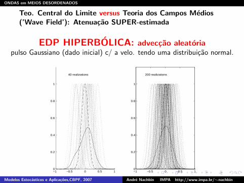
Teo. Central do Limite versus Teoria dos Campos Medios(’Wave Field’): Atenuacao SUPER-estimada
EDP HIPERBOLICA: adveccao aleatoriapulso Gaussiano (dado inicial) c/ a velo. tendo uma distribuicao normal.
−1 −0.5 0 0.5 10
0.2
0.4
0.6
0.8
1
200 realizations
−1 −0.5 0 0.5 10
0.2
0.4
0.6
0.8
1
40 realizations
Modelos Estocasticos e Aplicacoes,CBPF, 2007 Andre Nachbin IMPA http://www.impa.br/∼nachbin

ONDAS em MEIOS DESORDENADOS
EDOs ALEATORIAS com 1 ESCALA de TEMPO.
Teorema de Khasminskii(*): Sejam os PVIs ω ∈ (Ω, A, P)
dxε
dt= εF (t, xε; ω), xε(0) = x0
edy
dτ= F (y), y(0) = x0,
onde F (t, ·; ω) e um processo estocastico estacionario satisfazendo hipoteses de ergodicidade etc..., com
F (x) ≡ limT→∞
1
T
Z
T
0EF (t, x ; ω)dt.
Entao
sup0≤t
E|xε(t) − y(t)| ∼√
ε na escala de tempo 1/ε.
(*) R.Z. Khasminskii, On stochastic processes defined by differential equations with a small parameter,Theory Prob. Applications, Volume XI (1966), pp.211-228.
R.Z. Khasminskii, A limit-theorem for the solutions of differential equations with random right-hand sides,Theory Prob. Applications, Volume XI (1966), pp.390-406.
Modelos Estocasticos e Aplicacoes,CBPF, 2007 Andre Nachbin IMPA http://www.impa.br/∼nachbin
ONDAS em MEIOS DESORDENADOS
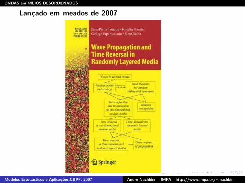
Lancado em meados de 2007
Modelos Estocasticos e Aplicacoes,CBPF, 2007 Andre Nachbin IMPA http://www.impa.br/∼nachbin

ONDAS em MEIOS DESORDENADOS
OUTRA aplicacao GEOFISICA com ONDAS emmeios DESORDENADOS
REFOCALIZACAO via REVERSAO TEMPORAL
Modelos Estocasticos e Aplicacoes,CBPF, 2007 Andre Nachbin IMPA http://www.impa.br/∼nachbin

ONDAS em MEIOS DESORDENADOS
I n a room inside the Waves and Acoustics Laboratory inParis is an array of microphones and loudspeakers. Ifyou stand in front of this array and speak into it, any-
thing you say comes back at you, but played in reverse. Your“hello” echoes—almost instantaneously—as “olleh.” At firstthis may seem as ordinary as playing a tape backward, butthere is a twist: the sound is projected back exactly towardits source. Instead of spreading throughout the room from
the loudspeakers, the sound of the “olleh” converges ontoyour mouth, almost as if time itself had been reversed. In-deed, the process is known as time-reversed acoustics, andthe array in front of you is acting as a “time-reversal mirror.”
Such mirrors are more than just a novelty item. They havea range of applications, including destruction of tumors andkidney stones, detection of defects in metals, and long-distance communication and mine detection in the ocean.
TIME-REVERSEDACOUSTICS
Arrays of transducers can re-create a sound and send it back to its source
as if time had been reversed. The process can be used to destroy kidney
stones, detect defects in materials and communicate with submarines
by Mathias Fink
DU
SA
N P
ET
RIC
IC
Modelos Estocasticos e Aplicacoes,CBPF, 2007 Andre Nachbin IMPA http://www.impa.br/∼nachbin

ONDAS em MEIOS DESORDENADOS
HELLO
Transdutores
Modelos Estocasticos e Aplicacoes,CBPF, 2007 Andre Nachbin IMPA http://www.impa.br/∼nachbin

ONDAS em MEIOS DESORDENADOS
They can also be used for elegant experiments in pure physics.The magic of time-reversed acoustics is possible because
sound is composed of waves. When you speak you producevibrations in the air that travel like ripples on a pondspreading out from the point where a stone splashed in. Afundamental property of waves is that when two of thempass through the same location, they reinforce each other iftheir peaks and troughs correspond, and they tend to canceleach other out if the peaks of one combine with the troughsof the other. This process takes place constantly wherever
back on exactly the reversed trajectory, which again wouldtotally alter the final outcome.
In contrast, wave propagation is linear. That is, a smallchange in the initial wave results in only a small change inthe final wave. Likewise, reproducing the “final” wave,moving in reverse but with the inevitable small inaccuracies,will result in the wave propagating and re-creating the “ini-tial” wave, also moving in reverse and having only relative-ly minor imperfections.
ACOUSTIC TIME-REVERSAL MIRROR operates in twosteps. In the first step (left) a source emits sound waves (orange)that propagate out, perhaps being distorted by inhomogeneitiesin the medium. Each transducer in the mirror array detects thesound arriving at its location and feeds the signal to a computer.
In the second step (right), each transducer plays back its soundsignal in reverse in synchrony with the other transducers. Theoriginal wave is re-created, but traveling backward, retracing itspassage back through the medium, untangling its distortionsand refocusing on the original source point.
RECORDING STEP TIME-REVERSAL AND REEMISSION STEP
ACOUSTIC SOURCE
HETEROGENEOUS MEDIUM
PIEZOELECTRIC TRANSDUCERS
ELECTRONIC
RECORDINGS
PLAYBACK
OF SIGNALS
IN REVERSE
SA
RA
H L
.D
ON
EL
SO
N
Modelos Estocasticos e Aplicacoes,CBPF, 2007 Andre Nachbin IMPA http://www.impa.br/∼nachbin

ONDAS em MEIOS DESORDENADOS
medical imaging, where one wishes to send the ultrasoundthrough fat, bone and muscle to targets such as tumors or
the problem is more complicated, but a single target can beselected by repeating the procedure. Consider the simplest
KIDNEY STONES can be targeted and broken up with ultra-sound by using the self-focusing property of a time-reversal mir-ror. An ultrasonic pulse emitted by one part of the array (a) pro-duces a distorted echo from the stone (b). A powerful time-reverse
of this echo passes through intervening tissues and organs, fo-cuses back on the stone (c) and breaks it up. Iterating the proce-dure improves the focus and allows real-time tracking as thestone moves because of the patient’s breathing.
ULTRASONIC PULSE ECHO FROM STONE TIME-REVERSED WAVE
CONTROL SYSTEM
RUBBER MEMBRANE
TRANSDUCER ARRAY
TIME-REVERSAL MIRROR
CYLINDRICAL TUB OF WATER
KIDNEY STONE
TRANSDUCER
ARRAY
PULSE OF
ULTRASOUND
SOUND REFLECTED
FROM KIDNEY
STONE
HIGH-POWER
TIME-REVERSED
PULSE
AL
FR
ED
T.K
AM
AJI
AN
a b c
Modelos Estocasticos e Aplicacoes,CBPF, 2007 Andre Nachbin IMPA http://www.impa.br/∼nachbin

ONDAS em MEIOS DESORDENADOS
cently researchers from the Scripps Institution of Oceanog-raphy in La Jolla, Calif., and the SACLANT Undersea Re-search Center in La Spezia, Italy, built and tested a 20-ele-ment TRM in the Mediterranean Sea off the coast of Italy[see illustration above]. Led by Tuncay Akal, WilliamHodgkiss and William A. Kuperman, they showed in waterabout 120 meters deep that their mirror could focus soundwaves up to 30 kilometers away. In a result similar to thesixfold enhancement in the scattering rod experiment, thetime-reversed beam was focused onto a much smaller spotthan the one observed with standard beam-forming sonar.
tects the echoes from one or more targets. The possible sce-narios are diverse, ranging from medical imaging to nonde-
FORMICHE DI GROSSETO
NATO RESEARCH VESSEL ALLIANCE
TRANSMITTER/RECEIVER ARRAY
(TIME-REVERSAL MIRROR)
PULSE
TRANSMITTER
RECEIVER ARRAY
120
MET
ERS
15 KILOMETERS
TRANSMITTED
SIGNAL
RECEIVED SIGNAL
TIME-REVERSAL MIRRORRECEIVER ARRAY
TIME-REVERSED SIGNAL
UNDERWATER COMMUNICATIONS can be en-hanced by using time-reversed acoustics to focus asignal. This technique was demonstrated in water120 meters deep near the island of Elba off the coastof Italy. A sound pulse was sent from the target loca-tion and recorded up to 30 kilometers away by anarray of transponders, distorted by refraction andmultiple reflections (red) from the surface and theseabed. The time-reversed signal sent by the arraywas well focused at the target location.
RESULTS from an underwater experimental run. Color con-tours indicate intensity of sound. The transmitted signal pulse(red circle) is greatly distorted at the time-reversal mirror, butwhen the time-reversed signal is played back (at left) it repro-duces a focused pulse at the receiver array (at right).
ALF
RED
T.K
AM
AJI
AN
;DAT
A F
RO
M T
UN
CAY
AK
AL
SACL
ANT
Unde
rsea
Re
sear
ch C
ente
r AN
D H
EEC
HU
N S
ON
G S
crip
ps In
stitu
tion
of O
cean
ogra
phy
FORMICHE
DI GROSSETO
ITALY
GIGLIO
ELBA
Mediterranean Sea
ALF
RED
T.K
AM
AJI
AN
;LA
UR
IE G
RA
CE
(inse
t)
Modelos Estocasticos e Aplicacoes,CBPF, 2007 Andre Nachbin IMPA http://www.impa.br/∼nachbin

ONDAS em MEIOS DESORDENADOS
ESQUEMATICAMENTE...
Modelos Estocasticos e Aplicacoes,CBPF, 2007 Andre Nachbin IMPA http://www.impa.br/∼nachbin

ONDAS em MEIOS DESORDENADOS
SUPER-RESOLUCAO!! “Multi-pathing”
Time-reversal aperture enhancement, JP Fouque, K Solna - SIAMMultiscale Modeling and Simulation, 2003.Super-resolution in time-reversal acoustics, P Blomgren, G Papanicolaou,H Zhao - The Journal of the Acoustical Society of America, 2002.
Modelos Estocasticos e Aplicacoes,CBPF, 2007 Andre Nachbin IMPA http://www.impa.br/∼nachbin

ONDAS em MEIOS DESORDENADOS
DESORDEM AJUDANDO!!Forcante ALEATORIO ⇒ choque viscoso: Fouque, Garnier & N., Physica D ’04.EDE ASSINTOTICAMENTE ⇒ elevacao da onda ≡ η(x , t) governada por
Burgers’ VISCOSA
14.8 15 15.2 15.4 15.6 15.8 16 16.2 16.4 16.6−0.01
−0.005
0
0.005
0.01 "Apparently viscous" profile at t = 6.25(1.25)15.0
α = 0.004; ε = 0.01
15 15.2 15.4 15.6 15.8 16 16.2 16.4 16.6 16.8 17−0.01
−0.005
0
0.005
0.01 "Inviscid Burgers" profile at t = 6.25(1.25)15.0
x ( All waves centered about solution at t= 6.25)
Initial profile centered at x = 10
Modelos Estocasticos e Aplicacoes,CBPF, 2007 Andre Nachbin IMPA http://www.impa.br/∼nachbin

ONDAS em MEIOS DESORDENADOS
MEIO ALEATORIO muito LONGO:
estamos no regime de LOCALIZACAO de Anderson
Modelos Estocasticos e Aplicacoes,CBPF, 2007 Andre Nachbin IMPA http://www.impa.br/∼nachbin

ONDAS em MEIOS DESORDENADOS
CENARIO para a TEORIA e SIMULACOES: Reversao Temporal
Perfis tıpicos: Gaussianas, dGaussiana/dx e onda Solitaria.
−2 −1.5 −1 −0.5 0 0.5 1 1.5
50
100
150
200
250
−10 0 10 20 30 40 50
50
100
150
200
250
−50 −40 −30 −20 −10 0 10 20 30 40 50−1
−0.8
−0.6
−0.4
−0.2
0
0.2
0.4
0.6
0.8
1x 10
−3
TRANSMITTED WAVE →← REFLECTED WAVE
TIME−REVERSED WAVE →
RANDOM MEDIUM HALF−SPACE
Modelos Estocasticos e Aplicacoes,CBPF, 2007 Andre Nachbin IMPA http://www.impa.br/∼nachbin

ONDAS em MEIOS DESORDENADOS
REFOCALIZACAO 1D TSUNAMI
−50 −40 −30 −20 −10 0 10 20 30 40 50
−5
0
5
x 10−4 t = 0
−50 −40 −30 −20 −10 0 10 20 30 40 50
−5
0
5
x 10−4 t = 5 0
Modelos Estocasticos e Aplicacoes,CBPF, 2007 Andre Nachbin IMPA http://www.impa.br/∼nachbin

ONDAS em MEIOS DESORDENADOS
LOCALIZACAO de ANDERSON: Alfaro et al., Comm. Math. Sci., ’07
z−AXIS
0 50 100 150 200 250 300 350 400
PULSE PROPAGATION
t = 0
t = 125
t = 250
t = 375
t = 500
z−AXIS0 50 100 150 200 250 300 350 400
TIME−REVERSED PULSE PROPAGATION
t = 0t = 125t = 250t = 375t = 500
Modelos Estocasticos e Aplicacoes,CBPF, 2007 Andre Nachbin IMPA http://www.impa.br/∼nachbin
ONDAS em MEIOS DESORDENADOS
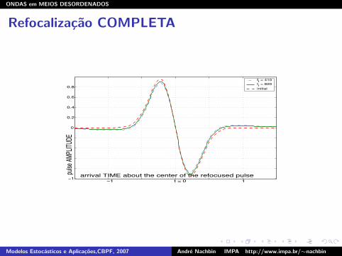
Refocalizacao COMPLETA
arrival TIME about the center of the refocused pulsepulse
AM
PLIT
UDE
−1 t = 0 1−1
0
0.2
0.4
0.6
0.8
tf = 410
tf = 820
initial
Modelos Estocasticos e Aplicacoes,CBPF, 2007 Andre Nachbin IMPA http://www.impa.br/∼nachbin

ONDAS em MEIOS DESORDENADOS
Regime Linear : Gaussiana
Clouet & Fouque, WMotion ’97, Fouque & N. , SIAM MMS ’04
Pulso refocalizado ≡ ηTR
(t) =1
2π
Z
e−iωt
η0(ω)
αmω2t′0
1 + αmω2t′0
!
dω.
αm =
Z
∞
0E m(0)m(x)dx M(s) = 1+m(s)
−40 −30 −20 −10 0 10 20 30 40 50
0
0.5
1
−40 −30 −20 −10 0 10 20 30 40 50−0.4−0.2
00.20.4
−40 −30 −20 −10 0 10 20 30 40 50−0.4−0.2
00.20.4
−40 −30 −20 −10 0 10 20 30 40 50−0.4−0.2
00.20.4
← REFLECTED SIGNAL TRANSMITTED SIGNAL →
TIME REVERSED SIGNAL →
(A)
(B)
(C)
(D)
t=0
t=t1
t=0
t=t1
∆ ∆ ∆ ∆ ∆ ∆ ∆ ∆ ∆ ∆ ∆ ∆ ∆ ∆ ∆ ∆ ∆ ∆ ∆ ∆ ∆ ∆ ∆ ∆
DISORDERED OROGRAPHY FLAT SECTION
h(ξ)
η
η
η
→
η
Modelos Estocasticos e Aplicacoes,CBPF, 2007 Andre Nachbin IMPA http://www.impa.br/∼nachbin

ONDAS em MEIOS DESORDENADOS
”Embaralhando e desembaralhando” um bit stream
TIME t
t=0 50 100 150 200 250 300 350 400 450
SIGNAL PROFILES
INITIAL SIGNAL
REFLECTED time−reversed SIGNAL
REFOCUSED SIGNAL
Modelos Estocasticos e Aplicacoes,CBPF, 2007 Andre Nachbin IMPA http://www.impa.br/∼nachbin

ONDAS em MEIOS DESORDENADOS
Parte A: ................ da palestra.
MODELOS REDUZIDOS; PORQUE?
SIMULACOES mais eficientes e ......melhor acesso a ANALISE/TEORIA MATEMATICA
Modelos Estocasticos e Aplicacoes,CBPF, 2007 Andre Nachbin IMPA http://www.impa.br/∼nachbin

ONDAS em MEIOS DESORDENADOS
Analise Assintotica de OPERADORES/EDPs:
MODELAGEM MATEMATICA
INTERIOR
Modelos Estocasticos e Aplicacoes,CBPF, 2007 Andre Nachbin IMPA http://www.impa.br/∼nachbin

ONDAS em MEIOS DESORDENADOS
Tıpica geometria de uma topografia DESORDENADA comMULTIPLAS-ESCALAS:
MULTISCALE TOPOGRAPHY
Modelos Estocasticos e Aplicacoes,CBPF, 2007 Andre Nachbin IMPA http://www.impa.br/∼nachbin

ONDAS em MEIOS DESORDENADOS
Eq. de EULER ou Teoria do Potencial Nao-Linear:
Equacoes em variaveis adimensionais:
βφxx + φyy = 0, em Ω ≡ CORPO FLUIDO,
com condicoes nao-lineares na ...SUPERFICIE LIVRE
φt + α2 (φ2
x + 1β φ2
y ) + η = 0
ηt + αφxηx − 1β φy = 0
em y = α η(x , t)
e uma cond. de Neumann na topografia DESORDENADA,
βγ h′( x
γ )φx + φy = 0 ao longo de y = −√
βh( xγ ),
onde a TOPOGRAFIA DESORDENADA e dada atraves de h.
α ≡ (amplitude/profundd), β ≡ (profundd/comprimento de onda)2, γ ≡ (desordem/comprmt de onda)
NAO-LINEARIDADE DISPERSAO DESORDEM
Modelos Estocasticos e Aplicacoes,CBPF, 2007 Andre Nachbin IMPA http://www.impa.br/∼nachbin

ONDAS em MEIOS DESORDENADOS
Tıpica geometria de uma topografia DESORDENADA comMULTIPLAS-ESCALAS:
MULTISCALE TOPOGRAPHY
Modelos Estocasticos e Aplicacoes,CBPF, 2007 Andre Nachbin IMPA http://www.impa.br/∼nachbin

ONDAS em MEIOS DESORDENADOS
Perfis Urbanos: problemas com Turbulencia Urbana
Modelos Estocasticos e Aplicacoes,CBPF, 2007 Andre Nachbin IMPA http://www.impa.br/∼nachbin

ONDAS em MEIOS DESORDENADOS
COORDENADAS CURVILINEAS: N. SIAP ’03
φξξ + φζζ = 0, −√
β < ζ < S(ξ, t).
Na fronteira livre η(x, t) ≈ N(ξ(x, 0), t)/M(ξ)
Nt +α
|J|φξNξ −1
|J|√
βφζ = 0.
φt +α
2|J|(φ2ξ + φ2
ζ) + η = 0.
Note que φζ = 0 em ζ = −√
β.
(∂ξξ + ∂ζζ) = |J|2∆xy ⇒ |J| ≡ (y 2ξ + y 2
ζ )|FS≈ y 2
ζ (ξ, 0) + O(ε2) (FRACA. N-LIN.)
Na fronteira livre o coeficiente metrico e M(ξ;√
β, γ) ≡ yζ(ξ, 0), onde
M(ξ;p
β, γ) =π
4√
β
Z ∞
−∞
h(x(ξo ,−√
β)/γ)
cosh2 π2√
β(ξo − ξ)
dξo .
Modelos Estocasticos e Aplicacoes,CBPF, 2007 Andre Nachbin IMPA http://www.impa.br/∼nachbin
ONDAS em MEIOS DESORDENADOS
ANALISE ASSINTOTICA de EDPs
Modelos Estocasticos e Aplicacoes,CBPF, 2007 Andre Nachbin IMPA http://www.impa.br/∼nachbin

ONDAS em MEIOS DESORDENADOS
Serie de potencias na viz. do fundo (transladado para) ζ = 0 Whitham 1974
φ(ξ, ζ, t) =
∞∑
n=0
ζn fn(ξ, t).
O potencial de velocidades (satisfiaz LAPLACE + NEUMANN)
φ(ξ, ζ, t) =
∞∑
n=0
(−β)n
(2n)!ζ2n ∂2nf (ξ, t)
∂ξ2n≈
N∑
n=0
[...]
Temos entao φ(x, y, t) ≡ cosh(k√
βy) exp(i(kx − ωt))
C 2(k) =ω2
k2=
1√βk
tanh(√
βk)
(VELO. de FASE)2 ≈ 1 − 1
3(√
βk)2 + 215
(√
βk)4 − 17315
(√
βk)6 + O((√
βk)8)
Relacao de dispersao truncada atraves da aprox. de Pade:C 2
a (k) = p(k)/q(k).
Modelos Estocasticos e Aplicacoes,CBPF, 2007 Andre Nachbin IMPA http://www.impa.br/∼nachbin

ONDAS em MEIOS DESORDENADOS
Madsen and Sørensen ’92, Nwogu ’93
Tomando a derivada de φ com respeito a ξ e avaliando a velo. emuma profundd. INTERMEDIARIA ζ = Z0 ∈ [0, 1]
φξ(ξ,Z0, t) ≡ u(ξ, t) = fξ −β
2Z0
2fξξξ + O(β2)
CONDICAO de FRONTEIRA LIVRE fica reduzida a famılia de equacoes BOUSSINESQ:
M(ξ)ηt +
[(
1 +α η
M(ξ)
)
u
]
ξ
+β
2
[(
Z02 − 1
3
)
uξξ
]
ξ
= 0
ut + ηξ + α
(
u2
2M2(ξ)
)
ξ
+β
2(Z0
2 − 1)uξξt = 0
Modelos Estocasticos e Aplicacoes,CBPF, 2007 Andre Nachbin IMPA http://www.impa.br/∼nachbin

ONDAS em MEIOS DESORDENADOS
famılia de equacoes BOUSSINESQ
M(ξ)ηt +
[(
1 +α η
M(ξ)
)
u
]
ξ
+β
2
[(
Z02 − 1
3
)
uξξ
]
ξ
= 0
ut + ηξ + α
(
u2
2M2(ξ)
)
ξ
+β
2(Z0
2 − 1)uξξt = 0
C 2 =ω2
k2=
1 − (β/2)(Z 20 − 1
3)k2
1 − (β/2)(Z 20 − 1)k2
ω2
k2=
1 + (β/15)k2
1 + 2(β/5)k2...e para o valor especial Z0 =
√
1/5
≈ 1 − 1
3(√
βk)2 +2
15(√
βk)4 − 475
(√
βk)6 + O((√
βk)8).
Modelos Estocasticos e Aplicacoes,CBPF, 2007 Andre Nachbin IMPA http://www.impa.br/∼nachbin

ONDAS em MEIOS DESORDENADOS
Seja Z0 =√
2/3 e uξ(ξ, t) = −M(ξ)ηt + O(α, β):
(M(ξ)η)t +
[(
1 +α η
M(ξ)
)
u
]
ξ
− β
6(M(ξ)η)ξξt = 0
ut + ηξ + α
(
u2
2M2(ξ)
)
ξ
− β
6uξξt = 0
Quintero and Munoz (Meth.Appl.Anal. ’04) demonstraram existencia, unicidade etc...
apos encontrarem uma integral de energia . Ferramentas semelhantes a Bona
& Chen ’98
(
I− β
6∂ξξ
)
−1[U] = Kβ ∗ U, Kβ(s) ≡ −1
2
√
6
βsign(s)e−
√6/β|s|
Modelos Estocasticos e Aplicacoes,CBPF, 2007 Andre Nachbin IMPA http://www.impa.br/∼nachbin
ONDAS em MEIOS DESORDENADOS
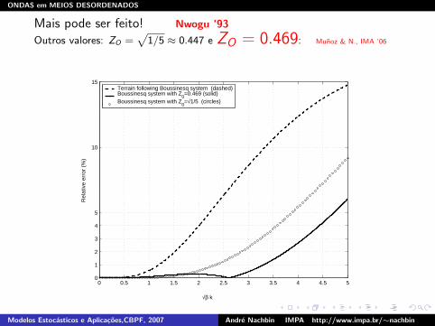
Mais pode ser feito! Nwogu ’93
Outros valores: ZO =p
1/5 ≈ 0.447 e ZO = 0.469: Munoz & N., IMA ’06
0 0.5 1 1.5 2 2.5 3 3.5 4 4.5 50
1
2
3
4
5
10
15R
elat
ive
erro
r (%
)Terrain following Boussinesq system (dashed)Boussinesq system with Z
0=0.469 (solid)
Boussinesq system with Z0=√1/5 (circles)
√β k
Modelos Estocasticos e Aplicacoes,CBPF, 2007 Andre Nachbin IMPA http://www.impa.br/∼nachbin

ONDAS em MEIOS DESORDENADOS
TOPOGRAFIA DESORDENADA
Comparamos modelos na JANELA ⇓
20 30 40 50 60 70 80 90 100 110 120−1
−0.8
−0.6
−0.4
−0.2
0
0.2
0.4
0.6
0.8
1
η at t = 50
β=0.05
ξ
T O P O G R A P H Y
Modelos Estocasticos e Aplicacoes,CBPF, 2007 Andre Nachbin IMPA http://www.impa.br/∼nachbin

ONDAS em MEIOS DESORDENADOS
TOPOGRAFIA DESORDENADA: espalhamento multiplo
ZO = 0.469
50 55 60 65 70 75 80−0.5
−0.4
−0.3
−0.2
−0.1
0
0.1
0.2
0.3
0.4
0.5
η at t=50 β=0.002
ξ
ZO =√
2/3 melhor valor para Analise Funcional
50 55 60 65 70 75 80
−0.4
−0.2
0
0.2
0.4
0.6
η at t = 50
ξ
β=0.002
Modelos Estocasticos e Aplicacoes,CBPF, 2007 Andre Nachbin IMPA http://www.impa.br/∼nachbin

ONDAS em MEIOS DESORDENADOS
NOVO ⇒ MODELO OTIMO
...atraves de analise assintotica em multiplas escalas.
Garnier, Kraenkel & N, PRE, October 2007
Modelos Estocasticos e Aplicacoes,CBPF, 2007 Andre Nachbin IMPA http://www.impa.br/∼nachbin

ONDAS em MEIOS DESORDENADOS
MODELO REDUZIDO (Boussinesq): M ≡ K ∗ h
Mηt +[
(1 +αη
M)u]
ξ− β
2(Z 2
0 − 1
3) [Mη]ξξt = 0 ,
ut + ηξ + α
[
u2
2M2
]
ξ
+β
2(Z 2
0 − 1)uξξt = 0 ,
MODELO COMPLETO:
βφxx + φyy = 0, em Ω ≡ CORPO FLUIDO periodico,
com condicoes nao-lineares na ...FRONTEIRA LIVRE
φt + α2 (φ2
x + 1β φ2
y ) + η = 0
ηt + αφxηx − 1β φy = 0
em y = α η(x , t)
e Neumann ao longo do fundo PERIODICO h(x)
βγ h′( x
γ )φx + φy = 0 ao longo de y = −√
βh( xγ ),
Modelos Estocasticos e Aplicacoes,CBPF, 2007 Andre Nachbin IMPA http://www.impa.br/∼nachbin

ONDAS em MEIOS DESORDENADOS
Buscando uma KdV EFETIVA
Buscamos atraves de uma expansao multi-escala na forma
η(t, ξ) = η0(t, ξ,ξ
ε) + εη1(t, ξ,
ξ
ε) + ...
u(t, ξ) = u0(t, ξ,ξ
ε) + εu1(t, ξ,
ξ
ε) + ...
onde ηj e uj sao periodicas em s = ξ/ε e as medias de η1 e u1
com respeito a s sao zero.
Modelos Estocasticos e Aplicacoes,CBPF, 2007 Andre Nachbin IMPA http://www.impa.br/∼nachbin

ONDAS em MEIOS DESORDENADOS
MODELO BOUSSINESQ: h(x) = 1 + n(x) = 1 + n1 sin(kx)
A KdV EFETIVA e
η0τ +3α∗
4(η2
0)X +β∗
6η0XXX = 0
onde X = x − v∗t e um sistema de referencia viajante. Emtermos dominantes
v∗2
= 1 − n21
2
√β0k
tanh(√
β0k)
α∗ = α0
(
1 +n2
1
2
"
„ √β0k
sinh(√
β0k)
«2
+1
2
√β0k
tanh(√
β0k)
#)
,
β∗ = β0
(
1 +n2
1
2
"
„
3
β0k2+ 1 − 3β0k
2
4(Z0
2 − 1
3)(Z0
2 − 1)
« „ √β0k
sinh(√
β0k)
«2
−5
2
√β0k
tanh(√
β0k)
–ff
.
sao os PARAMETROS da KdV EFETIVA .
Modelos Estocasticos e Aplicacoes,CBPF, 2007 Andre Nachbin IMPA http://www.impa.br/∼nachbin

ONDAS em MEIOS DESORDENADOS
TEORIA do POTENCIAL COMPLETA: Rosales & Papanicolaou ’83
A KdV EFETIVA e
η0τ +3α∗
4(η2
0)X +β∗
6η0XXX = 0
onde X = x − v∗t e
α⋆ =1
v⋆
„
α0 +α0
3
D
A2x
E
s− 2
3v⋆
˙
n′D
¸
b
«
pode ser expandido, no caso SENOIDAL, dando lugar a
α⋆ = α0
(
1 +n2
1
2
"
„
k√
β0
sinh(k√
β0)
«2
+1
2
k√
β0
tanh(k√
β0)
#
+ O(n31)
)
.
β⋆ = β0
1 +n2
1
2
»
3k√
β0
tanh3(k√
β0)− 11
2
k√
β0
tanh(k√
β0)
–
+ O(n31)
ff
.
Modelos Estocasticos e Aplicacoes,CBPF, 2007 Andre Nachbin IMPA http://www.impa.br/∼nachbin

ONDAS em MEIOS DESORDENADOS
Casando as duas KdVs
...atraves dos respectivos coeficientes de dispersao β⋆.Para β0k
2 pequenos, o casamento exato e obtido quando
Z0 =
√
2
3− 1√
5
Modelos Estocasticos e Aplicacoes,CBPF, 2007 Andre Nachbin IMPA http://www.impa.br/∼nachbin
ONDAS em MEIOS DESORDENADOS
Casando as duas KdVs
...atraves dos respectivos coeficientes de dispersao β⋆.Para β0k
2 pequenos, o casamento exato e obtido quando
Z0 =
√
2
3− 1√
5≃ 0.4685
Modelos Estocasticos e Aplicacoes,CBPF, 2007 Andre Nachbin IMPA http://www.impa.br/∼nachbin

ONDAS em MEIOS DESORDENADOS
Assim o modelo otimo da famılia Boussinesqpara a interacao onda-microestrutura e
Mηt +[
(1 +αη
M)u]
ξ+
β
2
(
√
1
5− 1
3
)
[Mη]ξξt = 0 ,
ut + ηξ + α
[
u2
2M2
]
ξ
− β
2
(
√
1
5+
1
3
)
uξξt = 0 .
Modelos Estocasticos e Aplicacoes,CBPF, 2007 Andre Nachbin IMPA http://www.impa.br/∼nachbin

ONDAS em MEIOS DESORDENADOS
Obrigado pela atencao.
IMPA, Rio de Janeiro.
Modelos Estocasticos e Aplicacoes,CBPF, 2007 Andre Nachbin IMPA http://www.impa.br/∼nachbin