Embed Size (px)
Citation preview

OTIMIZANDO MODELOS DE APRENDIZADO
DE RANQUEAMENTO COM BASE EM
AGREGACAO DE ARVORES DE DECISAO


CLEBSON CARDOSO ALVES DE SA
OTIMIZANDO MODELOS DE APRENDIZADO
DE RANQUEAMENTO COM BASE EM
AGREGACAO DE ARVORES DE DECISAO
Dissertacao apresentada ao Programa dePos-Graduacao em Ciencias da Com-putacao do Instituto de Ciencias Exatas daUniversidade Federal de Minas Gerais comorequisito parcial para a obtencao do grau deMestre em Ciencias da Computacao.
Orientador: Marcos Andre Goncalves
Belo Horizonte
Setembro de 2016

CLEBSON CARDOSO ALVES DE SA
OPTIMIZING ENSEMBLES OF BOOSTED
ADDITIVE BAGGED TREES FOR
LEARNING-TO-RANK
Dissertation presented to the GraduateProgram in Computer Science of the Uni-versidade Federal de Minas Gerais – Depar-tamento de Ciencia da Computacao. in par-tial fulfillment of the requirements for thedegree of Master in Computer Science.
Advisor: Marcos Andre Goncalves
Belo Horizonte
September 2016

c© 2016, Clebson Cardoso Alves de Sa.Todos os direitos reservados.
Sa, Clebson Cardoso Alves de
S111o Optimizing Ensembles of Boosted Additive BaggedTrees for Learning-to-Rank / Clebson Cardoso Alves deSa. — Belo Horizonte, 2016
xx, 69 f. : il. ; 29cm
Dissertacao (mestrado) — Universidade Federal deMinas Gerais – Departamento de Ciencia daComputacao.
Orientador: Marcos Andre Goncalves
1. Computacao. 2. Recuperaccao da informaccao.3. Floresta aleatoria. 4. Aprendizado de maquina.5. Aprendizado de ranqueamento.. I. Tıtulo.
CDU 519.6*73.(043)


“Computers aren’t supposed to be creative; they’re supposed to do what you tell them
to. If what you tell them to do is be creative, you get machine learning.”
(Pedro Domingos)
ix


Resumo
Recuperar informacao que realmente importe para o usuario e difıcil quando conside-
ramos grandes repositorios de dados como a web. Para aumentar a efetividade desta
tarefa de busca de informacao, sistemas tem tirado proveito da combinacao automatica
de funcoes de ranqueamento por meio de metodos de aprendizado de maquina, tarefa
tambem conhecida em recuperacao de informacao como aprendizado de ranqueamento.
Os metodos mais efetivos de aprendizado de maquina sao atualmente agregacoes de
arvores de decisao, tais como Florestas aleatorias e/ou tecnicas de impulsionamento
(e.g: RankBoost, Mart, LambdaMart). Nesta dissertacao, e proposta uma estrutura
que combina de maneira aditiva arvores de decisao, em especıfico Florestas Aleatorias
com Impulsionamento de maneira original para a tarefa de aprendizado de ranquea-
mento. Em particular, e explorado um conjunto de funcoes que tornam possıvel deduzir
quais amostras do conjunto de treino sao de difıceis predicao em um contexto de re-
gressao. Isso e realizado por meio da aplicacao de um conjunto seletivo de abordagens
de atualizacao da distribuicao de pesos das amostras para aumentar a performance
de ranqueamento do modelo de aprendizado de maquina. O modelo generico apresen-
tado nesta dissertacao aborda algumas instancias que consideram diferentes funcoes de
perda e diferentes maneiras de atualizar a importancia dos documentos. Nas analises
experimentais, os modelos foram capazes de superar todos os algoritmos considerados
do estado-da-arte em varias colecoes de dados. Outra vantagem da nossa estrutura de
aprendizado de maquina para ranqueamento e que ele e capaz de superar algoritmos
base avaliados considerando pequenas fracoes de treino e com taxas de convergencia
superior em todas as colecoes avaliadas. Isso mostra a vantagem em utilizar o nosso
modelo para problemas de ranqueamento, especialmente quando consideramos a difi-
culdade em se obter dados de treino.
Palavras-chave: Recuperacao de Informacao, Aprendizado de Ranqueamento, Apren-
dizado de Maquina, Florestas Aleatorias, Impulsionamento.
xi

Abstract
The task of retrieving information that really matters to the users is considered hard
when taking into consideration the current and increasingly amount of available infor-
mation. To improve the effectiveness of this information seeking task, systems have
relied on the combination of many predictors by means of machine learning methods,
a task also known as learning to rank (L2R). The most effective learning methods for
this task are based on ensembles of trees (e.g., Random Forests) and/or boosting tech-
niques (e.g., RankBoost, MART, LambdaMART). In this master degree dissertation,
we propose a general framework that smoothly combines ensembles of additive trees,
specifically Random Forests, with Boosting in an original way for the task of L2R. In
particular, we exploit a set of functions that enable us to smartly deduce the samples
that are considered hard to predict in a regression approach and apply a set of se-
lective weight updating strategy to effectively enhance the ranking performance. We
instantiate such a general framework by considering different loss functions, different
ways of weighting the weak learners as well as different types of weak learners. In our
experiments, our rankers were able to outperform all state-of-the-art baselines in all
considered datasets with statistical significance. Another important advantage of our
framework is that it is able of surpassing all baselines using just a small percentage of
the original training set, with the addition of faster convergence rates in all evaluated
collections. This shows the importance and potential of advantage of our approaches
over the baselines since training data with graded relevance judgments is very costly
and time-consuming to acquire.
Palavras-chave: Information Retrieval, Learning to Rank, Machine Learning, Ran-
dom Forest, Boosting.
xiii

List of Figures
2.1 Learning to Rank Model . . . . . . . . . . . . . . . . . . . . . . . . . . . . . . 9
4.1 Residues when minimizing the absolute loss-function . . . . . . . . . . . . 29
4.2 Residues when minimizing the median of a region. . . . . . . . . . . . . . . 29
4.3 Residues when minimizing the height of a regions. . . . . . . . . . . . . . . 32
4.4 Residues when minimizing the gradient descent with least square. . . . . . 33
6.1 Convergence analysis: NDCG as the number of boosting iterations increases. 45
6.2 Learning curve analysis for the boosting algorithms. . . . . . . . . . . . . . 47
6.3 BROOFgradient: Effect of out-of-bag samples versus entire training set. . . . 49
xv


List of Tables
4.1 Generalized BROOF-L2R: Possible instantiations. . . . . . . . . . . . . . . 27
5.1 Splitting strategy amongst the Folds . . . . . . . . . . . . . . . . . . . . . 36
5.2 Statistics of the evaluated collections in the main experiments. . . . . . . . 37
6.1 Mean Average Precision (MAP): Obtained results. . . . . . . . . . . . . . 42
6.2 Normalized Discounted Cumulative Gain (NDCG@10): Obtained results. . 43
6.3 NDCG@10 for the 4 instantiations of the proposed framework applied upon
the WEB10K in order to represent the full factor factorial design. . . . . . 51
6.4 Computation of effects with uniform initialization of weights . . . . . . . . 53
6.5 Computation of interactions – Using OOB . . . . . . . . . . . . . . . . . . 53
6.6 Allocation of variation explained by factors in all evaluated L2R sets. . . . 54
6.7 ANOVA using 95% of confidence level . . . . . . . . . . . . . . . . . . . . 56
xvii


Contents
Resumo xi
Abstract xiii
List of Figures xv
List of Tables xvii
1 Introduction 1
1.1 Motivation . . . . . . . . . . . . . . . . . . . . . . . . . . . . . . . . . . 2
1.2 Objectives . . . . . . . . . . . . . . . . . . . . . . . . . . . . . . . . . . 3
1.3 Achievements . . . . . . . . . . . . . . . . . . . . . . . . . . . . . . . . 4
1.4 Outline . . . . . . . . . . . . . . . . . . . . . . . . . . . . . . . . . . . . 5
2 Problem Statement and Algorithmic Background 7
2.1 Learning to Rank Framework . . . . . . . . . . . . . . . . . . . . . . . 7
2.2 Decision Trees . . . . . . . . . . . . . . . . . . . . . . . . . . . . . . . . 10
2.3 Ensemble Methods . . . . . . . . . . . . . . . . . . . . . . . . . . . . . 11
2.3.1 Random Forests . . . . . . . . . . . . . . . . . . . . . . . . . . . 11
2.3.2 Boosting . . . . . . . . . . . . . . . . . . . . . . . . . . . . . . . 12
3 Related Work 13
3.1 Major L2R Approaches . . . . . . . . . . . . . . . . . . . . . . . . . . . 13
3.2 Ensemble Design: Improving Efficiency . . . . . . . . . . . . . . . . . . 15
3.3 Deriving Ensembles of Decision Trees . . . . . . . . . . . . . . . . . . . 16
3.3.1 Random Forests . . . . . . . . . . . . . . . . . . . . . . . . . . . 16
3.3.2 Boosting . . . . . . . . . . . . . . . . . . . . . . . . . . . . . . . 17
3.3.3 Combining Bagged and Boosted Trees . . . . . . . . . . . . . . 19
4 Generalized BROOF-L2R 21
xix

4.1 Framework Description . . . . . . . . . . . . . . . . . . . . . . . . . . . 22
4.2 Possible Instantiations . . . . . . . . . . . . . . . . . . . . . . . . . . . 26
5 Experimental Protocol and Evaluation 35
5.1 Datasets . . . . . . . . . . . . . . . . . . . . . . . . . . . . . . . . . . . 35
5.2 Baselines . . . . . . . . . . . . . . . . . . . . . . . . . . . . . . . . . . . 36
5.3 Experimental Protocol and Setup . . . . . . . . . . . . . . . . . . . . . 38
6 Experimental Results 41
6.1 Benchmark Comparisons . . . . . . . . . . . . . . . . . . . . . . . . . . 41
6.1.1 Mean Average Precision – MAP . . . . . . . . . . . . . . . . . . 42
6.1.2 Normalized Discounted Cumulative Gain – NDCG . . . . . . . . 43
6.2 Behavioral Analysis . . . . . . . . . . . . . . . . . . . . . . . . . . . . . 44
6.2.1 Convergence Rate . . . . . . . . . . . . . . . . . . . . . . . . . . 44
6.2.2 Data Analysis . . . . . . . . . . . . . . . . . . . . . . . . . . . . 46
6.2.3 Validation Analysis . . . . . . . . . . . . . . . . . . . . . . . . . 48
6.3 Quantitative Analysis . . . . . . . . . . . . . . . . . . . . . . . . . . . . 50
6.3.1 Full Factorial Design . . . . . . . . . . . . . . . . . . . . . . . . 50
6.3.2 Computation of effects . . . . . . . . . . . . . . . . . . . . . . . 51
6.3.3 Allocation of variation . . . . . . . . . . . . . . . . . . . . . . . 53
6.3.4 Analysis of variance . . . . . . . . . . . . . . . . . . . . . . . . . 55
7 Conclusions and Future Work 59
7.1 The Framework . . . . . . . . . . . . . . . . . . . . . . . . . . . . . . . 59
7.2 Future Work . . . . . . . . . . . . . . . . . . . . . . . . . . . . . . . . . 60
7.2.1 A few Guidelines for Future Investigation . . . . . . . . . . . . . 61
Bibliography 63
xx

Chapter 1
Introduction
Today, we live in an era of massively available information, with a never-seen-before
(and increasing) rate of information production. It is not surprising that such a scenario
imposes hard to tackle challenges. For example, the availability of massive amounts of
data is not of great help if one is not able to effectively access the relevant content that
satisfies some user needs (informational, navigational or transactional) [Broder, 2002].
The problem arises when trying to make assertions of document relevance (im-
portance of web pages) to each individual user. This is quite difficult since the concept
of relevance is user dependent and therefore the same set of terms might have different
meanings when posed in comparison of two distinct users. This difficulty is mainly
attributed to the ambiguity of the query (e.g., “bond” may refer to the secret agent
James Bond, Original Electric String Quartet or a concept commonly used in finances)
[Santos et al., 2015] or simply due to the fact that the user may not express their
needs using the “best set of terms”. Another issue is that modifying the query length
by stretching or shrinking it to key terms does not assist the search engine in solving
the retrieval problem since it is known that every query, independent of its length, can
be considered ambiguous or ill-specified [Song et al., 2007].
Therefore, to answer this problem the main question that arises is: How to obtain
the “best rank” amongst all possible permutations of retrieved documents containing the
most relevant documents on top and non-relevant on the bottom?. The answer to this
specific question has become of extreme importance in the new era of mobile devices
with smaller screens, in which the need to focus only on the top most relevant results
is key [Pass et al., 2006, Granka et al., 2004]. This is even more important nowadays
when relevance depends on many other factors: location, timing, device capabilities
and many other conditions captured by wearables (smart watches).
Retrieval systems, such as search engines, question and answer (Q&A) forums,
1
2 Chapter 1. Introduction
and expert search systems serve exactly this purpose: given an information need, ex-
pressed in the form of a query (normally between 2 to 3 terms [Silverstein et al., 1999])
and a set of possible information units (e.g.: documents, web pages, images), the main
goal is to provide an ordered list of information units according to their relevance with
relation to the query [Manning et al., 2008]. The desideratum is to increase the likeli-
hood of satisfying a user’s information need in an effective manner by optimizing some
retrieval metric, which translates into pushing the truly relevant results on top of the
less relevant ones.
One of the key aspects that influence retrieval systems is how they determine the
relative relevance of candidate results in order to produce a ranked list containing the
most representative documents on top, and the least ones in the bottom. The quality
of those rankings is of primary importance in order to guarantee efficient and effective
access to relevant information (and, hopefully, the satisfaction of the user’s information
needs). Several approaches to generate such ranked lists do exist, being traditionally
performed by the specification of a function that is able to relate some user’s query
to the set of known (indexed) information units. Usually, ranking functions consider
several features, such as those that rely on the relatedness between query and possible
results by capturing the correlation of the list of documents and the searched subject
(e.g.: TF-IDF, BM25, edit distance, similarities in vector space models) or on link
analysis information that captures the “relative importance” of the document (e.g.,
PageRank, TrustRank) in some context (e.g., Web link structure) [Liu, 2011].
Unfortunately, to specify and fine-tune ranking functions turns out to be a ma-
jor problem, since it is known that most of them have sensitive parameters to the
subtle differences of the input space, what makes the learning process extremely ex-
pensive and time-consuming to obtain. Moreover, improving ranking effectiveness
is even more difficult, since it requires to effectively combine the individual features
[Gao and Yang, 2014], which increases the complexity of the problem as the number of
features grows with non-trivial interactions amongst them.
1.1 Motivation
This difficulty in effectively combining the best pieces of evidence in order to boost
ranking effectiveness motivates the use of Machine Learning (ML) algorithms to devise
such combinations. It is known that ML is capable of finding and combining several
pieces of evidence (predictors or features) in a non-trivial way (e.g., non-linearly) to-
wards optimizing some goal (a.k.a: loss functions) [Liu, 2011]. This is a field of study
1.2. Objectives 3
in information retrieval known as “Learning to Rank (L2R)”, whose primary goal is to
learn a model that is capable of automatically deriving the relevance score of unseen
documents.
More specifically, based on a set of {query |, documents} pairs with known rele-
vance judgments, the goal is to learn a function f(q, d) that is capable of accurately
devise the relevance prediction for a document d, with respect to a query q. Due to
ML importance in the information retrieval context, several approaches for L2R have
been proposed in the literature. As a matter of fact, ensemble methods based on
boosting such as RankBoost [Freund et al., 2003] or AdaRank [Xu and Li, 2007] and
bagged additive decision trees such as Random Forests [Breiman, 2001] or its variations
such as [Geurts and Louppe, 2011]), are deemed to be the techniques of choice for
L2R, achieving higher effectiveness in published benchmarks when compared to other
algorithms [Geurts and Louppe, 2011, Canuto et al., 2013].
Normally, ensemble strategies based on boosting are used as a wrapper iterati-
ve meta-algorithm that combines a series of weak learners (normally decision trees
or neural networks) [Drucker, 1997] in order to come up with an improved final
learner, focusing on hard-to-classify regions of the input space as the iterations in-
crease [Schapire and Freund, 2012]. Each weak learner is a predictor with generaliza-
tion capabilities better than random guessing and its concept is interchangeable with
the strong learnability concept since it is possible to transform a weak learner into a
improved strong learner [Schapire, 1990]. The ensemble strategies based on Random
Forest rely on the combination of several decision trees, learned with bagging (bootstrap
aggregation) of samples in the training set with additional randomization procedures
upon the feature vector (such as random feature selection) to produce decorrelated-
correlated trees — a requirement to guarantee its effectiveness [Breiman, 2001].
1.2 Objectives
In this work, we developed a general framework for L2R, named Generalized BROOF-
L2R that explores the advantages of boosting and Random Forests, by combining
them in a non-trivial fashion. More specifically, at each iteration of the boosting
algorithm, a Random Forest model is learned by training examples sampled according
to a probability distribution. Such probability distribution is updated at the end of
each iteration in order to force the subsequent learners to focus on hard to classify
regions of the input space. In particular, the use of RFs as weak learners has its
own advantages, since they are capable of providing robust estimates of expected error
4 Chapter 1. Introduction
through out-of-bag error estimates [Breiman, 1996b]. Moreover, by means of a selective
updating of the the weights of the out-of-bag samples, one can effectively slow down
the tendency of boosting strategies to overfit (a well-known phenomenon that becomes
critical as the noise level of the dataset being analyzed increases) [Salles et al., 2015].
As we shall detail in this master dissertation, the key aspects of the proposed
Generalized BROOF-L2R have to do with how to update the probability distribution
and how such update should be performed, as well as the underlying loss function
used to produce the final set of results. In this work, we discuss a set of possible
instantiations of the proposed general framework, in order to highlight the behavior
and potential of the proposed L2R solution.
In summary, the main research questions that we address are: (i) Can the com-
bination of these two machine learning approaches based on Boosting and Bagged
Trees help each other in order to enhance rank effectiveness in the context of L2R?
(ii) How should the samples distribution be updated at each iteration of the boosting
meta-algorithm? (iii) How should the loss functions be implemented in order to better
capture the main features of Boosting and Bagging in the context of L2R? (iv) Are
the instantiations computationally efficient? (v) Is it statistically and computationally
feasible to build and apply ensemble models in large real-world datasets?
The answers to those questions are scattered throughout the dissertation, and in
the next section, we highlight the main findings of this work.
1.3 Achievements
We develop a L2R framework named BROOF-L2R that allows the use of out-of-bag
samples as validation technique and at each boosting iteration we apply one of four
distinguished loss functions. Amongst all of our instances, the one that optimizes the
residue by minimizing the gradient descent loss function achieves the strongest results
in terms of Mean Average Precision (MAP) and Normalized Discounted Cumulative
Gain (NDCG), with significant improvements over the explored adversary algorithms
in 5 traditional benchmark datasets. Our alternative instances were also able to achieve
competitive (or superior) results when compared to the baselines in individual collec-
tions.
As our experimental evaluation shows, our general framework is able to produce
top-notch results with substantially less training samples and less iterations compared
to the evaluated baselines. Such data efficiency and high generalization capabilities
are key to guarantee practical feasibility since obtaining labeled data and machinery-
1.4. Outline 5
power are very costly. We also provide extensive statistical analysis of our findings
using well-known statistical designs and hypothesis tests to demonstrate the benefits
of the BROOF-L2R framework.
To summarize, the contributions of this work are three-fold: (i) we provide a
general framework for L2R that is able to combine two strong methods (boosting and
Random Forests) in an original way, which can be specialized in several ways and
produce highly effective L2R solutions; (ii) we propose and discuss a set of alternative
instantiations of such a framework, in order to highlight the behavior and effectiveness
of each possible choice; and (iii) we advance the state of the art in L2R by means of
some instantiations of our proposed framework that are able to outperform top-notch
solutions, according to an extensive benchmark evaluation considering five datasets
and seven L2R baseline algorithms.
The potential of our approach is demonstrated by two published papers, one
in a national level [de Sa et al., 2015] (KDMile) and another in an international level
[de Sa et al., 2016], in which this last one is the major Information Retrieval conferen-
ce (SIGIR). In the first paper, is shown an initial study of this two machine learning
algorithms applied in the L2R context with a general idea of how they could be merged
into a single elegant algorithm. The second published paper deepens into the possible
ways of making this two algorithms work together by defining an extensible and general
framework for L2R based in the combination of this two ensemble machines.
The following section contains a Roadmap with a brief description of the organi-
zation of each chapter of this dissertation.
1.4 Outline
The remainder of this work is described as follows:
• In Chapter 2, we formalize what is the task of L2R and the main differences
from other classification and regression problems. We also introduce the nota-
tions and conventions that are necessary to better understand the techniques and
algorithms used in the proposed framework.
• In Chapter 3, we provide a brief description of related work using Boosting,
committee of additive trees such as Bagging and RF or even the combination or
enhancement of one or another approach in the context of L2R.
• In Chapter 4, we discuss the BROOF-L2R framework and how to instantiate it

6 Chapter 1. Introduction
by modifying individual steps that generate stronger models with higher genera-
lization capabilities.
• In Chapter 5, we describe the experimental statistical methods used to summarize
the obtained results.
• In Chapter 6, we detail our results considering the experiments performed as
described in Chapter 5.
• Finally, in Chapter 7, we conclude the dissertation, summarizing our main find-
ings and proposing some directions for further investigation.

Chapter 2
Problem Statement and Algorithmic
Background
In this chapter, we briefly describe what is L2R and give an overview of the algorithms
used in the presented framework.
2.1 Learning to Rank Framework
As described by [Baeza-Yates and Ribeiro-Neto, 1999], the task of ranking is at the
core of information retrieval by directly retrieving to individual users an ordered list
of documents containing the most relevant documents at the top while pushing away
the less relevant ones. This is usually done by using a set of ranking functions that
are combined in order to increase ranking effectiveness. To achieve this effectiveness
in a feasible way, ML approaches are used to figure out the relevance of a document
regarding pairs of query and documents [He et al., 2008].
Although it is known that there exists research in L2R that considers semi-
supervised learning, such as inductive approaches that propagate the ground-truth
known labels to the unknown documents, or even completely unsupervised ones, such
as on-line L2R by using implicit feedback, in this work we only consider it as a super-
vised technique which exploits the query dimension. Therefore, we can use any ML
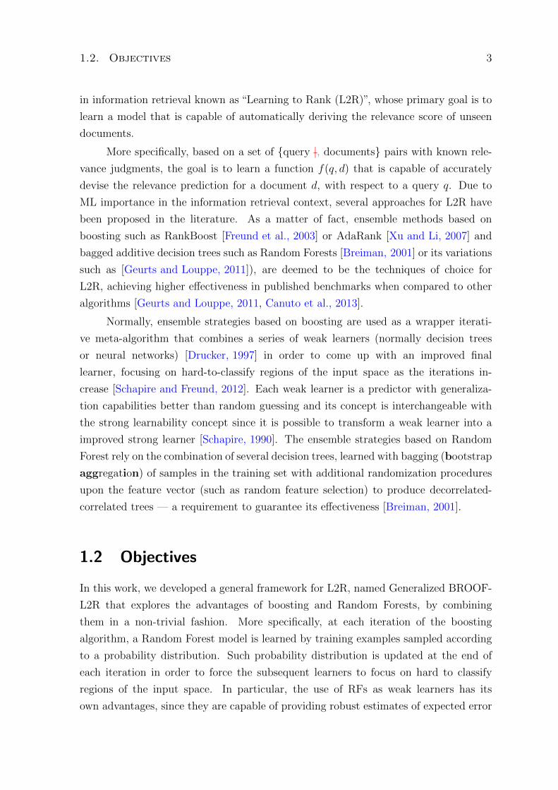
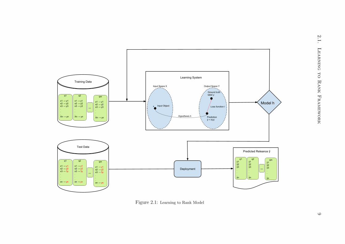
algorithm for classification or regression to estimate the relevance of a document. To
better exemplify, Figure 2.1 shows a chart that aids to visualize how ML is applied in
the L2R context. As any supervised classification approach, to build a ML model to
rank documents, it is necessary to have a training dataset that is composed of a set
of queries Q = {q1, q2, q3, . . . , qm}. Each individual query q is accompanied by a set of
7

8 Chapter 2. Problem Statement and Algorithmic Background
documents X = {x1, x2, x3, . . . , xn} that are represented as feature vectors, in which
each feature is a ranking function by itself or a combination of them.
As we can also see in Figure 2.1, each document in the training set has its own
annotated relevance judgment yn that identifies the “importance” of a document xn to
answer a given query qm. Such importance of a document xn may vary for different
queries. The representativeness of a document is usually defined as a binary or multi-
graded relevance judgment. The first one implies that a document can either be 0)
non-relevant or 1) relevant for a given search. The second one considers that the
importance of a document can range in a graded scale, for instance, from 0 to 4, being
0 the least relevant and 4 the most relevant one [Liu, 2011].
Given the training set, a machine learning system is applied to the discriminative
data to figure out a hypothesis h that will evaluate each sample document in the input
space X and then assign a prediction y for each document based on its features h(xn).
By means of this prediction, it is possible to compute its distance from the ground
truth relevance y, which allows us to identify by means of an evaluation metric the
generalization capabilities of an algorithm by using some loss function l.
After the construction of the model, it is possible to refine its predictions by eva-
luating different parameters using cross-validation techniques. When the final model
is ready, it is possible to apply the resulting mechanism in a test set by passing a
list of documents for individual queries and, as a result, to obtain the prediction for
each document in the form of a class, in case of classification, or regression scores
values. Although some papers mention that, for L2R the use of classification or re-
gression algorithms are statistically equivalent and that the best approach is dataset
dependent [Geurts and Louppe, 2011], in this work we consider only the regression ap-
proach, since it provides a way of differentiating how much the prediction of a document
is more important than another one. After the computation of the importance of the
documents, the last step is to sort the documents according to its predicted score y
[Liu, 2009, Liu, 2011].
2.1
.L
earnin
gto
Rank
Fram
ew
ork
9
Hypothesis h
Test Data
q1 x1 → y1 x2 → y2x3 → 3y...xn → yn
...
q2 x1 → y1 x2 → y2x3 → 3y...xn → yn
qm x1 → y1 x2 → y2x3 → 3y...xn → yn
Input Space X Output Space Y
x
Predictionŷ = h(x)
Loss function l
Ground truth label y
Input Object
Learning SystemTraining Data
q1 x1 → y1 x2 → y2x3 → y3...Xn → yn
...
q2 x1 → y1 x2 → y2x3 → y3...Xn → yn
qm
x1 → y1 x2 → y2x3 → y3...Xn → yn
Model h
q1ŷ1 ŷ2ŷ3...ŷn
...
q2ŷ1 ŷ2ŷ3...ŷn
qmŷ1 ŷ2ŷ3...ŷn
Predicted Releance ŷ
Deployment
Figure 2.1: Learning to Rank Model

10 Chapter 2. Problem Statement and Algorithmic Background
2.2 Decision Trees
Decision trees are known to be one of the most popular ML algorithms amongst re-
searchers. Its popularity is mainly due to: (i) their high generalization capabilities; (ii)
their generality, allowing their application in many fields of study such as statistics,
machine learning, data mining, pattern recognition and many others; (iii) their inter-
pretability, since it is possible to trace the pieces of evidence by descending through
the nodes of the tree and verifying the many criteria of impurity chosen in order to
split the data through the nodes [Maimon and Rokach, 2010].
There are many ways of instantiating a model based on decision trees: CART
[Breiman et al., 1984], ID3 [Quinlan, 1986], C4.5 [Quinlan, 1993] are some of the most
popular algorithms. In this work, we only highlight the use of CART as our primary
algorithm of study, since there are many freely available implementations of it such
as the highly known python library by [Pedregosa et al., 2011]. The CART acronym
stands for classification and regression trees, and it works by recursively dividing the
input space by making orthogonal splits considering an univariate splitting criteria of
impurity [Breiman et al., 1984].
For classification problems usually Gini Index, Entropy or Classification Error
are used as measure of impurity. These three measures are described in Equations 2.1,
2.2 and 2.3:
Classification Error = 1−max[p(i|t)] (2.1)
Gini = 1−c−1∑i=0
[p(i|t)]2 (2.2)
Entropy = −c−1∑i=0
p(i|t)log2p(i|t), (2.3)
in which c is the total amount of individual annotated relevance judgments of
documents in a given node, p is the probability of documents with class i regarding
the total number of documents t. For the regression case, the most known equivalent
splitting criteria is known as Mean Squared Error (MSE) shown in Equation 2.4:
MSE = minj,s
minc1
∑xi∈R1(j,s)
(yi − c1)2 + minc2
∑xi∈R2(j,s)
(yi − c2)2 , (2.4)
In here R1 and R2 are pairs of half-planes of a node t that are chosen by a

2.3. Ensemble Methods 11
greedy algorithm that considers a splitting variable j and a split point s. The inner
minimization considers the average of documents in each individual region given by
c1 and c2. The greedy algorithm is necessary in order to maintain the feasibility of
the solution (required in order to process large amounts of data) since to find the best
tree structure is considered NP-hard [Hancock et al., 1996]. This splitting criterion
is recursively processed until one of the stopping rules are achieved (total number of
nodes, the total number of leaves, the tree depth, the number of attributes used), or
until all tree nodes are pure, which achieves the tree’s maximum length. The problem
of letting the tree grow to its maximum extent is that, as it grows, it starts to loose
its generalization capabilities and probably overfitting on training or validation set,
which requires a set of pruning steps in order to reduce the complexity of the model.
To further understanding decision trees, we refer the reader to [Breiman et al., 1984,
Quinlan, 1986, Tan et al., 2005, Maimon and Rokach, 2010].
2.3 Ensemble Methods
Although there is no formal definition of what is an ensemble method, theoretical and
empirical studies have shown the importance of committee of aggregated classifiers.
The general classifier which assembles the individual ones using a combiner is usually
better than the single counterparts [Kuncheva, 2014]. The two most known ensembles
of additive trees are Random Forests and Boosting, and in the two following subsections
we provide a brief overview of each one of this two ML models.
2.3.1 Random Forests
As a variant of bagging (bootstrap aggregation) approach, RF is one of the most
powerful ML ensemble techniques, being extremely efficient and effective in sev-
eral tasks such as genome data analysis [Chen and Ishwaran, 2012], image detection
[Antonio Criminisi, 2009], tag recommendation [Canuto et al., 2013] and name disam-
biguation [Treeratpituk and Giles, 2009] to name a few. Its high generalization power
is mainly due to its efficiency in minimizing the variance while not increasing too much
the bias. Thus, when building the individual trees of the ensemble, a set of random-
ization techniques are applied upon the training data and feature vector of documents.
Since the randomization of training samples are performed with resampling, a Poisson
distribution estimates that roughly 63% of the original set of documents should be
used. The remaining 37% of the samples, named as out-of-bag (oob) samples, may be
used as validation technique of the fitted model. The randomization of the features

12 Chapter 2. Problem Statement and Algorithmic Background
is usually the proportion of√p in which p refers to the dimensionality of predictors
and the intuition of this randomization is to decrease even further the variance of the
model [Breiman, 2001].
2.3.2 Boosting
Boosting is a meta-algorithm that exploits the weak learner assumption, improving
the efficiency of any classifier in which the accuracy is better than random guessing
[Solomatine and Shrestha, 2004]. To increase the likelihood of getting a better classi-
fier in each round of the iterative procedure it modifies the importance of samples in
the input space by resampling the documents according to a given probability distri-
bution function [Quinlan, 1996] or by associating weights to each training sample and
iteratively modifying this weight distribution [Solomatine and Shrestha, 2004].
The associative weights’ distribution has the same uniform probability distribu-
tion at the initial step, and as the number of iterations grows the weights are modified in
order to represent the samples that are more difficult to predict. This updating scheme
of the distribution has the intention of iteratively identifying the “hard to predict” re-
gions of the input space and heuristically building new weak classifiers on specific hard
to predict regions. As new specialized classifiers are built upon these hard to predict
regions the bias tends to minimize. A problem with this technique is that boosting is
very susceptible to noise data, which can cause overfitting as the number of iterations
grow [Schapire, 1999].
As a final remark, in contrast to the RF approach, the variation required in
boosting to identify the hard to predict samples is by fitting decision stumps or small
trees, whilst RF tends to keep variation through bagging while fitting fully grown trees.

Chapter 3
Related Work
Due to the effectiveness of boosting and RF, there are plenty of research aiming at
improving and/or assembling one of these two ML mechanisms. Some of them can be
found in [Fernandez-Delgado et al., 2014] and [Tax et al., 2015]. The first one shows
a comparison of 179 algorithms and the second one is a selective cross-benchmark
with specifically tailored solutions to improve document retrieval containing 87 L2R
approaches. The most interesting aspect of these two works is that independent of
the search domain, the top performers are always ensembles of additive trees. In the
sections that follow, we provide a brief description of related work that attempts at
improving ensemble of additive trees approaches.
3.1 Major L2R Approaches
Learning to Rank solutions are divided into three major approaches: pointwise, pair-
wise and listwise. Pointwise L2R algorithms are probably the simplest (yet successful)
approaches, directly translating the ranking problem to a classification/regression one.
In this case, the training set for the supervised learning algorithm consists of pairs
{qm, (xmn , ymn )} of queries qm and a list of associated documents xmn (nth document of
query m), each one with its relevance judgment ymn (relevance judgment of document
xn of query qm). In this case, each triple (qm, xmn , y
mn ) is considered to be a single
training example. The goal is to learn a classifier/regressor model capable of accu-
rately predicting the relevance score of a document x, with relation to a query qm,
thus producing a partial ordering over documents. Pairwise algorithms, on the other
hand, transform the ranking problem into a pairwise classification problem. In this
case, learning algorithms are used to predict orders of document pairs, thus exploring
more ground-truth information than the pointwise approaches. Unlike both mentioned
13
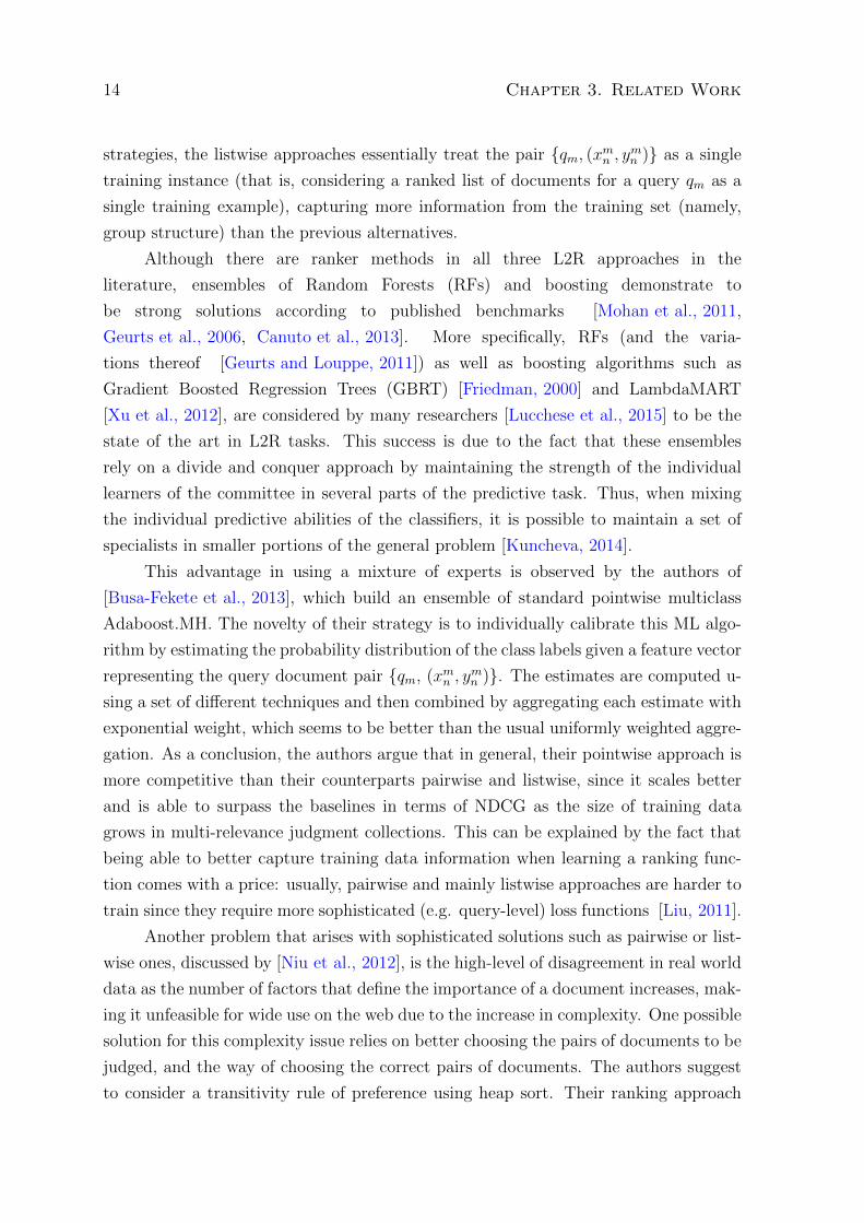
14 Chapter 3. Related Work
strategies, the listwise approaches essentially treat the pair {qm, (xmn , ymn )} as a single
training instance (that is, considering a ranked list of documents for a query qm as a
single training example), capturing more information from the training set (namely,
group structure) than the previous alternatives.
Although there are ranker methods in all three L2R approaches in the
literature, ensembles of Random Forests (RFs) and boosting demonstrate to
be strong solutions according to published benchmarks [Mohan et al., 2011,
Geurts et al., 2006, Canuto et al., 2013]. More specifically, RFs (and the varia-
tions thereof [Geurts and Louppe, 2011]) as well as boosting algorithms such as
Gradient Boosted Regression Trees (GBRT) [Friedman, 2000] and LambdaMART
[Xu et al., 2012], are considered by many researchers [Lucchese et al., 2015] to be the
state of the art in L2R tasks. This success is due to the fact that these ensembles
rely on a divide and conquer approach by maintaining the strength of the individual
learners of the committee in several parts of the predictive task. Thus, when mixing
the individual predictive abilities of the classifiers, it is possible to maintain a set of
specialists in smaller portions of the general problem [Kuncheva, 2014].
This advantage in using a mixture of experts is observed by the authors of
[Busa-Fekete et al., 2013], which build an ensemble of standard pointwise multiclass
Adaboost.MH. The novelty of their strategy is to individually calibrate this ML algo-
rithm by estimating the probability distribution of the class labels given a feature vector
representing the query document pair {qm, (xmn , ymn )}. The estimates are computed u-
sing a set of different techniques and then combined by aggregating each estimate with
exponential weight, which seems to be better than the usual uniformly weighted aggre-
gation. As a conclusion, the authors argue that in general, their pointwise approach is
more competitive than their counterparts pairwise and listwise, since it scales better
and is able to surpass the baselines in terms of NDCG as the size of training data
grows in multi-relevance judgment collections. This can be explained by the fact that
being able to better capture training data information when learning a ranking func-
tion comes with a price: usually, pairwise and mainly listwise approaches are harder to
train since they require more sophisticated (e.g. query-level) loss functions [Liu, 2011].
Another problem that arises with sophisticated solutions such as pairwise or list-
wise ones, discussed by [Niu et al., 2012], is the high-level of disagreement in real world
data as the number of factors that define the importance of a document increases, mak-
ing it unfeasible for wide use on the web due to the increase in complexity. One possible
solution for this complexity issue relies on better choosing the pairs of documents to be
judged, and the way of choosing the correct pairs of documents. The authors suggest
to consider a transitivity rule of preference using heap sort. Their ranking approach

3.2. Ensemble Design: Improving Efficiency 15
basically builds an ensemble using a listwise loss function to model the order of top k
elements and a pairwise loss function to model the preference of top items to each of
the k items. The final model is the ensemble of listwise approaches SVMMAP, AdaRank
and ListNet combined with the pairwise models RankSVM, RankBoost and RankNet.
This ensemble technique minimizes the complexity of the main pairwise problem by
only evaluating a few combination of documents, instead of judging all possible pairs
of documents during the creation of the model.
Although we devise a series of loss functions that work upon the queries dimen-
sion to improve the ranking performance towards minimizing the residues, we do not
use any information retrieval metric that directly computes the current relevance of
the documents being ranked at a given iteration to improve the ranking effectiveness.
Therefore, we see our approaches as pointwise methods. In the following section, we
highlight some related work that attempts at improving the tree structure of ensemble
models in order to improve its efficiency, which is a requirement to be competitive
nowadays.
3.2 Ensemble Design: Improving Efficiency
Although ensemble machines generate very effective models, they are not without draw-
backs. The general ensembles of additive trees are usually known to require large
amounts of memory due to the large number of trees in the final committee. This
becomes a real problem when considering general purposes hand-held systems such as
wearables, smartphones, embedded systems and Web applications.
To overcome this issue, the authors of the Boosted Random Forest
[Mishina et al., 2014] algorithm build an ensemble method by introducing boosting
into a RF. This introduction of boosting is intended to reduce the amount of memory
allocated for the RF by effectively applying the boosting algorithm to each individual
tree of the ensemble and then heuristically selecting only the trees that increase the
overall effectiveness of the ensemble in the training stage process. According to their
findings, this process reduces the number of trees on the ensemble while increasing the
effectiveness of the final model. Therefore, they are applying boosting to individual
trees and then assembling them into a RF model containing only the best learners.
As shown in their experimental results, this process is able to effectively reduce the
number of individual trees in the final ensemble with better ranking performance and
low memory cost.
Another enhancement on an ensemble of additive trees towards the performance

16 Chapter 3. Related Work
of the models is the QuickScorer algorithm, which modifies the tree structure in order
to boost up the tree efficiency of the final model. The novelty of the QuickScorer is the
use of bitwise operations to traverse the tree in a feature-wise order, thus making the
tree traversal cache-aware. According to the authors [Lucchese et al., 2015], the trees
in the ensemble are simultaneously traversed by interleaving the features of each tree,
which enables efficiency up to 6.5 times faster than the original tree. Another attempt
of improving the tree ensemble by the authors [Lucchese et al., 2016b] is through vec-
torization of the tree in the QuickScorer algorithm, which enables them to parallelize
the tree traversal in the algorithm using SIMD extensions.
Another enhancement in an ensemble of an additive tree is proposed in
[Lucchese et al., 2016a], which suggests a series of modifications in the structure of
the ensemble by making a set of pruning strategies in each tree of the ensemble and
then removing trees that are too much correlated in their structure. This cleaning up
of trees have the same purpose of the aforementioned work by [Mishina et al., 2014],
but instead of minimizing the complexity of the final ensemble using boosting, they
re-weight the trees that were left on the ensemble using a greedy line search algorithm
that optimizes the weights of the trees by minimizing a given loss function. According
to their findings, this strategy, named CLEaVER, is up to 2.6 times faster than the
original ensemble without losing its generalization effectiveness.
3.3 Deriving Ensembles of Decision Trees
This section highlights a series of works that attempt to derive improved versions of
an ensemble of decision trees in order to optimize its effectiveness. We first highlight
the improvements over RF derivations, then we describe a few works that make some
derivations over the traditional boosting meta-algorithm. For last, we cite a few works
that elegantly improve ensemble models by combining these two strategies into a single
committee.
3.3.1 Random Forests
As mentioned so far, it is natural to expect several extensions of RF and Boosting not
only towards optimizing its efficiency but improving its effectiveness as well. One such
extension in the classification realm for ranking is proposed by [Jiang, 2011], which
derives a RF model by modifying the tree node measure of impurity with the replace-
ment of the traditional Information Gain (when using entropy as measure of impurity)
for the Average Gain. According to the authors, this minimizes the tendency of Infor-
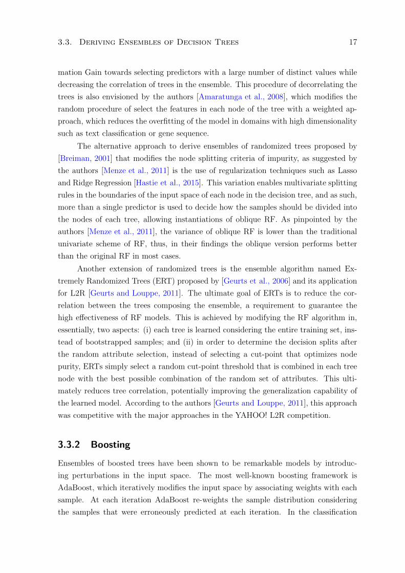
3.3. Deriving Ensembles of Decision Trees 17
mation Gain towards selecting predictors with a large number of distinct values while
decreasing the correlation of trees in the ensemble. This procedure of decorrelating the
trees is also envisioned by the authors [Amaratunga et al., 2008], which modifies the
random procedure of select the features in each node of the tree with a weighted ap-
proach, which reduces the overfitting of the model in domains with high dimensionality
such as text classification or gene sequence.
The alternative approach to derive ensembles of randomized trees proposed by
[Breiman, 2001] that modifies the node splitting criteria of impurity, as suggested by
the authors [Menze et al., 2011] is the use of regularization techniques such as Lasso
and Ridge Regression [Hastie et al., 2015]. This variation enables multivariate splitting
rules in the boundaries of the input space of each node in the decision tree, and as such,
more than a single predictor is used to decide how the samples should be divided into
the nodes of each tree, allowing instantiations of oblique RF. As pinpointed by the
authors [Menze et al., 2011], the variance of oblique RF is lower than the traditional
univariate scheme of RF, thus, in their findings the oblique version performs better
than the original RF in most cases.
Another extension of randomized trees is the ensemble algorithm named Ex-
tremely Randomized Trees (ERT) proposed by [Geurts et al., 2006] and its application
for L2R [Geurts and Louppe, 2011]. The ultimate goal of ERTs is to reduce the cor-
relation between the trees composing the ensemble, a requirement to guarantee the
high effectiveness of RF models. This is achieved by modifying the RF algorithm in,
essentially, two aspects: (i) each tree is learned considering the entire training set, ins-
tead of bootstrapped samples; and (ii) in order to determine the decision splits after
the random attribute selection, instead of selecting a cut-point that optimizes node
purity, ERTs simply select a random cut-point threshold that is combined in each tree
node with the best possible combination of the random set of attributes. This ulti-
mately reduces tree correlation, potentially improving the generalization capability of
the learned model. According to the authors [Geurts and Louppe, 2011], this approach
was competitive with the major approaches in the YAHOO! L2R competition.
3.3.2 Boosting
Ensembles of boosted trees have been shown to be remarkable models by introduc-
ing perturbations in the input space. The most well-known boosting framework is
AdaBoost, which iteratively modifies the input space by associating weights with each
sample. At each iteration AdaBoost re-weights the sample distribution considering
the samples that were erroneously predicted at each iteration. In the classification
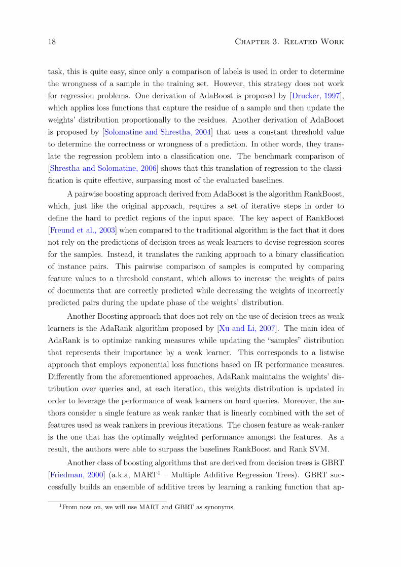
18 Chapter 3. Related Work
task, this is quite easy, since only a comparison of labels is used in order to determine
the wrongness of a sample in the training set. However, this strategy does not work
for regression problems. One derivation of AdaBoost is proposed by [Drucker, 1997],
which applies loss functions that capture the residue of a sample and then update the
weights’ distribution proportionally to the residues. Another derivation of AdaBoost
is proposed by [Solomatine and Shrestha, 2004] that uses a constant threshold value
to determine the correctness or wrongness of a prediction. In other words, they trans-
late the regression problem into a classification one. The benchmark comparison of
[Shrestha and Solomatine, 2006] shows that this translation of regression to the classi-
fication is quite effective, surpassing most of the evaluated baselines.
A pairwise boosting approach derived from AdaBoost is the algorithm RankBoost,
which, just like the original approach, requires a set of iterative steps in order to
define the hard to predict regions of the input space. The key aspect of RankBoost
[Freund et al., 2003] when compared to the traditional algorithm is the fact that it does
not rely on the predictions of decision trees as weak learners to devise regression scores
for the samples. Instead, it translates the ranking approach to a binary classification
of instance pairs. This pairwise comparison of samples is computed by comparing
feature values to a threshold constant, which allows to increase the weights of pairs
of documents that are correctly predicted while decreasing the weights of incorrectly
predicted pairs during the update phase of the weights’ distribution.
Another Boosting approach that does not rely on the use of decision trees as weak
learners is the AdaRank algorithm proposed by [Xu and Li, 2007]. The main idea of
AdaRank is to optimize ranking measures while updating the “samples” distribution
that represents their importance by a weak learner. This corresponds to a listwise
approach that employs exponential loss functions based on IR performance measures.
Differently from the aforementioned approaches, AdaRank maintains the weights’ dis-
tribution over queries and, at each iteration, this weights distribution is updated in
order to leverage the performance of weak learners on hard queries. Moreover, the au-
thors consider a single feature as weak ranker that is linearly combined with the set of
features used as weak rankers in previous iterations. The chosen feature as weak-ranker
is the one that has the optimally weighted performance amongst the features. As a
result, the authors were able to surpass the baselines RankBoost and Rank SVM.
Another class of boosting algorithms that are derived from decision trees is GBRT
[Friedman, 2000] (a.k.a, MART1 – Multiple Additive Regression Trees). GBRT suc-
cessfully builds an ensemble of additive trees by learning a ranking function that ap-
1From now on, we will use MART and GBRT as synonyms.
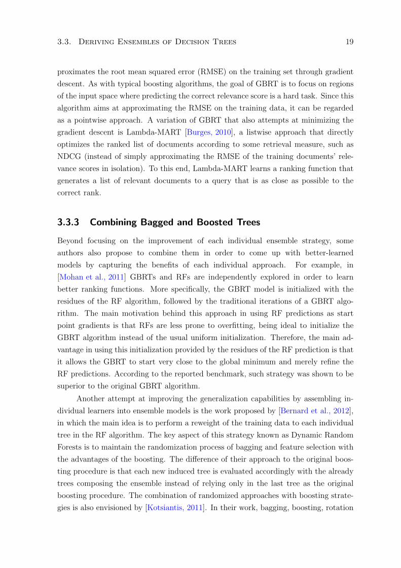
3.3. Deriving Ensembles of Decision Trees 19
proximates the root mean squared error (RMSE) on the training set through gradient
descent. As with typical boosting algorithms, the goal of GBRT is to focus on regions
of the input space where predicting the correct relevance score is a hard task. Since this
algorithm aims at approximating the RMSE on the training data, it can be regarded
as a pointwise approach. A variation of GBRT that also attempts at minimizing the
gradient descent is Lambda-MART [Burges, 2010], a listwise approach that directly
optimizes the ranked list of documents according to some retrieval measure, such as
NDCG (instead of simply approximating the RMSE of the training documents’ rele-
vance scores in isolation). To this end, Lambda-MART learns a ranking function that
generates a list of relevant documents to a query that is as close as possible to the
correct rank.
3.3.3 Combining Bagged and Boosted Trees
Beyond focusing on the improvement of each individual ensemble strategy, some
authors also propose to combine them in order to come up with better-learned
models by capturing the benefits of each individual approach. For example, in
[Mohan et al., 2011] GBRTs and RFs are independently explored in order to learn
better ranking functions. More specifically, the GBRT model is initialized with the
residues of the RF algorithm, followed by the traditional iterations of a GBRT algo-
rithm. The main motivation behind this approach in using RF predictions as start
point gradients is that RFs are less prone to overfitting, being ideal to initialize the
GBRT algorithm instead of the usual uniform initialization. Therefore, the main ad-
vantage in using this initialization provided by the residues of the RF prediction is that
it allows the GBRT to start very close to the global minimum and merely refine the
RF predictions. According to the reported benchmark, such strategy was shown to be
superior to the original GBRT algorithm.
Another attempt at improving the generalization capabilities by assembling in-
dividual learners into ensemble models is the work proposed by [Bernard et al., 2012],
in which the main idea is to perform a reweight of the training data to each individual
tree in the RF algorithm. The key aspect of this strategy known as Dynamic Random
Forests is to maintain the randomization process of bagging and feature selection with
the advantages of the boosting. The difference of their approach to the original boos-
ting procedure is that each new induced tree is evaluated accordingly with the already
trees composing the ensemble instead of relying only in the last tree as the original
boosting procedure. The combination of randomized approaches with boosting strate-
gies is also envisioned by [Kotsiantis, 2011]. In their work, bagging, boosting, rotation

20 Chapter 3. Related Work
forests and random subspace models are combined with a simple sum voting strategy
that counts the majority votes for each class of the individual algorithms. According
to the authors, the combination relying on the sum strategy showed satisfying results
when contrasted with the individual algorithms, which allowed them to conclude that
Boosting and Rotation Forests assist in regions with smaller noise, while bagging and
random subspace methods are more robust in noisy regions of the input space.
Differently from the aforementioned related works, we base ourselves in a recent
development for text classification, namely, the BROOF algorithm [Salles et al., 2015].
In their approach, a similar approach to the one of [Zhang and Xie, 2010] is used, in
which a RF machine is applied as the weak learner algorithm of the boosting meta-
algorithm. The advantages of BROOF is that the RF and boosting strategies are
tightly coupled in order to exploit their unique advantages: by exploiting out-of-bag
error estimates as well as selectively updating training weights according to out-of-bag
samples, the BROOF model is able to focus on hard-to-classify regions of the input
space, without being compromised by the boosting tendency to overfit. This ultimately
leads to competitive results when compared to the state-of-the-art algorithms. In here,
we generalize such approach specifically for L2R tasks in order to come up with better
ranking functions: we called the Generalized BROOF-L2R. As we shall see, this general
framework is flexible enough so that it can be instantiated in several ways, exploiting
distinct characteristics of the ranking tasks being addressed. In special, with this
general framework, we are able to achieve state-of-the-art results, with rankers superior
to the top-notch algorithms proposed so far in all evaluated cases.
Chapter 4
Generalized BROOF-L2R
In this chapter, we detail our proposed Generalized BROOF-L2R framework. Briefly
speaking, this framework allows the definition of learners based on the combination of
Random Forests and the Boosting meta-algorithm, in a non-trivial fashion. In doing
so, we capture the advantages of each individual algorithm to build a stronger model,
capable of maintaining the minimization of the variance by disturbing the input space
through randomization techniques such as Bagging [Breiman, 1996a]. And, with the
disturbance in the input space through manipulation of the hard regions acquired by
the boosting procedure, our instantiations might help to reduce the bias just like the
original AdaBoost proposal described in [Schapire and Freund, 2012]. Therefore, our
proposed combination of this two ML approaches can effectively help each other in
order to enhance the effectiveness of the final model and provide a better control of the
bias/variance trade-off.
As we shall see, this framework establishes a set of operations to be performed
during the boosting iterations in a well-defined order of application. The goal is to drive
the weak learners towards hard to predict regions of the underlying data representa-
tion, in order to come up with an optimized additive combination of weak learners
to form the final predictor. The extension points that we describe in this proposed
framework can produce a heterogeneous set of instantiations that typically produce
very competitive results for L2R. In the following, we present the generalized frame-
work for L2R, as well as some pointwise instantiations. Although we only describe the
most descriptive derivations in this work, it is important to stress out that the set of
derived combinations discussed here is far from exhaustive, being possible to elaborate
even better possibilities, which we will let open as future work. We first start by giving
a description of how we combine these two ML algorithms and how to make instantia-
tions by following a set of procedures. We then describe each of the instantiations that
21

22 Chapter 4. Generalized BROOF-L2R
were able to achieve statistical gains when compared to the baselines.
4.1 Framework Description
Based on the ideas of the algorithm BROOF, which was proposed by [Salles et al., 2015]
to solve text classification tasks, we here extend it in order to exploit the combination
of Random Forests and Boosting for the specific task of L2R. However, instead of
directly adapting the original algorithm to a single L2R method, we here generalize it
into an extensible framework that is flexible enough to permit a series of possible ins-
tantiations. The proposed framework named Generalized BROOF-L2R is an additive
model composed of several Random Forest models, which act as weak learners. Each
fitted model influences the final decision proportionally to its accuracy, focusing – as
the boosting iterations go by – on more complex regions of the input space, in order
to drive down the expected error. As usual in a boosting strategy, three aspects play
a key role: (i) the influence βt of each weak learner in the fitted additive model; (ii)
the strategy to update the samples distribution wmn for a document xn in query qm in
each iteration t of the boosting meta-algorithm and (iii) how to combine the individual
weak learners created in each iteration of the boosting procedure in order to enhance
the performance in terms of effectiveness of the model.
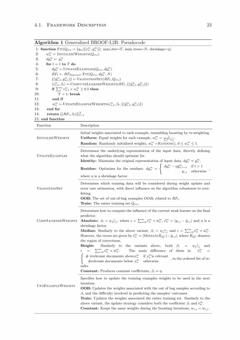
The basic structure of the framework is outlined in Algorithm 1, together with a
brief explanation of what we call its extension points – the general functions exploited
by the framework to determine how the optimization process works. There is a set of
5 general functions whose purpose is to specify the weight distribution update process,
the error estimation, and the underlying input data representation that the algorithm
should focus on minimizing. Particularly, the use of the Random Forest classifier as
a weak learner extends the range of possible instantiations of the framework, since it
enables us to come up with better error rate estimates and a more selective approach
to update the examples’ weights, through the use of the so-called out-of-bag samples.
Following the pseudo code described in this same Algorithm, we can verify that
the function Fit accepts as parameter a set of queries Qtrn = {qm, (xmn , ymn )}, each one
with its set of documents xmn with its associated graded relevance judgment ymn that
are used to build the final ensemble. The parameter max iter = T is a requirement to
identify the maximum number of rounds of boosting that must be performed in case
the heuristic used as stopping criteria is not achieved during the iterations. Finally, the
shrinkage factor η is a measure that controls the learning rate of the algorithm. This
4.1. Framework Description 23
Algorithm 1 Generalized BROOF-L2R: Pseudocode
1: function Fit(Qtrn = {qm|{xmn , ymn }}, max iter=T , num trees=N , shrinkage=η)
2: wmn = InitializeWeights(Qtrn)
3: dymn ← ymn4: for t = 1 to T do
5: dymn ←UpdateExamples(Qtrn , dymn )
6: RFt ← RFRegressor .Fit(Qtrn , dymn , N)
7: {(ymn,t, ymn,t)} ←ValidationSet(RFt, Qtrn)
8: 〈emn,t, βt〉 ←ComputeLearnerWeights(RFt, {(ymn,t, ymn,t)})9: if
∑m1 emn,t × wmn ≥ 0.5 then
10: T = t; break
11: end if
12: wmn ←UpdateExampleWeights(emn,t, βt, {(ymn,t, ymn,t)})13: end for
14: return {(RFt, βt)}|Tt=1
15: end function
Function Description
InitializeWeights
Initial weights associated to each example, resembling boosting by re-weighting.
Uniform: Equal weights for each example, wmn = 1∑m1 nm
.
Random: Randomly initialized weights, wmn =Random(), 0 ≤ wmn ≤ 1.
UpdateExamples
Determines the underlying representation of the input data, directly defining
what the algorithm should optimize for.
Identity: Maintains the original representation of input data, dymn = ymn .
Residue: Optimizes for the residues: dymn =
{dymn − ηymn,t−1 if t > 1
yi,j otherwise,
where η is a shrinkage factor.
ValidationSet
Determines which training data will be considered during weight update and
error rate estimation, with direct influence on the algorithm robustness to over-
fitting.
OOB: The set of out-of-bag examples OOBt related to RFt.
Train: The entire training set Qtrn .
CompLearnerWeights
Determines how to compute the influence of the current weak learner on the final
predictor.
Absolute: βt = η ε1−ε , where ε =
∑mi=0 e
mn × wmn , emn = |yi,j − yi,j | and η is a
shrinkage factor.
Median: Similarly to the above variant, βt = η ε1−ε and ε =
∑mi=0 e
mn × wmn .
However, the errors are given by emn = |Median(Rymn )−yi,j |, where Rymn denotes
the region of correctness.
Height: Similarly to the variants above, both βt = η ε1−ε and
ε =∑mi=0 e
mn × wmn . The main difference of them is: emn ={
# irrelevant documents abovexmn if xmn is relevant
#relevant documents below xmn otherwise, in the ordered list of re-
sults.
Constant: Produces constant coefficients, βt = η.
UpdExampleWeights
Specifies how to update the training examples weights to be used in the next
iteration.
OOB: Updates the weights associated with the out of bag samples according to
βt and the difficulty involved in predicting the samples’ outcomes.
Train: Updates the weights associated the entire training set. Similarly to the
above variant, the update strategy considers both the coefficient βt and emn .
Constant: Keeps the same weights during the boosting iterations, wi,j = wi,j .
24 Chapter 4. Generalized BROOF-L2R
learning rate is highly correlated with the number of iterations, since a small value for
η might achieve maximum effectiveness in minimizing a given loss function with a cost
of a large number of iterations, which might cause overfitting on training data. On the
other hand, choosing a large value for the learning rate η will require less iterations
to achieve the minimum local, but it might as well overpass it, which may cause the
model to lose its generalization capabilities. As seen in most boosting algorithms, the
largest variations in effectiveness by modifying this parameter occurs when minimizing
the gradient with the least square loss function.
Given the set of aforementioned parameters, the first procedure of Algorithm 1 is
the InitializeWeights function, which is responsible for the initialization of the samples
distribution that defines the importance of a document xn during the construction of
weak learners in each iteration t of the boosting procedure. There are a few ways of
initializing theses weights when starting the boosting procedure, such as Dirichlet Ran-
domization to allow a more uniform distribution by applying random values amongst
the samples, or simply using the uniform initialization, which considers that all samples
are equally important at the beginning of the boosting.
At each boosting iteration, the input data representation may be updated,
through the general function UpdateExamples. This second step defines the underly-
ing data representation that the algorithm should optimize for. The two possibilities are
to optimize for the original ground truth ymn of the input space and the second one is to
optimize for the minimization of the residues, by updating at each step the ground truth
of the samples using gradient descent. Therefore this function considerably extends the
range of possible implementations of the framework by allowing to instantiate derived
versions of the Gradient Boosting Machine [Mason et al., 2000, Hastie et al., 2009].
After defining the underlying data representation that the algorithm should optimize,
a RF regressor is built upon the set of queries Qtrn considering the current configura-
tion.
In order to evaluate the generalization capabilities of a RFt at a given iteration
t, a validation technique is applied during the creation of the model by predicting
the relevance scores y for a set of training documents given by ValidationSet. The
general function ValidationSet serves the purpose of specifying which training exam-
ples should be used during error estimation and weights update. The samples that are
used for the validation technique can be the original set of samples in the input space
or the left apart out-of-bag samples of each individual tree in the committee. The
output of this step is paramount to guide the optimization process towards hard to
classify regions of the input space. Although being of great importance to boosting
effectiveness, this focuses on hard to classify regions of the input space may also be
4.1. Framework Description 25
harmful to the optimization process, especially when dealing with noisy data. As noted
by [Freund and Schapire, 1996, Jin et al., 2003], boosting tends to increase the weights
of a few hard-to-classify examples (e.g., noisy ones). Thus, the decision boundaries may
only be suitable for those noisy regions of the input space while not necessarily general
enough for the most common examples. In order to improve robustness against such
a problem, our framework exploits an intermediary step related to how the examples
weights get updated as the boosting iterations go by. The main goal here is to provide
some mechanism to slow down overfitting as well as to provide more robust estimates
of error in order to increase the generalization power of each weak learner and to
determine how they should influence the final predictor.
The selected training examples are then used to compute both the error rate of
the model and the influence βt of the weak learner on the final model, by means of the
ComputeLearnerWeights function. This fourth (and most important) step allows
to devise the loss functions that are used to compute the influence of the current weak
learner at a given iteration t by capturing the residues of the samples selected by the
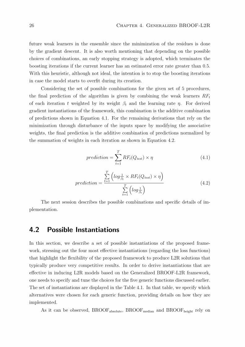
ValidationSet function. In this work, we devised 4 loss functions for the L2R context:
(i) The first one, which we named Absolute loss computes the difference in prediction
of its predicted regression value ymn to its ground truth ymn relevance judgment. (ii)
The second loss function which we call Median Region computes the median distance
of related relevant judgments samples. (iii) The third one named Height computes the
height of a document, by pushing non-relevant documents to the bottom of the ranked
list while pushing relevant ones to the top. (iv) The fourth loss function which we name
GBROOF considers constant coefficients, and therefore it relies on the minimization
of residues by using the gradient descent minimization.
Finally, the training examples’ weight distribution is updated by the function
UpdateExampleWeights. This updating process should, ideally, take into account
the generalization capability of the current weak learner RFt, as well as how hard is
to correctly predict the ranked lists of the validation examples. Validation examples
whose outcome is hard to predict by an accurate learner should influence more in the
following boosting iterations, so the updates should indicate which samples will have
a better preference in the foreseeable iterations of the boosting procedure for a given
iteration t. So far, we considered 3 approaches for updating the weights distribution.
The first one is to consider the entire training set, such that all training samples are
updated. The second updating scheme considers only the left apart samples in the
out-of-bag, which produces predictions for all samples in the training if the number
of trees is large enough, since the trees are built with bootstrapped samples with
replacement. The third variation does not update the samples in order to induce the
26 Chapter 4. Generalized BROOF-L2R
future weak learners in the ensemble since the minimization of the residues is done
by the gradient descent. It is also worth mentioning that depending on the possible
choices of combinations, an early stopping strategy is adopted, which terminates the
boosting iterations if the current learner has an estimated error rate greater than 0.5.
With this heuristic, although not ideal, the intention is to stop the boosting iterations
in case the model starts to overfit during its creation.
Considering the set of possible combinations for the given set of 5 procedures,
the final prediction of the algorithm is given by combining the weak learners RFt
of each iteration t weighted by its weight βt and the learning rate η. For derived
gradient instantiations of the framework, this combination is the additive combination
of predictions shown in Equation 4.1. For the remaining derivations that rely on the
minimization through disturbance of the inputs space by modifying the associative
weights, the final prediction is the additive combination of predictions normalized by
the summation of weights in each iteration as shown in Equation 4.2.
prediction =T∑t=1
RFt(Qtest)× η (4.1)
prediction =
T∑t=1
(log 1
βt×RFt(Qtest)× η
)T∑t=1
(log 1
βt
) (4.2)
The next session describes the possible combinations and specific details of im-
plementation.
4.2 Possible Instantiations
In this section, we describe a set of possible instantiations of the proposed frame-
work, stressing out the four most effective instantiations (regarding the loss functions)
that highlight the flexibility of the proposed framework to produce L2R solutions that
typically produce very competitive results. In order to derive instantiations that are
effective in inducing L2R models based on the Generalized BROOF-L2R framework,
one needs to specify and tune the choices for the five generic functions discussed earlier.
The set of instantiations are displayed in the Table 4.1. In that table, we specify which
alternatives were chosen for each generic function, providing details on how they are
implemented.
As it can be observed, BROOFabsolute, BROOFmedian and BROOFheight rely on

4.2. Possible Instantiations 27
InstantiationDescription
Extension Point Variation
BROOFabsolute
InitializeWeights Uniform, RandomUpdateExamples IdentityValidationSet OOB, TrainComputeLearnerWeights AbsoluteUpdateExampleWeights OOB, Train
BROOFmedian
InitializeWeights Uniform, RandomUpdateExamples IdentityValidationSet OOB, TrainComputeLearnerWeights MedianUpdateExampleWeights OOB, Train
BROOFheight
InitializeWeights Uniform & RandomUpdateExamples IdentityValidationSet OOB, TrainComputeLearnerWeights HeightUpdateExampleWeights OOB, Train
BROOFgradient
InitializeWeights Uniform & RandomUpdateExamples ResidueValidationSet OOB, TrainComputeLearnerWeights ConstantUpdateExampleWeights Constant, OOB
Table 4.1: Generalized BROOF-L2R: Possible instantiations.
the use of out-of-bag samples or the whole set of training samples in order to drive
the weak learners of the boosting meta-algorithm further on hard to predict regions
of the input space. Such samples can be explored when estimating the weak learners’
error rate through out-of-bag or as usual in the original boosting procedure assessing
the errors to measure the residues through a loss function using the training set. It
is worth to mention that, as the size of the data grows, using the training data is too
optimistic, since the same data that was used to train the model is used as a measure
of error. By using the out-of-bag samples we are able to produce better error estimates
in large collections, being more effective and efficient, since the out-of-bag samples
constitute an independent set of samples that was left apart during the construction
of the model. By doing so, we are able to better approximate the expected error
rate of the learner with a more reliable measure than the usual training error rate
[Breiman, 1996b, Salles et al., 2015, de Sa et al., 2016].
In addition, the validation samples estimates are used to identify the weights’
distribution that should be applied on following iterations of the procedure, which
allows the model to focus on hard to predict regions of the input space. We hypothesize
that such selective update strategy can slow down the algorithm’s tendency to overfit
in real large-scale collections. The major difference amongst our instantiations is the
restriction on how each weak-learner influences the final predictor. To better clarify
the instantiations, we outline the specifics of each instantiation in the pseudocode of

28 Chapter 4. Generalized BROOF-L2R
Algorithms 2 to 5 along with a set of figures that represent how the loss functions work
upon the samples.
As we see in Table 4.1, for all instantiations, we derived models considering ran-
dom initialization of the samples distribution weights using Dirichlet Randomization,
which allows uniform random values between [0, 1], and the uniform initialization,
which considers that all samples are equivalent and equally weighted in the first itera-
tion. The three first instances BROOFabsolute, BROOFmedian and BROOFheight set the
configuration for the procedure UpdateExamples to optimize for the original ground
truth of samples, therefore, the instances use boosting by re-weighting. This is differ-
ent for BROOFgradient that minimizes the residue in each boosting iteration through
gradient descent. All derivations were validated with training and out-of-bag samples.
The specific details of the first instantiation are shown in Algorithm 2 with a
visual representation of the loss function in Figure 4.1. In that figure, it is considered
that the maximum relevance judgment is 4 for completely relevant documents while
the representation for non-relevant documents is 0. Let us also consider that each point
is the prediction of an RF model for a given document chosen during the validation
procedure (e.g.: out-of-bag document), where the red ones stand for non-relevant docu-
ments (ground truth equals 0) and the blue ones are relevant documents (ground truth
equals 4). The absolute regression loss computes the absolute value of the prediction
|ymn − ymn | for those samples, and then proportionally updates the weights’ distribution
according to this residue. As we can observe in this figure, all samples weights are
updated regardless of the position that they occupy in the ranking for a given query
Algorithm 2 BROOFabsolute: Pseudocode
1: function Fit({(qi, {xi,j, yi,j}|mij=1}, M , N , η)
2: wi,j = 1∑i,j mi,j
3: x′i,j ← yi,j4: for each t = 1 to M do5: x′i,j ← xi,j6: RFt ← RFRegressor .Fit({(x′i,j, yi,j)}, N)7: {(yti,j, yti,j)} ← RFt.OOB8: eti,j ← |yi,j − yi,j|9: ε←
∑i,j e
ti,jwi,j
10: βt ← η ε1−ε
11: if ε ≥ 0.5 t = T; break
12: wi,j ← wi,jβ1−eti,jt
13: end for14: return {(RFt, βt)}|Mt=1
15: end function
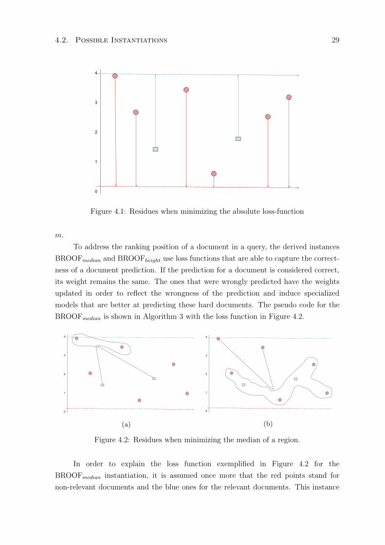
4.2. Possible Instantiations 29
4
3
2
1
0
Figure 4.1: Residues when minimizing the absolute loss-function
m.
To address the ranking position of a document in a query, the derived instances
BROOFmedian and BROOFheight use loss functions that are able to capture the correct-
ness of a document prediction. If the prediction for a document is considered correct,
its weight remains the same. The ones that were wrongly predicted have the weights
updated in order to reflect the wrongness of the prediction and induce specialized
models that are better at predicting these hard documents. The pseudo code for the
BROOFmedian is shown in Algorithm 3 with the loss function in Figure 4.2.
4
3
2
1
0
(a)
4
3
2
1
0
(b)
Figure 4.2: Residues when minimizing the median of a region.
In order to explain the loss function exemplified in Figure 4.2 for the
BROOFmedian instantiation, it is assumed once more that the red points stand for
non-relevant documents and the blue ones for the relevant documents. This instance

30 Chapter 4. Generalized BROOF-L2R
of the framework considers regions of the input space that define the “importance” of
a document. Each region is defined as the amount of samples of each individual an-
notated relevance judgment. Therefore, for a multi-relevance judgment scenario with
5 relevance judgments, the loss function would divide the input space into 5 levels, in
which in the perfect ranking, each level would contain only documents that are really
alike in terms of importance (i.e: the same annotated relevance judgment).
For the sake of our argument, let us suppose that a given query, as shown in
Figure 4.2, only contains samples with relevance judgments 4 (relevant) and 0 (non-
relevant). Thus, the input space is divided into two levels. In the perfect ranking,
the topmost level would contain two documents that are relevant, and the second level
would contain the other six, non-relevant documents. However, as we can see in Figure
4.2a, the two topmost documents are irrelevant, with two relevant documents hanging
in the middle of the non-relevant ones. Taking this into consideration, the two relevant
documents and the two top most, non-relevant documents should be swapped in order
to get the perfect ranking. This is done by re-weighting the weights’ distribution for
these samples in the wrong region of the input space. These samples are updated with
the absolute difference of the ground truth of those samples with the median of the
samples in its correct region |Median(Rymn )− ymn |. For example, in Figure 4.2a, the two
relevant documents have their weights updated with the difference of their regression
value score to the median of the circled region containing the topmost, non-relevant
documents. In Figure 4.2b the two topmost non-relevant documents are updated with
the difference of its regression value with the median of its correct region, which is
Algorithm 3 BROOFmedian: Pseudocode
1: function Fit({(qi, {xi,j, yi,j}|mij=1}, M , N , η)
2: wi,j = 1∑i,j mi,j
3: x′i,j ← yi,j4: for each t = 1 to M do5: x′i,j ← xi,j6: RFt ← RFRegressor .Fit({(x′i,j, yi,j)}, N)7: {(yti,j, yti,j)} ← RFt.OOB8: eti,j ← Median(pos(yi,j)− pos(yi,j))9: ε←
∑i,j e
ti,jwi,j
10: βt ← η ε1−ε
11: if ε ≥ 0.5 break
12: wi,j ← wi,jβ1−eti,jt
13: end for14: return {(RFt, βt)}|Mt=1
15: end function
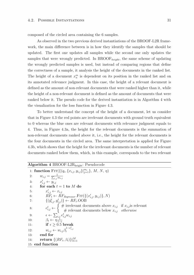
4.2. Possible Instantiations 31
composed of the circled area containing the 6 samples.
As observed in the two previous derived instantiations of the BROOF-L2R frame-
work, the main difference between is in how they identify the samples that should be
updated. The first one updates all samples while the second one only updates the
samples that were wrongly predicted. In BROOFheight, the same scheme of updating
the wrongly predicted samples is used, but instead of comparing regions that define
the correctness of a sample, it analysis the height of the documents in the ranked list.
The height of a document xmn is dependent on its position in the ranked list and on
its annotated relevance judgment. In this case, the height of a relevant document is
defined as the amount of non-relevant documents that were ranked higher than it, while
the height of a non-relevant document is defined as the amount of documents that were
ranked below it. The pseudo code for the derived instantiation is in Algorithm 4 with
the visualization for the loss function in Figure 4.3.
To better understand the concept of the height of a document, let us consider
that in Figure 4.3 the red points are irrelevant documents with ground truth equivalent
to 0 whereas the blue ones are relevant documents with relevance judgment equals to
4. Thus, in Figure 4.3a, the height for the relevant documents is the summation of
non-relevant documents ranked above it, i.e., the height for the relevant documents is
the four documents in the circled area. The same interpretation is applied for Figure
4.3b, which shows that the height for the irrelevant documents is the number of relevant
documents ranked below them, which, in this example, corresponds to the two relevant
Algorithm 4 BROOF-L2Rheight: Pseudocode
1: function Fit({(qi, {xi,j, yi,j}|mij=1}, M , N , η)
2: wi,j = 1∑i,j mi,j
3: x′i,j ← yi,j4: for each t = 1 to M do5: x′i,j ← xi,j6: RFt ← RFRegressor .Fit({(x′i,j, yi,j)}, N)7: {(yti,j, yti,j)} ← RFt.OOB
8: eti,j ←{
# irrelevant documents above xi,j if xi,jis relevant# relevant documents below xi,j otherwise
9: ε←∑
i,j eti,jwi,j
10: βt ← η ε1−ε
11: if ε ≥ 0.5 break
12: wi,j ← wi,jβ1−eti,jt
13: end for14: return {(RFt, βt)}|Mt=1
15: end function
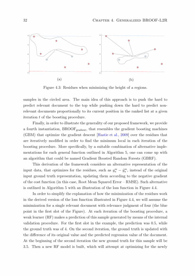
32 Chapter 4. Generalized BROOF-L2R
4
3
2
1
0
(a)
4
3
2
1
0
(b)
Figure 4.3: Residues when minimizing the height of a regions.
samples in the circled area. The main idea of this approach is to push the hard to
predict relevant document to the top while pushing down the hard to predict non-
relevant documents proportionally to its current position in the ranked list at a given
iteration t of the boosting procedure.
Finally, in order to illustrate the generality of our proposed framework, we provide
a fourth instantiation, BROOFgradient, that resembles the gradient boosting machines
(GBM) that optimize the gradient descent [Hastie et al., 2009] over the residues that
are iteratively modified in order to find the minimum local in each iteration of the
boosting procedure. More specifically, by a suitable combination of alternative imple-
mentations for each general function outlined in Algorithm 5, one can come up with
an algorithm that could be named Gradient Boosted Random Forests (GBRF).
This derivation of the framework considers an alternative representation of the
input data, that optimizes for the residues, such as ymn − ymn , instead of the original
input ground truth representation, updating them according to the negative gradient
of the cost function (in this case, Root Mean Squared Error – RMSE). Such alternative
is outlined in Algorithm 5 with an illustration of the loss function in Figure 4.4.
In order to simplify the explanation of how the minimization of the residues work
in the derived version of the loss function illustrated in Figure 4.4, we will assume the
minimization for a single relevant document with relevance judgment of four (the blue
point in the first slot of the Figure). At each iteration of the boosting procedure, a
weak learner (RF) makes a prediction of this sample generated by means of the internal
validation procedure. For the first slot in the example, the prediction was 0.5, while
the ground truth was of 4. On the second iteration, the ground truth is updated with
the difference of its original value and the predicted regression value of the document.
At the beginning of the second iteration the new ground truth for this sample will be
3.5. Then a new RF model is built, which will attempt at optimizing for the newly
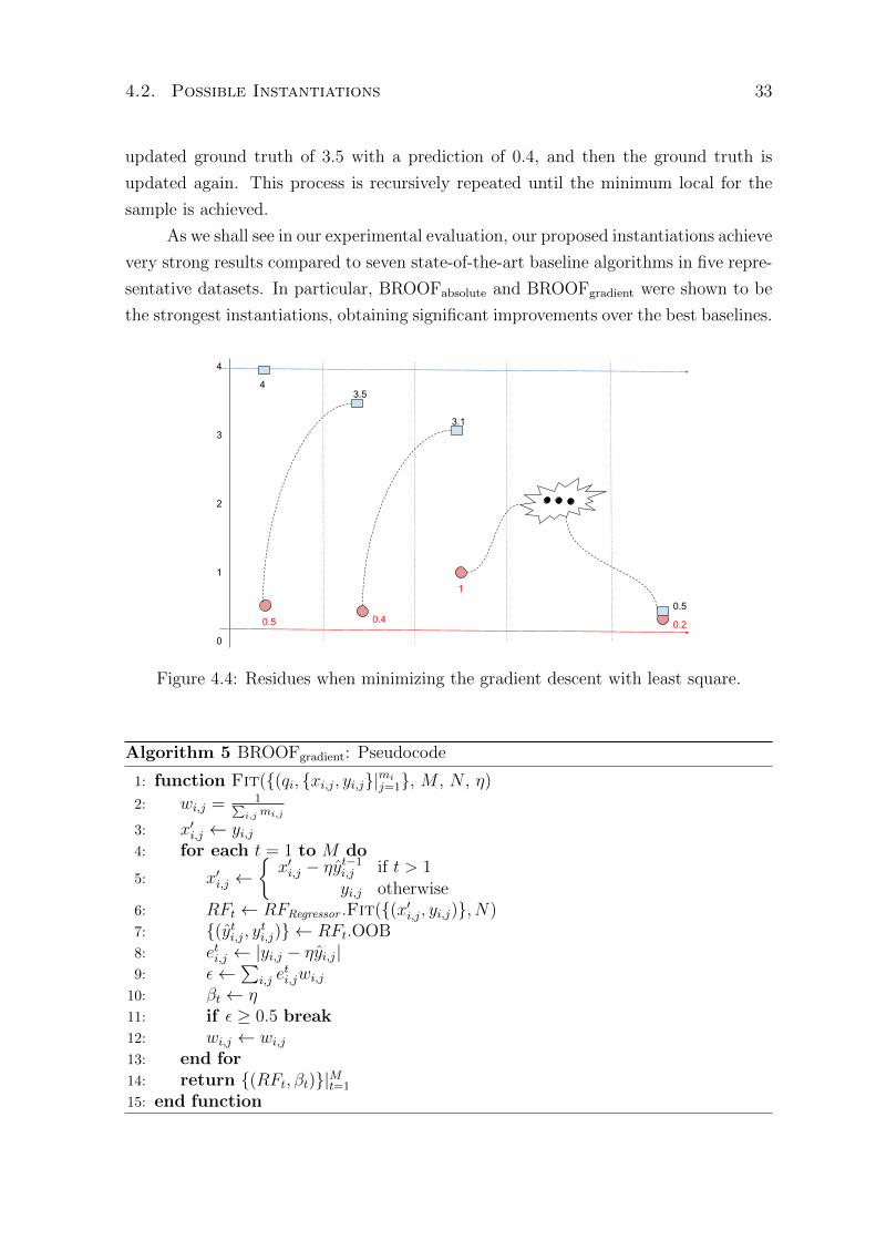
4.2. Possible Instantiations 33
updated ground truth of 3.5 with a prediction of 0.4, and then the ground truth is
updated again. This process is recursively repeated until the minimum local for the
sample is achieved.
As we shall see in our experimental evaluation, our proposed instantiations achieve
very strong results compared to seven state-of-the-art baseline algorithms in five repre-
sentative datasets. In particular, BROOFabsolute and BROOFgradient were shown to be
the strongest instantiations, obtaining significant improvements over the best baselines.
4
3
2
1
0
4
0.5 0.4
1
0.2
0.5
3.5
3.1
Figure 4.4: Residues when minimizing the gradient descent with least square.
Algorithm 5 BROOFgradient: Pseudocode
1: function Fit({(qi, {xi,j, yi,j}|mij=1}, M , N , η)
2: wi,j = 1∑i,j mi,j
3: x′i,j ← yi,j4: for each t = 1 to M do
5: x′i,j ←{x′i,j − ηyt−1i,j if t > 1
yi,j otherwise6: RFt ← RFRegressor .Fit({(x′i,j, yi,j)}, N)7: {(yti,j, yti,j)} ← RFt.OOB8: eti,j ← |yi,j − ηyi,j|9: ε←
∑i,j e
ti,jwi,j
10: βt ← η11: if ε ≥ 0.5 break12: wi,j ← wi,j13: end for14: return {(RFt, βt)}|Mt=1
15: end function


Chapter 5
Experimental Protocol and Evaluation
This chapter describes an extensive set of experiments in well-known L2R benchmarks.
In the following, we describe the characteristics of the datasets, baseline algorithms
and the experimental protocol and setup.
5.1 Datasets
The corpora we use to evaluate the effectiveness of the studied algorithms are freely
available online for scientific purposes. Such datasets can be divided into two groups
considering the relevance judgments and their sizes. The two largest datasets contains
{query, document} pairs with five relevance judgment levels, ranging from 0 (com-
pletely irrelevant) to 4 (highly relevant). In this group we have the WEB10K1 dataset
that consists of a subset of 10,000 random queries extracted from the web search engine
Microsoft Bing. The second largest collection, YAHOO! Webscope Learning to Rank
Challenge2, contains 6,330 queries. In contrast to the Microsoft collection, which is
partitioned into 5 folds for cross-validation purposes (3 partitions used for training, 1
for validation and 1 for the test in each one of the 5 folds), the YAHOO! Webscope
contains a single fold that splits the data into three subsets: training and validation
containing 1,266 queries each and test containing 3,798 queries.
The second group of datasets corresponds to the well-known LETOR 3.0 Topic
Distillation tasks (TD) (a.k.a., informational queries), of the Web track in the Text
Retrieval Conference 2003 (TD2003) and 2004 (TD2004)3. These datasets contain
1https://www.microsoft.com/en-us/research/project/mslr/2https://webscope.sandbox.yahoo.com/3http://research.microsoft.com/en-us/um/beijing/projects/letor/
35
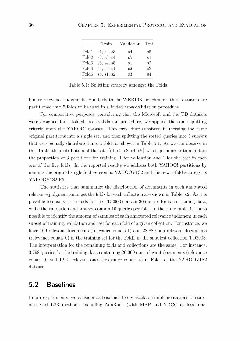
36 Chapter 5. Experimental Protocol and Evaluation
Train Validation Test
Fold1 s1, s2, s3 s4 s5Fold2 s2, s3, s4 s5 s1Fold3 s3, s4, s5 s1 s2Fold4 s4, s5, s1 s2 s3Fold5 s5, s1, s2 s3 s4
Table 5.1: Splitting strategy amongst the Folds
binary relevance judgments. Similarly to the WEB10K benchmark, these datasets are
partitioned into 5 folds to be used in a folded cross-validation procedure.
For comparative purposes, considering that the Microsoft and the TD datasets
were designed for a folded cross-validation procedure, we applied the same splitting
criteria upon the YAHOO! dataset. This procedure consisted in merging the three
original partitions into a single set, and then splitting the sorted queries into 5 subsets
that were equally distributed into 5 folds as shown in Table 5.1. As we can observe in
this Table, the distribution of the sets {s1, s2, s3, s4, s5} was kept in order to maintain
the proportion of 3 partitions for training, 1 for validation and 1 for the test in each
one of the five folds. In the reported results we address both YAHOO! partitions by
naming the original single fold version as YAHOOV1S2 and the new 5-fold strategy as
YAHOOV1S2-F5.
The statistics that summarize the distribution of documents in each annotated
relevance judgment amongst the folds for each collection are shown in Table 5.2. As it is
possible to observe, the folds for the TD2003 contain 30 queries for each training data,
while the validation and test set contain 10 queries per fold. In the same table, it is also
possible to identify the amount of samples of each annotated relevance judgment in each
subset of training, validation and test for each fold of a given collection. For instance, we
have 169 relevant documents (relevance equals 1) and 28,889 non-relevant documents
(relevance equals 0) in the training set for the Fold1 in the smallest collection TD2003.
The interpretation for the remaining folds and collections are the same. For instance,
3,798 queries for the training data containing 26,069 non-relevant documents (relevance
equals 0) and 1,921 relevant ones (relevance equals 4) in Fold1 of the YAHOOV1S2
dataset.
5.2 Baselines
In our experiments, we consider as baselines freely available implementations of state-
of-the-art L2R methods, including AdaRank (with MAP and NDCG as loss func-
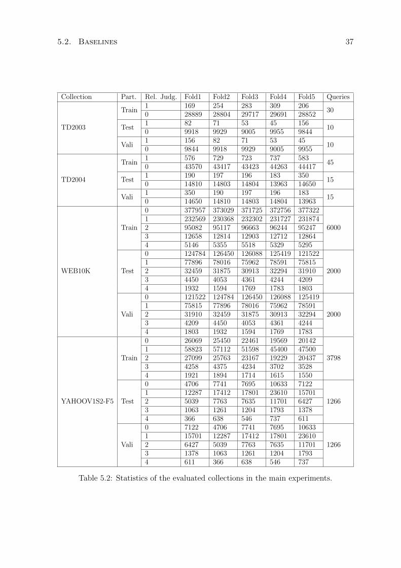
5.2. Baselines 37
Collection Part. Rel. Judg. Fold1 Fold2 Fold3 Fold4 Fold5 Queries
TD2003
Train1 169 254 283 309 206
300 28889 28804 29717 29691 28852
Test1 82 71 53 45 156
100 9918 9929 9005 9955 9844
Vali1 156 82 71 53 45
100 9844 9918 9929 9005 9955
TD2004
Train1 576 729 723 737 583
450 43570 43417 43423 44263 44417
Test1 190 197 196 183 350
150 14810 14803 14804 13963 14650
Vali1 350 190 197 196 183
150 14650 14810 14803 14804 13963
WEB10K
Train
0 377957 373029 371725 372756 377322
60001 232569 230368 232302 231727 2318742 95082 95117 96663 96244 952473 12658 12814 12903 12712 128644 5146 5355 5518 5329 5295
Test
0 124784 126450 126088 125419 121522
20001 77896 78016 75962 78591 758152 32459 31875 30913 32294 319103 4450 4053 4361 4244 42094 1932 1594 1769 1783 1803
Vali
0 121522 124784 126450 126088 125419
20001 75815 77896 78016 75962 785912 31910 32459 31875 30913 322943 4209 4450 4053 4361 42444 1803 1932 1594 1769 1783
YAHOOV1S2-F5
Train
0 26069 25450 22461 19569 20142
37981 58823 57112 51598 45400 475002 27099 25763 23167 19229 204373 4258 4375 4234 3702 35284 1921 1894 1714 1615 1550
Test
0 4706 7741 7695 10633 7122
12661 12287 17412 17801 23610 157012 5039 7763 7635 11701 64273 1063 1261 1204 1793 13784 366 638 546 737 611
Vali
0 7122 4706 7741 7695 10633
12661 15701 12287 17412 17801 236102 6427 5039 7763 7635 117013 1378 1063 1261 1204 17934 611 366 638 546 737
Table 5.2: Statistics of the evaluated collections in the main experiments.
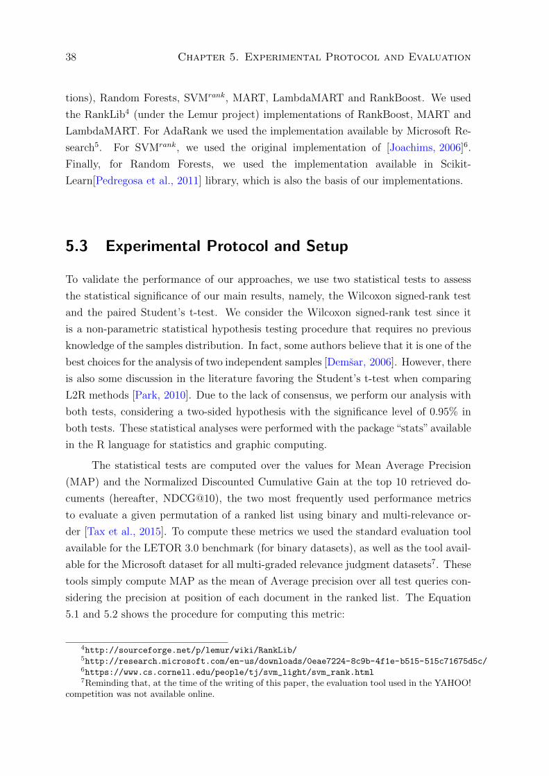
38 Chapter 5. Experimental Protocol and Evaluation
tions), Random Forests, SVMrank, MART, LambdaMART and RankBoost. We used
the RankLib4 (under the Lemur project) implementations of RankBoost, MART and
LambdaMART. For AdaRank we used the implementation available by Microsoft Re-
search5. For SVMrank, we used the original implementation of [Joachims, 2006]6.
Finally, for Random Forests, we used the implementation available in Scikit-
Learn[Pedregosa et al., 2011] library, which is also the basis of our implementations.
5.3 Experimental Protocol and Setup
To validate the performance of our approaches, we use two statistical tests to assess
the statistical significance of our main results, namely, the Wilcoxon signed-rank test
and the paired Student’s t-test. We consider the Wilcoxon signed-rank test since it
is a non-parametric statistical hypothesis testing procedure that requires no previous
knowledge of the samples distribution. In fact, some authors believe that it is one of the
best choices for the analysis of two independent samples [Demsar, 2006]. However, there
is also some discussion in the literature favoring the Student’s t-test when comparing
L2R methods [Park, 2010]. Due to the lack of consensus, we perform our analysis with
both tests, considering a two-sided hypothesis with the significance level of 0.95% in
both tests. These statistical analyses were performed with the package “stats” available
in the R language for statistics and graphic computing.
The statistical tests are computed over the values for Mean Average Precision
(MAP) and the Normalized Discounted Cumulative Gain at the top 10 retrieved do-
cuments (hereafter, NDCG@10), the two most frequently used performance metrics
to evaluate a given permutation of a ranked list using binary and multi-relevance or-
der [Tax et al., 2015]. To compute these metrics we used the standard evaluation tool
available for the LETOR 3.0 benchmark (for binary datasets), as well as the tool avail-
able for the Microsoft dataset for all multi-graded relevance judgment datasets7. These
tools simply compute MAP as the mean of Average precision over all test queries con-
sidering the precision at position of each document in the ranked list. The Equation
5.1 and 5.2 shows the procedure for computing this metric:
4http://sourceforge.net/p/lemur/wiki/RankLib/5http://research.microsoft.com/en-us/downloads/0eae7224-8c9b-4f1e-b515-515c71675d5c/6https://www.cs.cornell.edu/people/tj/svm_light/svm_rank.html7Reminding that, at the time of the writing of this paper, the evaluation tool used in the YAHOO!
competition was not available online.
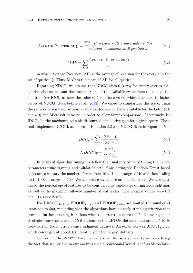
5.3. Experimental Protocol and Setup 39
AveragePrecision(q) =
∑ki=1 Precision× Relevance judgment@i
relevant documents until position k(5.1)
MAP =∑q∈Q
AveragePrecision(q)
|Q|, (5.2)
in which Average Precision (AP) is the average of precision for the query q in the
set of queries Q. Thus, MAP is the mean of AP for all queries.
Regarding NDCG, we assume that NDCG@k is 0 (zero) for empty queries, i.e.,
queries with no relevant documents. Some of the available evaluations tools (e.g., the
one from YAHOO!) assume the value of 1 for these cases, which may lead to higher
values of NDCG [Busa-Fekete et al., 2013]. We chose to standardize this issue, using
the same criterion used by most evaluation tools, e.g., those available for the Letor (3.0
and 4.0) and Microsoft datasets, in order to allow fairer comparisons. Accordingly, let
IDCGp be the maximum possible discounted cumulative gain for a given query. These
tools implement DCG@k as shown in Equation 5.3 and NDCG@k as in Equation 5.4:
DCGp =
p∑i=1
2reli − 1
log2(i+ 1)(5.3)
NDCG@p =DCGp
IDCGp
. (5.4)
In terms of algorithm tuning, we follow the usual procedure of tuning the hyper-
parameters using training and validation sets. Considering the Random Forest based
approaches we vary the number of trees from 10 to 100 in ranges of 10 and then scaling
up to 1000 in ranges of 100. We achieved convergence around 300 trees. We also opti-
mized the percentage of features to be considered as candidates during node splitting,
as well as the maximum allowed number of leaf nodes. The optimal values were 0.3
and 100, respectively.
For BROOFabsolute, BROOFmedian and BROOFheight, we limited the number of
iterations to 500, reminding that the algorithms have an early stopping criterion that
prevents further boosting iterations when the error rate exceeds 0.5. On average, our
strategies converge at about 15 iterations on the LETOR datasets, and around 5 to 10
iterations on the multi-relevance judgment datasets. An exception was BROOFgradient
which converged at about 100 iterations for the largest datasets.
Concerning the SVMrank baseline, we favored the use of a linear kernel considering
the fact that we verified in our analysis that a polynomial kernel is infeasible on large

40 Chapter 5. Experimental Protocol and Evaluation
scale benchmarks such as WEB10K. The cost parameter C was calibrated using the
training and validation sets with the explored values: 0.001, 0.01, 0.1, 1, 10, 100
and 1000. For the boosting methods Mart and LambdaMART, we tuned, always
considering the validation set, the number of iterations ranging from one to a hundred,
with a step of 1, and then scaling it up to 1000 iterations, with steps of 100. For the
shrinkage factor of the predictive models, we tested the values of 0.025, 0.05, 0.075 and
0.1. The best found values for the MART and LambdaMART were ensembles of 1000
trees with shrinkage factor η of 0.1. For the AdaRankMAP , AdaRankNDCG@5 and for
the RankBoost algorithm, similar procedures were performed in the validation set to
configure the number of iterations.
Finally, we performed 5, 10 and 30 runs of the 5-fold cross validation procedure for
WEB10K, YAHOO! and LETOR datasets, respectively. The differences in the number
of repetitions are due to the size of the datasets and the need to properly address the
variance of the results. The reported results on Tables 6.1 and 6.2 are the average of
all these runs, being the statistical tests applied to these results.
Chapter 6
Experimental Results
In this chapter, we report the results of our approaches over state-of-the-art baselines
in 5 known L2R datasets. We first present the benchmark comparisons that demon-
strate the benefits of our instantiations over the evaluated baselines, then we present
a convergence analysis of the strongest instantiations in the most representative col-
lections. We also address the issue of the generalization capabilities of our approaches
under a constrained number of training samples, which shows that our approaches are
capable of achieving the strongest results with smaller percentages of training data.
In the sequence, we investigate the advantages of wisely choosing the correct way of
setting the ValidationSet function of Algorithm 1. Finally, we conclude the chapter
with a discussion of the main factors that influence the proposed instantiations with
an analysis design that shows the advances of our induced loss functions for L2R.
6.1 Benchmark Comparisons
In this section we analyze our proposals in terms of effectiveness, comparing the derived
instances of the framework to 7 baseline algorithms in 5 datasets. The main results
containing the statistical significance of 0.95% of confidence using the T-student and
the Wilcoxon Signed Rank Sum hypothesis test are reported on Table 6.1 considering
the Mean Average Precision (MAP). Table 6.2 shows the outcomes for the Normalized
Discounted Cumulative Gain (NDCG@10). To make the interpretation of the results
easier to understand, the values in red boxes are the stronger baselines, while the
ones with an underline are the strongest baselines that tied with at least one of our
instantiations (which is also underlined in the case of a tie) in both statistical hypothesis
tests. The values in the green box represent our strongest instantiation. The starred
values (?) means that the derived instantiation of the framework was able to achieve
41

42 Chapter 6. Experimental Results
statistical significance with the Wilcoxon test, while the signed plus values (+) represent
statistical gains with the statistical analysis of the T-student test.
6.1.1 Mean Average Precision – MAP
We start by considering the MAP metric on Table 6.1. As it is possible to observe,
the MAP results show that in general our proposed framework outperforms or ties
with the strongest baselines in all collections. More specifically, the BROOFabsolute
instantiation obtained the highest value in MAP with gain regarding the statistical
hypothesis test Wilcoxon with of 0.288 of effectiveness against 0.278 for the strongest
baseline – RF – in the collection TD2003. We can also note for this collection that the
remaining derived instantiations of the framework were able to achieve similar gains,
with BROOFmedian outperforming the strongest baseline with the T-student test and
BROOFheight successfully bypassing the RF baseline in both statistical tests. As it is
possible to observe, BROOFgradient ties with the strongest baseline.
Considering the collection TD2004, the ensemble model BROOFabsolute was con-
sidered the top performer amongst the proposed solutions, being tied with the strongest
baseline RankBoost. Although not explicitly shown in this table, it is worth to
mention that all four of our instantiations achieve statistical gains by overcoming
all other baselines in both Wilcoxon and T-Student test. Regarding the WEB10K
dataset, we observe the same patterns, which shows that our approaches BROOFabsolute,
BROOFmedian and BROOFheight were also able to achieve statistical gains over distinct
baselines with strong evidence for the BROOFgradient as the leading winner model, since
AlgorithmDatasets
TD2003 TD2004 WEB10K YAHOOV1S2 YAHOOV1S2-5F
Mart 0.192633 0.193744 0.352491 0.559721 0.568821LambdaMart 0.165181 0.169605 0.350263 0.5545 0.563694RF 0.278644 0.2522 0.337702 0.563355 0.559019RankBoost 0.235189 0.255467 0.316201 0.544887 0.547524AdaRank-MAP 0.2003 0.196801 0.294792 0.413846 0.480190Adarank-NDCG 0.121672 0.132435 0.304359 0.540243 0.538514SVM-Rank 0.257490 0.220392 0.324552 0.544887 0.551333
BROOFabsolute 0.288039+ 0.263288 0.342437 0.565486∗+ 0.563729BROOFmedian 0.282427∗ 0.259941 0.347665 0.567696∗+ 0.567284BROOFheight 0.285937∗+ 0.259058 0.340340 0.564774∗+ 0.557727BROOFgradient 0.280634 0.252342 0.36251∗+ 0.572918∗+ 0.57656∗+
‘∗’: statistical significance according to Wilcoxon Test‘+’: statistical significance according to Student’s t-test
‘n’: statistically tied results considering both tests
Table 6.1: Mean Average Precision (MAP): Obtained results.
6.1. Benchmark Comparisons 43
it was able to overcome the results of the strongest baseline MART in both statistical
hypothesis tests.
Finally, in the YAHOOV1S2 dataset, the strongest baseline was the algorithm RF,
which showed to be inferior to all four of our proposed algorithms in both statistical
hypothesis tests. As noted on the Table, it is clear that BROOFgradient is the winner
derivation of our framework in both YAHOO! collections with gains in both statistical
hypothesis tests. In sum, according to the MAP metric, our results clearly show that
the proposed instantiations of the Generalized BROOF-L2R framework produce very
competitive results as the best algorithm is superior in the majority of cases, tying in
a few others – a very significant result.
6.1.2 Normalized Discounted Cumulative Gain – NDCG
Turning our attention to the NDCG results reported on Table 6.2, a similar behavior
can be observed: our proposed instantiations are no worse than the strongest baselines
in all cases, being superior in the majority of cases. Considering the TD2003 and
TD2004 datasets, our solutions were no worse than any baseline, being statistically
tied with the strongest one (RF, in both cases). For the respective collections, our
instantiations BROOFgradient and BROOFabsolute were favored in the respective dataset
obtaining the highest average value of NDCG.
The results for WEB10K show that BROOFgradient is able to surpass the strongest
baseline LambdaMart in both statistical hypothesis tests, and the same observation of
the MAP in this collection is applied in the remaining derivations of the framework,
AlgorithmDatasets
TD2003 TD2004 WEB10K YAHOOV1S2 YAHOOV1S2-5F
Mart 0.271274 0.263926 0.4404 0.703757 0.714763LambdaMart 0.224536 0.237338 0.445437 0.69619 0.706287RF 0.36346 0.350582 0.424498 0.703139 0.702384RankBoost 0.31613 0.33399 0.397071 0.682478 0.681796AdaRank-MAP 0.271921 0.281035 0.35732 0.51767 0.607867AdaRank-NDCG 0.166241 0.182031 0.385761 0.66309 0.664115SVM-Rank 0.344177 0.303471 0.399902 0.682478 0.691064
BROOFabsolute 0.360802 0.358146 0.434964 0.70633 0.706954BROOFmedian 0.36798 0.350466 0.436284 0.708538+ 0.709148BROOFheight 0.368195 0.355356 0.42882 0.70383 0.701985BROOFgradient 0.368695 0.348532 0.456081∗+ 0.717271∗+ 0.725129∗+
‘∗’: statistical significance according to Wilcoxon Test‘+’: statistical significance according to Student’s t-test
‘n’: statistically tied results considering both tests
Table 6.2: Normalized Discounted Cumulative Gain (NDCG@10): Obtained results.

44 Chapter 6. Experimental Results
noting that they were able to achieve statistically significant gains over the remaining
individual baselines.
Furthermore, BROOFmedian was also superior to the best baseline ensemble
MART in the YAHOOV1S2 dataset according to the Student’s t-test. For the same
collection, BROOFgradient surpassed the strongest baseline in both Wilcoxon and T-
Student hypothesis tests. The remaining derivations BROOFabsolute and BROOFheight
tied with the MART algorithm, which highlights once more the effectiveness of the
proposed approaches, since we always surpass or tie with all baselines. Finally for the
multi-folded version YAHOOV1S2-F5 dataset, the instantiation BROOFgradient show
its potential by surpassing the strongest baseline in both employed statistical tests.
6.2 Behavioral Analysis
We now turn our attention to some behavioral aspects of our algorithms namely conver-
gence rate, learning effectiveness towards optimizing training data and validation ana-
lysis. We start by contrasting the convergence rate of the boosting baseline approaches
with our best derivation in the largest collections. Then we discuss the effectiveness of
the algorithms in generalizing its predictive abilities under constrained training data.
Finally, we address the use of training or out-of-bag samples in order to update the
samples distribution towards hard to predict regions of the input space.
6.2.1 Convergence Rate
In order to better understand the convergence rate of our proposals, we provide an
empirical evaluation of our most effective solution BROOFgradient, by analyzing the
obtained NDCG@10 as we vary the number of rounds of boosting. We here focus on
contrasting the results on the three largest datasets: WEB10K, YAHOOV1S2, and its
multi-fold version YAHOOV1S2-F5. The findings for this experiment can be found in
Figure 6.1.
As can be observed, BROOFgradient share a similar behavior with three explored
boosting algorithms, namely, MART, RankBoost and AdaRank-NDCG for all collec-
tions. The four algorithms show fast convergence rates, and differ in two key aspects:
(i) our approach is able to achieve significantly better results at the initial boosting
iterations, which leads to the second aspect (ii) that our BROOFgradient converges to
a higher asymptote than the other algorithms. Therefore it was able to surpass the
strongest baseline MART with only a few rounds of boosting. On the other hand, the
convergence rate of LambdaMART was significantly slower than the convergence rate
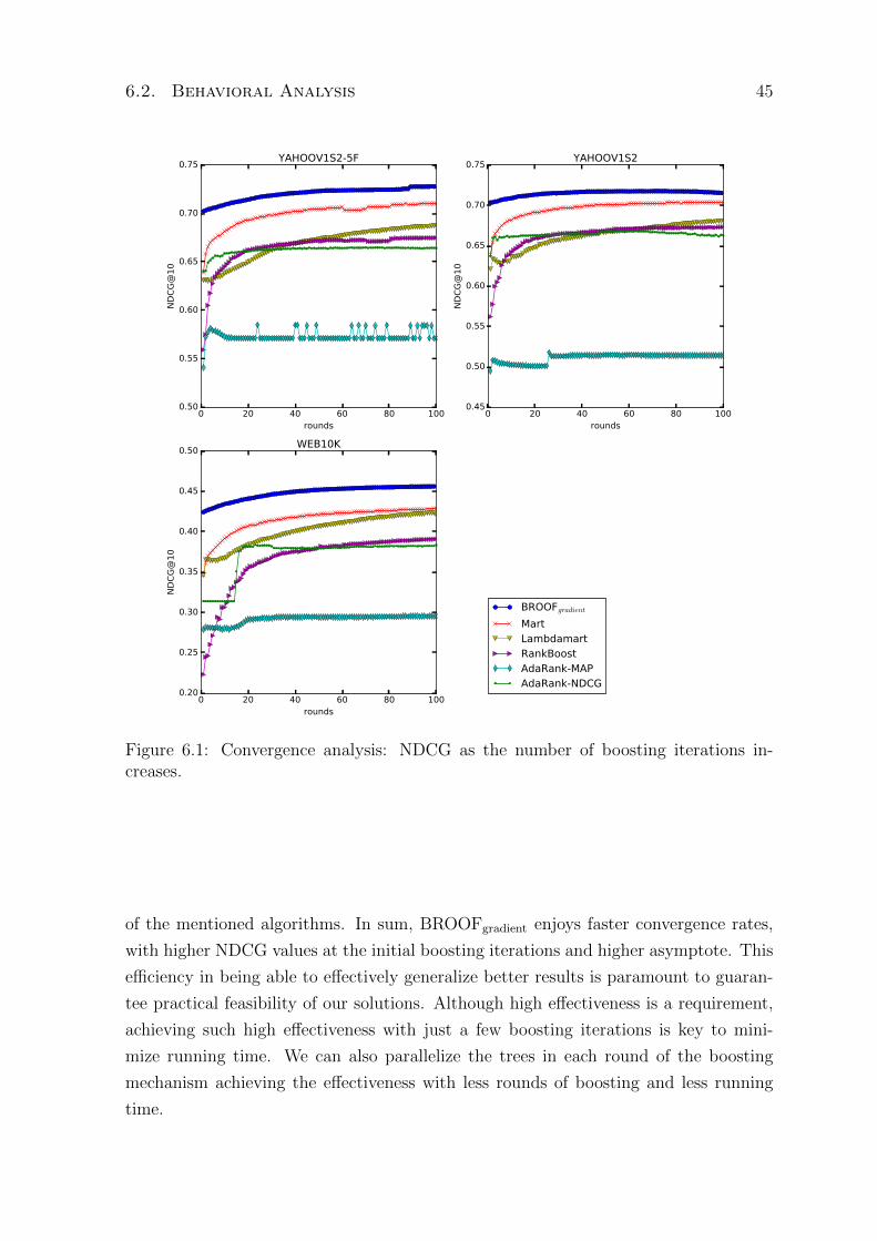
6.2. Behavioral Analysis 45
0 20 40 60 80 100rounds
0.50
0.55
0.60
0.65
0.70
0.75N
DC
G@
10
YAHOOV1S2-5F
0 20 40 60 80 100rounds
0.45
0.50
0.55
0.60
0.65
0.70
0.75
ND
CG
@1
0
YAHOOV1S2
0 20 40 60 80 100rounds
0.20
0.25
0.30
0.35
0.40
0.45
0.50
ND
CG
@1
0
WEB10K
BROOFgradient
MartLambdamartRankBoostAdaRank-MAPAdaRank-NDCG
Figure 6.1: Convergence analysis: NDCG as the number of boosting iterations in-creases.
of the mentioned algorithms. In sum, BROOFgradient enjoys faster convergence rates,
with higher NDCG values at the initial boosting iterations and higher asymptote. This
efficiency in being able to effectively generalize better results is paramount to guaran-
tee practical feasibility of our solutions. Although high effectiveness is a requirement,
achieving such high effectiveness with just a few boosting iterations is key to mini-
mize running time. We can also parallelize the trees in each round of the boosting
mechanism achieving the effectiveness with less rounds of boosting and less running
time.
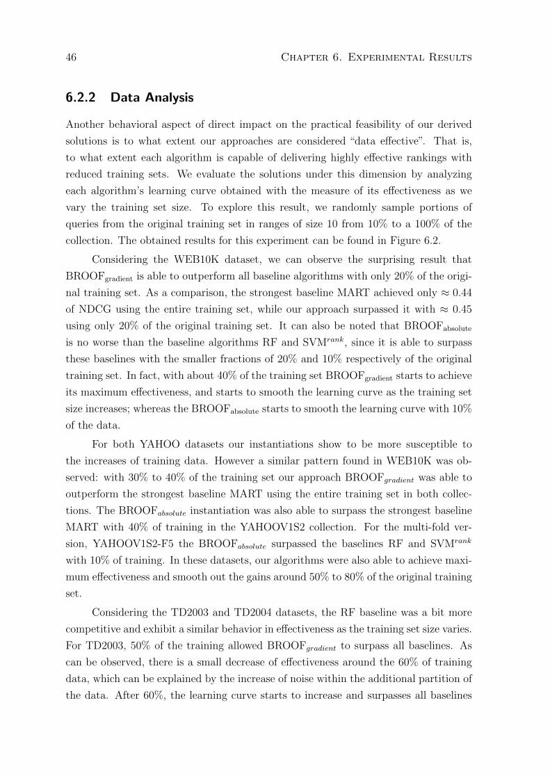
46 Chapter 6. Experimental Results
6.2.2 Data Analysis
Another behavioral aspect of direct impact on the practical feasibility of our derived
solutions is to what extent our approaches are considered “data effective”. That is,
to what extent each algorithm is capable of delivering highly effective rankings with
reduced training sets. We evaluate the solutions under this dimension by analyzing
each algorithm’s learning curve obtained with the measure of its effectiveness as we
vary the training set size. To explore this result, we randomly sample portions of
queries from the original training set in ranges of size 10 from 10% to a 100% of the
collection. The obtained results for this experiment can be found in Figure 6.2.
Considering the WEB10K dataset, we can observe the surprising result that
BROOFgradient is able to outperform all baseline algorithms with only 20% of the origi-
nal training set. As a comparison, the strongest baseline MART achieved only ≈ 0.44
of NDCG using the entire training set, while our approach surpassed it with ≈ 0.45
using only 20% of the original training set. It can also be noted that BROOFabsolute
is no worse than the baseline algorithms RF and SVMrank, since it is able to surpass
these baselines with the smaller fractions of 20% and 10% respectively of the original
training set. In fact, with about 40% of the training set BROOFgradient starts to achieve
its maximum effectiveness, and starts to smooth the learning curve as the training set
size increases; whereas the BROOFabsolute starts to smooth the learning curve with 10%
of the data.
For both YAHOO datasets our instantiations show to be more susceptible to
the increases of training data. However a similar pattern found in WEB10K was ob-
served: with 30% to 40% of the training set our approach BROOFgradient was able to
outperform the strongest baseline MART using the entire training set in both collec-
tions. The BROOFabsolute instantiation was also able to surpass the strongest baseline
MART with 40% of training in the YAHOOV1S2 collection. For the multi-fold ver-
sion, YAHOOV1S2-F5 the BROOFabsolute surpassed the baselines RF and SVMrank
with 10% of training. In these datasets, our algorithms were also able to achieve maxi-
mum effectiveness and smooth out the gains around 50% to 80% of the original training
set.
Considering the TD2003 and TD2004 datasets, the RF baseline was a bit more
competitive and exhibit a similar behavior in effectiveness as the training set size varies.
For TD2003, 50% of the training allowed BROOFgradient to surpass all baselines. As
can be observed, there is a small decrease of effectiveness around the 60% of training
data, which can be explained by the increase of noise within the additional partition of
the data. After 60%, the learning curve starts to increase and surpasses all baselines
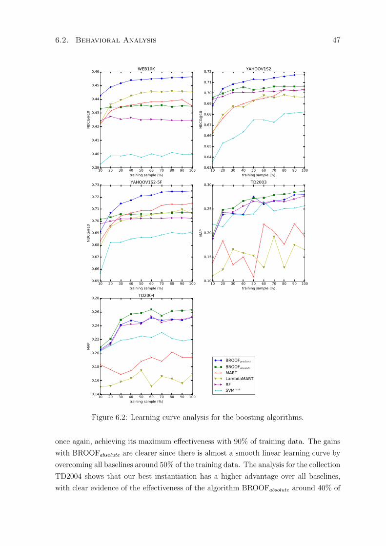
6.2. Behavioral Analysis 47
10 20 30 40 50 60 70 80 90 100training sample (%)
0.39
0.40
0.41
0.42
0.43
0.44
0.45
0.46
ND
CG
@10
WEB10K
10 20 30 40 50 60 70 80 90 100training sample (%)
0.63
0.64
0.65
0.66
0.67
0.68
0.69
0.70
0.71
0.72
ND
CG
@10
YAHOOV1S2
10 20 30 40 50 60 70 80 90 100training sample (%)
0.65
0.66
0.67
0.68
0.69
0.70
0.71
0.72
0.73
ND
CG
@10
YAHOOV1S2-5F
10 20 30 40 50 60 70 80 90 100training sample (%)
0.10
0.15
0.20
0.25
0.30
MA
P
TD2003
10 20 30 40 50 60 70 80 90 100training sample (%)
0.14
0.16
0.18
0.20
0.22
0.24
0.26
0.28
MA
P
TD2004
BROOFgradientBROOFabsoluteMARTLambdaMARTRFSVMrank
Figure 6.2: Learning curve analysis for the boosting algorithms.
once again, achieving its maximum effectiveness with 90% of training data. The gains
with BROOFabsolute are clearer since there is almost a smooth linear learning curve by
overcoming all baselines around 50% of the training data. The analysis for the collection
TD2004 shows that our best instantiation has a higher advantage over all baselines,
with clear evidence of the effectiveness of the algorithm BROOFabsolute around 40% of
48 Chapter 6. Experimental Results
training against the entire training data for the strongest baseline RF. BROOFgradient
is also quite competitive since it is tied with the RF surpassing all remaining baselines.
These findings have also a direct influence on the practical feasibility of our solu-
tions. First, smaller training set translates to smaller running times. Second, obtaining
labeled data is critical but also costly, thus it is clear that being able to produce highly
effective models from smaller training set is an important characteristic of a successful
approach.
6.2.3 Validation Analysis
As mentioned in the description of the extension points for Algorithm 1, the validation
set function in our boosting approaches enables to determine which training data sam-
ples will be considered during the weight update step. As described in the extension
points, there are basically two ways of selectively update the samples distribution. The
default procedure in most of the boosting strategies is to use the entire set of training
samples. As we argued during the description of the extension points, this update
strategy is in theory too optimistic, because it uses samples that were already used
during the construction of the model, which might cause overfitting as the number of
iterations increases. A better solution would be to use a cross-validation procedure of
the training samples, and apply these samples to assess the performance of the model
at each round of the boosting mechanism. Since we are using a RF model as the inner
procedure of the boosting, we recommend the use of out-of-bag samples as an option
of the validation procedure of our instances. Therefore, it is worth to assess the effect
of the use of the validation procedure with both training and out-of-bag samples to be
updated at each round of boosting. The results of this experiment are shown in Figure
6.3 for the three largest collections depicting the effectiveness of the BROOFgradient
approach (the best algorithm in these collections) as the number of rounds of boosting
increases. In these charts, the circled blue points represent the configuration for the
training samples while the red cross points represent the out-of-bag samples.
As we can observe in the charts for the depicted experiment, the results for the
YAHOOV1S2 collection show no difference in effectiveness in both validation techniques
until the round ≈ 50 of the boosting procedure. After this round, the learning curve
shows to overfit for the configuration of the validation procedure set to the out-of-
bag samples, while the configuration set to the training samples seems to grow as the
number of rounds increase. This is an interesting finding when contrasted with the
results for the folded version of the same collection using the 5-fold cross validation
procedure. As we can observe, the chart for the YAHOOV1S2-5F shows that there is
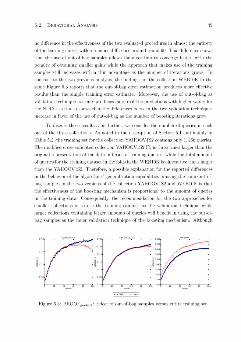
6.2. Behavioral Analysis 49
no difference in the effectiveness of the two evaluated procedures in almost the entirety
of the learning curve, with a tenuous difference around round 90. This difference shows
that the use of out-of-bag samples allows the algorithm to converge faster, with the
penalty of obtaining smaller gains while the approach that makes use of the training
samples still increases with a thin advantage as the number of iterations grows. In
contrast to the two previous analysis, the findings for the collection WEB10K in the
same Figure 6.3 reports that the out-of-bag error estimation produces more effective
results than the simple training error estimate. Moreover, the use of out-of-bag as
validation technique not only produces more realistic predictions with higher values for
the NDCG as it also shows that the differences between the two validation techniques
increase in favor of the use of out-of-bag as the number of boosting iterations grow.
To discuss these results a bit further, we consider the number of queries in each
one of the three collections. As noted in the description of Section 5.1 and mainly in
Table 5.2, the training set for the collection YAHOOV1S2 contains only 1, 266 queries.
The modified cross-validated collection YAHOOV1S2-F5 is three times larger than the
original representation of the data in terms of training queries, while the total amount
of queries for the training dataset in the folds in the WEB10K is almost five times larger
than the YAHOOV1S2. Therefore, a possible explanation for the reported differences
in the behavior of the algorithms’ generalization capabilities in using the train/out-of-
bag samples in the two versions of the collection YAHOOV1S2 and WEB10K is that
the effectiveness of the boosting mechanism is proportional to the amount of queries
in the training data. Consequently, the recommendation for the two approaches for
smaller collections is to use the training samples as the validation technique while
larger collections containing larger amounts of queries will benefit in using the out-of-
bag samples as the inner validation technique of the boosting mechanism. Although
0 20 40 60 80 100rounds
0.705
0.710
0.715
0.720
ND
CG
@10
YAHOOV1S2
0 20 40 60 80 100rounds
0.700
0.705
0.710
0.715
0.720
0.725
0.730
ND
CG
@10
YAHOOV1S2-5F
0 20 40 60 80 100rounds
0.420
0.425
0.430
0.435
0.440
0.445
0.450
0.455
0.460
0.465
ND
CG
@10
WEB10K
train oob
Figure 6.3: BROOFgradient: Effect of out-of-bag samples versus entire training set.

50 Chapter 6. Experimental Results
this is not a general rule of thumb, it is a good start point to take into consideration
before building boosted ensemble models based in bagged decision trees such as RF.
This highlights the importance of exploiting the validation set function as de-
scribed in Algorithm 1 in our proposed framework instantiations. As a final remark, as
it can be observed in the results of Figure 6.3, the variants that use the training error
rate are also able to outperform the baselines. This is also an important aspect that
highlights the quality of the proposed framework.
6.3 Quantitative Analysis
In this section, we report the full factorial experimental design with replication used to
explain the importance of the factors of the proposed framework and how they interact
among themselves. The importance of each factor and its interaction is given by the
computation of the allocation of variation and the statistical analysis of variance as
described by [Jain, 1991].
6.3.1 Full Factorial Design
As discussed in the previous analysis of this chapter, two factors are the most impor-
tant ones in the derived instantiations of our framework. They are: (i) the validation
set function and (ii) the loss functions used to minimize the residues at each boosting
iteration. The analysis for each individual L2R collection was managed considering a
full factorial design with the two aforementioned factors at two and four levels respec-
tively. The first factor considers whether the inner validation technique makes use of
training or out-of-bag samples in the updating strategy of the samples weights’ distri-
bution while the second factor takes into consideration each one the loss functions that
generates the derived instances of the framework named BROOFabsolute, BROOFregion,
BROOFheight and BROOFgradient.
The sample representation of the factorial design is shown in Table 6.3 for the
collection WEB10K. The columns out-of-bag and training represent the two levels of
the factor validation set function while the column containing the conglomeration of
algorithms in the rows of the table represents the second discrete factor: loss functions.
In order to discriminate the interactions and influence of the factors isolating the ex-
perimental errors, each experiment was repeated under each configuration 10 times for
each one of the evaluated collections.
The model of the full two-factor design with repetition is given by: yijk = µ +
αj + βi + γij + eij and the explanation of the fragmented parts of the equation are:

6.3. Quantitative Analysis 51
Algorithm Exp. Number Out-of-Bag Training
BROOFabsolute
1 0.43498 0.433842 0.43506 0.433963 0.43498 0.43388...
......
10 0.43476 0.43498
BROOFmedian
1 0.43566 0.436342 0.43604 0.435843 0.43568 0.43626...
......
10 0.4355 0.43514
BROOFheight
1 0.4288 0.42812 0.42902 0.428423 0.42904 0.42858...
......
10 0.4288 0.4277
BROOFgradient
1 0.45614 0.456082 0.45614 0.455843 0.4564 0.45614...
......
10 0.45628 0.45576
Table 6.3: NDCG@10 for the 4 instantiations of the proposed framework applied uponthe WEB10K in order to represent the full factor factorial design.
yijk is the knth observation of the factor A (validation set) at level j and factor B
(loss function) at level i
µ is the mean response for the k repetitions
αj is the effect of factor A at level j
βi is the effect of factor B at level i
γij is the interaction for the factors A at level i and B at level j.
eijk is the experimental error
6.3.2 Computation of effects
To compute the factors’ effects, it is necessary to arrange the observations in a two-
dimensional matrix such as the one shown in Table 6.3 consisting of b rows and a
columns such that the (i, j)th entry yij corresponds to the response in the experiment in
which factorA is at level j and factorB is at level i, which produces yij = µ+αj+βi+γij.
After the arrangement of the collected data, it is necessary to average the k repetitions

52 Chapter 6. Experimental Results
under each cell configuration in a new matrix as shown in Table 6.4 for each collection
(the measure metric is MAP for binary collections and NDCG@10 for multi-relevance
judgment collections averaged over the 10 replications under each configuration), and
then compute the means and sums of the observation for the new rows and columns
of the newly created table. As we can observe in this new table, by averaging over all
means observations we obtain the overall mean or mean response µ. The difference of
the row mean at level j minus the overall mean is the βi effect for the factor B at level
j which leads to the equation βi = yi..−µ that computes the column effects. The same
procedure applied on columns of this new table produces the effects αj for the factor
A, leading to the equation αi = y.j. − µ to compute the row effects.
The interpretation of the effects in Table 6.4 is as follows: the overall mean µ
explains that an average algorithm, using both the training and training and out-of-
bag samples, would obtain the values 0.2779 for TD2003, 0.2531 for TD2004, 0.7102
for YAHOOV1S2, 0.7111 for YAHOOV1S2-F5 and 0.43875 for WEB10K, considering
MAP and NDCG@10. It is also possible to observe in the column effect that the use of
out-of-bag samples provides a better ranking model than using the training samples for
the collections TD2003, TD2004 and WEB10K. Regarding the row effect that shows
the representativeness of the loss functions when compared to the average algorithm,
it is possible to observe that BROOFgradient and BROOFabsolute are better predictors
in TD2003. The collection TD2004 shows that three of the derived instantiations are
better than an average algorithm. For the three largest collections, BROOFgradient is
the only instance that showed to have an increase in NDCG@10.
The interactions of the two factors shown in Table 6.5 are computed by subtract-
ing the µ+αj +βi from the cell mean yij. in Table 6.4. Each produced cell corresponds
to the interaction of the two evaluated factors and its related levels. In this table is
possible to summarize that BROOFgradient and BROOFabsolute are 0.0049 and 0.0082
bellow the average derivations of the framework, while BROOFmedian and BROOFheight
show an increase in the performance for collection TD2003. When observing the find-
ings for TD2004 we can observe the same behavior for the algorithms BROOFgradient,
BROOFabsolute and BROOFheight with the instantiation BROOFmedian above the ave-
rage instantiations of the framework. The findings for YAHOOV1S2 shows that 3 out
of 4 derived instantiations are able to surpass the average case, with BROOFheight
being the only one which does not achieve the average algorithm. The interactions
for YAHOOV1S2 show that BROOFgradient and BROOFmedian are the only derivations
capable of surpassing an average algorithm, while YAHOOV1S2-5F only the instanti-
ations BROOFmedian and BROOFheight have some advantage over the average derived
instantiations of the framework in both alternatives of the validation set function.
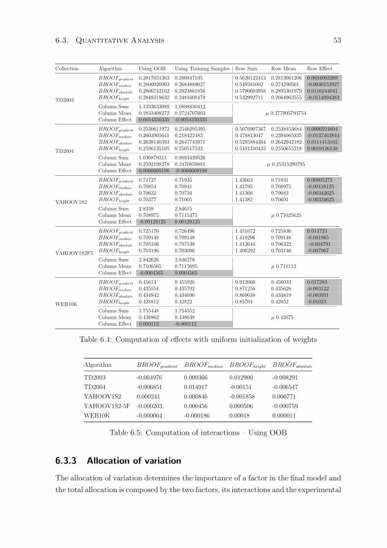
6.3. Quantitative Analysis 53
Collection Algorithm Using OOB Using Training Samples Row Sum Row Mean Row Effect
BROOFgradient 0.2817651363 0.280847105 0.5626122413 0.2813061206 0.0034003269BROOFmedian 0.2800920993 0.2684889027 0.548581002 0.274290501 -0.0036152927BROOFabsolute 0.2866742102 0.2923861856 0.5790603958 0.2895301979 0.0116244041BROOFheight 0.2848318632 0.2481608478 0.532992711 0.2664963555 -0.0114094383
Column Sum 1.1333633089 1.0898830412Column Mean 0.2833408272 0.2724707603
TD2003
Column Effect 0.0054350335 -0.0054350335µ 0.277905793754
BROOFgradient 0.2530611972 0.2546295395 0.5076907367 0.2538453684 0.0006924604BROOFmedian 0.2603905641 0.218422483 0.478813047 0.2394065235 -0.0137463844BROOFabsolute 0.2638140393 0.2647743971 0.5285884364 0.2642942182 0.0111413102BROOFheight 0.2596135105 0.250517533 0.5101310435 0.2550655218 0.0019126138
Column Sum 1.036879311 0.9883439526Column Mean 0.2592198278 0.2470859881
TD2004
Column Effect 0.0060669198 -0.0060669198µ 0.25315290795
BROOFgradient 0.71727 0.71935 1.43662 0.71831 0.00805375BROOFmedian 0.70854 0.70941 1.41795 0.708975 -0.00128125BROOFabsolute 0.70632 0.70734 1.41366 0.70683 -0.00342625BROOFheight 0.70377 0.71005 1.41382 0.70691 -0.00334625
Column Sum 2.8359 2.84615Column Mean 0.708975 0.7115375 µ 0.71025625
YAHOOV1S2
Column Effect -0.00128125 0.00128125
BROOFgradient 0.725176 0.726496 1.451672 0.725836 0.014723BROOFmedian 0.709148 0.709148 1.418296 0.709148 -0.001965BROOFabsolute 0.705106 0.707538 1.412644 0.706322 -0.004791BROOFheight 0.703196 0.703096 1.406292 0.703146 -0.007967
Column Sum 2.842626 2.846278Column Mean 0.7106565 0.7115695 µ 0.711113
YAHOOV1S2F5
Column Effect -0.0004565 0.0004565
BROOFgradient 0.45614 0.455926 0.912066 0.456033 0.017283BROOFmedian 0.435554 0.435702 0.871256 0.435628 -0.003122BROOFabsolute 0.434942 0.434696 0.869638 0.434819 -0.003931BROOFheight 0.428812 0.42822 0.85704 0.42852 -0.01023
Column Sum 1.755448 1.754552Column Mean 0.438862 0.438638 µ 0.43875
WEB10K
Column Effect 0.000112 -0.000112
Table 6.4: Computation of effects with uniform initialization of weights
Algorithm BROOFgradient BROOFmedian BROOFheight BROOFabsolute
TD2003 -0.004976 0.000366 0.012900 -0.008291
TD2004 -0.006851 0.014917 -0.00151 -0.006547
YAHOOV1S2 0.000241 0.000846 -0.001858 0.000771
YAHOOV1S2-5F -0.000203 0.000456 0.000506 -0.000759
WEB10K -0.000004 -0.000186 0.00018 0.000011
Table 6.5: Computation of interactions – Using OOB
6.3.3 Allocation of variation
The allocation of variation determines the importance of a factor in the final model and
the total allocation is composed by the two factors, its interactions and the experimental
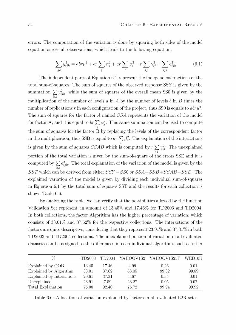
54 Chapter 6. Experimental Results
errors. The computation of the variation is done by squaring both sides of the model
equation across all observations, which leads to the following equation:
∑ijk
y2ijk = abrµ2 + br∑j
α2j + ar
∑i
β2i + r
∑ij
γ2ij +∑ijk
e2ijk (6.1)
The independent parts of Equation 6.1 represent the independent fractions of the
total sum-of-squares. The sum of squares of the observed response SSY is given by the
summation∑ijk
y2ijk, while the sum of squares of the overall mean SS0 is given by the
multiplication of the number of levels a in A by the number of levels b in B times the
number of replications r in each configuration of the project, thus SS0 is equals to abrµ2.
The sum of squares for the factor A named SSA represents the variation of the model
for factor A, and it is equal to br∑j
α2j . This same summation can be used to compute
the sum of squares for the factor B by replacing the levels of the correspondent factor
in the multiplication, thus SSB is equal to ar∑i
β2i . The explanation of the interactions
is given by the sum of squares SSAB which is computed by r∑ij
γ2ij. The unexplained
portion of the total variation is given by the sum-of-square of the errors SSE and it is
computed by∑ijk
e2ijk. The total explanation of the variation of the model is given by the
SST which can be derived from either SSY −SS0 or SSA+SSB+SSAB+SSE. The
explained variation of the model is given by dividing each individual sum-of-squares
in Equation 6.1 by the total sum of squares SST and the results for each collection is
shown Table 6.6.
By analyzing the table, we can verify that the possibilities allowed by the function
Validation Set represent an amount of 13.45% and 17.46% for TD2003 and TD2004.
In both collections, the factor Algorithm has the higher percentage of variation, which
consists of 33.01% and 37.62% for the respective collections. The interactions of the
factors are quite descriptive, considering that they represent 23.91% and 37.31% in both
TD2003 and TD2004 collections. The unexplained portion of variation in all evaluated
datasets can be assigned to the differences in each individual algorithm, such as other
% TD2003 TD2004 YAHOOV1S2 YAHOOV1S25F WEB10K
Explained by OOB 13.45 17.46 4.99 0.26 0.01Explained by Algorithm 33.01 37.62 68.05 99.32 99.89Explained by Interactions 29.61 37.31 3.67 0.35 0.01Unexplained 23.91 7.59 23.27 0.05 0.07Total Explanation 76.08 92.40 76.72 99.94 99.92
Table 6.6: Allocation of variation explained by factors in all evaluated L2R sets.
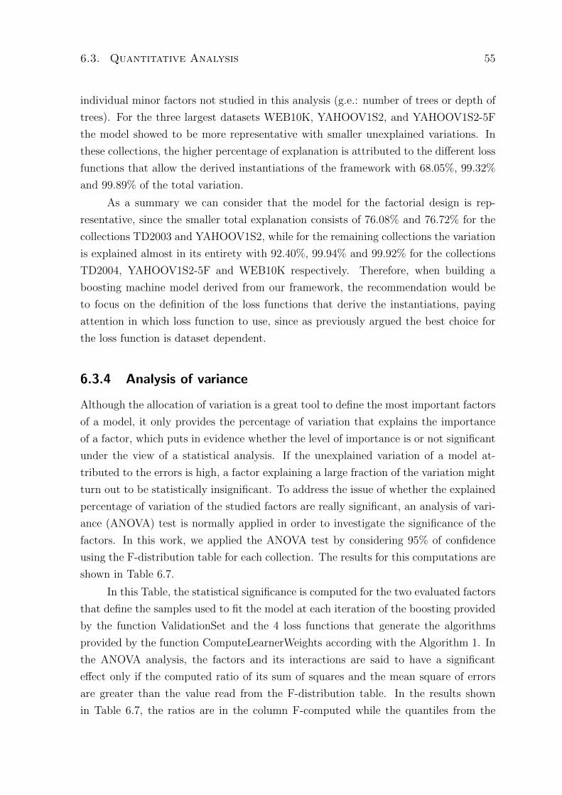
6.3. Quantitative Analysis 55
individual minor factors not studied in this analysis (g.e.: number of trees or depth of
trees). For the three largest datasets WEB10K, YAHOOV1S2, and YAHOOV1S2-5F
the model showed to be more representative with smaller unexplained variations. In
these collections, the higher percentage of explanation is attributed to the different loss
functions that allow the derived instantiations of the framework with 68.05%, 99.32%
and 99.89% of the total variation.
As a summary we can consider that the model for the factorial design is rep-
resentative, since the smaller total explanation consists of 76.08% and 76.72% for the
collections TD2003 and YAHOOV1S2, while for the remaining collections the variation
is explained almost in its entirety with 92.40%, 99.94% and 99.92% for the collections
TD2004, YAHOOV1S2-5F and WEB10K respectively. Therefore, when building a
boosting machine model derived from our framework, the recommendation would be
to focus on the definition of the loss functions that derive the instantiations, paying
attention in which loss function to use, since as previously argued the best choice for
the loss function is dataset dependent.
6.3.4 Analysis of variance
Although the allocation of variation is a great tool to define the most important factors
of a model, it only provides the percentage of variation that explains the importance
of a factor, which puts in evidence whether the level of importance is or not significant
under the view of a statistical analysis. If the unexplained variation of a model at-
tributed to the errors is high, a factor explaining a large fraction of the variation might
turn out to be statistically insignificant. To address the issue of whether the explained
percentage of variation of the studied factors are really significant, an analysis of vari-
ance (ANOVA) test is normally applied in order to investigate the significance of the
factors. In this work, we applied the ANOVA test by considering 95% of confidence
using the F-distribution table for each collection. The results for this computations are
shown in Table 6.7.
In this Table, the statistical significance is computed for the two evaluated factors
that define the samples used to fit the model at each iteration of the boosting provided
by the function ValidationSet and the 4 loss functions that generate the algorithms
provided by the function ComputeLearnerWeights according with the Algorithm 1. In
the ANOVA analysis, the factors and its interactions are said to have a significant
effect only if the computed ratio of its sum of squares and the mean square of errors
are greater than the value read from the F-distribution table. In the results shown
in Table 6.7, the ratios are in the column F-computed while the quantiles from the
56 Chapter 6. Experimental Results
Collection Component Sum of Squares % of Variation Deg. of Fr. Mean Square F-computed F-Table
TD2003
y 6.196094 80y . . . 6.178530 1y − y . . . 0.017563 100.0 79Use Of OOB 0.002363 13.454867 1 0.002363 0.031254 3.973896Algorithm 0.005798 33.015286 3 0.001932 0.025563 2.731807Interactions 0.005201 29.613235 3 0.001733 0.022929 2.731807Errors 0.004200 23.916609 72 0.075611
se = 0.027497
TD2004
y 5.143774 80y . . . 5.126911 1y − y . . . 0.016862 100.0 79Use Of OOB 0.002944 17.461974 1 0.002944 0.127688 3.973896Algorithm 0.006344 37.624468 3 0.002114 0.091708 2.731807Interactions 0.006292 37.316113 3 0.002097 0.090956 2.731807Errors 0.001281 7.597443 72 0.023060
se = 0.015185
YAHOOV1S2
y 40.359743 80y . . . 40.357115 1y-y . . . 0.002628 100 79Use Of OOB 0.000131 4.996548 1 0.000131 0.011926 3.973896Algorithm 0.001788 68.058024 3 0.000596 0.054150 2.731807Interactions 9.6482375e-05 3.670796 3 3.21607916667e-05 0.002920 2.731807Errors 0.000611 23.274630 72 0.011011
se = 0.010493
YAHOOV1S2F5
y 40.460718 80y . . . 40.454535 1y-y . . . 0.006182 100 79Use Of OOB 1.667138e-05 0.269644 1 1.667138e-05 0.281338 3.973896Algorithm 0.006141 99.326717 3 0.002047 34.544717 2.731807Interactions 2.166374e-05 0.350391 3 7.22124666667e-06 0.121862 2.731807Errors 3.29207998409e-06 0.053246 72 5.92574397136e-05
se = 0.000769
WEB10K
y 15.408704 80y . . . 15.400125 1y-y . . . 0.008579 100 79Use Of OOB 1.00352e-06 0.011696 1 1.00352e-06 0.008508 3.973896Algorithm 0.008571 99.896287 3 0.002857 24.224673 2.731807Interactions 1.34284e-06 0.015650 3 4.47613333333e-07 0.003795 2.731807Errors 6.55216000306e-06 0.076365 72 0.000117
se = 0.001085
Table 6.7: ANOVA using 95% of confidence level
F-distribution are shown in the column F-Table.
By analyzing the ratio of all three components of the allocation of variation
shown in these two columns for the collection TD2003, we can conclude that there is
no statistical evidence that one factor alone or even its interactions provides significant
difference amongst the obtained results of the derived instantiations and that the ob-
served difference in the obtained metric measures are mostly due to the unexplained
variation, which is congruent to the obtained results shown in the allocation of variation
analysis for the collection TD2003. The same behavior is observed for the collections
TD2004 and YAHOOV1S2 in all three evaluated components allowing us to conclude
that the obtained results are merely due to the experimental errors and not to any

6.3. Quantitative Analysis 57
significant difference between the loss functions or the different out-of-bag or training
samples used during the boosting iterations. For both collections, YAHOOV1S2-F5
and WEB10K are possible to observe a different behavior from the three previously
one, which allow us to conclude that the choice of the loss functions is congruent to
the higher percentage of variation of over 99% in both collections. In summary, we
can conclude that regarding the instantiations of the framework the most significant
factor is the use of the right loss function since it is more prone to give advantages
with statistical evidence using an ANOVA test than using the training or out-of-bag
samples.

Chapter 7
Conclusions and Future Work
In this chapter, we summarize the research contributions of this master degree thesis
and point out some lines of research for further investigation.
7.1 The Framework
In this work, we proposed an extensible framework for L2R, called Generalized BROOF-
L2R, which smoothly combines two successful strategies for Learning to Rank, namely,
Random Forests and Boosting. Such combination, that uses Random Forests models
as weak learners for the boosting algorithm, relies on a set of functions that must be
set in order to derive instantiations of the framework. The main characteristics of the
framework are: (i) to make use of the training or out-of-bag samples produced by
bagging procedures such as Random Forests to determine the influence of each weak
learner in the final additive model and (ii) to update the sample distribution weights by
means of a more reliable error rate estimate through the applied loss functions. In fact,
the framework is general enough to provide a rather heterogeneous set of instantiations
that, according to our empirical evaluation, are able to achieve competitive results
compared to state-of-the-art algorithms for L2R.
Amongst the set of possible combinations, we only evaluated a total of eight possi-
ble instantiations by setting the validation set to training an out-of-bag with 4 distinct
loss functions. Regarding the loss functions used in the derived instantiations, three of
them relate to boosting by re-weighting. They sequentially minimize the residues at
each iteration by building Random Forests as weak learners that are specialists in hard
to predict regions by means of perturbation of the input space in the samples weights’
distributions. The fourth loss function is based on gradient descent optimization, which
59

60 Chapter 7. Conclusions and Future Work
sequentially minimizes the residues by updating the original underlying ground truth
for the training samples, thus making boosted gradient random forests models.
Despite the fact that all derived instances of the framework provide very com-
petitive results when compared to the evaluated baselines, BROOFgradient seems to
be consistently the top performer in the larger collections, followed by the remai-
ning derivations that are also superior to most baselines. For the smaller collections,
BROOFabsolute seems to be the best performer, with all other derivations being very
competitive, surpassing or tying with most baselines. According to our experimental
analysis, all our instantiations are prone to achieve superior results when contrasted to
the baseline algorithms under a scenario of a constrained amount of training samples
with faster convergence rate. Another observed trend when contrasting the use of the
validations set techniques is that using training samples seems to be a better choice for
smaller collections, while the use of out-of-bag samples increases the algorithms gener-
alization capabilities as the size of the data increases. We also investigated the effects
and the allocation of variation for the two main factors of the proposed framework,
which lead led us to conclude that amongst the eight derived instantiations by varying
the 4 loss functions and the two inner validation techniques, the most representative
factor is the set of the loss function, explaining the largest evidence in the allocation
of variation and in the ANOVA test.
7.2 Future Work
We believe that there is a lot of ground to cover regarding our ML approaches. For
instance, based on our initial analysis, besides the envisioned loss functions, there are
other important factors that can be generalized in our previous solution, including:
(i) the initialization strategy to define the importance of samples in each query on
the training set; (ii) how to update the samples. Moreover, although we quantify the
use of the four loss functions and the use of samples in the inner validation technique
of the boosting procedure in a factorial design, we still need to really quantify the
impact of the remaining components of our solution in the final results in order to
analyze the most promising ways of improving instantiations of the framework. The
allocation of variation that was possible to identify with statistical significance were
only observed in WEB10K and YAHOOV1S2-F5, with unexplained variation for the
remaining collections, which can be attributed to the remaining not studied factors.
In fact, based on the aspects we can vary in our procedures we have envisioned a
minimum of 16 possible instantiations of our general L2R framework by combining

7.2. Future Work 61
the possibilities shown in Algorithm 1, from which we tested only 8, which are already
superior to the state-of-the-art. This demonstrates the potential of continuing to pursue
this line of research. One possibility, for instance, is to modify the initial distribution
to a more uniform model, such as the Dirichlet randomization factor, and assess the
performance of the variations over the training set (original boosting procedures) and
out-of-bag procedures. It is also possible to modify the validation procedure, such that
the inner validation technique of the boosting procedure induces leave-one-out queries
in the training, instead of relying only on the out-of-bag or training samples to lead
the weak learners to the hard regions of the input space.
Other possible extension regards our fourth loss function. This relates to its
resemblance to the Mart algorithm (one of the most effective ones in L2R). We conjec-
ture that, by considering that (i) Mart is an additive tree procedure that minimizes the
least-square regression loss using gradient descent and (ii) our approach is an additive
tree procedure based on an ensemble of averaged trees generated by the RF model,
we believe that we can use the same technique used by LambdaMart to enhance our
results by specifying appropriate gradients generated by the LambdaRank function
in each iteration of our weak-learners. Hitherto we were able to verify that Lamb-
daMart was able to surpass its base model Mart in some of the datasets by using the
multi-relevance judgment ranking metric NDCG, which if correctly applied upon our
base weak-learner will allow us to instantiate a new listwise approach using the same
properties of LambdaMart, but in our case with a larger potential.
Another hard to tackle issue regarding our boosting procedures refers to the
number of iterations to stop the boosting. In all our approaches we stop the boosting
iterations by setting a number of rounds that the algorithm must have. However, if
the chosen number is too large, a heuristic is applied that considers at each iteration
if the current model has an error higher than 1/2, and if so, the training is stopped
and no further weak learner is built to compose the ensemble. Although this approach
yields satisfying (statistically significant) results, we verified that it is far from perfect
and that by choosing a better strategy to stop the number of iterations would allow us
to leverage the performance of our rankers even further.
7.2.1 A few Guidelines for Future Investigation
To summarize, we intend to answer the following research questions in future work,
that we were not able to be investigate so far:
1. Is it worth to extend our current approach to a listwise one by exploring dif-
ferent loss functions in the learning phase? Before our current approach (a

62 Chapter 7. Conclusions and Future Work
pointwise one), the state-of-the-art in several datasets was a listwise approach
– LambdaMART. We are confident that we can extend BROOF-L2R in a list-
wise manner by exploiting the LambdaRank gradients used by LambdaMart. In
this algorithm, there is a large gap when we vary the underlying metric from
ERR to NDCG in different datasets. We propose to investigate these differences
in our framework and arrive in a feasible solution that does not require too much
parameterization on the training phase.
2. What is the best way to choose the stopping criteria in a boosting procedure? We
will investigate the possibility of assessing the best strategy to stop the boosting
iteration of our current approaches. One possibility is to use the correlation of
the number of rounds.
3. Is it worth to identify the statistical query dependencies based on a “leave-one-
out” strategy? We observed that by validating the training phase using leave-
one-out of the queries increases the performance of our approaches. We are
investigating the possibility of using this procedure as the underlying mechanism
to induce the weak learners into the hard to predict regions of the input space.
4. What are the main factors and their interactions in our current approaches?
We have considered only eight instantiations of our framework, and by simply
modifying some key concepts in each of them we are able to extend it to a whole
new family of algorithms.
5. What are the theoretical properties of our solutions? We have not delved deeper
into such questions in order to understand why our solutions work so well. For in-
stance, are we achieving a better trade-off between the bias and the variance of the
learned models with our solution? We intend to perform such investigations and
investigate how we can improve our framework with the use of regularization tech-
niques such as the ones proposed by [Hastie et al., 2015] and [Saha et al., 2013].

Bibliography
[Amaratunga et al., 2008] Amaratunga, D., Cabrera, J., and Lee, Y.-S. (2008). En-
riched random forests. Bioinformatics, 24(18):2010–2014.
[Antonio Criminisi, 2009] Antonio Criminisi, Jamie Shotton, S. B. (2009). Decision
forests with long-range spatial context for organ localization in ct volumes. In
MICCAI workshop on Probabilistic Models for Medical Image Analysis (MICCAI-
PMMIA).
[Baeza-Yates and Ribeiro-Neto, 1999] Baeza-Yates, R. A. and Ribeiro-Neto, B. (1999).
Modern Information Retrieval. Addison-Wesley Longman Publishing Co., Inc.,
Boston, MA, USA.
[Bernard et al., 2012] Bernard, S., Adam, S., and Heutte, L. (2012). Dynamic random
forests. Pattern Recognition Letters, 33(12):1580 – 1586.
[Breiman, 1996a] Breiman, L. (1996a). Bagging predictors. Machine Learning,
24(2):123–140.
[Breiman, 1996b] Breiman, L. (1996b). Out-of-bag estimation.
[Breiman, 2001] Breiman, L. (2001). Random forests. Machine Learning, 45(1):5–32.
[Breiman et al., 1984] Breiman, L., Friedman, J., Stone, C., and Olshen, R. (1984).
Classification and Regression Trees. The Wadsworth and Brooks-Cole statistics-
probability series. Taylor & Francis.
[Broder, 2002] Broder, A. (2002). A taxonomy of web search. SIGIR Forum, 36(2):3–
10.
[Burges, 2010] Burges, C. J. (2010). From ranknet to lambdarank to lambdamart: An
overview. Technical report.
63
64 BIBLIOGRAPHY
[Busa-Fekete et al., 2013] Busa-Fekete, R., Kegl, B., Eltet o, T., and Szarvas, G.
(2013). Tune and mix: learning to rank using ensembles of calibrated multi-class
classifiers. Machine Learning, 93(2-3):261–292.
[Canuto et al., 2013] Canuto, S. D., Belem, F. M., Almeida, J. M., and Goncalves,
M. A. (2013). A comparative study of learning-to-rank techniques for tag recom-
mendation. JIDM, 4(3):453–468.
[Chen and Ishwaran, 2012] Chen, X. and Ishwaran, H. (2012). Random forests for
genomic data analysis. Genomics, 99(6):323 – 329.
[de Sa et al., 2016] de Sa, C. C., Goncalves, M. A., Sousa, D. X., and Salles, T. (2016).
Generalized broof-l2r: A general framework for learning to rank based on boosting
and random forests. In Proceedings of the 39th International ACM SIGIR Conference
on Research and Development in Information Retrieval, SIGIR ’16, pages 95–104,
New York, NY, USA. ACM.
[de Sa et al., 2015] de Sa, C. C. A., Goncalves, M. A., de Sousa, D. X., and Salles, T.
(2015). Aprendendo a Ranquear com Boosting e Florestas Aleatorias: Um Modelo
Hıbrido. In Plastino, A., de Amo, S., and Marinho, L. B., editors, Symposium on
Knowledge Discovery, Mining and Learning, volume 1, pages 42–49, Petropolis, RJ,
Brazil.
[Demsar, 2006] Demsar, J. (2006). Statistical comparisons of classifiers over multiple
data sets. J. Mach. Learn. Res., 7:1–30.
[Drucker, 1997] Drucker, H. (1997). Improving regressors using boosting techniques. In
Proceedings of the Fourteenth International Conference on Machine Learning, ICML
’97, pages 107–115, San Francisco, CA, USA. Morgan Kaufmann Publishers Inc.
[Fernandez-Delgado et al., 2014] Fernandez-Delgado, M., Cernadas, E., Barro, S., and
Amorim, D. (2014). Do we need hundreds of classifiers to solve real world classifica-
tion problems? J. Mach. Learn. Res., 15(1):3133–3181.
[Freund et al., 2003] Freund, Y., Iyer, R., Schapire, R. E., and Singer, Y. (2003). An
efficient boosting algorithm for combining preferences. The Journal of Machine
Learning Research, 4:933–969.
[Freund and Schapire, 1996] Freund, Y. and Schapire, R. E. (1996). Experiments with
a New Boosting Algorithm. In ICML, pages 148–156.

BIBLIOGRAPHY 65
[Friedman, 2000] Friedman, J. H. (2000). Greedy function approximation: A gradient
boosting machine. Annals of Statistics, 29:1189–1232.
[Gao and Yang, 2014] Gao, W. and Yang, P. (2014). Democracy is good for ranking:
Towards multi-view rank learning and adaptation in web search. In Proceedings of
the 7th ACM International Conference on Web Search and Data Mining, WSDM
’14, pages 63–72, New York, NY, USA. ACM.
[Geurts et al., 2006] Geurts, P., Ernst, D., and Wehenkel, L. (2006). Extremely ran-
domized trees. Machine Learning, 63(1):3–42.
[Geurts and Louppe, 2011] Geurts, P. and Louppe, G. (2011). Learning to rank with
extremely randomized trees. In Proceedings of the Yahoo! Learning to Rank Chal-
lenge, held at ICML 2010, Haifa, Israel, June 25, 2010, pages 49–61.
[Granka et al., 2004] Granka, L. A., Joachims, T., and Gay, G. (2004). Eye-tracking
analysis of user behavior in www search. In Proceedings of the 27th Annual In-
ternational ACM SIGIR Conference on Research and Development in Information
Retrieval, SIGIR ’04, pages 478–479, New York, NY, USA. ACM.
[Hancock et al., 1996] Hancock, T., Jiang, T., Li, M., and Tromp, J. (1996). Lower
bounds on learning decision lists and trees. Information and Computation, 126(2):114
– 122.
[Hastie et al., 2009] Hastie, T., Tibshirani, R., and Friedman, J. H. (2009). The Ele-
ments of Statistical Learning. Springer.
[Hastie et al., 2015] Hastie, T., Tibshirani, R., and Wainwright, M. (2015). Statisti-
cal Learning with Sparsity: The Lasso and Generalizations. Chapman & Hall/CRC
Monographs on Statistics & Applied Probability. Chapman and Hall/CRC, first edi-
tion.
[He et al., 2008] He, C., Wang, C., xin Zhong, Y., and Li, R.-F. (2008). A survey on
learning to rank. In Machine Learning and Cybernetics, 2008 International Confer-
ence on, volume 3, pages 1734–1739.
[Jain, 1991] Jain, R. (1991). The art of computer systems performance analysis - tech-
niques for experimental design, measurement, simulation, and modeling. Wiley pro-
fessional computing. Wiley.
[Jiang, 2011] Jiang, L. (2011). Learning random forests for ranking. Frontiers of Com-
puter Science in China, 5(1):79–86.

66 BIBLIOGRAPHY
[Jin et al., 2003] Jin, R., Liu, Y., Si, L., Carbonell, J., and Hauptmann, A. G. (2003).
A new boosting algorithm using input-dependent regularizer. In ICML.
[Joachims, 2006] Joachims, T. (2006). Training linear svms in linear time. In ACM
SIGKDD, pages 217–226.
[Kotsiantis, 2011] Kotsiantis, S. (2011). Combining bagging, boosting, rotation forest
and random subspace methods. Artificial Intelligence Review, 35(3):223–240.
[Kuncheva, 2014] Kuncheva, L. I. (2014). Combining Pattern Classifiers: Methods and
Algorithms. Number 4. John Wiley & Sons, Inc., New Jersey, 2 edition.
[Liu, 2009] Liu, T.-Y. (2009). Learning to rank for information retrieval. Found. Trends
Inf. Retr., 3(3):225–331.
[Liu, 2011] Liu, T.-Y. (2011). Learning to Rank for Information Retrieval. Springer.
[Lucchese et al., 2016a] Lucchese, C., Nardini, F. M., Orlando, S., Perego, R., Silvestri,
F., and Trani, S. (2016a). Post-learning optimization of tree ensembles for efficient
ranking. In Proceedings of the 39th International ACM SIGIR conference on Re-
search and Development in Information Retrieval, SIGIR 2016, Pisa, Italy, July
17-21, 2016, pages 949–952.
[Lucchese et al., 2015] Lucchese, C., Nardini, F. M., Orlando, S., Perego, R., Tonel-
lotto, N., and Venturini, R. (2015). Quickscorer: A fast algorithm to rank documents
with additive ensembles of regression trees. In Proceedings of the 38th International
ACM SIGIR Conference on Research and Development in Information Retrieval,
SIGIR ’15, pages 73–82, New York, NY, USA. ACM.
[Lucchese et al., 2016b] Lucchese, C., Nardini, F. M., Orlando, S., Perego, R., Tonel-
lotto, N., and Venturini, R. (2016b). Exploiting cpu simd extensions to speed-up
document scoring with tree ensembles. In Proceedings of the 39th International ACM
SIGIR Conference on Research and Development in Information Retrieval, SIGIR
’16, pages 833–836, New York, NY, USA. ACM.
[Maimon and Rokach, 2010] Maimon, O. and Rokach, L. (2010). Classification trees.
In Maimon, O. and Rokach, L., editors, Data Mining and Knowledge Discovery
Handbook, chapter 9, pages 149–174. Springer US.
[Manning et al., 2008] Manning, C. D., Raghavan, P., and Schutze, H. (2008). In-
troduction to Information Retrieval. Cambridge University Press, New York, NY,
USA.

BIBLIOGRAPHY 67
[Mason et al., 2000] Mason, L., Baxter, J., Bartlett, P., and Frean, M. (2000). Boosting
algorithms as gradient descent. In In Advances in Neural Information Processing
Systems, pages 512–518.
[Menze et al., 2011] Menze, B. H., Kelm, B. M., Splitthoff, D. N., Koethe, U., and
Hamprecht, F. A. (2011). On Oblique Random Forests, pages 453–469. Springer
Berlin Heidelberg, Berlin, Heidelberg.
[Mishina et al., 2014] Mishina, Y., Tsuchiya, M., and Fujiyoshi, H. (2014). Boosted
random forest. In VISAPP 2014 - Proceedings of the 9th International Conference
on Computer Vision Theory and Applications, Volume 2, Lisbon, Portugal, 5-8 Jan-
uary, 2014, pages 594–598.
[Mohan et al., 2011] Mohan, A., Chen, Z., and Weinberger, K. Q. (2011). Web-search
ranking with initialized gradient boosted regression trees. In Proceedings of the
Yahoo! Learning to Rank Challenge, held at ICML 2010, Haifa, Israel, June 25,
2010, pages 77–89.
[Niu et al., 2012] Niu, S., Guo, J., Lan, Y., and Cheng, X. (2012). Top-k learning to
rank: Labeling, ranking and evaluation. In Proceedings of the 35th International
ACM SIGIR Conference on Research and Development in Information Retrieval,
SIGIR ’12, pages 751–760, New York, NY, USA. ACM.
[Park, 2010] Park, L. a. F. (2010). Confidence Intervals for Information Retrieval Eval-
uation. Australiasian Document Computing Symposium.
[Pass et al., 2006] Pass, G., Chowdhury, A., and Torgeson, C. (2006). A picture of
search. In Proceedings of the 1st International Conference on Scalable Information
Systems, InfoScale ’06, New York, NY, USA. ACM.
[Pedregosa et al., 2011] Pedregosa, F., Varoquaux, G., Gramfort, A., Michel, V.,
Thirion, B., Grisel, O., Blondel, M., Prettenhofer, P., Weiss, R., Dubourg, V., Van-
derplas, J., Passos, A., Cournapeau, D., Brucher, M., Perrot, M., and Duchesnay,
E. (2011). Scikit-learn: Machine learning in Python. Journal of Machine Learning
Research, 12:2825–2830.
[Quinlan, 1986] Quinlan, J. R. (1986). Induction of decision trees. Mach. Learn.,
1(1):81–106.
[Quinlan, 1993] Quinlan, J. R. (1993). C4.5: Programs for Machine Learning. Morgan
Kaufmann Publishers Inc., San Francisco, CA, USA.

68 BIBLIOGRAPHY
[Quinlan, 1996] Quinlan, J. R. (1996). Bagging, boosting, and c4.5. In Proceedings of
the Thirteenth National Conference on Artificial Intelligence - Volume 1, AAAI’96,
pages 725–730. AAAI Press.
[Saha et al., 2013] Saha, B. N., Kunapuli, G., Ray, N., Maldjian, J. A., and Natarajan,
S. (2013). AR-Boost: Reducing Overfitting by a Robust Data-Driven Regularization
Strategy, pages 1–16. Springer Berlin Heidelberg, Berlin, Heidelberg.
[Salles et al., 2015] Salles, T., Goncalves, M., Rodrigues, V., and Rocha, L. (2015).
Broof: Exploiting out-of-bag errors, boosting and random forests for effective au-
tomated classification. In Proceedings of the 38th International ACM SIGIR Con-
ference on Research and Development in Information Retrieval, SIGIR ’15, pages
353–362, New York, NY, USA. ACM.
[Santos et al., 2015] Santos, R. L. T., Macdonald, C., and Ounis, I. (2015). Search
result diversification. Foundations and Trends in Information Retrieval, 9(1):1–90.
[Schapire, 1990] Schapire, R. E. (1990). The strength of weak learnability. Mach.
Learn., 5(2):197–227.
[Schapire, 1999] Schapire, R. E. (1999). A brief introduction to boosting. In Proceed-
ings of the 16th International Joint Conference on Artificial Intelligence - Volume 2,
IJCAI’99, pages 1401–1406, San Francisco, CA, USA. Morgan Kaufmann Publishers
Inc.
[Schapire and Freund, 2012] Schapire, R. E. and Freund, Y. (2012). Boosting: Foun-
dations and Algorithms. The MIT Press.
[Shrestha and Solomatine, 2006] Shrestha, D. L. and Solomatine, D. P. (2006). Ex-
periments with adaboost.rt, an improved boosting scheme for regression. Neural
Comput., 18(7):1678–1710.
[Silverstein et al., 1999] Silverstein, C., Marais, H., Henzinger, M., and Moricz, M.
(1999). Analysis of a very large web search engine query log. SIGIR Forum, 33(1):6–
12.
[Solomatine and Shrestha, 2004] Solomatine, D. and Shrestha, D. (2004). AdaBoost.
RT: a boosting algorithm for regression problems. IEEE International Joint Con-
ference on Neural Networks, 2:1163–1168.
[Song et al., 2007] Song, R., Luo, Z., Wen, J.-R., Yu, Y., and Hon, H.-W. (2007).
Identifying ambiguous queries in web search. In Proceedings of the 16th International

BIBLIOGRAPHY 69
Conference on World Wide Web, WWW ’07, pages 1169–1170, New York, NY, USA.
ACM.
[Tan et al., 2005] Tan, P.-N., Steinbach, M., and Kumar, V. (2005). Introduction
to Data Mining, (First Edition). Addison-Wesley Longman Publishing Co., Inc.,
Boston, MA, USA.
[Tax et al., 2015] Tax, N., Bockting, S., and Hiemstra, D. (2015). A cross-benchmark
comparison of 87 learning to rank. Information Processing & Management, 51(6):757
– 772.
[Treeratpituk and Giles, 2009] Treeratpituk, P. and Giles, C. L. (2009). Disambiguat-
ing authors in academic publications using random forests. In Proceedings of the 9th
ACM/IEEE-CS Joint Conference on Digital Libraries, JCDL ’09, pages 39–48, New
York, NY, USA. ACM.
[Xu and Li, 2007] Xu, J. and Li, H. (2007). Adarank: A boosting algorithm for in-
formation retrieval. In Proceedings of the 30th Annual International ACM SIGIR
Conference on Research and Development in Information Retrieval, SIGIR ’07, pages
391–398, New York, NY, USA. ACM.
[Xu et al., 2012] Xu, Z. E., Weinberger, K. Q., and Chapelle, O. (2012). The greedy
miser: Learning under test-time budgets. In ICML.
[Zhang and Xie, 2010] Zhang, Z. and Xie, X. (2010). Research on AdaBoost.M1 with
Random Forest. In International Conference on Computer Engineering and Tech-
nology.