Embed Size (px)
Citation preview

Universidade de Lisboa
Faculdade de Ciências
Departamento de Física
EVALUATION OF THE D-SPECT SYSTEM:
Region Centric Acquisition and Tracer Kinetics
Filipa Alexandra Pina Barrento da Costa
Dissertação
Mestrado Integrado em Engenharia Biomédica e Biofísica
2012

Universidade de Lisboa
Faculdade de Ciências
Departamento de Física
EVALUATION OF THE D-SPECT SYSTEM:
Region Centric Acquisition and Tracer Kinetics
Filipa Alexandra Pina Barrento da Costa
Dissertação de Mestrado Integrado Orientada pelo Professor Pedro Almeida e pelo
Professor Brian Hutton
Mestrado Integrado em Engenharia Biomédica e Biofísica
2012

i
ACKNOWLEDGEMENTS
I would like to acknowledge all the people that made this thesis possible.
First I would like to thank my supervisor Professor Brian Hutton for the critical insights and
enthusiastic support and guidance throughout the work and my supervisor in Portugal, Professor Pedro
Almeida for helping me to find this opportunity of making this thesis at UCL, and for being always
available. I also want to thank my co-supervisor Professor Kjell Erlandsson for being always available
to answer my questions, given me very useful suggestions, essential for the progression of my work.
The research group, specially Alexandre Bousse, Niccolo Fuin and Maria Holstensson, were
very important for me during the internship. They made me feel welcome to the Institute, gave me
important advices and provided a good environment during my stay. Stefano Pedemonte also helped me
during my stay at the Institute. I also want to show my gratitude to Elizabeth Howell that kindly helped
me to understand the D-SPECT simulator and Benjamin Thomas, Ian Cullum and Shane for setting my
computer when it had some problems. I also acknowledge Rayjanah Allie for showing great interest in
my work and for the fascinating conversations, helping me understanding the clinical point of view of
my project.
I also want to thank my parents, Filomena e João, for the love and support, stimulating me to
keep motivated and doing the best I could. Thanks to my boyfriend, Pedro, that was always there for me,
being a source of strength and inspiration.
My friends and flatmates, Débora and Luis, with who I shared the experience of living in a
foreign country and working on a research project, and my friends in Portugal that always contacted me
and making me feel good even though I was away.
ii
RESUMO
A tomografia de emissão de fotão único, usualmente conhecido por SPECT (do inglês single
photon emission computed tomography), é uma técnica de medicina nuclear que permite diagnosticar
doenças derivadas de alterações a nível fisiológico e celular. De forma a obter uma imagem SPECT, um
radioisótopo é administrado ao paciente e a distribuição dos fotões emitidos é detectada de forma a criar
uma imagem 3D. SPECT é cada vez mais utilizado para estudos cardíacos, no entanto o sistema ainda
tem alguma limitações, e como tal novos sistemas de SPECT mais focalizados para exames ao coração
foram surgindo. Um novo equipamento que foi criado em 2006, denominado D-SPECT, foi
desenvolvido com o objectivo de criar imagens de perfusão de miocárdio com melhor qualidade de
imagem, permitindo diagnósticos mais precisos. D-SPECT, ao contrário do sistema SPECT
convencional, é constituído por 9 detectores montados verticalmente, criando uma configuração curva,
adaptando-se ao tórax de um individuo. Para além da geometria inovadora, D-SPECT permite também a
selecção manual de uma região de interesse (RI), permitindo “region centric aquisition” focada no
coração. Consequentemente, o sistema pode ser programado de forma a calcular o padrão de scan de
acordo com a RI definida, despendendo mais tempo nessa região e menos no restante campo de visão
dos detectores. No final, imagens com mais sensibilidade, melhor resolução em energia e resolução
espacial são obtidos. Para além disso o tempo de aquisição é reduzido bem como a dose recebida pelo
paciente.
O sistema SPECT é constituído por uma gantry que roda à volta do paciente, com o objectivo de
adquirir numero suficiente de projecções para conseguir reconstruir correctamente uma imagem. A
reconstrução tomografica pode ser realizada através de métodos analíticos e iterativos, sendo o último o
método com mais vantagens. O D-SPECT utiliza um método iterativo especifico denominado OS-EM
(ordered subsets expectation maximization), permitindo incorporar modelos probabilísticos de ruído
Poisson e outra características do sistema de medicina nuclear previamente conhecidas. O sistema
SPECT permite também adquirir exames ao longo do tempo, possibilitando estudos dinâmicos. Os
estudos dinâmicos envolvem a obtenção de imagens em diferentes instantes, desde a injecção do
radiofármaco, sendo identificado um pico de actividade nos ventrículos e aurículas, até esse valor
baixar, mantendo-se praticamente constante em diferentes órgãos. Desta forma, a distribuição do
radiofármaco ao longo do tempo pode ser obtida e estudada com o objectivo de serem criadas curvas de
tecido-tempo (TACs do inglês time activity-curves). A elaboração destas curvas permitem retirar
parâmetros essenciais para estudos quantitativo que dão informação sobre fluxo sanguíneo, permitindo
detectar patologias. No entanto a aquisição dinâmica através do sistema SPECT tende a criar projecções
inconsistentes, devido ao facto da gantry rodar ao mesmo tempo que a distribuição de actividade no
coração vai-se modificando.
Tendo em conta esta informação, a performance do sistema D-SPECT foi avaliada em termos de
aquisição tanto estática como dinâmica. A tese foi organizada em três estudos diferentes, O primeiro
consistiu em investigar como a performance do D-SPECT era afectada com a modificação de alguns
parâmetros que alteram o padrão de aquisição do scan. A não selecção de região de interesse ou a

iii
escolha diferentes tamanhos e localizações de RI ( “open sweep”, “region centric aquisition” e apenas a
RI) foram estudadas As diferentes formas de aquisição foram analisadas relativamente a possíveis
artefactos na imagem reconstruida de forma qualitativa e quantitativa. Este estudo consiste em
identificar possíveis problemas que podem surgir devido à nova geometria D-SPECT e "region centric
acquisition". O segundo projecto consistiu em identificar se uma fonte de actividade fora da RI possa
criar problemas na imagem reconstruida. Actividade que não a cardíaca, pode surgiu devido à radiação
se acumular em locais como fígado ou intestinos, que estão perto do coração, e nem sempre podem ser
eliminados. A presença de actividade nesses locais pode afectar a imagem reconstruida do coração.
O terceiro projecto consistiu na análise de exames dinâmicos. Estes são simulados com o intuito
de avaliar se a detecção de diferentes actividades no coração ao longo do tempo de scan, origina
artefactos nas imagens adquiridas. A nova geometria do D-SPECT faz com que os 9 detectores, que são
pequenos e só conseguem ver parte do coração, detectem zonas distintas do coração em diferentes
tempos, ou seja com distribuição de radiofármaco diferente. Tendo em conta que exame é iniciado
aquando a injecção do radiofármaco na corrente sanguínea de um individuo, a actividade no coração vai
sofrer grandes alterações durante o tempo de exame. Clinicamente, um exame dinâmico demora 6
minutos, sendo 6 segundos em cada frame. Diferentes tempos de scan por frame foram analisados, bem
como a diferença entre injecções de radiofármaco, mais lenta ou mais rápida, de forma a identificar
possíveis artefactos na imagem reconstruida.
Para simular todas as situações previamente descritas foi utilizado um simulador, desenvolvido
em Matlab pelo Institute of Nuclear Medicine (INM) no University College Hospital. O simulador
permite simular aquisições estáticas, da mesma forma que o D-SPECT clínico adquire, obtendo as
projecções, que depois terão de ser reconstruidas pelo mesmo sistema utilizado clinicamente no INM.
Contudo, a simulação de aquisição dinâmica não pode ser obtida directamente utilizando o simulador,
pelo que alterações tiveram de ser realizadas no programa. A fonte de actividade, que clinicamente é o
paciente, foi simulado através da utilização de um fantoma computacional, o NCAT (do inglês NURBS-
based cardiac-torso). Este permite criar fantomas com diferentes características fisiológicas e
anatómicas. Para o estudo de scans estáticos D-SPECT foi utilizado apenas um fantoma para um
determinado scan, enquanto que para simulação de scan dinâmico vários fantomas foram obtidos. Estes
foram desenvolvidos através de um input que teve de ser dado ao programa com informação de valores
de actividade ao longo do tempo.
Resultados obtidos após simulações demonstraram que a escolha de diferentes regiões de
interesse, não afectam a performance do sistema D-SPECT, desde que a escolha da RI não seja
demasiado pequena. Quando a região de interesse é tao pequena que só mesmo o coração é que é visto
pelos detectors, o ventrículo esquerdo do miocárdio não é reconstruindo correctamente, apresentando
variabilidade de valores de actividade e achatamento nesse mesmo local. A presença de actividade extra
cardíaca aquando aquisição de apenas a RI (projecções truncadas) mostrou criar artefactos no ventrículo
esquerdo do miocárdio. Os efeitos tornavam-se mais evidentes com a proximidade da fonte de
actividade ao coração e também com o aumento do volume da actividade extra-cardiaca presente. Estes
resultados fora obtidos para simulações com modelação de atenuação, estando esta a influenciar as
projecções. Quando a atenuação não foi simulada, efeitos de actividade não cardíaca provaram ser
iv
praticamente inexistentes, demonstrando a importância de algoritmos de correcção de atenuação.
Aquisição dinâmica pelo sistema D-SPECT obteve reconstruções sem grandes artefactos, desde que a
actividade presente no coração não fosse demasiado reduzida. Diferentes protocolos dinâmicos foram
estudados alterando o tempo de aquisição de cada frame e a velocidade na qual o radiofármaco é
injectado na corrente sanguínea. Para simulações sem modelação de atenuação nem ruído, resultados
mostraram melhor precisão no cálculo de parâmetros cinéticos e imagens mais bem reconstruidas para
protocolos com injecções mais lentas e tempo mais reduzido por frame. O melhor resultado verificou-se
para o protocolo de 1.5 segundo por frame e injecção cujo pico de actividade no sangue no interior dos
ventrículos e aurículas se mantem elevado durante mais de um minuto (protocolo de injeção mais lento).
Simulações com ruído mostraram resultados um pouco diferentes, sendo que, apesar da injecção mais
lenta continuar a produzir os melhores resultados, o protocolo de 3 e 6 segundo por frame foram os
protocolos com melhores resultados. Resultados para 1.5 segundos por frames mostraram imagens com
demasiado ruído devido ao curto tempo que os detectores despendiam para adquirir contagens do
coração.
Todos os resultados demostraram que o novo sistema de aquisição D-SPECT, estava adequado
para adquirir imagens cardíacas sem originar artefactos significativos. Os resultados obtidos deverão ser
validados através de um fantoma físico, onde efeitos como atenuação e ruído vão sempre estar presentes.
No entanto este trabalho permitiu perceber se isoladamente a escolha de uma região de interesse ou o
scan dinâmico criavam problemas nas imagens reconstruidas.
v
ABSTRACT
Nowadays, SPECT systems can be used for cardiac studies such as myocardial perfusion
imaging and also to perform dynamic scans. However, the system has some drawback and to overcome
them, a new technology was created through the development of a new design of photon acquisition
system and reconstruction algorithm. D-SPECT uses 9 pixelated detectors and allows a region-centric
acquisition, which means that the system is programmed to spend more time acquiring data from a user
selected region of interest (ROI) and less on the other body parts.
The performance of D-SPECT is evaluated for different acquisition modes. First, the affect of
creating different scan patterns to acquire data was studied. It was study if using D-SPECT to scan the
whole field of view (FOV), or just the ROI, for different ROI selections. If no difference is detected,
scanning just the ROI will obtain images with more sensitivity. The affects of extra-cardiac activity
outside the ROI was also analyzed. In addition, radiopharmaceutical changes during a SPECT scan
usually produce artifacts on the images, and the same type of affects can also happen with the D-SPECT
system. Several scans with different temporal samplings and rates of radiopharmaceutical bolus
injection were simulated to study which type of protocol creates the best reconstructed images. A
computer simulator was used as well as the NURBS-based cardiac-torso (NCAT) computer phantom.
Results suggest that different ROI definitions do not affect the D-SPECT performance, if the
selected ROI is not too tight. The increased volume and proximity of extra-cardiac activity produces
variability in the myocardium, when attenuation in present. Dynamic D-SPECT acquisitions proved to
be performed without major artifact. Better temporal sampling and slower injection rate improved
results when no attenuation or noise was modelled. The presence of noise 3sec/frame and 6 sec/frame
scans showed improved results.
Key words: cardiac SPECT, D-SPECT, ROI, truncation, extra-cardiac activity, dynamic SPECT
vi
CONTENTS
1 Introduction 1
2 Background 3
2.1 Conventional Single Photon Emission Computed Tomography 3
2.1.1 General Concepts of SPECT System 3
2.1.2 Image Acquisition and Projections 4
2.1.3 Tomographic Reconstruction 5
2.1.4 Cardiac SPECT 9
2.1.5 SPECT Post-reconstruction - Cardiac Image Processing 10
2.2 D-SPECT System 12
2.2.1 A Comparison with Conventional SPECT System 12
2.2.2 Image Acquisition and Projections 13
2.2.3 Tomographic Reconstruction 14
2.3 Dynamic SPECT 14
2.3.1 General Concepts of Dynamic SPECT 14
2.3.2 Time - Activity Curves and Parameters Estimation 15
2.3.3 Compartmental Models 16
2.3.4 Dynamic D-SPECT Acquisition and Reconstruction 19
2.4 Sources of Image Degradation 20
2.4.1 Photon Attenuation and Scatter 20
2.4.2 Distance- Dependent Spatial Resolution 21
2.4.3 Image Noise 21
2.4.4 Image Truncation 22
2.5 Simulation Tools 22
2.5.1 Camera Simulation Tool 22
2.5.2 NCAT Phantoms 25
3 Scan Pattern 27
3.1 Aim 27
3.2 Materials and Methods 27
3.2.1 Camera Simulation Tool 27
3.2.2 Phantom Generation 28
3.3 Results and Discussion 32
3.4 Conclusion 36
4 Extra - Cardiac Activity 37
4.1 Aim 37
4.2 Materials and Methods 37
4.2.1 Camera Simulation Tool and Phantom Generation 38

vii
4.2.2 ROI Selection 39
4.3 Results and Discussion 39
4.4 Conclusion 43
5 Tracer Kinetics 44
5.1 Aim 44
5.2 Methods and Materials 44
5.2.1 Camera Simulation Tool 45
5.2.2 Study the Influence of Different Temporal Samplings 46
5.2.3 Study the Influence of Different Injections Rates 54
5.2.4 Study the Influence of Noise 56
5.2.5 Reconstruction 56
5.2.6 Analysis 57
5.3 Results and Discussion 60
5.3.1 Noiseless Data Analysis 60
5.3.2 Noisy Data Analysis 68
5.4 Conclusion 70
6 General Conclusion 72
7 Appendix 74
8 References 79
viii
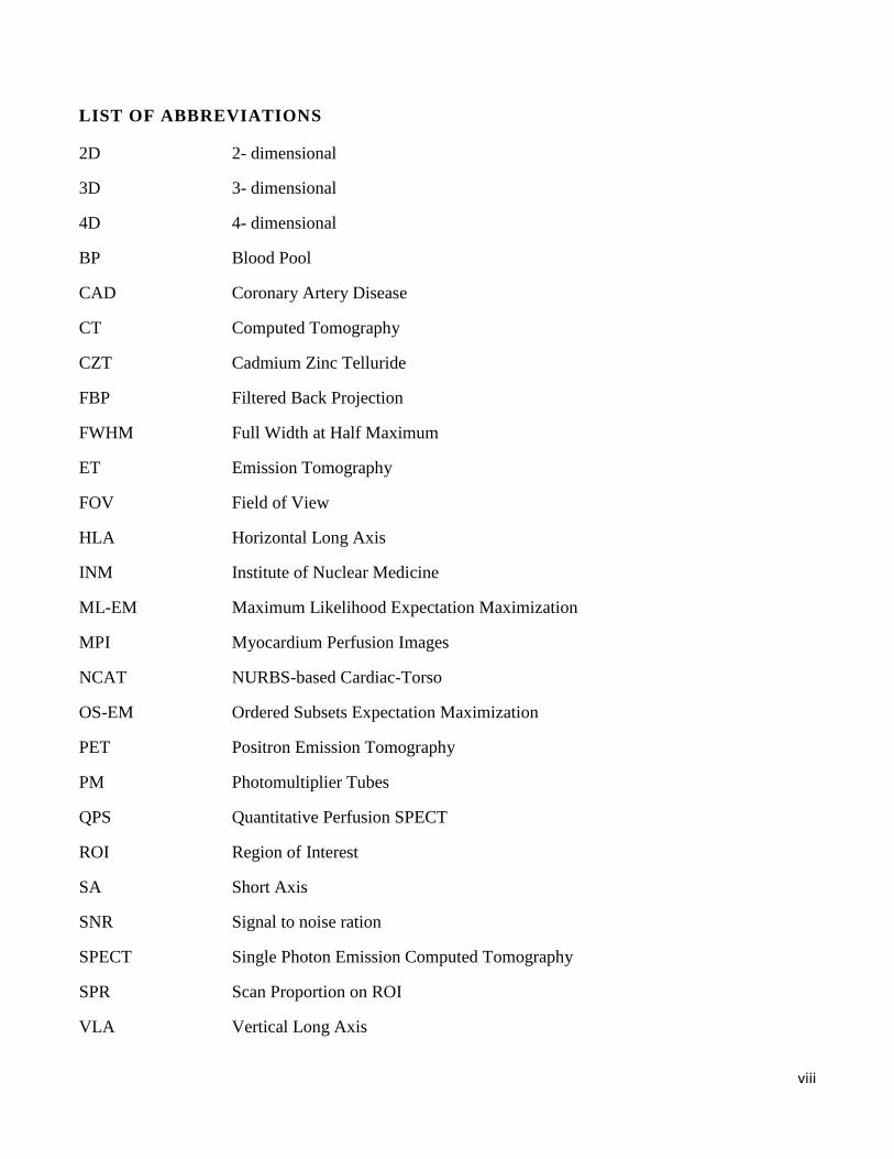
LIST OF ABBREVIATIONS
2D 2- dimensional
3D 3- dimensional
4D
BP
4- dimensional
Blood Pool
CAD
CT
Coronary Artery Disease
Computed Tomography
CZT Cadmium Zinc Telluride
FBP
FWHM
ET
Filtered Back Projection
Full Width at Half Maximum
Emission Tomography
FOV Field of View
HLA
INM
Horizontal Long Axis
Institute of Nuclear Medicine
ML-EM Maximum Likelihood Expectation Maximization
MPI
NCAT
Myocardium Perfusion Images
NURBS-based Cardiac-Torso
OS-EM Ordered Subsets Expectation Maximization
PET
PM
QPS
ROI
Positron Emission Tomography
Photomultiplier Tubes
Quantitative Perfusion SPECT
Region of Interest
SA
SNR
SPECT
SPR
VLA
Short Axis
Signal to noise ration
Single Photon Emission Computed Tomography
Scan Proportion on ROI
Vertical Long Axis
ix
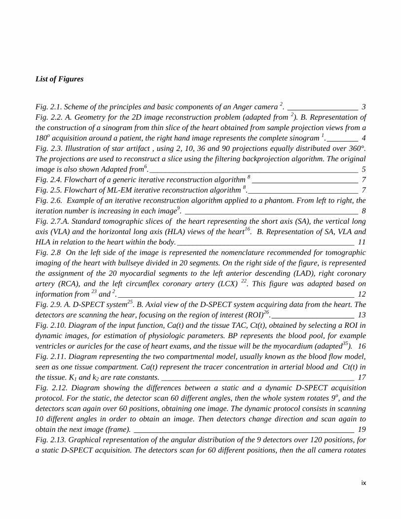
List of Figures
Fig. 2.1. Scheme of the principles and basic components of an Anger camera 2. __________________ 3
Fig. 2.2. A. Geometry for the 2D image reconstruction problem (adapted from 2). B. Representation of
the construction of a sinogram from thin slice of the heart obtained from sample projection views from a
180o acquisition around a patient, the right hand image represents the complete sinogram
1. ________ 4
Fig. 2.3. Illustration of star artifact , using 2, 10, 36 and 90 projections equally distributed over 360°.
The projections are used to reconstruct a slice using the filtering backprojection algorithm. The original
image is also shown Adapted from6. _____________________________________________________ 5
Fig. 2.4. Flowchart of a generic iterative reconstruction algorithm 8 ___________________________ 7
Fig. 2.5. Flowchart of ML-EM iterative reconstruction algorithm 8. ____________________________ 7
Fig. 2.6. Example of an iterative reconstruction algorithm applied to a phantom. From left to right, the
iteration number is increasing in each image9. ____________________________________________ 8
Fig. 2.7.A. Standard tomographic slices of the heart representing the short axis (SA), the vertical long
axis (VLA) and the horizontal long axis (HLA) views of the heart16
. B. Representation of SA, VLA and
HLA in relation to the heart within the body. _____________________________________________ 11
Fig. 2.8 On the left side of the image is represented the nomenclature recommended for tomographic
imaging of the heart with bullseye divided in 20 segments. On the right side of the figure, is represented
the assignment of the 20 myocardial segments to the left anterior descending (LAD), right coronary
artery (RCA), and the left circumflex coronary artery (LCX) 22
. This figure was adapted based on
information from 23
and 2. ____________________________________________________________ 12
Fig. 2.9. A. D-SPECT system25
. B. Axial view of the D-SPECT system acquiring data from the heart. The
detectors are scanning the hear, focusing on the region of interest (ROI)26
. _____________________ 13
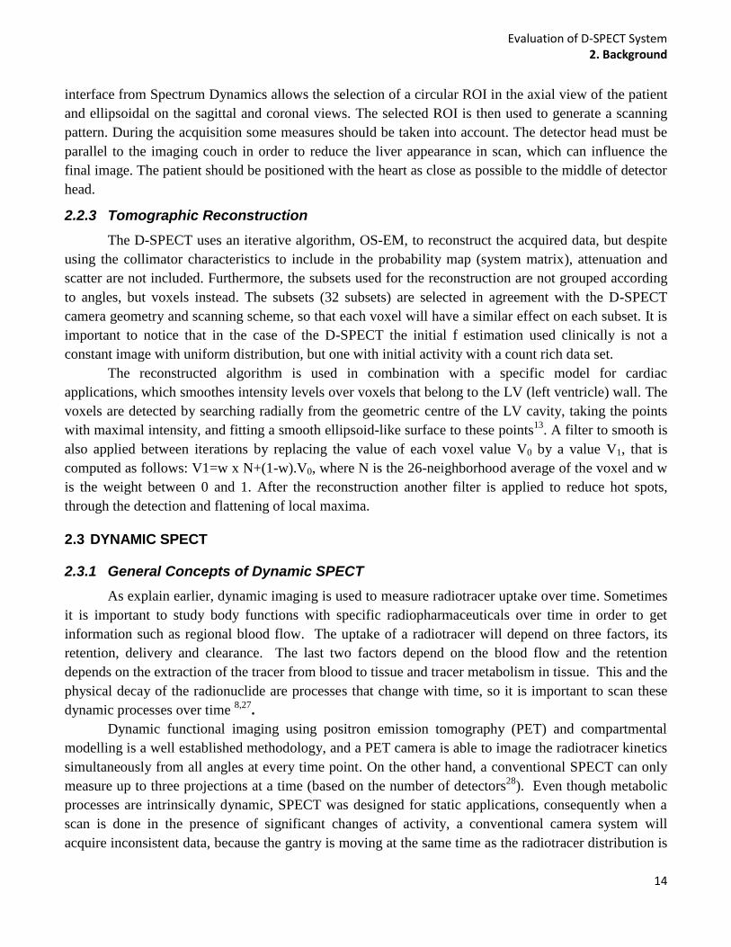
Fig. 2.10. Diagram of the input function, Ca(t) and the tissue TAC, Ct(t), obtained by selecting a ROI in
dynamic images, for estimation of physiologic parameters. BP represents the blood pool, for example
ventricles or auricles for the case of heart exams, and the tissue will be the myocardium (adapted35
). 16
Fig. 2.11. Diagram representing the two compartmental model, usually known as the blood flow model,
seen as one tissue compartment. Ca(t) represent the tracer concentration in arterial blood and Ct(t) in
the tissue. K1 and k2 are rate constants. _________________________________________________ 17
Fig. 2.12. Diagram showing the differences between a static and a dynamic D-SPECT acquisition
protocol. For the static, the detector scan 60 different angles, then the whole system rotates 9o, and the
detectors scan again over 60 positions, obtaining one image. The dynamic protocol consists in scanning
10 different angles in order to obtain an image. Then detectors change direction and scan again to
obtain the next image (frame). ________________________________________________________ 19
Fig. 2.13. Graphical representation of the angular distribution of the 9 detectors over 120 positions, for
a static D-SPECT acquisition. The detectors scan for 60 different positions, then the all camera rotates
x
9o, showed by the decreased angular value, and then a new scan is done for the remaining 60 positions.
_________________________________________________________________________________ 24
Fig. 2.14. The three different algorithms available in the model simulator used to calculate the scan
patterns. _________________________________________________________________________ 24
Fig. 2.15. Anterior view of the 4-D NCAT combined with models of imaging process, the phantom can
simulate emission and transmission imaging data47
. _______________________________________ 25
Fig. 3.1. Methodology diagram showing that to obtain the projections, both camera (created in
D_SPECT interface) and source (obtained with NCAT phantom program) are needed. Then both are
loaded on the simulator interface (zoomed representation of Fig. A in appendix section) in order to
calculate the projections. Then projections can be reconstructed and data analyzed. The diagram also
shows that different cameras are used while the source is always the same. _____________________ 27
Fig. 3.2. Interface to easily load, create and save ROIs _____________________________________ 28
Fig. 3.3. Transaxial view of the heart A. two different ROI positions, shifting up and left, and B. three
different ROI sizes selected for the study, the original, the bigger and a smaller ROI. _____________ 29
Fig. 3.4. Scheme of the four different scan patterns created. For Open sweep the whole FOV is scanned,
the Clinical represent the scan pattern performed by D-SPECT clinically, where a ROI is defined and
the detectors spend around 60% of the time scanning inside the ROI and the remaining time on the rest
of the FOV. ROI only, only the ROI is scanned using detector leading edge algorithm to calculate the
projections while for the small ROI the detector trailing edge was the one applied._______________ 31
Fig. 3.5. Clinical transverse, coronal and sagittal views of the LV of the heart for two different scan
patterns, taken from AMIDE. The initial ROI represents the ROI where the heart is on the centre of the
region and the size of it corresponds to the first simulation. _________________________________ 32
Fig. 3.6. Reconstructed images for four different scan patterns. The left ventricle of the myocardium
seems to become thinner from data from left to right. Right ventricle and atria are not visible for the
small ROI scan patterns, and there are artefacts around the heart. ___________________________ 33
Fig. 3.7. Bullseye plots obtained from QPS for both clinical open sweep and small ROI. Each segment
represented has a value between 1 and 100, given a scale of intensity on that segment. ___________ 33
Fig. 3.8. Three slices of the short axis of the heart view for both open sweep and small ROI. The two
extreme slices of short axis were not represented when the projections were calculated with small ROI.
_________________________________________________________________________________ 34
Fig. 3.9. Plot of 14 inner rings segment values for open sweep and small ROI scan compared with the
values for each segment of the clinical scan. Respective R2 values are plotted. __________________ 34
Fig. 3.10. Mean activity in the left ventricle of the myocardium selected by a 3D mask based on
intensity, for all the four scan patterns (Open sweep, clinical, ROI only, small ROI). _____________ 36
Fig. 4.1. Methodology diagram showing that to obtain the projections, both camera (created in
D_SPECT interface) and source (obtained with NCAT phantom program) are needed. Both are loaded
on the interface (zoomed representation on Fig. A in appendix section) in order to calculate the
projections. Then projection can be reconstructed and data analyzed. The diagram also suggests the
camera used is always the same simulating a ROI only scan protocol, while several sources are used for
the simulations. ____________________________________________________________________ 37
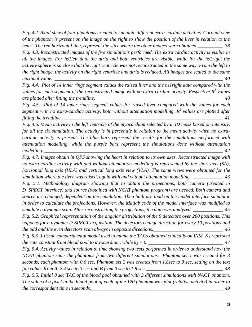
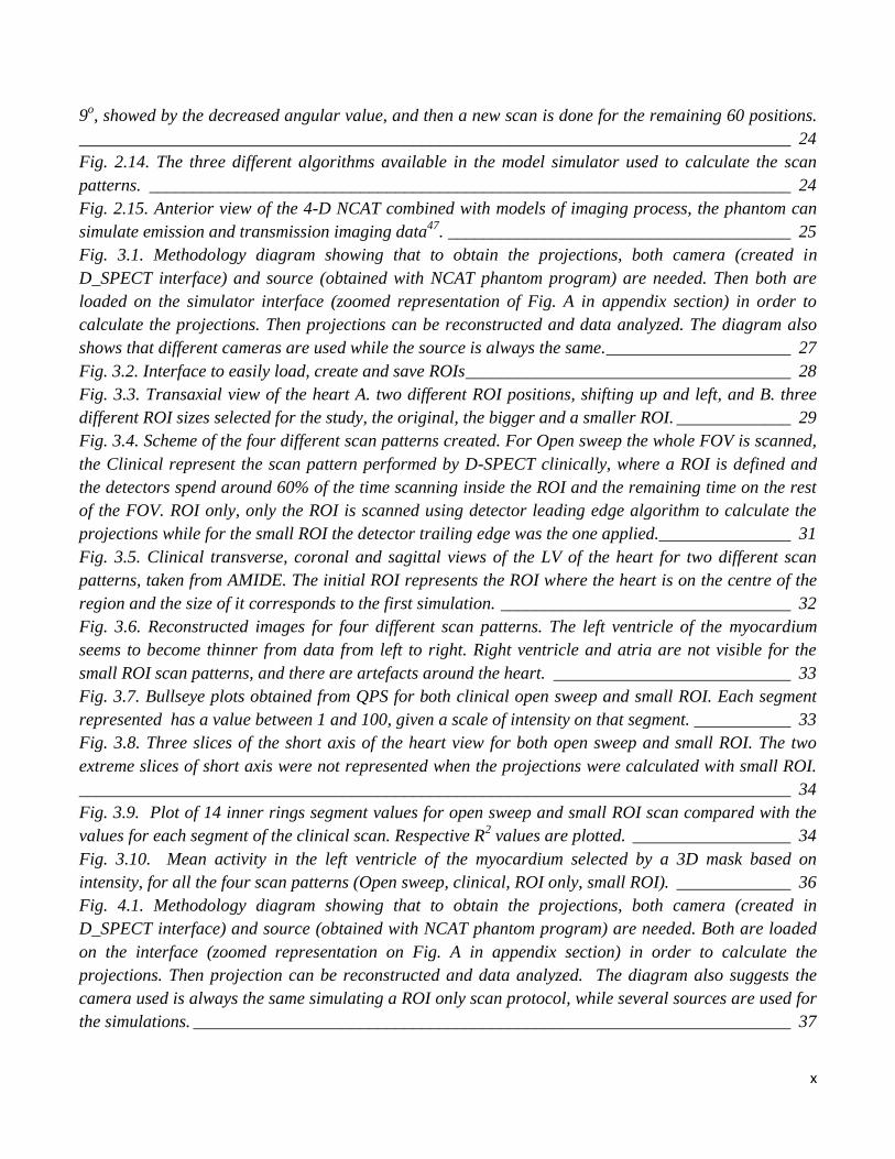
xi
Fig. 4.2. Axial slice of four phantoms created to simulate different extra-cardiac activities. Coronal view
of the phantom is present on the image on the right to show the position of the liver in relation to the
heart. The red horizontal line, represent the slice where the other images were obtained. __________ 38
Fig. 4.3. Reconstructed images of the five simulations performed. The extra cardiac activity is visible in
all the images. For hs1left data the atria and both ventricles are visible, while for the hs1right the
activity sphere is so close that the right ventricle was not reconstructed in the same way. From the left to
the right image, the activity on the right ventricle and atria is reduced. All images are scaled to the same
maximal value. ____________________________________________________________________ 40
Fig. 4.4. Plot of 14 inner rings segment values the raised liver and the hs1right data compared with the
values for each segment of the reconstructed image with no extra-cardiac activity. Respective R2 values
are plotted after fitting the trendline. ___________________________________________________ 40
Fig. 4.5. Plot of 14 inner rings segment values for raised liver compared with the values for each
segment with no extra-cardiac activity, both without attenuation modelling. R2 values are plotted after
fitting the trendline. _________________________________________________________________ 41
Fig. 4.6. Mean activity in the left ventricle of the myocardium selected by a 3D mask based on intensity,
for all the six simulation. The activity is in percentile in relation to the mean activity when no extra-
cardiac activity is present. The blue bars represent the results for the simulations performed with
attenuation modelling, while the purple bars represent the simulations done without attenuation
modelling. ________________________________________________________________________ 42
Fig. 4.7. Images obtain in QPS showing the heart in relation to its own axes. Reconstructed image with
no extra cardiac activity with and without attenuation modelling is represented by the short axis (SA),
horizontal long axis (HLA) and vertical long axis view (VLA). The same views were obtained for the
simulation where the liver was raised, again with and without attenuation modelling. ____________ 43
Fig. 5.1. Methodology diagram showing that to obtain the projections, both camera (created in
D_SPECT interface) and source (obtained with NCAT phantom program) are needed. Both camera and
source are changed, dependent on the simulation. Then both are load on the model interface simulator
in order to calculate the projections. However, the Matlab code of the model interface was modified to
simulate a dynamic scan. After reconstructing the projections, the data was analyzed. ____________ 45
Fig. 5.2. Graphical representation of the angular distribution of the 9 detectors over 200 positions. This
happens for a dynamic D-SPECT acquisition. The detectors change direction for every 10 positions and
the odd and the even detectors scan always in opposite directions. ____________________________ 46
Fig. 5.3. 1 tissue compartmental model used to mimic the TACs obtained clinically on INM. K1 represent
the rate constant from blood pool to myocardium, while k2 = 0. ______________________________ 47
Fig. 5.4. Activity values in relation to time showing two tests performed in order to understand how the
NCAT phantom sums the phantoms from two different simulations. Phantom set 1 was created for 3
seconds, each phantom with 0.6 sec. Phantom set 2 was creates from 1.8sec to 3 sec, setting on the text
file values from A. 2.4 sec to 3 sec and B from 0 sec to 1.8 sec._______________________________ 48
Fig. 5.5. Initial 8 sec TAC of the blood pool obtained with 3 different simulations with NACT phantom.
The value of a pixel in the blood pool of each of the 120 phantom was plot (relative activity) in order to
the correspondent time in seconds. _____________________________________________________ 49
xii
Fig. 5.6. TACs for blood pool (bolus injection), liver and myocardium obtained by selecting a pixel
values for each organ in 480 different phantoms, simulation a 72 sec scan. _____________________ 50
Fig. 5.7. Diagram of the process used to obtain the simulated dynamic data and the reference data. For
each created frame the correspondent 10 phantoms are used to simulate the changes of activity over
time. The projections for all 10 positions of the camera are calculated for each phantom, but only the
simulated projections calculated with the phantom and the detectors on the right position are chosen.
The referenced data used only one phantom to obtain each frame, being that phantom the mean value of
the 10 phantoms used in the simulated dynamic data. For the 10 different views, the detectors will
always see the same phantom. After the selection of projections the same number of frames is obtained
and the data compared with TACs and K1 values. _________________________________________ 51
Fig. 5.8. Representation of the projections selected to create a 3 sec/frame scan, using the saved
projections calculated to create de 1.5 sec/frame scan. The first table represent the available saved
projection needed to create the first frame of 1.5sec/frame scan, being associated with camera A. The
shadowed columns represent the selected the direct sampling selection while the right symbols represent
the selected projection. The second table represent the same but for frame 2 of 1.5 sec/frame, being the
camera B associated with the projections. _______________________________________________ 53
Fig. 5.9. Six different injection rates obtained selecting a pixel value on the blood pool of several
phantoms. Each curve represents a pixel value on the blood pool for several phantoms, for six different
sets of phantoms. Each set of phantom represent different injection rates, from rate 1 (slowest) to rate 6
(faster). __________________________________________________________________________ 55
Fig. 5.10. Diagram representing how the data was organized in order to make a quantitative and
qualitative analysis of the resultant reconstructed images. __________________________________ 58
Fig. 5.11. Location of the blood pool and myocardium VOIs (based on intensity) in a slice of the
reconstructed data, selected to create TACs. _____________________________________________ 59
Fig. 5.12. Axial slice of the heart for all the frames obtained with the dynamic scan data, for injection
rate 3 and scan sampling of 3 sec/frame, over 18 sec (0.3sec * 16frames). The images are scaled to the
maximal value of the correspondent frames obtained with the reference data. ___________________ 61
Fig. 5.13. Axial slice of the heart for all the frames obtained with reference scan data, for injection rate
3 and scan sampling of 3 sec/frame, over 18 sec (0.3sec * 16frames). _________________________ 61
Fig. 5.14. Dynamic scan data: Axial slice of all the frames obtained with the 4 scan samplings over 12
seconds for injection rate 3. On the right side are represented the TACs from dynamic data (red) and
TACs from reference data (blue) plotted with information from all frames obtained during the scan
time, selecting VOIs on both blood pool (input function) and myocardium. _____________________ 62
Fig. 5.15. Reference scan data: Axial slice of all the frames obtained with the 4 scan samplings over 12
seconds for injection rate 3. On the right side are represented the TACs from dynamic data (red) and
TACs from reference data (blue) plotted with information from all frames obtained during the scan time,
selecting VOIs on both blood pool (input function) and myocardium. __________________________ 63
Fig. 5.16. Dynamic scan data: Axial slice of all the frames obtained with the 4 scan samplings over 12
seconds for injection rate 5. On the right side are represented the TACs from dynamic data (red) and
xiii
TACs from reference data (blue) plotted with information from all frames obtained during the scan time,
selecting VOIs on both blood pool (input function) and myocardium. __________________________ 64
Fig. 5.17. Reference scan data: Axial slice of all the frames obtained with the 4 scan samplings over 12
seconds for injection rate 5. On the right side are represented the TACs from dynamic data (red) and
TACs from reference data (blue) plotted with information from all frames obtained during the scan time,
selecting VOIs on both blood pool (input function) and myocardium. __________________________ 64
Fig. 5.18. Maximum value of the absolute difference between each point of the TACs obtained with
dynamic scan data and reference data, for an open sweep scan. The Maximum value is plot for 5
injection rates and respective scan samplings. ____________________________________________ 65
Fig. 5.19. Maximum value of absolute difference between each point of the TACs obtained with dynamic
scan data and reference data, for an ROI only scan. The Maximum value is plot for 5 injection rates and
respective scan samplings. ___________________________________________________________ 66
Fig. 5.20. The ratio values between the obtained K1 for reference image (referred as K1 average) and
the K1 obtained with dynamic scan , for the 5 injection rates and respective scan samplings. _______ 67
Fig. 5.21. Maximum value of the absolute difference between each point of the TACs obtained with
dynamic scan data and reference data, for an open sweep scan, after interpolation of values for
3sec/frame, 6 sec/frame and 12sec/frame. The Maximum value is plot for 5 injection rates and
respective scan samplings. ___________________________________________________________ 67
Fig. 5.22. Dynamic scan data: Axial slice of all the frames obtained with the 4 scan samplings over 12
seconds for injection rate 5, simulated with noise. Representation of TACs from dynamic data (red) and
TACs from reference data (blue) plotted with information from all frames obtained during the scan time,
selecting VOIs on both blood pool (input function) and myocardium __________________________ 68
Fig. 5.23. Reference scan data: Axial slice of all the frames obtained with the 4 scan samplings over 12
seconds for injection rate 5 simulated with noise. Representation of TACs from dynamic data (red) and
TACs from reference data (blue) plotted with information from all frames obtained during the scan time,
selecting VOIs on both blood pool (input function) and myocardium. __________________________ 69
Fig. 5.24. Maximum value of absolute difference between each point of the TACs obtained with dynamic
scan data and reference data in the blood pool, for simulations with noise. The Maximum value is plot
for injection rate 2 and 5 and respective scan samplings. ___________________________________ 70
Fig. 5.25. Maximum value of absolute difference between each point of the TACs obtained with dynamic
scan data and reference data in the myocardium, for simulations with noise. The Maximum value is plot
for injection rate 2 and 5 and respective scan samplings. ___________________________________ 70
Evaluation of D-SPECT System 1. Introduction
1
1 INTRODUCTION
Single photon emission computed tomography (SPECT) is a nuclear medicine technique,
allowing the diagnosis of several diseases in the body, derived from physiology and cellular function. To
obtain a SPECT exam, a radiopharmaceutical is administered to a patient and 3D images of its
distribution in the body is acquired. SPECT is widely use in cardiac studies but the system has some
limitations. Thus, for more accurate diagnosis of cardiac function, D-SPECT was created. The system
uses a novel detector geometry and a reconstruction algorithm based on maximum likelihood
expectation maximization (ML-EM). The new system has 9 pixelated solid state detectors, mounted
vertically in 90º geometry (arranged in a curved configuration to conform to the shape of the left side of
the patient’s chest), crystals of cadmium zinc telluride and short wide-angle collimators made with
tungsten. Each detector rotates around its central axis with a pre-selected angular orientation and in
synchrony. D-SPECT also allows a region-centric acquisition. However, before each D-SPECT scan, it
is essential to make a quick pre-scan to determine the position of the heart. With that image the ROI,
containing the heart, is selected manually. As a consequence, the system calculates a scanning pattern
according to the selected ROI, spending more time acquiring data from the region of interest (ROI) and
less from other body parts (normal acquisition). In addition D-SPECT also allows very fast dynamic
acquisition, what could be an advantage in relation to conventional SPECT systems. Nevertheless, each
of the 9 detectors is small and cannot see the whole heart at once, so there is a possibility to create
inconsistent projections. The analysis of dynamic nuclear medicine data comprises fitting models to
time-activity curves (TACs) generated from ROIs defined on a temporal sequence of reconstructed
images.
The objective of this work is to investigate if the new geometry of the D-SPECT camera as well
as the innovative region-centric acquisition of the data, can create any problems on the reconstructed
images. Static studies were performed in order to start understanding the limitations of the D-SPECT.
For instance, factors such as scanning pattern can be altered and may produce different reconstructed
images. Different scanning patterns can be obtained by defining different ROIs and choosing different
percentiles of time for the detectors to spend scanning the ROI. Defining different algorithms to
calculate the scan pattern may also produces changes on the reconstructed images. The presence of a
source of activity, near the heart, but outside the ROI, was also studied to verify how it influences the
reconstructed images. Since D-SPECT also allows scanning dynamic processes, the fact the
radiopharmaceutical activity is changing at the same time the detectors are moving to acquire the data,
was also assessed. Different protocols were study changing the temporal sampling to obtain each frame
and the rate of the radiopharmaceutical bolus injection.
To investigate the described situations a NURBS-based cardiac-torso (NCAT) phantom was used
in combination with a computer simulator tool, specifically design to simulated static D-SPECT
acquisitions. Modifications to the simulations had to be made in order to obtain projections obtained by
a dynamic acquisition. Then to visualize and analyze the obtained images different programs were used
including Matlab, AMIDE and Quantitative Perfusion SPECT (QPS).
Evaluation of D-SPECT System 1. Introduction
2
Relatively to the organization of the thesis, it was divided in five main chapters, including the
Background, three different studies performed, and the General Conclusion, the last chapter of the work.
Each of the three studies is divided in Aim, Materials and Methods, Results and Discussion, and
Conclusion. For a better understanding of the objectives of study and the theory underlined by the image
acquisition process, the Background chapter was divided in five subchapters. In the first subchapter a
brief introduction about the SPECT instrumentation is made including information about cardiac
SPECT. The way SPECT images are processed in terms of acquiring the data and obtaining projections,
as well as the reconstruction process is also explain on the same subchapter. In subchapter two a
comparison between D-SPECT and SPECT is done and the process from acquiring the data till the
images are reconstructed is explained for D-SPECT. The importance of dynamic SPECT is assessed in
another subchapter (subchapter three) where essential information is disclosed in order to clearly
understand the kinetic tracer study. In subchapter four the sources that degrade the reconstructed images
in nuclear medicine are explain, concerning that for all the simulation some image degradation factors
were modelling, so it is important to understand these affects. Further, the D-SPECT simulator is
described in subchapter five as well as the computer phantom used to simulate a source. In chapter three
the first project is explain, where the effects of different scan patterns are analyzed. Scan without ROI
and with different ROI are study in terms of artifacts on the reconstructed images. Chapter four is where
the effect of an activity spheres and the presence of a raised liver with higher activity than the heart,
outside the ROI is study, again in terms of the effects on the reconstructed images. The content of these
last two chapters was presented at the British Nuclear Medicine Society Spring Meeting 2012. The last
chapter is where the effects of tracer kinetics are studied. The importance of the study is explained as
well as the processing necessary to create simulations essential to understand the best acquisition
protocol.
Evaluation of D-SPECT System 2. Background
3
2 BACKGROUND
2.1 CONVENTIONAL SINGLE PHOTON EMISSION COMPUTED TOMOGRAPHY
2.1.1 General Concepts of SPECT System
Single photon emission computed tomography (SPECT) is a nuclear medicine technique used to
create cross-sectional diagnostic images. As in any other nuclear medicine exam, a radioactive material
is injected intravenously, inhaled or ingested by the patient. Nuclear medicine procedures create
functional images that are able to pinpoint molecular activity within the body and offer the potential to
identify disease in its earliest stages.
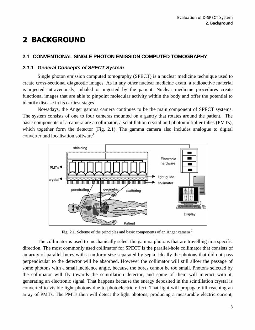
Nowadays, the Anger gamma camera continues to be the main component of SPECT systems.
The system consists of one to four cameras mounted on a gantry that rotates around the patient. The
basic components of a camera are a collimator, a scintillation crystal and photomultiplier tubes (PMTs),
which together form the detector (Fig. 2.1). The gamma camera also includes analogue to digital
converter and localisation software1.
Fig. 2.1. Scheme of the principles and basic components of an Anger camera 2.
The collimator is used to mechanically select the gamma photons that are travelling in a specific
direction. The most commonly used collimator for SPECT is the parallel-hole collimator that consists of
an array of parallel bores with a uniform size separated by septa. Ideally the photons that did not pass
perpendicular to the detector will be absorbed. However the collimator will still allow the passage of
some photons with a small incidence angle, because the bores cannot be too small. Photons selected by
the collimator will fly towards the scintillation detector, and some of them will interact with it,
generating an electronic signal. That happens because the energy deposited in the scintillation crystal is
converted to visible light photons due to photoelectric effect. That light will propagate till reaching an
array of PMTs. The PMTs then will detect the light photons, producing a measurable electric current,

Evaluation of D-SPECT System 2. Background
4
that is proportional to the number of the detected photons3. Since the objective is to determine the
distribution of the radiopharmaceutical within the body, it is important to know the position of the
interaction. That can be found from the light distribution. Then, dedicated electronics and software are
used to infer the likely point of impact of the gamma photon based on the output of each PMT in the
array.
2.1.2 Image Acquisition and Projections
The acquisition protocols in SPECT have the aim of measuring a sufficient number of
projections for tomographic reconstruction. To achieve this, the standard SPECT system has a gantry,
where the detectors are attached, which rotates around the patient. The acquisition can be done in
different ways: step-and-shoot mode, continuous and continuous step-and-shoot. The most commonly
used mode is the step-and-shoot, where the detectors (gantry) move at discrete angles along the circular
path.
Fig. 2.2. A. Geometry for the 2D image reconstruction problem (adapted from
2). B. Representation of the construction of a
sinogram from thin slice of the heart obtained from sample projection views from a 180o acquisition around a patient, the
right hand image represents the complete sinogram 1.
As previously mentioned the collimator is used to select the photons so that only those that are
parallel to the collimator holes will reach the detector. For each detector angle θ and each location s (s
passes perpendicular to the direction of the rays (Fig. 2.2)), the detector is defined by a line given by the
equation:
s = x cos θ + y sin θ Eq. 2.1
For a better comprehension of the reconstruction it is important to understand first the
projections. Radon defined the projection operator saying that the counts acquired over a specific
projection bin, g(s,θ), is the integral of the tracer activity along the line that passes through the object
(patient), that is perpendicular to the detector in the case of SPECT. It is mathematically convenient to
formulate the problem in terms of the rotated coordinate system (s,t). f(x,y) is the value estimated after
the reconstruction, because it gives the number of counts due to the tracer activity 4. Fig. 2.2 describes
the 2D geometrical configuration of the reconstruction problem. In this system the origin coincides with
A B

Evaluation of D-SPECT System 2. Background
5
the origin in the unrotated (x,y) system and the (s,t) axes are perpendicular and parallel, respectively, to
the projection array. After the acquisition of all the projections, they are subdivided by taking all the
projections for a single, thin slice of the patient, at a time. All the projections for each slice are then
ordered into an image called a sinogram.
The projection operation can be defined as a matrix product given by:
Eq. 2.2
where H is the projection operator, that allows to find the sinogram given the slice, and f and g
were already defined. A sinogram is created if the acquired data is rebind in a single plot so that the bin
projections are represented on the horizontal axis and the projection angles on the vertical axis. So a
sinogram is essentially a stack of the acquired projection views for angles from 0 o
to 180o (or 360
o).
This is applied for the case of SPECT images, where all of the rows in the sinogram came from the same
axial (y) position as can be seen in Fig. 2.2. B5.
It is also important to mention that in theory, the Eq. 2.2 can be solved by direct methods.
However, due to the noise in the projection, the matrix H is ill-conditioned, so the direct methods are not
employed to tomographic reconstruction1.
2.1.3 Tomographic Reconstruction
Since direct methods are not used to solve the Eq. 2.2 to determinate the 3D distribution of the
radiotracer from the projections acquired, different methods are applied. Nowadays the reconstructing
process can be done using two different approaches in order to solve the referred problem. One can use
analytic methods or iterative methods.
2.1.3.1 Analytic Methods
It is possible to visualize the analytical reconstruction considering that the number of photons
recorded in any given detector bin, represent the sum of contributions from the activity located along a
line perpendicular to the detector surface. That line represents the direction from which the photons
originate (in perfect conditions). One way to reconstruct an image is by backprojection, meaning
redistribute the collected counts over the contributing individual pixels that lie along the path of the rays
in the reconstruction matrix. The activity distribution is obtained if this process is repeated for each
projection element and for each angle that is acquired6.
Fig. 2.3. Illustration of star artifact , using 2, 10, 36 and 90 projections equally distributed over 360°. The projections are used
to reconstruct a slice using the filtering backprojection algorithm. The original image is also shown Adapted from6.
Evaluation of D-SPECT System 2. Background
6
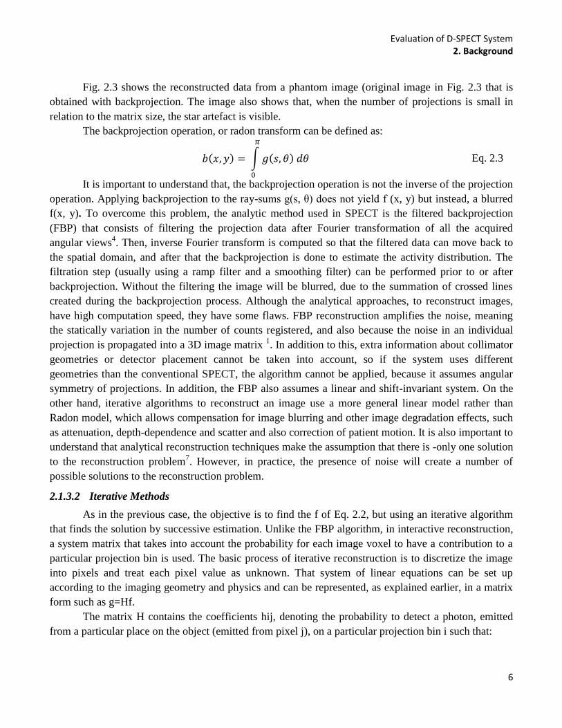
Fig. 2.3 shows the reconstructed data from a phantom image (original image in Fig. 2.3 that is
obtained with backprojection. The image also shows that, when the number of projections is small in
relation to the matrix size, the star artefact is visible.
The backprojection operation, or radon transform can be defined as:
Eq. 2.3
It is important to understand that, the backprojection operation is not the inverse of the projection
operation. Applying backprojection to the ray-sums g(s, θ) does not yield f (x, y) but instead, a blurred
f(x, y). To overcome this problem, the analytic method used in SPECT is the filtered backprojection
(FBP) that consists of filtering the projection data after Fourier transformation of all the acquired
angular views4. Then, inverse Fourier transform is computed so that the filtered data can move back to
the spatial domain, and after that the backprojection is done to estimate the activity distribution. The
filtration step (usually using a ramp filter and a smoothing filter) can be performed prior to or after
backprojection. Without the filtering the image will be blurred, due to the summation of crossed lines
created during the backprojection process. Although the analytical approaches, to reconstruct images,
have high computation speed, they have some flaws. FBP reconstruction amplifies the noise, meaning
the statically variation in the number of counts registered, and also because the noise in an individual
projection is propagated into a 3D image matrix 1. In addition to this, extra information about collimator
geometries or detector placement cannot be taken into account, so if the system uses different
geometries than the conventional SPECT, the algorithm cannot be applied, because it assumes angular
symmetry of projections. In addition, the FBP also assumes a linear and shift-invariant system. On the
other hand, iterative algorithms to reconstruct an image use a more general linear model rather than
Radon model, which allows compensation for image blurring and other image degradation effects, such
as attenuation, depth-dependence and scatter and also correction of patient motion. It is also important to
understand that analytical reconstruction techniques make the assumption that there is -only one solution
to the reconstruction problem7. However, in practice, the presence of noise will create a number of
possible solutions to the reconstruction problem.
2.1.3.2 Iterative Methods
As in the previous case, the objective is to find the f of Eq. 2.2, but using an iterative algorithm
that finds the solution by successive estimation. Unlike the FBP algorithm, in interactive reconstruction,
a system matrix that takes into account the probability for each image voxel to have a contribution to a
particular projection bin is used. The basic process of iterative reconstruction is to discretize the image
into pixels and treat each pixel value as unknown. That system of linear equations can be set up
according to the imaging geometry and physics and can be represented, as explained earlier, in a matrix
form such as g=Hf.
The matrix H contains the coefficients hij, denoting the probability to detect a photon, emitted
from a particular place on the object (emitted from pixel j), on a particular projection bin i such that:
Evaluation of D-SPECT System 2. Background
7
Eq. 2.4
The projection space is discrete and the vector g represents the projection data, where each
projection is represented by a bin 6. The activity distribution is given by f. Any element of the image,
referred to as a pixel, or a voxel, dependent on the dimension of the image. H is a matrix called the
system matrix that describes the imaging process. Attenuation and any linear blurring effect can be
included in the system matrix.
So the problem of reconstruction can be visualized as a way to find the object distribution f, from
the measured projections g, as mentioned, but also from information about the imaging system (system
matrix) and statistical description of the data and object. But to initialize the process it is essential to
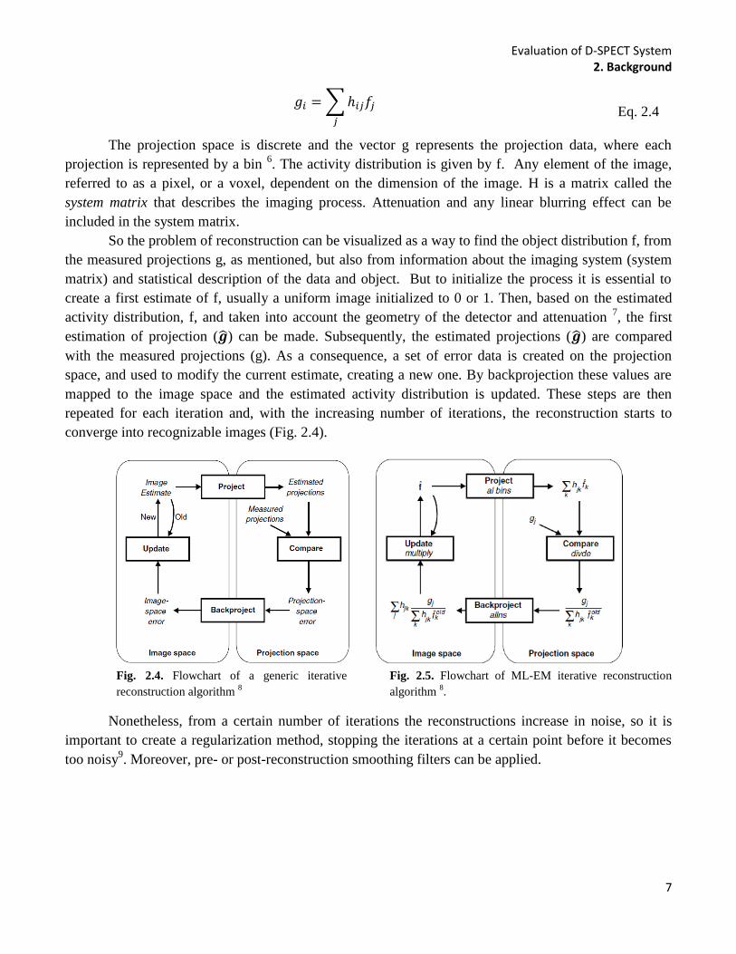
create a first estimate of f, usually a uniform image initialized to 0 or 1. Then, based on the estimated
activity distribution, f, and taken into account the geometry of the detector and attenuation 7, the first
estimation of projection ( ) can be made. Subsequently, the estimated projections ( ) are compared
with the measured projections (g). As a consequence, a set of error data is created on the projection
space, and used to modify the current estimate, creating a new one. By backprojection these values are
mapped to the image space and the estimated activity distribution is updated. These steps are then
repeated for each iteration and, with the increasing number of iterations, the reconstruction starts to
converge into recognizable images (Fig. 2.4).
Fig. 2.4. Flowchart of a generic iterative
reconstruction algorithm 8
Fig. 2.5. Flowchart of ML-EM iterative reconstruction
algorithm 8.
Nonetheless, from a certain number of iterations the reconstructions increase in noise, so it is
important to create a regularization method, stopping the iterations at a certain point before it becomes
too noisy9. Moreover, pre- or post-reconstruction smoothing filters can be applied.
Evaluation of D-SPECT System 2. Background
8
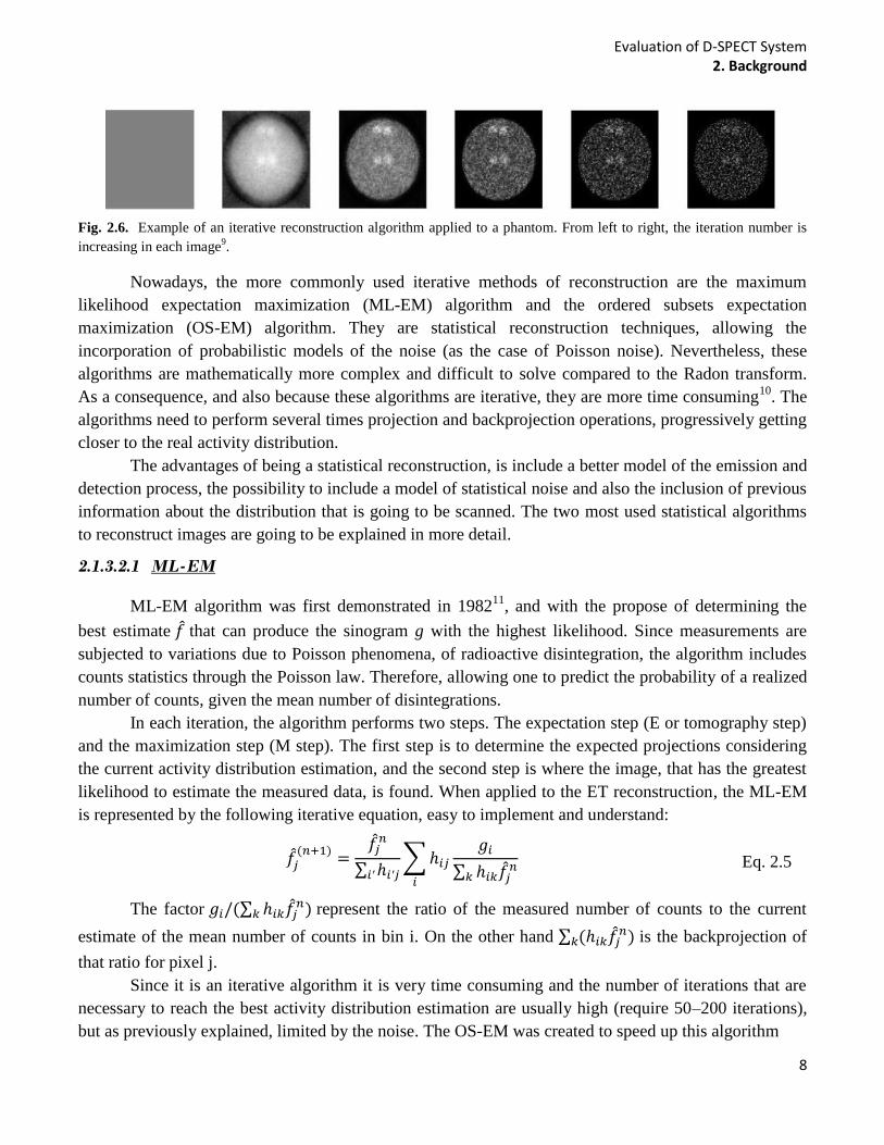
Fig. 2.6. Example of an iterative reconstruction algorithm applied to a phantom. From left to right, the iteration number is
increasing in each image9.
Nowadays, the more commonly used iterative methods of reconstruction are the maximum
likelihood expectation maximization (ML-EM) algorithm and the ordered subsets expectation
maximization (OS-EM) algorithm. They are statistical reconstruction techniques, allowing the
incorporation of probabilistic models of the noise (as the case of Poisson noise). Nevertheless, these
algorithms are mathematically more complex and difficult to solve compared to the Radon transform.
As a consequence, and also because these algorithms are iterative, they are more time consuming10
. The
algorithms need to perform several times projection and backprojection operations, progressively getting
closer to the real activity distribution.
The advantages of being a statistical reconstruction, is include a better model of the emission and
detection process, the possibility to include a model of statistical noise and also the inclusion of previous
information about the distribution that is going to be scanned. The two most used statistical algorithms
to reconstruct images are going to be explained in more detail.
2.1.3.2.1 ML-EM
ML-EM algorithm was first demonstrated in 198211
, and with the propose of determining the
best estimate that can produce the sinogram g with the highest likelihood. Since measurements are
subjected to variations due to Poisson phenomena, of radioactive disintegration, the algorithm includes
counts statistics through the Poisson law. Therefore, allowing one to predict the probability of a realized
number of counts, given the mean number of disintegrations.
In each iteration, the algorithm performs two steps. The expectation step (E or tomography step)
and the maximization step (M step). The first step is to determine the expected projections considering
the current activity distribution estimation, and the second step is where the image, that has the greatest
likelihood to estimate the measured data, is found. When applied to the ET reconstruction, the ML-EM
is represented by the following iterative equation, easy to implement and understand:
Eq. 2.5
The factor
represent the ratio of the measured number of counts to the current
estimate of the mean number of counts in bin i. On the other hand
is the backprojection of
that ratio for pixel j.
Since it is an iterative algorithm it is very time consuming and the number of iterations that are
necessary to reach the best activity distribution estimation are usually high (require 50–200 iterations),
but as previously explained, limited by the noise. The OS-EM was created to speed up this algorithm
Evaluation of D-SPECT System 2. Background
9
2.1.3.2.2 OS-EM
OS-EM is an accelerated version of ML-EM and instead of using all the data to obtain an update
of the reconstructed images, as the case of ML-EM, each iteration is made after one subset is used.
Subsets are small groups of projections data with equally, not contiguous, number of projections. As a
result, OS-EM algorithm is just a simple modification of the ML-EM given by the equation:
Eq. 2.6
Using subsets in each iteration, and not all projection, was proved to produce very similar results
to ML-EM algorithm, but much faster12
. In this case the backprojections are performed just for the
projection bins that belong to subset Sn, and in each update a different subset is used. The organization
of the subsets is important to the performance of the algorithm. For example, if one subset has stored
data from projections number 1, 9, 18, and so on, the data from the following subset could contain data
from projections 2, 10, 19 and the same happens for the other subsets6. The application on each subset of
the EM reconstruction is done one by one and so that the resulting reconstruction from subset 1 will be
the starting point of subset 2 and so on. Consequently, OSEM converges to the same point as MLEM,
but it needs less number of iterations (number of ML-EM iterations divided by the number of subsets).
2.1.4 Cardiac SPECT
SPECT is widely used clinically to diagnose several diseases, including cardiac studies, such as
myocardial perfusion imaging (MPI). Most SPECT studies are performed using a conventional dual-
head camera, configured in 90o degree geometry to scan the heart, in order to make MPI, taking around
15 to 20 minutes. The time spent for the scanning is necessary to create a good image with adequate
statistics, but sometimes artifacts are created due to patient motion13
. As previously mention, PMTs are
essential to enhance signal amplitude and the collimator essential to select the photon providing an
image with good spatial resolution, however with great cost in sensitivity. The trade-off between
resolution and sensitivity determines the performance of conventional gamma cameras. Limitations in
sensitivity result in long imaging times and relatively high doses of radiopharmaceuticals.
In order to overcome these problems new cameras dedicated to cardiac SPECT images were
created. The collimator design and the reconstructed algorithm were improved and new detectors and
gantry geometries arose. One of the created systems is D-SPECT from Spectrum Dynamics (Caesarea,
Israel) that allows high-speed perfusion imaging14,15
.
2.1.4.1 Myocardial Perfusion Imaging
MPI is the most widely employed non-invasive test used routinely for diagnosing and assessing
coronary artery disease (CAD) and other hear diseases, measuring the blood flow16,17
. CAD occurs when
arteries become hardened and narrowed, leading to failure of coronary circulation. MPI SPECT images
provide a visual 3D image of the perfused myocardium and are usually gated by the electrocardiogram
(ECG) in order to make a functional assessment of the images. The radiopharmaceutical must have a
property that allows it to distribute in the myocardium, proportionally to blood flow. On the other hand,
Evaluation of D-SPECT System 2. Background
10
even though the radiopharmaceutical should be swiftly eliminated, it also has to have a stable retention
within the myocardium during the exam time16
. To know the relative regional distribution of perfusion,
the MPI SPECT can be assessed at both rest and cardiovascular stress (injection of a vasoactive drug),
and usually the acquisition is made for both situations18
. A region with maximal uptake is assumed to
be normally perfused, and regions with significantly reduced uptake are interpreted as abnormally
perfused19
. Nowadays, the most accepted radionuclide is 99mTc, because it produces images with high
quality, resulting from high energy photon (140Kev) with relatively short half-life (6h).
2.1.4.2 Types of Data Acquisition: Static, Dynamic and Gated
SPECT acquisition has been considered to be applied just for static studies. These studies can be
seen as long-exposure photography, which means the reconstructed images will represent an average of
the radiotracer distribution over the total time of the acquisition. This type of acquisition can only be
done when the activity of the radiotracer is nearly constant, or when physiologically induced time
variations in the radiotracer distribution are very slow. Static acquisition mode is also performed when
the observation of the activity variations is not an important factor.
Besides static protocol, there are two main alternative acquisitions that create a sequence of
images that can be viewed as a movie, the dynamic and the gated acquisitions. Even though static
images are very useful to obtain perfusion images, little is being done in the last years to improve the
basic method of perfusion scintigraphy. No new radiopharmaceuticals were developed nor have new
hardware improvements been done. Nevertheless, dynamic cardiac SPECT has emerged as a good
option to improve risk stratification of cardiac problems17
. Static SPECT acquisition is very important,
because myocardium perfusion images can be obtained given information about tracer uptake. However,
very useful information about cardiac function can be obtained measuring the tracer uptake over time
that will allow the assessment of myocardium blood flow.
Dynamic imaging captures the distribution of a radiotracer over time, revealing information
about an organ physiology. Usually are used in visual assessments of organ function and are required for
most kinds of kinetic parameter estimation. These parameters describe dynamic behaviour of a tracer in
cardiac tissue, giving important clinical information20
. This matter will be discussed in more detail in the
section 2.3. Moreover, gated acquisition is a variation of dynamic imaging. Several images of an organ
in motion are acquired in synchronism with an electrocardiogram (ECG) signal. The acquired images
that started at the same time as the first part of the cardiac cycle are combined to form a composite of all
the cardiac cycles. In a similar way, all the successive obtained frames are formed through the
combination of all the counts acquired at a correspondent time interval in the cardiac cycle. So in gated
SPECT it is assumed a stationary distribution over the entire scan, while for a dynamic SPECT the
cardiac motion is typically ignored21
.
2.1.5 SPECT Post-reconstruction - Cardiac Image Processing
After the reconstruction process transaxial images are obtained, however if necessary sagittal,
coronal and oblique views can also be generated. By convention, the transaxial slices are oriented
perpendicular to the long axis of the body. Sagittal and coronal slices are oriented parallel to the long
axis of the body and at right angles to each other. This visualization can also be done for cardiac images,
Evaluation of D-SPECT System 2. Background
11
but for a better analysis of MPI images, instead of using the 2D transaxial slices to obtain sagittal or
coronal views, it is a common practice to reorient the slices. The axes of the heart can be defined in
relation to the heart’s long axis (line from base to apex). The horizontal long axis view (HLA) and
vertical long axis view (VLA) are oriented parallel to the long axis of the heart. The short axis (SA) is
also used and it is perpendicular to the long axis of the heart. All of these three views are oriented at 90o
angles to each other. These are usually used for the examination of coronary blood flow and evaluation
of left ventricular function2.
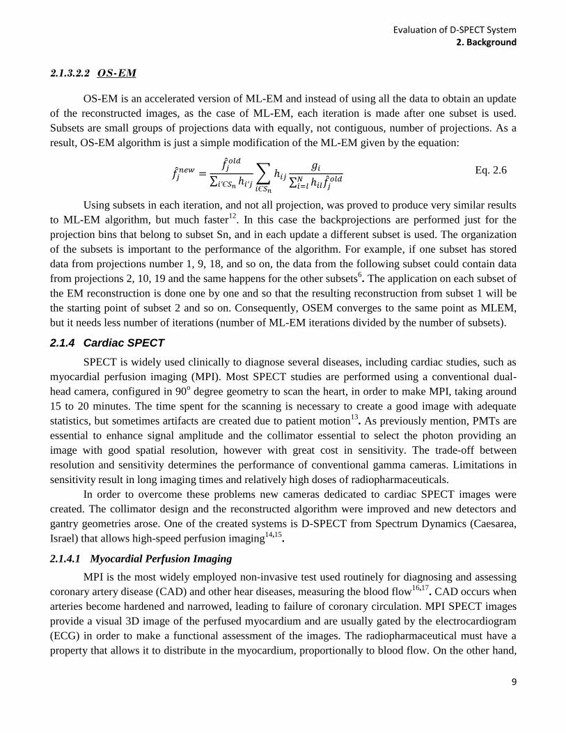
Reconstructed data from MPI SPECT are generally analysed visually, and usually the evaluation
is done using images from the described three views, SA, VLA and HLA, from rest and stress studies. In
a healthy perfused myocardium, the tracer distribution should be even throughout each slice. No regions
of reduce uptake or defects should appear.
Fig. 2.7.A. Standard tomographic slices of the heart representing the short axis (SA), the vertical long axis (VLA) and the
horizontal long axis (HLA) views of the heart16
. B. Representation of SA, VLA and HLA in relation to the heart within the
body.
Another way to visualize the heart is through a bullseye polar map. This type of visualization
allows the quantification of the 3D activity distribution within the myocardium, through the conversion
to a 2D polar map. The way the bullseye is made consists in modelling the myocardium into a new
system with cylindrical and spherical coordinates. Here the entire LV is displayed as a circular region,
with the apex of the ventricle at the centre and the base at the edge. This is then divided in segments (20
or 17 segments) in order to make it possible to compare the heart uptake in different regions of the
heart22
.
A B
Evaluation of D-SPECT System 2. Background
12
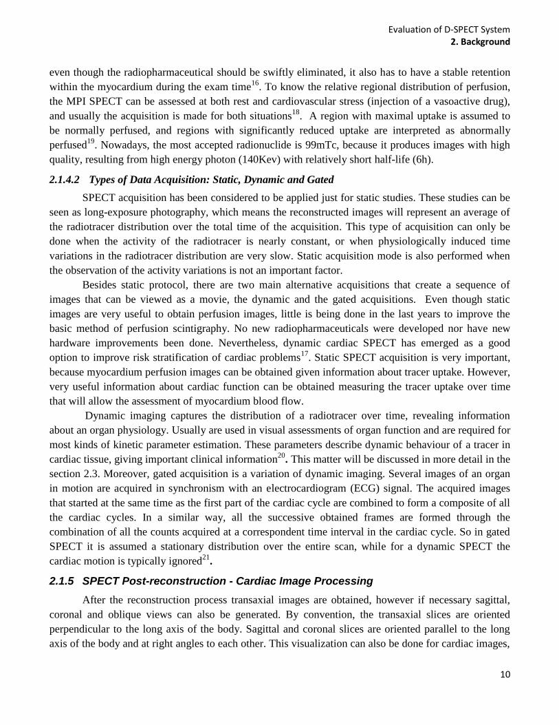
Fig. 2.8 On the left side of the image is represented the nomenclature recommended for tomographic imaging of the heart
with bullseye divided in 20 segments. On the right side of the figure, is represented the assignment of the 20 myocardial
segments to the left anterior descending (LAD), right coronary artery (RCA), and the left circumflex coronary artery (LCX) 22
. This figure was adapted based on information from 23
and 2.
Fig. 2.8 shows the location and the recommended names for the 20 myocardial segments in a
bullseye display. The names basal, mid-cavity, and apical are used to identify the location on the long
axis of the left ventricle.
2.2 D-SPECT SYSTEM
2.2.1 A Comparison with Conventional SPECT System
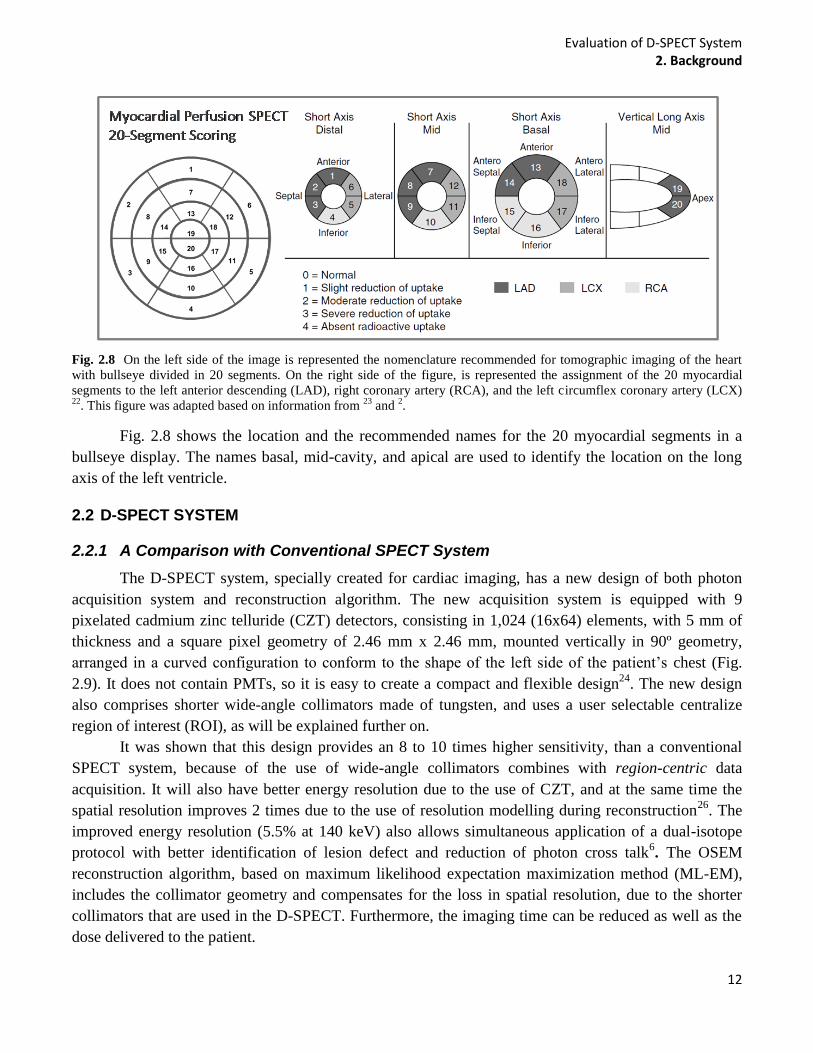
The D-SPECT system, specially created for cardiac imaging, has a new design of both photon
acquisition system and reconstruction algorithm. The new acquisition system is equipped with 9
pixelated cadmium zinc telluride (CZT) detectors, consisting in 1,024 (16x64) elements, with 5 mm of
thickness and a square pixel geometry of 2.46 mm x 2.46 mm, mounted vertically in 90º geometry,
arranged in a curved configuration to conform to the shape of the left side of the patient’s chest (Fig.
2.9). It does not contain PMTs, so it is easy to create a compact and flexible design24
. The new design
also comprises shorter wide-angle collimators made of tungsten, and uses a user selectable centralize
region of interest (ROI), as will be explained further on.
It was shown that this design provides an 8 to 10 times higher sensitivity, than a conventional
SPECT system, because of the use of wide-angle collimators combines with region-centric data
acquisition. It will also have better energy resolution due to the use of CZT, and at the same time the
spatial resolution improves 2 times due to the use of resolution modelling during reconstruction26
. The
improved energy resolution (5.5% at 140 keV) also allows simultaneous application of a dual-isotope
protocol with better identification of lesion defect and reduction of photon cross talk6. The OSEM
reconstruction algorithm, based on maximum likelihood expectation maximization method (ML-EM),
includes the collimator geometry and compensates for the loss in spatial resolution, due to the shorter
collimators that are used in the D-SPECT. Furthermore, the imaging time can be reduced as well as the
dose delivered to the patient.

Evaluation of D-SPECT System 2. Background
13
Fig. 2.9. A. D-SPECT system25
. B. Axial view of the D-SPECT system acquiring data from the heart. The detectors are
scanning the hear, focusing on the region of interest (ROI)26
.
2.2.2 Image Acquisition and Projections
In regards to the new D-SPECT geometry it is evident that D-SPECT acquires data will be
differently from conventional SPECT. The acquisition is made with the patient in a semi-reclining
position or in the supine position and then each of the 9 detectors is programmed to rotate around its
central axis with a pre-selected angular orientation. The scan process is different from a conventional
SPECT because there is no gantry that rotates around the patient (Fig. 2.9). This new geometry also has
a big advantage when a small organ, as the heart, need to be scanned. The D-SPECT has a central ROI,
that allows a region-centric acquisition, which means that the system is programmed to spend more time
acquiring data from the ROI and less on the other body parts 24
. In the case of SPECT acquisition, all the
pixels at a given gantry head position collect photons during the same time interval which means that,
contrary to D-SPECT, the collection time spent to scan the left ventricle (LV) is the same as that spent
on the other body parts that are not interesting to scan13
. In order to know which ROI should be
selected, a pre-scan is always done before each imaging process, to identify the position of the heart in
relation to the chest and also to set the angle limits of scanning for each detector 26
.
Then, during the acquisition, the 9 detectors will scan the whole FOV, but will spend more time
on the defined ROI. After that, the whole system rotates by 9o to fill sampling gaps and then the scan is
repeated. In the end 60 plus 60 projections are obtained by each detector. The movements of the 9
detectors can be independent of each other or synchronized (both in stepwise or continuously mode).
Also it is important to note that D-SPECT detectors do not scan all in the same direction, they scan
alternating clockwise and counter clockwise. So for the D-SPECT system, if detector number 2, 4, 6 and
8 scan clockwise the rest will scan in the other direction. The detectors can rotate up to 110o so that the
object of interests can be viewed from hundreds of different angles. The data are usually acquired
focusing on the ROI13
, but can also scan the all FOV or just the ROI. As in the case of a conventional
SPECT, the detected projections are stored in a sinogram.
2.2.2.1 Clinical D-SPECT Acquisition
As mentioned earlier, clinically a 30s pre-scan is performed to create a preliminary image of the
activity distribution. Then the nuclear medicine technician defines a ROI that should include the whole
heart, but not much else, paying special attention to the LV that must be in the FOV. The D-SPECT
Evaluation of D-SPECT System 2. Background
14
interface from Spectrum Dynamics allows the selection of a circular ROI in the axial view of the patient
and ellipsoidal on the sagittal and coronal views. The selected ROI is then used to generate a scanning
pattern. During the acquisition some measures should be taken into account. The detector head must be
parallel to the imaging couch in order to reduce the liver appearance in scan, which can influence the
final image. The patient should be positioned with the heart as close as possible to the middle of detector
head.
2.2.3 Tomographic Reconstruction
The D-SPECT uses an iterative algorithm, OS-EM, to reconstruct the acquired data, but despite
using the collimator characteristics to include in the probability map (system matrix), attenuation and
scatter are not included. Furthermore, the subsets used for the reconstruction are not grouped according
to angles, but voxels instead. The subsets (32 subsets) are selected in agreement with the D-SPECT
camera geometry and scanning scheme, so that each voxel will have a similar effect on each subset. It is
important to notice that in the case of the D-SPECT the initial f estimation used clinically is not a
constant image with uniform distribution, but one with initial activity with a count rich data set.
The reconstructed algorithm is used in combination with a specific model for cardiac
applications, which smoothes intensity levels over voxels that belong to the LV (left ventricle) wall. The
voxels are detected by searching radially from the geometric centre of the LV cavity, taking the points
with maximal intensity, and fitting a smooth ellipsoid-like surface to these points13
. A filter to smooth is
also applied between iterations by replacing the value of each voxel value V0 by a value V1, that is
computed as follows: V1=w x N+(1-w).V0, where N is the 26-neighborhood average of the voxel and w
is the weight between 0 and 1. After the reconstruction another filter is applied to reduce hot spots,
through the detection and flattening of local maxima.
2.3 DYNAMIC SPECT
2.3.1 General Concepts of Dynamic SPECT
As explain earlier, dynamic imaging is used to measure radiotracer uptake over time. Sometimes
it is important to study body functions with specific radiopharmaceuticals over time in order to get
information such as regional blood flow. The uptake of a radiotracer will depend on three factors, its
retention, delivery and clearance. The last two factors depend on the blood flow and the retention
depends on the extraction of the tracer from blood to tissue and tracer metabolism in tissue. This and the
physical decay of the radionuclide are processes that change with time, so it is important to scan these
dynamic processes over time 8,27
.
Dynamic functional imaging using positron emission tomography (PET) and compartmental
modelling is a well established methodology, and a PET camera is able to image the radiotracer kinetics
simultaneously from all angles at every time point. On the other hand, a conventional SPECT can only
measure up to three projections at a time (based on the number of detectors28
). Even though metabolic
processes are intrinsically dynamic, SPECT was designed for static applications, consequently when a
scan is done in the presence of significant changes of activity, a conventional camera system will
acquire inconsistent data, because the gantry is moving at the same time as the radiotracer distribution is

Evaluation of D-SPECT System 2. Background
15
changing29
. This will create projections that do not correspond to the right dynamic states of the source
because projections from different angles scan different tracer distributions. Since the traditional
reconstruction methods were not designed to account for dynamic data, reconstructed images usually
have artifacts, leading to biased parameters estimation30,31
. This problem is reduced considerably if the
cameras rotate faster, allowing scanning of a set of angular views in a sufficiently short period of time so
that the variation is very small32
, although, the scanners have mechanical limitations and generally they
cannot be very fast.
In order to obtain accurate measurement of myocardial perfusion, the dynamics of the radiotracer
is very important33
. To acquire dynamic data, the SPECT collects the data using one or more rotating
gamma cameras over a period of time, obtaining several images17
. In cardiac imaging, the first sign of
activity is in the right ventricle, and then goes to the left ventricle. Then with the progression of time the
activity starts to disappear from the blood pool of the ventricles and starts to be seen in the myocardial
wall surrounding the left ventricle, after passing through the lungs.
There are two different approaches that can be used to analyse the data based on kinetic
parameters estimation. Estimation can be done directly from the projections or using the reconstructed
images. Considering the propose of the study, only the second method is explained, since this is how the
parameters are calculated by D-SPECT.
2.3.2 Time - Activity Curves and Parameters Estimation
This information can be analysed with time-activity curves (TACs), after obtaining the dynamic
nuclear medicine images, and then quantitative analysis can be done through the calculation of
physiologic/biochemical parameters6. TACs can be obtained selecting information pixel by pixel or
grouping pixels, representing homogeneous structures in various regions of interest (ROI), or volumes
of interest (VOIs). In Fig. 2.10 are illustrated TACs for blood (BP) and tissue, through the calculation of
the mean activity in a specific ROI.
Using a single pixel is usually too noisy so the selection of ROI is usually necessary, because
the radioactivity of the pixels is averaged, allowing one to process the data with better statistical
properties and also to reduce computing time, since a low number of ROIs are analysed and not
thousand of pixels. However, noisy TACs create difficulties in the extraction of accurate parameters
without analysis strategies, so correction for physical effects such as attenuation and scatter are
essential2. Other reasons for low spatial resolution found in most perfusion studies include the fact they
are performed without cardiac gating, and the presence of respiratory and heart motion are also affecting
the results. Corrections for partial volume effects (PVE) and spillover may also be needed. PVE occurs
due to the contribution of information between adjacent image regions due to the limited spatial
resolution usually associated with PET or SPECT data34
. This will be explained in more detail in section
2.4. Moreover, the accuracy on the parameters determination is also influenced by the reduced activity
of the radiotracer.
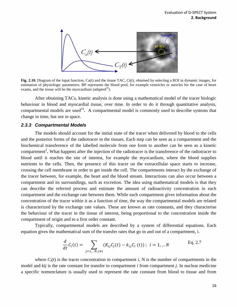
Evaluation of D-SPECT System 2. Background
16
Fig. 2.10. Diagram of the input function, Ca(t) and the tissue TAC, Ct(t), obtained by selecting a ROI in dynamic images, for
estimation of physiologic parameters. BP represents the blood pool, for example ventricles or auricles for the case of heart
exams, and the tissue will be the myocardium (adapted35
).
After obtaining TACs, kinetic analysis is done using a mathematical model of the tracer biologic
behaviour in blood and myocardial tissue, over time. In order to do it through quantitative analysis,
compartmental models are used33
. A compartmental model is commonly used to describe systems that
change in time, but not in space.
2.3.3 Compartmental Models
The models should account for the initial state of the tracer when delivered by blood to the cells
and the posterior forms of the radiotracer in the tissues. Each step can be seen as a compartment and the
biochemical transference of the labelled molecule from one form to another can be seen as a kinetic
compartment2. What happens after the injection of the radiotracer is the transference of the radiotracer to
blood until it reaches the site of interest, for example the myocardium, where the blood supplies
nutrients to the cells. Then, the presence of this tracer on the extracellular space starts to increase,
crossing the cell membrane in order to get inside the cell. The compartments interact by the exchange of
the tracer between, for example, the heart and the blood stream. Interactions can also occur between a
compartment and its surroundings, such as excretion. The idea using mathematical models is that they
can describe the referred process and estimate the amount of radioactivity concentration in each
compartment and the exchange rate between them. While each compartment gives information about the
concentration of the tracer within it as a function of time, the way the compartmental models are related
is characterized by the exchange rate values. These are known as rate constants, and they characterise
the behaviour of the tracer in the tissue of interest, being proportional to the concentration inside the
compartment of origin and to a first order constant.
Typically, compartmental models are described by a system of differential equations. Each
equation gives the mathematical sum of the transfer rates that go in and out of a compartment, i.
Eq. 2.7
where Ci(t) is the tracer concentration in compartment i, N is the number of compartments in the
model and kij is the rate constant for transfer to compartment i from compartment j. In nuclear medicine
a specific nomenclature is usually used to represent the rate constant from blood to tissue and from
Evaluation of D-SPECT System 2. Background
17
tissue to blood, being K1 and k2 respectively and any other additional rate constants to the model are
called k3, k4, ...ki. the unities of K1 are typically mL/min/mL while the other rate constants are
expressed in min-1
.
2.3.3.1 One Compartment Model - Flow
This is a simple compartmental model that is used for SPECT and PET applications, which
describes the bidirectional flux of the radiotracer between blood and tissue. The model given by Eq. 2.8,
is described by the Ct (t), the change of tracer concentration in tissue, and Ca(t) the change in the blood,
both over time.
Eq. 2.8
In order to obtain this equation it has to be assumed that for each compartment, for the blood and
the tissue, the radiotracer is homogeneously distributed. The unidirectional radiotracer flux from the
capillaries to tissue is given by K1Ca (wash-in) and the excretion from the tissue is given by k2Ci (wash-
out), as represented in Fig. 2.11.
Fig. 2.11. Diagram representing the two compartmental model, usually known as the blood flow model, seen as one tissue
compartment. Ca(t) represent the tracer concentration in arterial blood and Ct(t) in the tissue. K1 and k2 are rate constants.
Since, in most of the cases the tracer is removed from the blood via extraction to the tissues, the
blood concentration will decrease as it crosses the capillary walls. As a consequence, applying Ficks
law, the rate of change of a tracer concentration in tissue is proportional to blood flow and the difference
in the arterial and venous concentrations so that:
Eq. 2.9
In addition, the net fraction of the incoming tracer that goes from the blood to the tissue is called the
extraction fraction En and is given by:
Eq. 2.10
The non-directional extraction fraction (Eu), also known as first-pass extraction fraction, can just
be used to tracer what is extracted from blood to tissue8. In the beginning, for the first pass of the tracer
throughout a tissue site Ct will be zero. Therefore, in this stage En is equal to Eu and Eq. 2.8, Eq. 2.9 and
Eq. 2.10 can be arranged to give the net flux into tissue for the first pass.
Eq. 2.11
Evaluation of D-SPECT System 2. Background
18
The extraction fraction, Eu is also given by equation Eq. 2.12, that was calculated using the
Renkin-Crone capillary model, which assumes the capillary is a rigid cylindrical tube
Eq. 2.12
Where P gives the permeability value of the tracer across capillary membrane and S is the area of
the capillary surface while F represents the blood flow, and it is also dependent on time. Based on the
last two equations it is possible to verify that K1 is dependent on blood flow when the extraction fraction
is large, but is more dependent on permeability when extracellular fraction is small. Therefore, good
radiotracers are those with high extraction fraction. If it is assumed that the tracer concentration in tissue
is at equilibrium with that in venous blood the following assumption can be made.
Eq. 2.13
Consequently, Eq. 2.13 can be rewrite so that:
Eq. 2.14
Then, if F is replaced by FE in Eq. 2.14 and given that K1=FE and k2 = K1/VT, Eq. 2.8 is
obtained. Considering all these relations, one important application of these types of models is the fact
that we can measure a regional blood flow, F. Since it gives information about the volume of blood that
is passing through a blood vessel during time, it is a significant measure to be analysed clinically.
It is important to notice that the model represented in Fig. 2.11, even thou is usually represented
as a two compartment model is in really seen as having only one, because the TAC for blood is seen as
an input function and not a compartment, in a mathematical point of view. So, instead of calling it a two
compartmental model, the number of compartments is given by the number compartments that represent
a tissue. That is why the model is typically called one tissue compartmental model. In addition, the k2 is
commonly represented with an arrow from the tissue to the blood, however it does not correspond to the
actual mathematical relationship between the input and output functions6.
During a SPECT scan, it will measure the total activity on the field of view. This includes both
intra and extravascular activity. Thus in reality the concentration of activity measured by the scanner in
one voxel will be given by Ct* (t);
Eq. 2.15
VB is the fraction of measured volume that is occupied by blood, varying between 0 and 1 and
C*a(t) is the concentration of tracer in whole blood. This equation gives us the blood component in
tissue, and it is around 10-15% in the myocardium.

Evaluation of D-SPECT System 2. Background
19
2.3.4 Dynamic D-SPECT Acquisition and Reconstruction
As explained, D-SPECT allows MPI that is known to be useful in diagnosis of CAD. The
protocol used at the Institute of Nuclear Medicine at UCH to obtain dynamic images using D-SPECT is
well established and is being used for clinical studies. The protocol consists of a 60 seconds pre-scan
with the purpose of defining a ROI to be used in the main dynamic scan. In order to do it a dose of 40-
50MBq of 99m-Tc-MIBI is injected to the patient. It is important to notice that the image of the heart
will be very noisy due to the low activity injected and the short time of the scan, so the ROI adaptation
will be very dependent on the technician. After this, the remained dose (750-850MBq) is infused at a
rate of 5ml/min. During the process, the patient is imaged in a supine position, attached to a ‘Quickfit’
(MEDRAD) contrast injector filled with 100 mL saline, that is connected to a CT extension set and
MRI tubing, housed in a lead syringe box, that contain the dose. Then the rest protocol starts and
images are acquired during 6 minutes (6 sec/frame, 60 frames), immediately followed by a routine gated
SPECT for further more 6 min. This procedure is repeated for the dynamic stress acquisition where
adenosine is first injected and then, after two minutes, a bolus injection of 99m
Tc Sestamibi is infused
and flushed with 45 mL of saline. D-SPECT starts acquiring after 45 seconds before the bolus injection
in order to guarantee that the input function is not missed, since the D-SPECT systems takes some time
to start acquiring. ECG is used during all processes to monitor the patient.
The dynamic D-SPECT protocol is not equal to the static D-SPECT protocol in terms of data
acquisition, because instead of 60 different angular positions then the all system rotate 9o and then scan
again, the dynamic scan have to scan differently in order to obtain several images. Thus, instead of
obtaining all the projection to create one image, the dynamic acquisition takes only 10 projections per
detector to obtain each frame. So after a scan is completed for 10 different positions over the 110o angle
range of the D-SPECT system, the detectors invert direction and scan again (Fig. 2.12). In section 2.5.1,
the differences between the dynamic and the static D-SPECT scan patterns are explained in more detail.
Fig. 2.12. Diagram showing the differences between a static and a dynamic D-SPECT acquisition protocol. For the static, the detector scan 60 different angles, then the whole system rotates 9
o, and the detectors scan again over 60 positions,
obtaining one image. The dynamic protocol consists in scanning 10 different angles in order to obtain an image. Then detectors change direction and scan again to obtain the next image (frame).
All the images are then reconstructed with 4 Iterations and 32 subsets. Factor analysis is used to
create blood pool curves of the RV and LV and also for the myocardium tissue. In order to select the
different ROIs to select the 3 different regions of the heart, 30 to 40 frames have to be summed in order
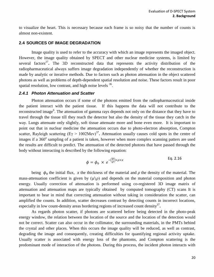
Evaluation of D-SPECT System 2. Background
20
to visualize the heart. This is necessary because each frame is so noisy that the number of counts is
almost non-existent.
2.4 SOURCES OF IMAGE DEGRADATION
Image quality is used to refer to the accuracy with which an image represents the imaged object.
However, the image quality obtained by SPECT and other nuclear medicine systems, is limited by
several factors27
. The 3D reconstructed data that represents the activity distribution of the
radiopharmaceutical always suffers image degradation independently of whether the reconstruction is
made by analytic or iterative methods. Due to factors such as photon attenuation in the object scattered
photons as well as problems of depth-dependent spatial resolution and noise. These factors result in poor
spatial resolution, low contrast, and high noise levels 36
.
2.4.1 Photon Attenuation and Scatter
Photon attenuation occurs if some of the photons emitted from the radiopharmaceutical inside
the patient interact with the patient tissue. If this happens the data will not contribute to the
reconstructed image6. The attenuation of gamma rays depends not only on the distance that they have to
travel through the tissue till they reach the detector but also the density of the tissue they catch in the
way. Lungs attenuate only slightly, soft tissue attenuate more and bone even more. It is important to
point out that in nuclear medicine the attenuation occurs due to photo-electron absorption, Compton
scatter, Rayleigh scattering (Eγ > 1002Mev)37
. Attenuation usually causes cold spots in the centre of
images if a 360o sampling of a patient is taken, however when more complex scanning patters are used
the results are difficult to predict. The attenuation of the detected photons that have passed through the
body without interacting is described by the following equation:
Eq. 2.16
being the initial flux, the thickness of the material and the density of the material. The
mass-attenuation coefficient is given by ( ρ) and depends on the material composition and photon
energy. Usually correction of attenuation is performed using co-registered 3D image matrix of
attenuation and attenuation maps are typically obtained by computed tomography (CT) scans It is
important to bear in mind that correcting attenuation without taking in consideration the scatter, can
amplified the counts. In addition, scatter decreases contrast by detecting counts in incorrect locations,
especially in low count-density areas bordering regions of increased count density37
.
As regards photon scatter, if photons are scattered before being detected in the photo-peak
energy window, the relation between the location of the source and the location of the detection would
not be correct. Scatter can also occur in the collimator, the surrounding materials, in the PMTs behind
the crystal and other places. When this occurs the image quality will be reduced, as well as contrast,
degrading the image and consequently, creating difficulties for quantifying regional activity uptake.
Usually scatter is associated with energy loss of the phantoms, and Compton scattering is the
predominant mode of interaction of the photons. During this process, the incident photon interacts with

Evaluation of D-SPECT System 2. Background
21
an atomic electron and a fraction of its energy is transferred to the electron. At the same time the photon
suffers scatter at an angle ɵ in relation to its original direction. Since scattered photons have less energy
due to suffered iterations, a typical way to reduce scatter is creating an energy window and accept only
counts that fall in that energy window6.
2.4.2 Distance- Dependent Spatial Resolution
The spatial resolution of a camera is another cause of image degradation. The spatial resolution
depends on the distance where the collimator is in relation to the patient and also on the diameter, shape
of the holes and the thickness and length of the septa. The spatial resolution is distance dependent, so
what happens is that as the source gets further away from the camera the full width at a half maximum
(FWHM) gets larger, creating blurred images and bad definition of structures. As a consequence, even
though the number of counts acquired on the camera is correct, the locations of events are spread out
over a large area (more pixels) if the source is located further. Partial-volume effect gets worse when the
source is so far that the pixel will not reflect the right activity in a particular voxel6. The contrast is also
affected, creating difficulties in detecting lesions.
Data obtained by a dynamic scan suffers from blur due to spill-over and partial volume effect. In
dynamic scans, spill over is a bidirectional process that occurs when a percentile of tracer in blood is
found in the tissue and some tracer in tissue is being counted as tracer in blood38
. The choice of ROI to
obtain time-activity curves of dynamic scans is very important and should be chosen so the spillover
could be minimized. Nonetheless, this problem will usually be present, so correction should be applied2.
2.4.3 Image Noise
Image noise occurs due to the random nature of radioactive decay. The noise distribution of
scintillation camera images is in accordance with the Poisson law, meaning the disintegration of an atom
is independently from the disintegration of other atoms of the radiopharmaceutical39
. As a result, to
obtain an image with good quality, the acquisition time should be sufficiently long and the activity of the
radiopharmaceutical high enough40
, because increased counts result in reduced noise41
. These factors
should be optimized in order to avoid the creation of artifacts in the final image. Other factors such as
acquisition time per projection, number of projections, sensitivity of the collimator, detector system, and
matrix size, also influence the noise39
.
SPECT images are more affected by noise than planar images and that is caused by several
factors. SPECT acquisition is done for a relative short time, so the number of counts in each projection
is lower than the counts obtained in planar scans. In addition, noise is amplified if reconstructed with
FBP. This happens because noise in an individual projection is propagated into the 3D matrix.
Reconstructions with iterative algorithms improve the images eliminating some of these factors. For
example, the MLEM algorithm considered the count density as a Poisson function of the radioactivity
distribution and not a single defined value. Nevertheless, as mentioned before, these iterative algorithms
will increase the level of noise as the number of iterations increase. Consequently, noise will be always
present independent of the reconstruction algorithm used, and it will always be a limiting factor of
SPECT images.
Evaluation of D-SPECT System 2. Background
22
2.4.4 Image Truncation
Truncation artifacts are errors that usually occur when portions of the body move out the field of
view (FOV) of some angles. They can also be set up to be intentionally smaller than some portions of
the body. The artefacts are well identified because they are usually bright arcs of activity on the edge of
the patient body if FBP reconstruction is used, and a complex distortion also on the edge if an iterative
algorithm is applied42
. Truncation also occurs during cardiac SPECT acquisitions, again due to the
limited FOV. Artifacts are obtained due to inconsistent data and can be spread onto the heart-wall near
the truncation section43,44
.
2.5 SIMULATION TOOLS
2.5.1 Camera Simulation Tool
To perform the proposed study a camera simulator tool was written in Matlab. Simulation plays
an important role in the field of medical imaging because it helps to evaluate, characterize and optimize
the systems in a simple and realistic way. The tool is used to simulate projection data obtain by gamma
cameras, specifically for D-SPECT camera. The camera simulator tool (or D-SPECT simulator) has
several interfaces for intuitive use. To better understand the model, it will be considered as divided in
two different parts, according to two different interfaces, the main interface (Model_Interface) and the
D-SPECT interface (D_SPECT).
2.5.1.1 Main Interface
The main interface is used to model and save the projections from a simulated D-SPECT (and
also SPECT) acquisition. The main interface is shown in Fig. A in Appendix and on the left side of the
interface, the user can select a camera, that is available on the database, or set up a new one. A source
can also be selected from the existing files on the database, usually a phantom that can be set up.
The source is used in the simulation because it contains details of activity distribution simulating
a real person with the radiopharmaceutical in the blood stream. With the chosen camera and source it is
possible to modulate the projections patterns. There are some options that can be included or excluded
during modulation such as noise, spatial resolution and attenuation, but the scatter is not modelled (there
is no option available). A slice by slice convolution and summing algorithm was applied to model the
depth-dependent resolution. To obtain projections a source matrix is rotated to be parallel to the detector
and numerous small cross kernels are applied to give the correct point spread function at a certain
depth45
.
For attenuation modelling, attenuation maps are needed, including coefficients of linear
attenuation suitable for the energy of gamma emissions from the radionuclide. The simulator is only
modelled for 99m
Tc with emissions at 140keV. The model is voxel based and proceeds on a slice by
slice basis within the same routine as the resolution modelling. The method was derived from46
.
Attenuation projections with resolution modelling were calculated by the program according to the
follow equation:
Eq. 2.17
Evaluation of D-SPECT System 2. Background
23
With xn the activity distribution in a slice, an the linear attenuation coefficient map of the slice v
that is the slice thickness and hn is the incremental blurring kernel associated with that slice45
.
The sensitivity is also modelled and it is used to calculate the number of counts expected from a
scan pattern, scan time, source activity and activity distributions. The factors are taken into account in
the simulation of Poisson noise. The simulator consider that sensitivity depends on the branching ratio
(ratio of alternative products formed in a reaction, being 89% for 140 keV gamma emissions from 99m
Tc), collimator efficiency and effective absorption in the detector used. The noise can then be
modelled selecting a total scanning time and activity in MBq or through the total number of detected
counts, defined by the user. The way the simulator was programmed to calculate the number of counts is
based on the following equation.
Eq. 2.18
X represent the total activity of the source in Bq, T the total scan time, N the number of detector
positions to create a frame. BR is the branching ratio and Aeff is the effective absorption. After
determining the number of counts the Matlab function imnoise is used to generate and add the required
levels of Poisson noise to each projection.
There is also an option Group Angles, to group the angles of the detectors, reducing the scan
time. After calculating the projections, reconstructed data can be obtained. The reconstruction algorithm
used in this model is OS-EM but the simulator tool is slow, and was not used. The simulator was
developed so that the calculated projections were in a format than can be read by the reconstruction
program from Spectrum Dynamic. This program was specially developed to reconstruct D-SPECT
projections obtained clinically by the real D-SPECT scan. The program allows one to select several
parameters, including defining a number of iterations for the reconstructions or defining a filter. Its
interface can be visualized in the appendix Fig B.
2.5.1.2 D-SPECT Interface
If the user selects the option set up camera in the Main Interface, that means that a new camera
can be created and later on, saved (Appendix Fig. A). To set-up a D-SPECT camera it is necessary to
first calculate a scan pattern, and for that a D-SPECT camera and a source should be used and a ROI and
a FOV can be selected. Then a scanning pattern can be calculated and visualized using this interface,
and the scanning pattern will be saved (Matlab structure). That camera can then be used to calculate the
projections using the main interface. Additional information can be set up such as the number of gantry
positions, the total rotational detector positions and the proportion of scan time on ROI (SPR) that is
directly related to the way the scan patterns are calculated. The first two variables should be left as
default if the user wants to create a typical D-SPECT acquisition, using 2 cameras positions over 120
angles. The simulator will create an animation that shows all the detectors rotating from left to right
through 60°, and then the camera rotates 9° to fill sampling gaps and the detectors scan again. In Fig.
2.13 it is possible to visualize the 120 angles positions of the 9 detectors, obtained by the simulator,
showing that they are all rotating in the same direction, being different from the real D-SPECT. The
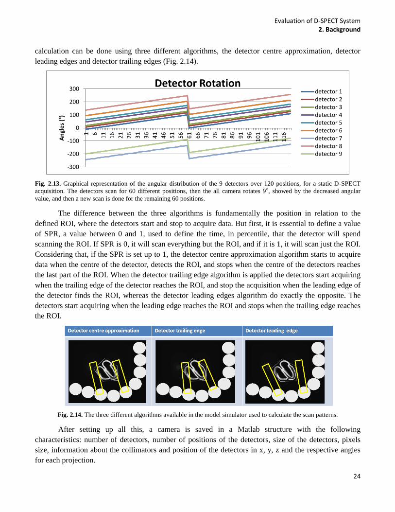
Evaluation of D-SPECT System 2. Background
24
calculation can be done using three different algorithms, the detector centre approximation, detector
leading edges and detector trailing edges (Fig. 2.14).
Fig. 2.13. Graphical representation of the angular distribution of the 9 detectors over 120 positions, for a static D-SPECT
acquisition. The detectors scan for 60 different positions, then the all camera rotates 9o, showed by the decreased angular
value, and then a new scan is done for the remaining 60 positions.
The difference between the three algorithms is fundamentally the position in relation to the
defined ROI, where the detectors start and stop to acquire data. But first, it is essential to define a value
of SPR, a value between 0 and 1, used to define the time, in percentile, that the detector will spend
scanning the ROI. If SPR is 0, it will scan everything but the ROI, and if it is 1, it will scan just the ROI.
Considering that, if the SPR is set up to 1, the detector centre approximation algorithm starts to acquire
data when the centre of the detector, detects the ROI, and stops when the centre of the detectors reaches
the last part of the ROI. When the detector trailing edge algorithm is applied the detectors start acquiring
when the trailing edge of the detector reaches the ROI, and stop the acquisition when the leading edge of
the detector finds the ROI, whereas the detector leading edges algorithm do exactly the opposite. The
detectors start acquiring when the leading edge reaches the ROI and stops when the trailing edge reaches
the ROI.
Fig. 2.14. The three different algorithms available in the model simulator used to calculate the scan patterns.
After setting up all this, a camera is saved in a Matlab structure with the following
characteristics: number of detectors, number of positions of the detectors, size of the detectors, pixels
size, information about the collimators and position of the detectors in x, y, z and the respective angles
for each projection.
-300
-200
-100
0
100
200
300 1
6
11
16
21
26
31
36
41
46
51
56
61
66
71
76
81
86
91
96
10
1
10
6
11
1
11
6
An
gle
s (°
)
Detector Rotation detector 1 detector 2 detector 3 detector 4 detector 5 detector 6 detector 7 detector 8 detector 9
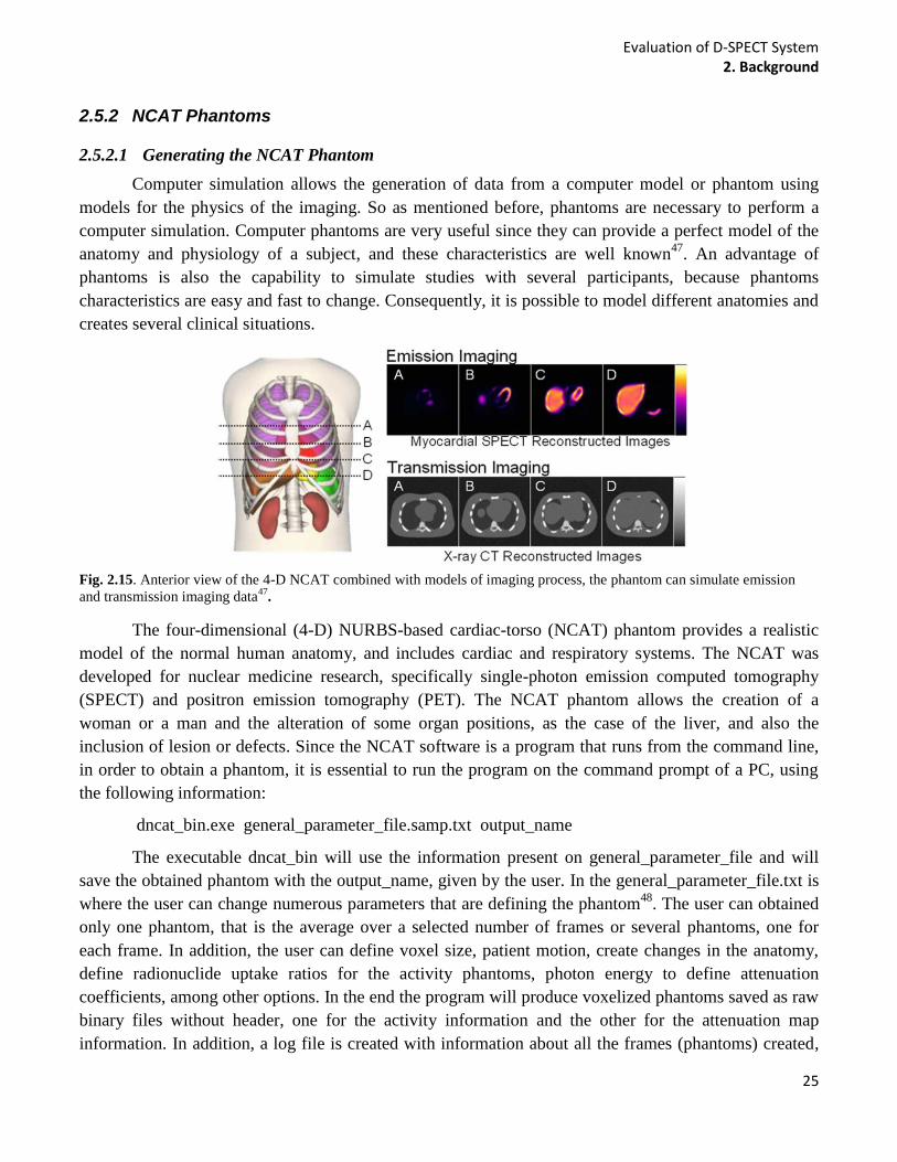
Evaluation of D-SPECT System 2. Background
25
2.5.2 NCAT Phantoms
2.5.2.1 Generating the NCAT Phantom
Computer simulation allows the generation of data from a computer model or phantom using
models for the physics of the imaging. So as mentioned before, phantoms are necessary to perform a
computer simulation. Computer phantoms are very useful since they can provide a perfect model of the
anatomy and physiology of a subject, and these characteristics are well known47
. An advantage of
phantoms is also the capability to simulate studies with several participants, because phantoms
characteristics are easy and fast to change. Consequently, it is possible to model different anatomies and
creates several clinical situations.
Fig. 2.15. Anterior view of the 4-D NCAT combined with models of imaging process, the phantom can simulate emission
and transmission imaging data47
.
The four-dimensional (4-D) NURBS-based cardiac-torso (NCAT) phantom provides a realistic
model of the normal human anatomy, and includes cardiac and respiratory systems. The NCAT was
developed for nuclear medicine research, specifically single-photon emission computed tomography
(SPECT) and positron emission tomography (PET). The NCAT phantom allows the creation of a
woman or a man and the alteration of some organ positions, as the case of the liver, and also the
inclusion of lesion or defects. Since the NCAT software is a program that runs from the command line,
in order to obtain a phantom, it is essential to run the program on the command prompt of a PC, using
the following information:
dncat_bin.exe general_parameter_file.samp.txt output_name
The executable dncat_bin will use the information present on general_parameter_file and will
save the obtained phantom with the output_name, given by the user. In the general_parameter_file.txt is
where the user can change numerous parameters that are defining the phantom48
. The user can obtained
only one phantom, that is the average over a selected number of frames or several phantoms, one for
each frame. In addition, the user can define voxel size, patient motion, create changes in the anatomy,
define radionuclide uptake ratios for the activity phantoms, photon energy to define attenuation
coefficients, among other options. In the end the program will produce voxelized phantoms saved as raw
binary files without header, one for the activity information and the other for the attenuation map
information. In addition, a log file is created with information about all the frames (phantoms) created,

Evaluation of D-SPECT System 2. Background
26
with data about activity in each organ, phase of the cardiac cycle, heart volumes among other
characteristics. There are also other extra files in the program that can be used. For example, it is
possible to generate perfusion defects, obtain heart and respiratory motion vectors or create spherical
lesions in the lungs or liver. These files do not create phantoms with this information, but instead create
files with only the extra information. For example, the program will create voxelized activity or
attenuation phantoms of just the lesion. In order to use the created phantom(s) in the model interface, the
bin files had to be converted to a Matlab structures.
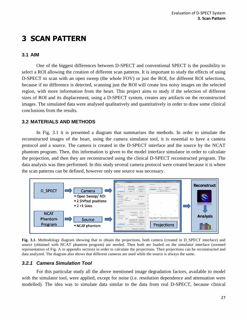
Evaluation of D-SPECT System 3. Scan Pattern
27
3 SCAN PATTERN
3.1 AIM
One of the biggest differences between D-SPECT and conventional SPECT is the possibility to
select a ROI allowing the creation of different scan patterns. It is important to study the effects of using
D-SPECT to scan with an open sweep (the whole FOV) or just the ROI, for different ROI selections,
because if no difference is detected, scanning just the ROI will create less noisy images on the selected
region, with more information from the heart. This project aims to study if the selection of different
sizes of ROI and its displacement, using a D-SPECT system, creates any artifacts on the reconstructed
images. The simulated data were analysed qualitatively and quantitatively in order to draw some clinical
conclusions from the results.
3.2 MATERIALS AND METHODS
In Fig. 3.1 it is presented a diagram that summarises the methods. In order to simulate the
reconstructed images of the heart, using the camera simulator tool, it is essential to have a camera
protocol and a source. The camera is created in the D-SPECT interface and the source by the NCAT
phantom program. Then, this information is given to the model interface simulator in order to calculate
the projection, and then they are reconstructed using the clinical D-SPECT reconstructed program. The
data analysis was then performed. In this study several camera protocol were created because it is where
the scan patterns can be defined, however only one source was necessary.
Fig. 3.1. Methodology diagram showing that to obtain the projections, both camera (created in D_SPECT interface) and
source (obtained with NCAT phantom program) are needed. Then both are loaded on the simulator interface (zoomed
representation of Fig. A in appendix section) in order to calculate the projections. Then projections can be reconstructed and
data analyzed. The diagram also shows that different cameras are used while the source is always the same.
3.2.1 Camera Simulation Tool
For this particular study all the above mentioned image degradation factors, available to model
with the simulator tool, were applied, except for noise (i.e. resolution dependence and attenuation were
modelled). The idea was to simulate data similar to the data from real D-SPECT, because clinical
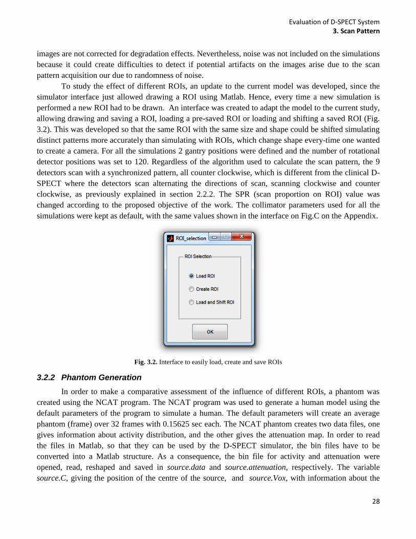
Evaluation of D-SPECT System 3. Scan Pattern
28
images are not corrected for degradation effects. Nevertheless, noise was not included on the simulations
because it could create difficulties to detect if potential artifacts on the images arise due to the scan
pattern acquisition our due to randomness of noise.
To study the effect of different ROIs, an update to the current model was developed, since the
simulator interface just allowed drawing a ROI using Matlab. Hence, every time a new simulation is
performed a new ROI had to be drawn. An interface was created to adapt the model to the current study,
allowing drawing and saving a ROI, loading a pre-saved ROI or loading and shifting a saved ROI (Fig.
3.2). This was developed so that the same ROI with the same size and shape could be shifted simulating
distinct patterns more accurately than simulating with ROIs, which change shape every-time one wanted
to create a camera. For all the simulations 2 gantry positions were defined and the number of rotational
detector positions was set to 120. Regardless of the algorithm used to calculate the scan pattern, the 9
detectors scan with a synchronized pattern, all counter clockwise, which is different from the clinical D-
SPECT where the detectors scan alternating the directions of scan, scanning clockwise and counter
clockwise, as previously explained in section 2.2.2. The SPR (scan proportion on ROI) value was
changed according to the proposed objective of the work. The collimator parameters used for all the
simulations were kept as default, with the same values shown in the interface on Fig.C on the Appendix.
Fig. 3.2. Interface to easily load, create and save ROIs
3.2.2 Phantom Generation
In order to make a comparative assessment of the influence of different ROIs, a phantom was
created using the NCAT program. The NCAT program was used to generate a human model using the
default parameters of the program to simulate a human. The default parameters will create an average
phantom (frame) over 32 frames with 0.15625 sec each. The NCAT phantom creates two data files, one
gives information about activity distribution, and the other gives the attenuation map. In order to read
the files in Matlab, so that they can be used by the D-SPECT simulator, the bin files have to be
converted into a Matlab structure. As a consequence, the bin file for activity and attenuation were
opened, read, reshaped and saved in source.data and source.attenuation, respectively. The variable
source.C, giving the position of the centre of the source, and source.Vox, with information about the
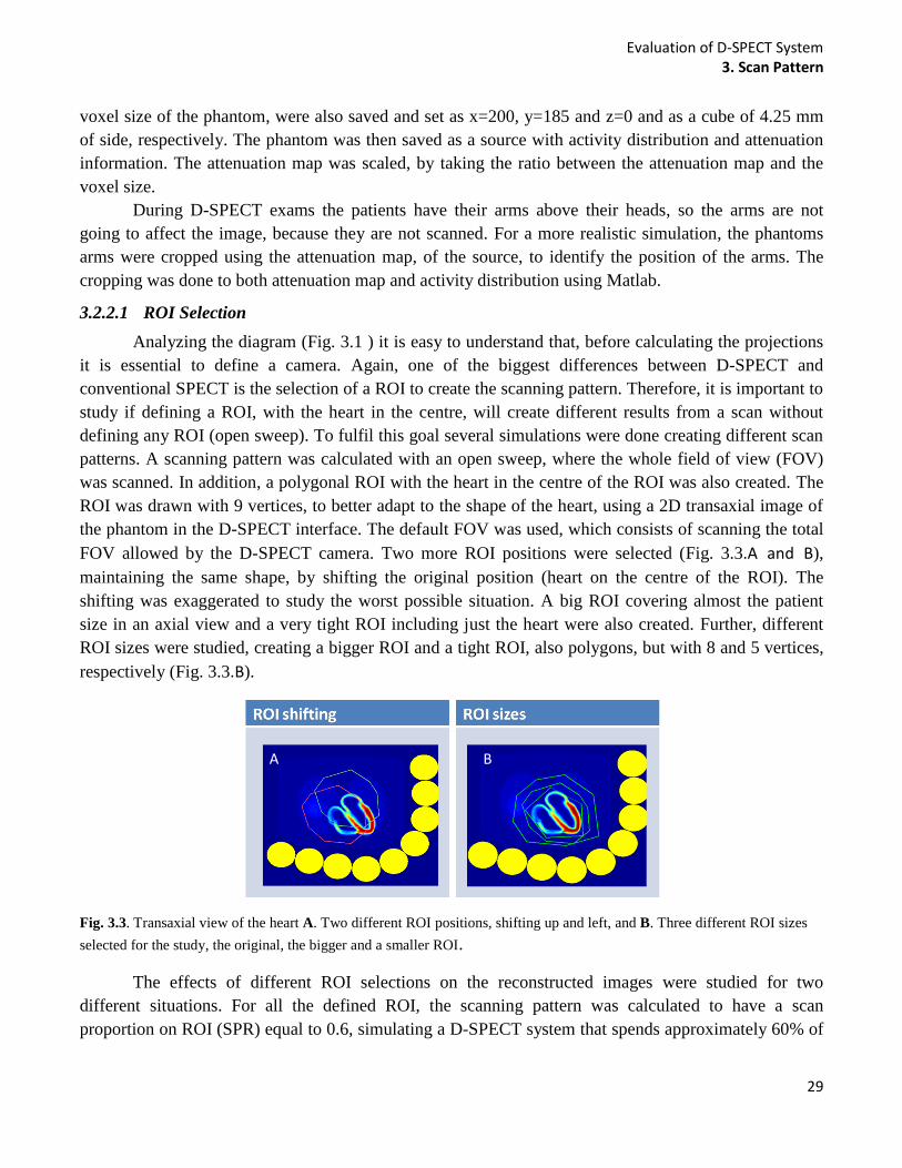
Evaluation of D-SPECT System 3. Scan Pattern
29
voxel size of the phantom, were also saved and set as x=200, y=185 and z=0 and as a cube of 4.25 mm
of side, respectively. The phantom was then saved as a source with activity distribution and attenuation
information. The attenuation map was scaled, by taking the ratio between the attenuation map and the
voxel size.
During D-SPECT exams the patients have their arms above their heads, so the arms are not
going to affect the image, because they are not scanned. For a more realistic simulation, the phantoms
arms were cropped using the attenuation map, of the source, to identify the position of the arms. The
cropping was done to both attenuation map and activity distribution using Matlab.
3.2.2.1 ROI Selection
Analyzing the diagram (Fig. 3.1 ) it is easy to understand that, before calculating the projections
it is essential to define a camera. Again, one of the biggest differences between D-SPECT and
conventional SPECT is the selection of a ROI to create the scanning pattern. Therefore, it is important to
study if defining a ROI, with the heart in the centre, will create different results from a scan without
defining any ROI (open sweep). To fulfil this goal several simulations were done creating different scan
patterns. A scanning pattern was calculated with an open sweep, where the whole field of view (FOV)
was scanned. In addition, a polygonal ROI with the heart in the centre of the ROI was also created. The
ROI was drawn with 9 vertices, to better adapt to the shape of the heart, using a 2D transaxial image of
the phantom in the D-SPECT interface. The default FOV was used, which consists of scanning the total
FOV allowed by the D-SPECT camera. Two more ROI positions were selected (Fig. 3.3.A and B),
maintaining the same shape, by shifting the original position (heart on the centre of the ROI). The
shifting was exaggerated to study the worst possible situation. A big ROI covering almost the patient
size in an axial view and a very tight ROI including just the heart were also created. Further, different
ROI sizes were studied, creating a bigger ROI and a tight ROI, also polygons, but with 8 and 5 vertices,
respectively (Fig. 3.3.B).
Fig. 3.3. Transaxial view of the heart A. Two different ROI positions, shifting up and left, and B. Three different ROI sizes
selected for the study, the original, the bigger and a smaller ROI.
The effects of different ROI selections on the reconstructed images were studied for two
different situations. For all the defined ROI, the scanning pattern was calculated to have a scan
proportion on ROI (SPR) equal to 0.6, simulating a D-SPECT system that spends approximately 60% of
A B
Evaluation of D-SPECT System 3. Scan Pattern
30
the scanning time inside the ROI and the rest outside the FOV. Scanning patterns were also calculated
with SPR equal to 1, to simulate a FOV equal to the ROI, where the detectors will scan just the ROI.
The SPR equal to 0.6 is a good approximation to what it is obtained clinically by D-SPECT when
combined with the employment of detector leading edges algorithm to calculate the projections for all
the scan patterns. An extra simulation was done calculating the projection with the detector trailing edge
algorithm, for the tight ROI, in order to create an even smaller ROI.
Each scan pattern was calculated for each ROI selection and for each SPR value, creating a total
of 12 scanning patterns, each saved as a structure called camera, with information about the detector
motion and acquisition angles. To calculate the scanning pattern for all the 12 cameras using only one
source (the created phantom) without having to do it one at a time a script was created. The script called
the Matlab structure camFile, where all the 12 cameras were saved and then calculates the projections
successively for each of the cameras used, with always the same source.
3.2.2.2 Data Reconstruction
After obtaining the projections, the data were reconstructed using the Spectrum Dynamics
program, as used clinically to reconstruct patient data. Clinically, the data are reconstructed using 3
initial iterations and 4 further iterations after fitting the reconstruction to a model of the heart. However,
for the reconstructions in this study, 7 iterations were used and no model fitting was applied. A filter was
used between iterations, a convolution between two triangular filters to smooth the image, but a post-
reconstruction-filter was not used. After the 7 iterations were finished, it is possible to align the heart so
that it appears on the right views of the vertical long axis (VLA), horizontal long axis (HLA) and short
axis (SA). An ini file was created by the reconstruction program with information about heart
orientations. Additionally, the output data with the reconstructed images was given by an est file, for
each iteration, individually. Thus, the ini file correspondent to reconstruction with 7 iterations was
selected, in order to be visualized by different analysis programs.
3.2.2.3 Image Analysis Tools
For data interpretation and better diagnosis using nuclear cardiac imaging, it is very important to
analyse the images qualitatively and quantitatively. The computer analysis is important to evaluate the
images because it is independent of the observer inconsistency.
The est file data from the 7 iteration reconstructions was opened in Amide a medical imaging
data examiner (AMIDE) for image analysis and visualization of the reconstructed data from transaxial,
sagittal and coronal views. Some inputs are needed to correctly display the images. Despite the size of
the source being 128x128x128, the detectors are smaller, so after the reconstruction the images have a
70x60x81 size and the voxel size is 4.92 mm. An image is generated with these parameters, but in order
to visualize it correctly a ROI should be created and the maximal pixel value calculated. Knowing that
specific value and using it as the absolute maximum threshold for the image, the reconstructed image
can be visualized correctly. Amide allows the visualization of all the slices in each of the different
views, the number of counts along a line can also be calculated and visualized in a graphic for different
images at the same time. Images can also be summed or subtracted has a better comparison between
different data.

Evaluation of D-SPECT System 3. Scan Pattern
31
The est file was also converted to a dicom file (dcm) in order to be opened in the quantitative
perfusion SPECT program (QPS), creating the bullseye plot. QPS is an interactive application for an
automatic quantification involving segmentation, analysis and display of myocardial perfusion SPECT.
This program is the one used clinically to assess results from rest and stress acquisition protocols.
After analysing visually all the resulting images, it was decided to analyze qualitatively 4 of the
12 simulations scan patterns (Fig. 3.4). The values for each segment were plotted (bar plots), for the
Open Sweep, Clinical ROI (tight ROI for SPR=0.6), ROI only (tight ROI for SPR=1) and small ROI
(tight ROI for SPR=1 and detector trailing edge algorithm). Instead of analysing the bullseye with the 20
segments, only 14 (from 7 to 20) were used. The outer ring of the polar plot was not considered since it
does not contain much information about the activity, and it is almost the same for all the data. The
values for each segment for the open sweep, ROI only and small ROI were plotted against the clinical
type of scan and some statistical measures were obtained following plotting the linear regression of the
scatter plot data. The square of the coefficient of correlation (R2) was obtained, to measure the
correlation between segment values and the standard error of estimation (SEE) that gives information
about the spread of the data, was also calculated.
Fig. 3.4. Scheme of the four different scan patterns created. For Open sweep the whole FOV is scanned, the Clinical represent the scan pattern performed by D-SPECT clinically, where a ROI is defined and the detectors spend around 60% of the time scanning inside the ROI and the remaining time on the rest of the FOV. ROI only, only the ROI is scanned using detector leading edge algorithm to calculate the projections while for the small ROI the detector trailing edge was the one applied.
All four images were analysed in Matlab. A 3D mask, based on intensity, was built to select the
left ventricle of the myocardium that is usually the part of the heart that is analysed for cardiac
diagnostics, because it is the heart's main pumping chamber, pushing oxygen-rich blood to the entire
body. The mask was applied to the reconstructed image obtained with the open sweep scan patterns and
applied for the rest of the data. Nonetheless, applying only a threshold value to pick the LV is difficult
because some parts of the spine and other body parts have similar intensity values. Therefore the
CC=bwconncomp Matlab function was used to select distinct clusters that were found in the 3D image
after applying the mask. Each one was labelled, so that only the label of the heart could be chosen. After
selecting the LV for each reconstructed image, the mean activity values were saved.

Evaluation of D-SPECT System 3. Scan Pattern
32
3.3 RESULTS AND DISCUSSION
In Fig. 3.5 the reconstructed images acquired with two different cameras are shown, one with a
selected ROI with the heart on the centre and the other where the ROI had suffered a shift, moving the
left ventricle out of the region of interest (shifted up). Both images sets are shown in three different
views available from the program AMIDE. Independently of the view, there is no evident difference
between the two reconstructed images. Similar results were found for the other shifted ROI and the
bigger and tight ROI (Fig. 3.3 B). Even though the ROI have changed considerably between simulations
the projections will always acquire the whole heart. So, since noise is not being modelled the
reconstructed image will always find the best estimate of the distribution, justifying the good
reconstructions for all the simulations.
Fig. 3.5. Clinical transverse, coronal and sagittal views of the LV of the heart for two different scan patterns, taken from
AMIDE. The initial ROI represents the ROI where the heart is on the centre of the region and the size of it corresponds to the
first simulation.
In Fig. 3.6 the reconstructed images on an axial slice obtained with open sweep scan, clinical
scan, ROI only and small ROI are shown. The axial slice was selected so that the middle of the heart
could be displayed. All the 4 images were scaled to the maximal value obtained on the plotted using the
clinical scan pattern. The images were plotted in Matlab and rotated to be displayed in the same way as
the simulator interface. Analyzing in more detail one axial slice of each 4 simulations, there is not much
difference found between all of them (Fig. 3.6). Nonetheless, one can see some artifacts on the last two
images due to the truncation affect, especially for the small ROI data. For this last reconstructed image,
values of high activity were found around the heart, as a consequence of the truncation.

Evaluation of D-SPECT System 3. Scan Pattern
33
Fig. 3.6. Reconstructed images for four different scan patterns. The left ventricle of the myocardium seems to become thinner from data from left to right. Right ventricle and atria are not visible for the small ROI scan patterns, and there are artefacts around the heart.
What happens is that photons from other parts of the body, for example the liver, will also reach
the detector, but it cannot see where the information comes from, since it is not acquiring the complete
amount of data. In practice this is not a problem because usually the image is cropped and this effect
would not be noticed, because the important data to reconstruct correctly is in the heart. Beyond that, the
right ventricle and atrium of the heart were visible for all the simulations apart from the small ROI. The
left ventricle of the myocardium also seems to get thinner from left to right reconstructed images on Fig.
3.6, being more evident on the small ROI data, where the LV is even more flattened, when compared
with the other results. The similarities could be justified taking into account that the only difference
between the acquisition performed with open sweep, clinical and ROI only is the time spent on the ROI.
Again, the similarities arise because since no noise is being modelled, the reconstruction will always
find the best estimate of the distribution. It is important to bear in mind that the detector leading edge
algorithm will create a scanning pattern that starts acquiring before the detector start seeing the ROI, so
it will also scan a considerable area outside the ROI (check Fig. 2.14). This factor also helps justify the
similarities between all the results, since all of the data, except the small ROI, were scanned with
detector leading edge algorithm.
Fig. 3.7. Bullseye plots obtained from QPS for both clinical open sweep and small ROI. Each segment represented has a
value between 1 and 100, given a scale of intensity on that segment.

Evaluation of D-SPECT System 3. Scan Pattern
34
As previously explained quantitative analysis was performed using QPS. In Fig. 3.7 two bullseye
representations are displayed, one for open sweep scan and other for small ROI. The correspondent
value of activity for all the 20 segments are also displayed on the images. To better understand the
results obtained by the bullseye plot, the QPS images showing the short axis of the heart can be assessed
in more detail on Fig. 3.8. Three slices of the short axis view of the heart were obtained and displayed
for open sweep scan, by the QPS program. Similar results were obtained for clinical and ROI scans (not
shown), nevertheless, the program was not able to display the 3 different slices for small ROI images.
Fig. 3.8. Three slices of the short axis of the heart view for both open sweep and small ROI. The two extreme slices of short
axis were not represented when the projections were calculated with small ROI.
Fig. 3.9. Plot of 14 inner rings segment values for open sweep and small ROI scan compared with the values for each
segment of the clinical scan. Respective R2 values are plotted.
Qualitative analysis usually does not give sufficient information to make consistent conclusions.
Based on the segment values obtain by the bullseye plot on Fig. 3.7 and the values obtained for the same
segments with the clinical scan and the ROI only, the graph on Fig. 3.9 was created. The outer ring
values of the bullseye plots were not considered, so from segment value 7 to 20 (check Fig. 2.8), the
values of each segment for open sweep data and small ROI were plotted on the vertical axis, against
R² = 0,9852
R² = 0,9321
50
55
60
65
70
75
80
85
90
95
100
50 60 70 80 90 100
Segm
ent
valu
e
Segment value (Clinical Scan)
Open Sweep smallROI
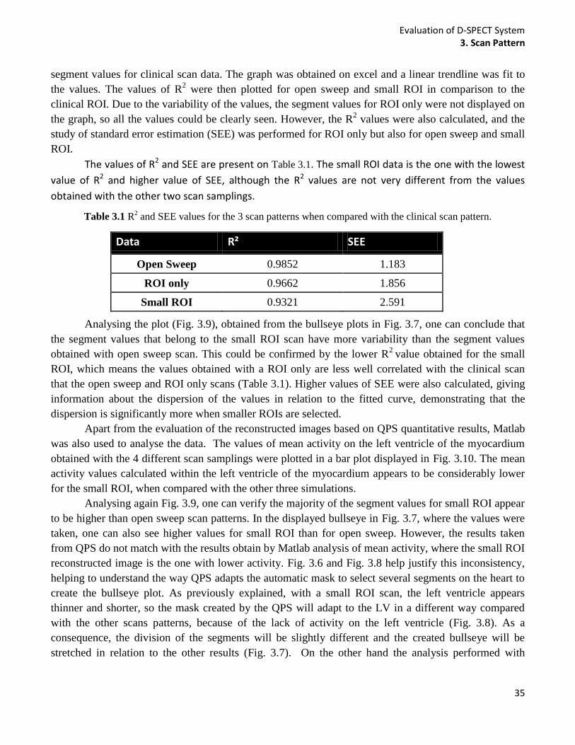
Evaluation of D-SPECT System 3. Scan Pattern
35
segment values for clinical scan data. The graph was obtained on excel and a linear trendline was fit to
the values. The values of R2 were then plotted for open sweep and small ROI in comparison to the
clinical ROI. Due to the variability of the values, the segment values for ROI only were not displayed on
the graph, so all the values could be clearly seen. However, the R2 values were also calculated, and the
study of standard error estimation (SEE) was performed for ROI only but also for open sweep and small
ROI.
The values of R2 and SEE are present on Table 3.1. The small ROI data is the one with the lowest
value of R2 and higher value of SEE, although the R2 values are not very different from the values
obtained with the other two scan samplings.
Table 3.1 R2 and SEE values for the 3 scan patterns when compared with the clinical scan pattern.
Data R² SEE
Open Sweep 0.9852 1.183
ROI only 0.9662 1.856
Small ROI 0.9321 2.591
Analysing the plot (Fig. 3.9), obtained from the bullseye plots in Fig. 3.7, one can conclude that
the segment values that belong to the small ROI scan have more variability than the segment values
obtained with open sweep scan. This could be confirmed by the lower R2
value obtained for the small
ROI, which means the values obtained with a ROI only are less well correlated with the clinical scan
that the open sweep and ROI only scans (Table 3.1). Higher values of SEE were also calculated, giving
information about the dispersion of the values in relation to the fitted curve, demonstrating that the
dispersion is significantly more when smaller ROIs are selected.
Apart from the evaluation of the reconstructed images based on QPS quantitative results, Matlab
was also used to analyse the data. The values of mean activity on the left ventricle of the myocardium
obtained with the 4 different scan samplings were plotted in a bar plot displayed in Fig. 3.10. The mean
activity values calculated within the left ventricle of the myocardium appears to be considerably lower
for the small ROI, when compared with the other three simulations.
Analysing again Fig. 3.9, one can verify the majority of the segment values for small ROI appear
to be higher than open sweep scan patterns. In the displayed bullseye in Fig. 3.7, where the values were
taken, one can also see higher values for small ROI than for open sweep. However, the results taken
from QPS do not match with the results obtain by Matlab analysis of mean activity, where the small ROI
reconstructed image is the one with lower activity. Fig. 3.6 and Fig. 3.8 help justify this inconsistency,
helping to understand the way QPS adapts the automatic mask to select several segments on the heart to
create the bullseye plot. As previously explained, with a small ROI scan, the left ventricle appears
thinner and shorter, so the mask created by the QPS will adapt to the LV in a different way compared
with the other scans patterns, because of the lack of activity on the left ventricle (Fig. 3.8). As a
consequence, the division of the segments will be slightly different and the created bullseye will be
stretched in relation to the other results (Fig. 3.7). On the other hand the analysis performed with

Evaluation of D-SPECT System 3. Scan Pattern
36
Matlab was made so that the same mask could be applied for all the 4 results, showing lower activity
values on small ROI data essentially due to the flattened affect.
Fig. 3.10. Mean activity in the left ventricle of the myocardium selected by a 3D mask based on intensity, for all the four
scan patterns (Open sweep, clinical, ROI only, small ROI).
It is should also be noted that analyzing Fig. 3.5 or Fig. 3.6 and comparing with Fig. 3.8, it is
evident that the resolution for the first images are very poor. The phantoms have a size of 128x128x128,
however during the reconstruction of projections the size is changed. The reconstruction is performed
considering large pixels sizes in order to accelerate the process (that is why it takes less than one minute
to reconstruct a frame). Consequently the images are pour in resolution. However, the reconstructions
performed by D-SPECT reconstructed were developed so that could be open on QPS, and then the
program smoothes the images, improving the resolution.
3.4 CONCLUSION
This study allows the evaluation of the D-SPECT system in terms of effects of different scan
patterns and the importance of selecting an ROI. If only the ROI is scanned, a scan with the same
acquisition time can detect more information from the ROI, compared with scanning the whole FOV, or
spending more time on the ROI, but still scanning the FOV. This will improve sensitivity. No significant
differences were found between distinct ROI selections (shifted and different sizes) except when the
ROI is too small.
Clinically, the ROI only acquisition could be used instead of the current clinical scan pattern,
provided that the ROI is not too small. The clinical scan and the ROI only showed some differences in
terms of segment values, but the R2 and SEE values seem coherent, since they are not very high or very
low respectively. When the acquisition focused too much on the ROI, the heart suffered a flattened
affect and also more variability on the myocardium was observed.
Even though the effect of different scan patterns could be studied without any other factors
interfering, more realistic studies should be performed including Poisson noise, because clinically is
impossible to eliminate the noisy data. This should be checked to understand if the same conclusion can
be drawn or some validations could be performed using a physical phantom in the real D-SPECT
system.
1010
1050
1090
1130
Open Sweep Clinical ROIonly SmallROI
Mea
n a
ctiv
ity
in t
he
LV Scan Pattern
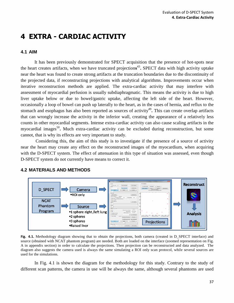
Evaluation of D-SPECT System 4. Extra-Cardiac Activity
37
4 EXTRA - CARDIAC ACTIVITY
4.1 AIM
It has been previously demonstrated for SPECT acquisition that the presence of hot-spots near
the heart creates artifacts, when we have truncated projections43
. SPECT data with high activity uptake
near the heart was found to create strong artifacts at the truncation boundaries due to the discontinuity of
the projected data, if reconstructing projections with analytical algorithms. Improvements occur when
iterative reconstruction methods are applied. The extra-cardiac activity that may interfere with
assessment of myocardial perfusion is usually subdiaphragmatic. This means the activity is due to high
liver uptake below or due to bowel/gastric uptake, affecting the left side of the heart. However,
occasionally a loop of bowel can push up laterally to the heart, as in the cases of hernia, and reflux to the
stomach and esophagus has also been reported as sources of activity49
. This can create overlap artifacts
that can wrongly increase the activity in the inferior wall, creating the appearance of a relatively less
counts in other myocardial segments. Intense extra-cardiac activity can also cause scaling artifacts in the
myocardial images50
. Much extra-cardiac activity can be excluded during reconstruction, but some
cannot, that is why its effects are very important to study.
Considering this, the aim of this study is to investigate if the presence of a source of activity
near the heart may create any effect on the reconstructed images of the myocardium, when acquiring
with the D-SPECT system. The effect of attenuation in this type of situation was assessed, even though
D-SPECT system do not currently have means to correct it.
4.2 MATERIALS AND METHODS
Fig. 4.1. Methodology diagram showing that to obtain the projections, both camera (created in D_SPECT interface) and
source (obtained with NCAT phantom program) are needed. Both are loaded on the interface (zoomed representation on Fig.
A in appendix section) in order to calculate the projections. Then projection can be reconstructed and data analyzed. The
diagram also suggests the camera used is always the same simulating a ROI only scan protocol, while several sources are
used for the simulations.
In Fig. 4.1 is shown the diagram for the methodology for this study. Contrary to the study of
different scan patterns, the camera in use will be always the same, although several phantoms are used
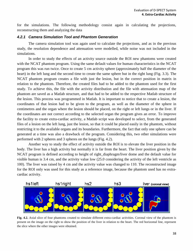
Evaluation of D-SPECT System 4. Extra-Cardiac Activity
38
for the simulations. The following methodology consist again in calculating the projections,
reconstructing them and analyzing the data
4.2.1 Camera Simulation Tool and Phantom Generation
The camera simulation tool was again used to calculate the projections, and as in the previous
study, the resolution dependence and attenuation were modelled, while noise was not included in the
simulations.
In order to study the effects of an activity source outside the ROI new phantoms were created
with the NCAT phantom program. Using the same default values for human characteristics in the NCAT
program this was run twice. Once to create 5 cm activity sphere (approximately half the diameter of the
heart) in the left lung and the second time to create the same sphere but in the right lung (Fig. 3.3). The
NCAT phantom program creates a file with just the lesion, but in the correct position in matrix in
relation to the phantom. Therefore, the created files had to be added to the phantom used for the first
study. To achieve this, the file with the activity distribution and the file with attenuation map of the
phantom are saved as a Matlab structure, and that had to be added to the respective Matlab structure of
the lesion. This process was programmed in Matlab. It is important to notice that to create a lesion, the
coordinates of that lesion had to be given to the program, as well as the diameter of the sphere in
centimetres and the organ where the lesion should be placed, on the right or left lungs or in the liver. If
the coordinates are not correct according to the selected organ the program gives an error. To improve
the facility to create extra-cardiac activity, a Matlab script was developed to select, from the generated
files of a lesion on the left lung, just the lesion, so that it could be placed easily in the phantom, without
restricting it to the available organs and its boundaries. Furthermore, the fact that only one sphere can be
generated at a time was also a drawback of the program. Considering this, two other simulations were
performed with 2 spheres and 3 spheres on the lungs (Fig. 4.2).
Another way to study the effect of activity outside the ROI is to elevate the liver position in the
body. The liver has a high activity but normally it is far from the heart. The liver position given by the
NCAT program is defined according to height of right_diaphragm/liver dome and the default value for
visible human is 3.4 cm, and the activity value low (25.0 considering the activity of the left ventricle as
100). The liver was raised by 4 cm and the activity value was changed to 110. The reconstructed image
for the ROI only was used for this study as a reference image, because the phantom used has no extra-
cardiac activity.
Fig. 4.2. Axial slice of four phantoms created to simulate different extra-cardiac activities. Coronal view of the phantom is
present on the image on the right to show the position of the liver in relation to the heart. The red horizontal line, represent
the slice where the other images were obtained.
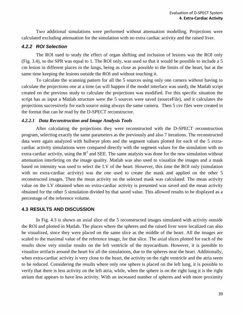
Evaluation of D-SPECT System 4. Extra-Cardiac Activity
39
Two additional simulations were performed without attenuation modelling. Projections were
calculated excluding attenuation for the simulation with no extra cardiac activity and the raised liver.
4.2.2 ROI Selection
The ROI used to study the effect of organ shifting and inclusion of lesions was the ROI only
(Fig. 3.4), so the SPR was equal to 1. The ROI only, was used so that it would be possible to include a 5
cm lesion in different places in the lungs, being as close as possible to the limits of the heart, but at the
same time keeping the lesions outside the ROI and without touching it.
To calculate the scanning pattern for all the 5 sources using only one camera without having to
calculate the projections one at a time (as will happen if the model interface was used), the Matlab script
created on the previous study to calculate the projections was modified. For this specific situation the
script has as input a Matlab structure were the 5 sources were saved (sourceFile), and it calculates the
projections successively for each source using always the same camera. Then 5 csv files were created in
the format that can be read by the D-SPECT reconstructor.
4.2.2.1 Data Reconstruction and Image Analysis Tools
After calculating the projections they were reconstructed with the D-SPECT reconstruction
program, selecting exactly the same parameters as the previously and also 7 iterations. The reconstructed
data were again analyzed with bullseye plots and the segment values plotted for each of the 5 extra-
cardiac activity simulations were compared directly with the segment values for the simulation with no
extra-cardiac activity, using the R2 and SEE. The same analysis was done for the new simulation without
attenuation interfering on the image quality. Matlab was also used to visualize the images and a mask
based on intensity was used to select the LV of the heart. However, this time the ROI only (simulation
with no extra-cardiac activity) was the one used to create the mask and applied on the other 5
reconstructed images. Then the mean activity on the selected mask was calculated. The mean activity
value on the LV obtained when no extra-cardiac activity is presented was saved and the mean activity
obtained for the other 5 simulation divided by that saved value. This allowed results to be displayed as a
percentage of the reference volume.
4.3 RESULTS AND DISCUSSION
In Fig. 4.3 is shown an axial slice of the 5 reconstructed images simulated with activity outside
the ROI and plotted in Matlab. The places where the spheres and the raised liver were localized can also
be visualized, since they were placed on the same slice as the middle of the heart. All the images are
scaled to the maximal value of the reference image, for that slice. The axial slices plotted for each of the
results show very similar results on the left ventricle of the myocardium. However, it is possible to
visualize artifacts around the heart for all the simulations, due to the spheres near the heart. Additionally,
when extra-cardiac activity is very close to the heart, the activity on the right ventricle and the atria seem
to be reduced. Considering the results where only one sphere is placed on the left lung, it is possible to
verify that there is less activity on the left atria, while, when the sphere is on the right lung it is the right
atrium that appears to have less activity. With an increased number of spheres and with more proximity
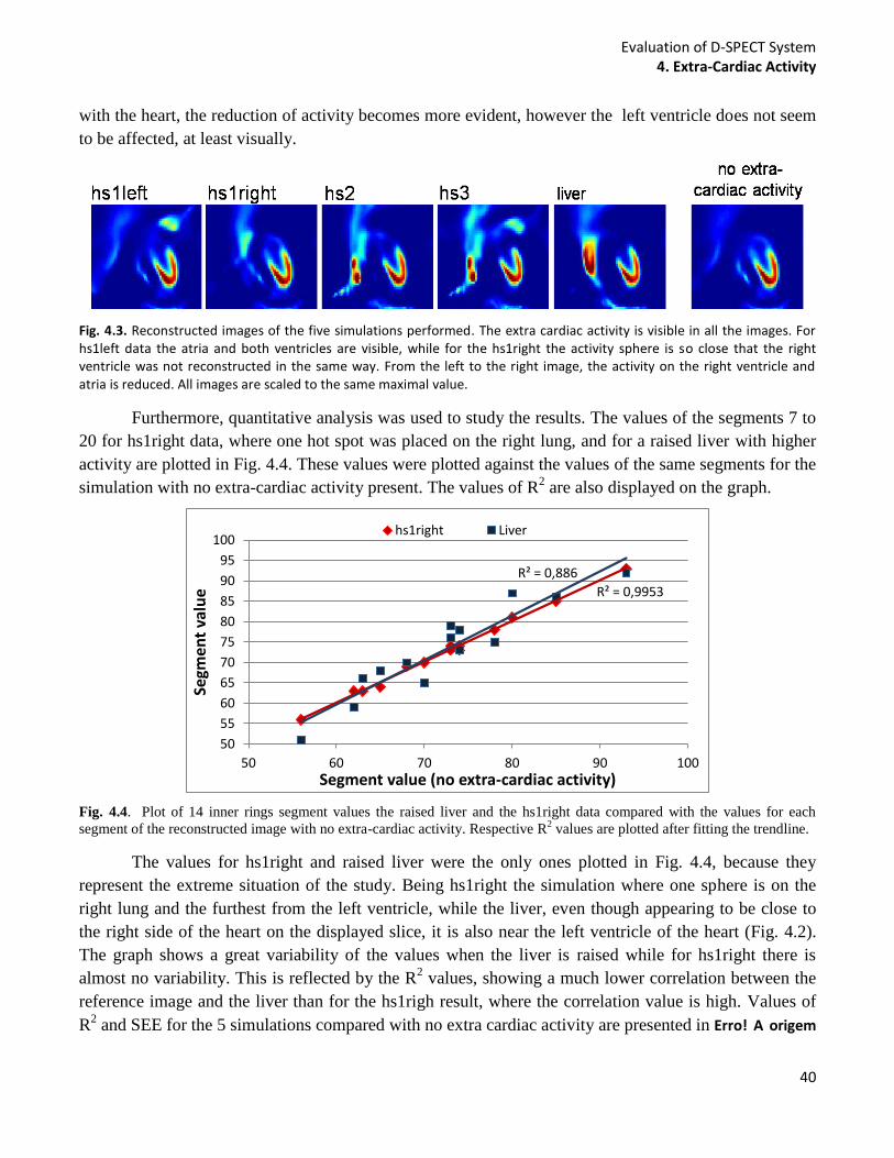
Evaluation of D-SPECT System 4. Extra-Cardiac Activity
40
with the heart, the reduction of activity becomes more evident, however the left ventricle does not seem
to be affected, at least visually.
Fig. 4.3. Reconstructed images of the five simulations performed. The extra cardiac activity is visible in all the images. For hs1left data the atria and both ventricles are visible, while for the hs1right the activity sphere is so close that the right ventricle was not reconstructed in the same way. From the left to the right image, the activity on the right ventricle and atria is reduced. All images are scaled to the same maximal value.
Furthermore, quantitative analysis was used to study the results. The values of the segments 7 to
20 for hs1right data, where one hot spot was placed on the right lung, and for a raised liver with higher
activity are plotted in Fig. 4.4. These values were plotted against the values of the same segments for the
simulation with no extra-cardiac activity present. The values of R2 are also displayed on the graph.
Fig. 4.4. Plot of 14 inner rings segment values the raised liver and the hs1right data compared with the values for each
segment of the reconstructed image with no extra-cardiac activity. Respective R2 values are plotted after fitting the trendline.
The values for hs1right and raised liver were the only ones plotted in Fig. 4.4, because they
represent the extreme situation of the study. Being hs1right the simulation where one sphere is on the
right lung and the furthest from the left ventricle, while the liver, even though appearing to be close to
the right side of the heart on the displayed slice, it is also near the left ventricle of the heart (Fig. 4.2).
The graph shows a great variability of the values when the liver is raised while for hs1right there is
almost no variability. This is reflected by the R2 values, showing a much lower correlation between the
reference image and the liver than for the hs1righ result, where the correlation value is high. Values of
R2 and SEE for the 5 simulations compared with no extra cardiac activity are presented in Erro! A origem
R² = 0,9953
R² = 0,886
50
55
60
65
70
75
80
85
90
95
100
50 60 70 80 90 100
Segm
ent
valu
e
Segment value (no extra-cardiac activity)
hs1right Liver
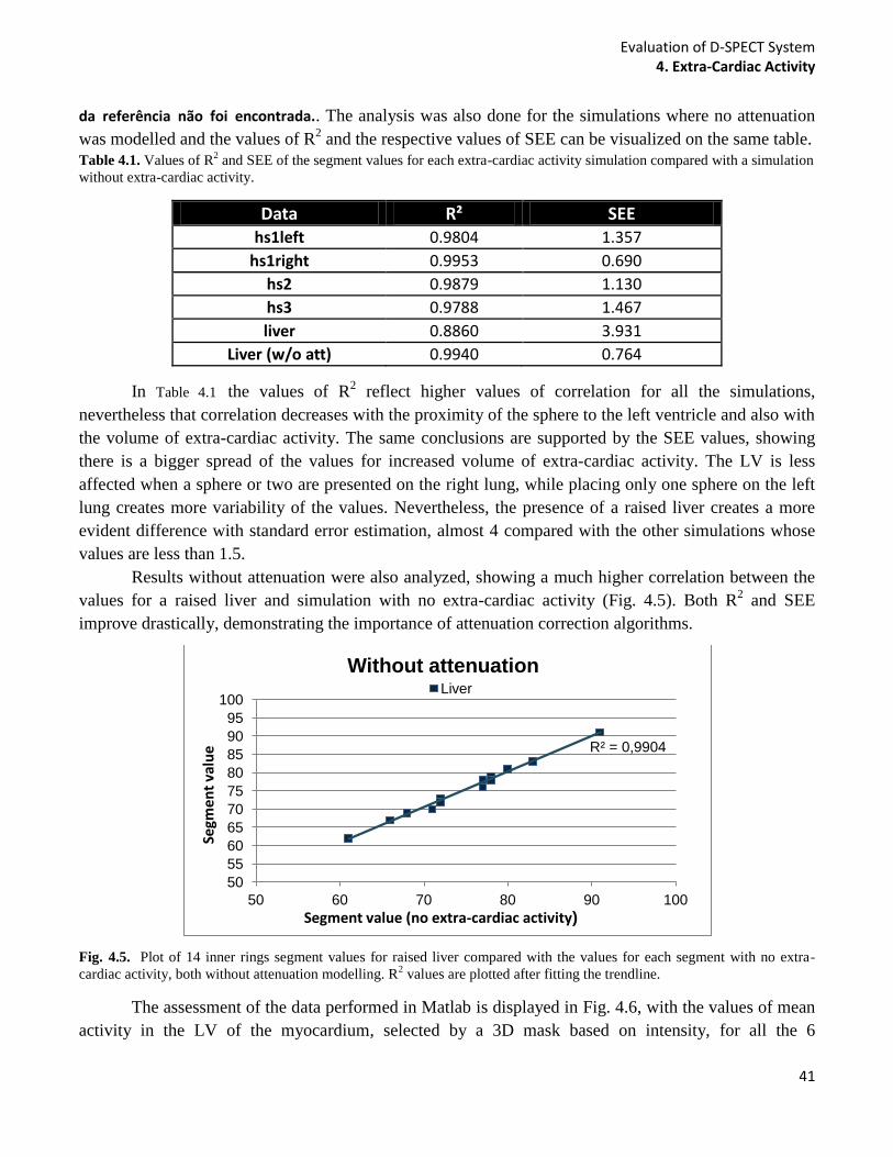
Evaluation of D-SPECT System 4. Extra-Cardiac Activity
41
da referência não foi encontrada.. The analysis was also done for the simulations where no attenuation
was modelled and the values of R2 and the respective values of SEE can be visualized on the same table.
Table 4.1. Values of R2 and SEE of the segment values for each extra-cardiac activity simulation compared with a simulation
without extra-cardiac activity.
Data R² SEE hs1left 0.9804 1.357
hs1right 0.9953 0.690
hs2 0.9879 1.130
hs3 0.9788 1.467
liver 0.8860 3.931
Liver (w/o att) 0.9940 0.764
In Table 4.1 the values of R2 reflect higher values of correlation for all the simulations,
nevertheless that correlation decreases with the proximity of the sphere to the left ventricle and also with
the volume of extra-cardiac activity. The same conclusions are supported by the SEE values, showing
there is a bigger spread of the values for increased volume of extra-cardiac activity. The LV is less
affected when a sphere or two are presented on the right lung, while placing only one sphere on the left
lung creates more variability of the values. Nevertheless, the presence of a raised liver creates a more
evident difference with standard error estimation, almost 4 compared with the other simulations whose
values are less than 1.5.
Results without attenuation were also analyzed, showing a much higher correlation between the
values for a raised liver and simulation with no extra-cardiac activity (Fig. 4.5). Both R2 and SEE
improve drastically, demonstrating the importance of attenuation correction algorithms.
Fig. 4.5. Plot of 14 inner rings segment values for raised liver compared with the values for each segment with no extra-
cardiac activity, both without attenuation modelling. R2 values are plotted after fitting the trendline.
The assessment of the data performed in Matlab is displayed in Fig. 4.6, with the values of mean
activity in the LV of the myocardium, selected by a 3D mask based on intensity, for all the 6
R² = 0,9904
50
55
60
65
70
75
80
85
90
95
100
50 60 70 80 90 100
Segm
en
t va
lue
Segment value (no extra-cardiac activity)
Without attenuation Liver
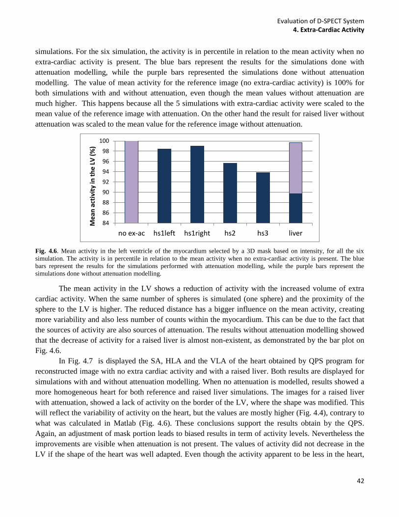
Evaluation of D-SPECT System 4. Extra-Cardiac Activity
42
simulations. For the six simulation, the activity is in percentile in relation to the mean activity when no
extra-cardiac activity is present. The blue bars represent the results for the simulations done with
attenuation modelling, while the purple bars represented the simulations done without attenuation
modelling. The value of mean activity for the reference image (no extra-cardiac activity) is 100% for
both simulations with and without attenuation, even though the mean values without attenuation are
much higher. This happens because all the 5 simulations with extra-cardiac activity were scaled to the
mean value of the reference image with attenuation. On the other hand the result for raised liver without
attenuation was scaled to the mean value for the reference image without attenuation.
Fig. 4.6. Mean activity in the left ventricle of the myocardium selected by a 3D mask based on intensity, for all the six
simulation. The activity is in percentile in relation to the mean activity when no extra-cardiac activity is present. The blue
bars represent the results for the simulations performed with attenuation modelling, while the purple bars represent the
simulations done without attenuation modelling.
The mean activity in the LV shows a reduction of activity with the increased volume of extra
cardiac activity. When the same number of spheres is simulated (one sphere) and the proximity of the
sphere to the LV is higher. The reduced distance has a bigger influence on the mean activity, creating
more variability and also less number of counts within the myocardium. This can be due to the fact that
the sources of activity are also sources of attenuation. The results without attenuation modelling showed
that the decrease of activity for a raised liver is almost non-existent, as demonstrated by the bar plot on
Fig. 4.6.
In Fig. 4.7 is displayed the SA, HLA and the VLA of the heart obtained by QPS program for
reconstructed image with no extra cardiac activity and with a raised liver. Both results are displayed for
simulations with and without attenuation modelling. When no attenuation is modelled, results showed a
more homogeneous heart for both reference and raised liver simulations. The images for a raised liver
with attenuation, showed a lack of activity on the border of the LV, where the shape was modified. This
will reflect the variability of activity on the heart, but the values are mostly higher (Fig. 4.4), contrary to
what was calculated in Matlab (Fig. 4.6). These conclusions support the results obtain by the QPS.
Again, an adjustment of mask portion leads to biased results in term of activity levels. Nevertheless the
improvements are visible when attenuation is not present. The values of activity did not decrease in the
LV if the shape of the heart was well adapted. Even though the activity apparent to be less in the heart,
84
86
88
90
92
94
96
98
100
no ex-ac hs1left hs1right hs2 hs3 liver
Me
an a
ctiv
ity
in t
he
LV (
%)
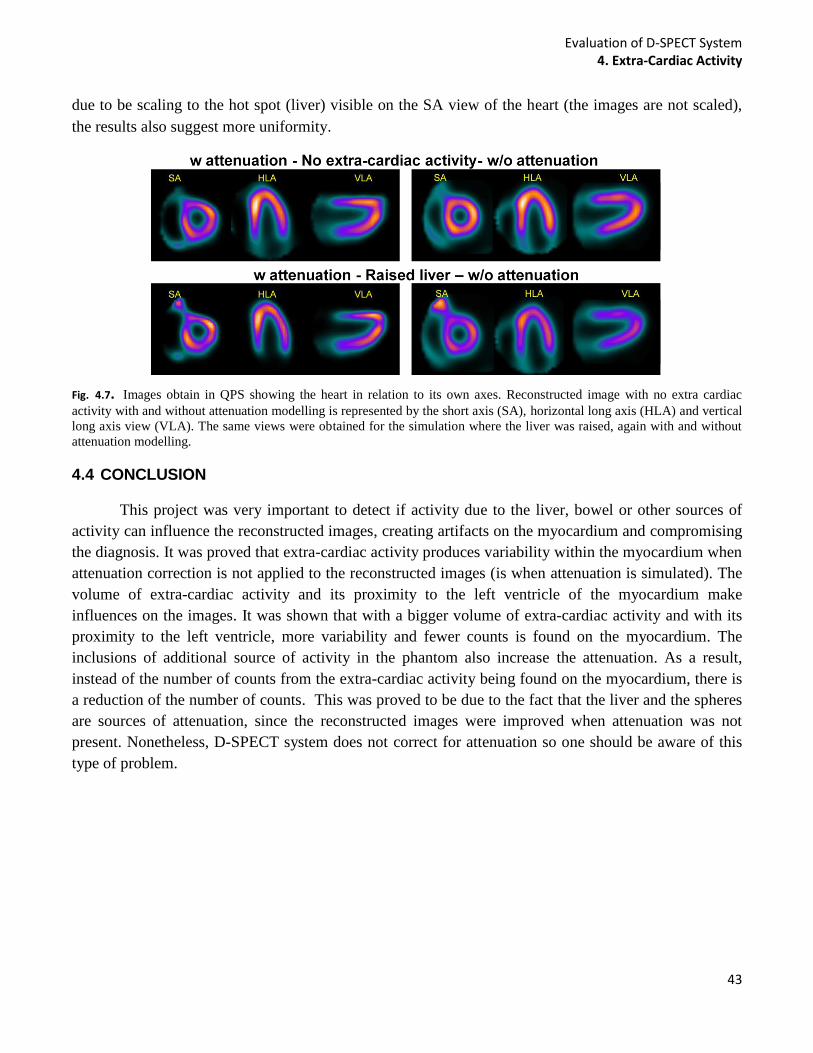
Evaluation of D-SPECT System 4. Extra-Cardiac Activity
43
due to be scaling to the hot spot (liver) visible on the SA view of the heart (the images are not scaled),
the results also suggest more uniformity.
Fig. 4.7. Images obtain in QPS showing the heart in relation to its own axes. Reconstructed image with no extra cardiac
activity with and without attenuation modelling is represented by the short axis (SA), horizontal long axis (HLA) and vertical
long axis view (VLA). The same views were obtained for the simulation where the liver was raised, again with and without
attenuation modelling.
4.4 CONCLUSION
This project was very important to detect if activity due to the liver, bowel or other sources of
activity can influence the reconstructed images, creating artifacts on the myocardium and compromising
the diagnosis. It was proved that extra-cardiac activity produces variability within the myocardium when
attenuation correction is not applied to the reconstructed images (is when attenuation is simulated). The
volume of extra-cardiac activity and its proximity to the left ventricle of the myocardium make
influences on the images. It was shown that with a bigger volume of extra-cardiac activity and with its
proximity to the left ventricle, more variability and fewer counts is found on the myocardium. The
inclusions of additional source of activity in the phantom also increase the attenuation. As a result,
instead of the number of counts from the extra-cardiac activity being found on the myocardium, there is
a reduction of the number of counts. This was proved to be due to the fact that the liver and the spheres
are sources of attenuation, since the reconstructed images were improved when attenuation was not
present. Nonetheless, D-SPECT system does not correct for attenuation so one should be aware of this
type of problem.
Evaluation of D-SPECT System 5. Tracer Kinetics
44
5 TRACER KINETICS
5.1 AIM
The D-SPECT system also allows for dynamic acquisition, and clinical dynamic exams are
nowadays a reality. It has been proved that quantitative kinetic analysis of dynamic cardiac SPECT, has
potential to obtain images with better contrast between healthy and diseased tissue, when compared with
a static image. Nevertheless, the radiopharmaceutical distribution is usually changing during the
acquisition process, creating some inconsistencies in the projection data due to the moving gantry, and
consequently, artifacts on the images, potentially leading to biased parameter estimation due to
inconsistencies in the projections.
The D-SPECT system has a different geometry and acquisition mode when compared with a
conventional SPECT. Even though D-SPECT is a cardiac dedicated system, it is composed by 9
detectors, that are small and each detector could not see the whole heart at once. During dynamic
acquisition, D-SPECT is programmed to scan 10 views for frame, which means to create the first view
the detectors will be oriented in a specific position, detecting information from different parts of the
heart. Then, to obtain the second view all the detectors will move and detect other parts of the heart, all
different from each other. This would not be a problem if the activity on the heart is practically constant
during the all scan, however if the activity on the heart changes, that can leads to a mismatch of the
projections obtained from the detectors. This project aims to investigate if the cardiac dedicated system
in study also create inconsistent projections that lead to artifacts on the reconstructed images, due to
dynamic acquisitions. The project includes the study of different protocols, changing the time spent to
obtain a frame and changing the velocity of bolus injection. It is important to study different protocols in
order to understand what would create better reconstructed images with accurate information. The
protocol applied at The Institute of Nuclear Medicine (INM) consists of a 6 minutes scan, taking 6
sec/frame and 10 views for frame. Other protocols were studied such as the case of 3 sec/frame scan,
because in 6 seconds the number of frames are obtained are doubled and the activity change between
frames is less. Thus, it was expected to obtain more accurate results due to the increased number of
frames and less artifacts as a consequence of a reduction in activity changes. Reducing the velocity of
bolus injection could also reduce possible artifacts since activity is changing more slowing. This and
other protocols were simulated and analyzed in terms of affects created on the images due to the
dynamic acquisition.
5.2 METHODS AND MATERIALS
In a similar way, in relation to the previous studies, the methodology of this part of the work can
be visualized by the diagram in Fig. 5.1. Although in this case both camera and source will change and
all combinations will be studied. Also the Model Interface code had to be changed as going to be
explained later on this work.
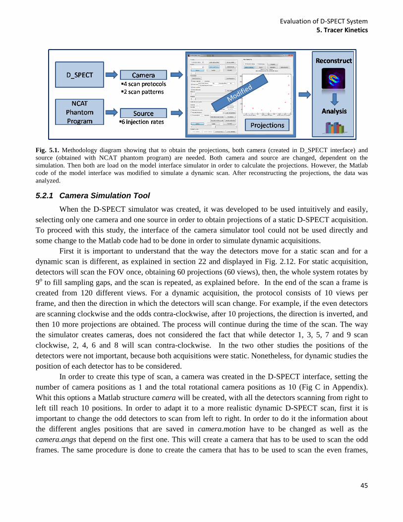
Evaluation of D-SPECT System 5. Tracer Kinetics
45
Fig. 5.1. Methodology diagram showing that to obtain the projections, both camera (created in D_SPECT interface) and
source (obtained with NCAT phantom program) are needed. Both camera and source are changed, dependent on the
simulation. Then both are load on the model interface simulator in order to calculate the projections. However, the Matlab
code of the model interface was modified to simulate a dynamic scan. After reconstructing the projections, the data was
analyzed.
5.2.1 Camera Simulation Tool
When the D-SPECT simulator was created, it was developed to be used intuitively and easily,
selecting only one camera and one source in order to obtain projections of a static D-SPECT acquisition.
To proceed with this study, the interface of the camera simulator tool could not be used directly and
some change to the Matlab code had to be done in order to simulate dynamic acquisitions.
First it is important to understand that the way the detectors move for a static scan and for a
dynamic scan is different, as explained in section 22 and displayed in Fig. 2.12. For static acquisition,
detectors will scan the FOV once, obtaining 60 projections (60 views), then, the whole system rotates by
9o to fill sampling gaps, and the scan is repeated, as explained before. In the end of the scan a frame is
created from 120 different views. For a dynamic acquisition, the protocol consists of 10 views per
frame, and then the direction in which the detectors will scan change. For example, if the even detectors
are scanning clockwise and the odds contra-clockwise, after 10 projections, the direction is inverted, and
then 10 more projections are obtained. The process will continue during the time of the scan. The way
the simulator creates cameras, does not considered the fact that while detector 1, 3, 5, 7 and 9 scan
clockwise, 2, 4, 6 and 8 will scan contra-clockwise. In the two other studies the positions of the
detectors were not important, because both acquisitions were static. Nonetheless, for dynamic studies the
position of each detector has to be considered.
In order to create this type of scan, a camera was created in the D-SPECT interface, setting the
number of camera positions as 1 and the total rotational camera positions as 10 (Fig C in Appendix).
Whit this options a Matlab structure camera will be created, with all the detectors scanning from right to
left till reach 10 positions. In order to adapt it to a more realistic dynamic D-SPECT scan, first it is
important to change the odd detectors to scan from left to right. In order to do it the information about
the different angles positions that are saved in camera.motion have to be changed as well as the
camera.angs that depend on the first one. This will create a camera that has to be used to scan the odd
frames. The same procedure is done to create the camera that has to be used to scan the even frames,
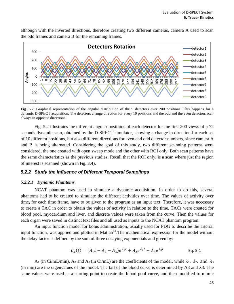
Evaluation of D-SPECT System 5. Tracer Kinetics
46
although with the inverted directions, therefore creating two different cameras, camera A used to scan
the odd frames and camera B for the remaining frames.
Fig. 5.2. Graphical representation of the angular distribution of the 9 detectors over 200 positions. This happens for a
dynamic D-SPECT acquisition. The detectors change direction for every 10 positions and the odd and the even detectors scan
always in opposite directions.
Fig. 5.2 illustrates the different angular positions of each detector for the first 200 views of a 72
seconds dynamic scan, obtained by the D-SPECT simulator, showing a change in direction for each set
of 10 different positions, but also different directions for even and odd detector numbers, since camera A
and B is being alternated. Considering the goal of this study, two different scanning patterns were
considered, the one created with open sweep mode and the other with ROI only. Both scan patterns have
the same characteristics as the previous studies. Recall that the ROI only, is a scan where just the region
of interest is scanned (shown in Fig. 3.4).
5.2.2 Study the Influence of Different Temporal Samplings
5.2.2.1 Dynamic Phantoms
NCAT phantom was used to simulate a dynamic acquisition. In order to do this, several
phantoms had to be created to simulate the different activities over time. The values of activity over
time, for each time frame, have to be given to the program as an input text. Therefore, it was necessary
to create a TAC in order to obtain the values of activity in relation to the time. TACs were created for
blood pool, myocardium and liver, and discrete values were taken from the curve. Then the values for
each organ were saved in distinct text files and all used as inputs to the NCAT phantom program.
An input function model for bolus administration, usually used for FDG to describe the arterial
input function, was applied and plotted in Matlab51
.The mathematical expression for the model without
the delay factor is defined by the sum of three decaying exponentials and given by:
Eq. 5.1
A1 (in Ci/mL/min), A2 and A3 (in Ci/mL) are the coefficients of the model, while 1, 2, and 3
(in min) are the eigenvalues of the model. The tail of the blood curve is determined by A3 and 3. The
same values were used as a starting point to create the blood pool curve, and then modified to mimic
-300
-200
-100
0
100
200
300
1
8
15
22
29
36
43
50
57
64
71
78
85
92
99
10
6
11
3
12
0
12
7
13
4
14
1
14
8
15
5
16
2
16
9
17
6
18
3
19
0
19
7
An
gle
s
Detectors Rotation detector1
detector2
detector3
detector4
detector5
detector6
detector7
detector8
detector9
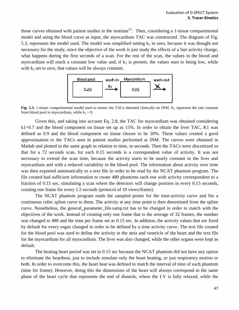
Evaluation of D-SPECT System 5. Tracer Kinetics
47
those curves obtained with patient studies in the institute52
. Then, considering a 1-tissue compartmental
model and using the blood curve as input, the myocardium TAC was constructed. The diagram of Fig.
5.3, represents the model used. The model was simplified setting k2 to zero, because it was thought not
necessary for the study, since the objective of the work is just study the effects of a fast activity change,
what happens during the first seconds of a scan. For the rest of the scan, the values in the blood and
myocardium will reach a constant low value and, if k2 is present, the values start to being low, while
with k2 set to zero, that values will be always constant.
Fig. 5.3. 1 tissue compartmental model used to mimic the TACs obtained clinically on INM. K1 represent the rate constant
from blood pool to myocardium, while k2 = 0.
Given this, and taking into account Eq. 2.8, the TAC for myocardium was obtained considering
k1=0.7 and the blood component on tissue set up as 15%. In order to obtain the liver TAC, K1 was
defined as 0.9 and the blood component on tissue choose to be 20%. These values created a good
approximation to the TACs seen in patient studies performed at INM. The curves were obtained in
Matlab and plotted in the same graph in relation to time, in seconds. Then the TACs were discretized so
that for a 72 seconds scan, for each 0.15 seconds is a correspondent value of activity. It was not
necessary to extend the scan time, because the activity starts to be nearly constant in the liver and
myocardium and with a reduced variability in the blood pool. The information about activity over time
was then exported automatically to a text file in order to be read by the NCAT phantom program. The
file created had sufficient information to create 480 phantoms each one with activity correspondent to a
fraction of 0.15 sec, simulating a scan where the detectors will change position in every 0.15 seconds,
creating one frame for every 1.5 seconds (protocol of 10 views/frame).
The NCAT phantom program reads the sampled points for the time-activity curve and fits a
continuous cubic spline curve to them. The activity at any time point is then determined from the spline
curve. Nonetheless, the general_parameter_file.samp.txt has to be changed in order to match with the
objectives of the work. Instead of creating only one frame that is the average of 32 frames, the number
was changed to 480 and the time per frame set as 0.15 sec. In addition, the activity values that are fixed
by default for every organ changed in order to be defined by a time activity curve. The text file created
for the blood pool was used to define the activity in the atria and ventricle of the heart and the text file
for the myocardium for all myocardium. The liver was also changed, while the other organs were kept as
default.
The beating heart period was set to 0.15 sec because the NCAT phantom did not have any option
to eliminate the heartbeat, just to include simulate only the heart beating, or just respiratory motion or
both. In order to overcome this, the heart beat was defined to match the interval of time of each phantom
(time for frame). However, doing this the dimensions of the heart will always correspond to the same
phase of the heart cycle that represents the end of diastole, where the LV is fully relaxed, while the
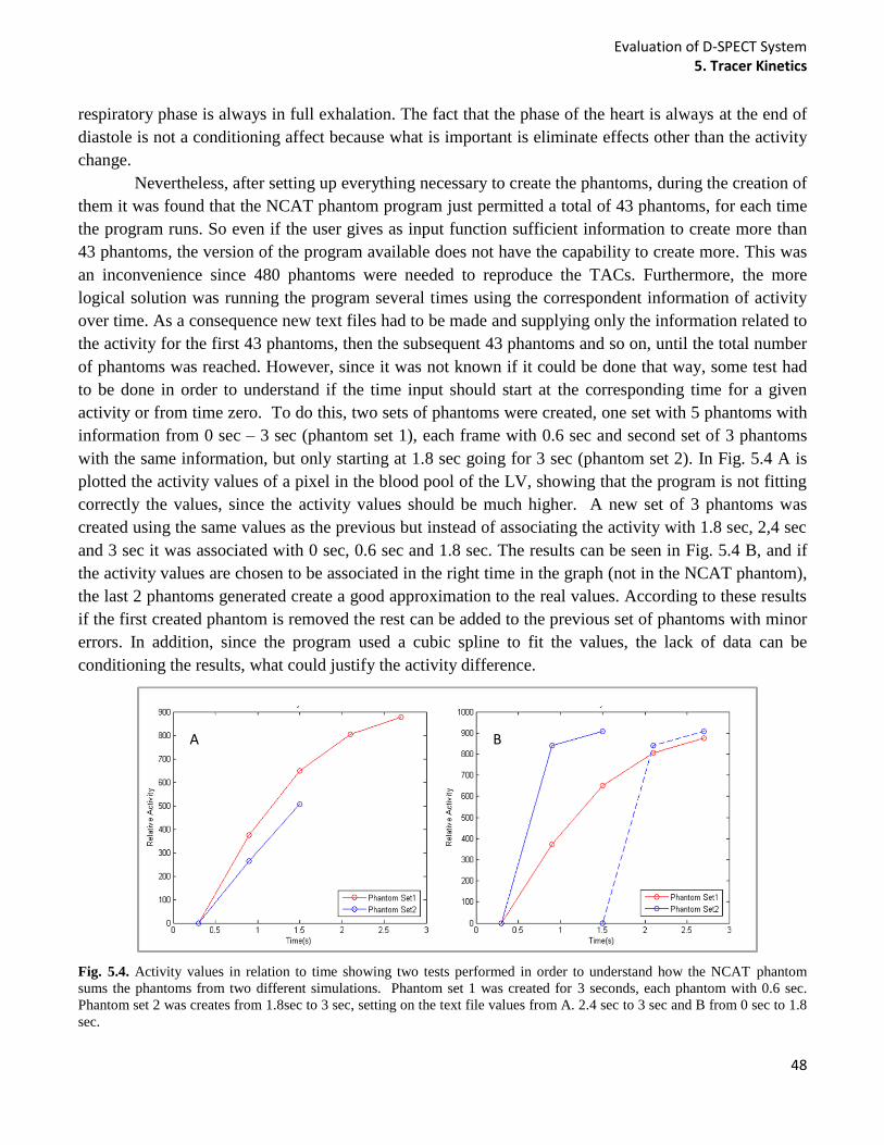
Evaluation of D-SPECT System 5. Tracer Kinetics
48
respiratory phase is always in full exhalation. The fact that the phase of the heart is always at the end of
diastole is not a conditioning affect because what is important is eliminate effects other than the activity
change.
Nevertheless, after setting up everything necessary to create the phantoms, during the creation of
them it was found that the NCAT phantom program just permitted a total of 43 phantoms, for each time
the program runs. So even if the user gives as input function sufficient information to create more than
43 phantoms, the version of the program available does not have the capability to create more. This was
an inconvenience since 480 phantoms were needed to reproduce the TACs. Furthermore, the more
logical solution was running the program several times using the correspondent information of activity
over time. As a consequence new text files had to be made and supplying only the information related to
the activity for the first 43 phantoms, then the subsequent 43 phantoms and so on, until the total number
of phantoms was reached. However, since it was not known if it could be done that way, some test had
to be done in order to understand if the time input should start at the corresponding time for a given
activity or from time zero. To do this, two sets of phantoms were created, one set with 5 phantoms with
information from 0 sec – 3 sec (phantom set 1), each frame with 0.6 sec and second set of 3 phantoms
with the same information, but only starting at 1.8 sec going for 3 sec (phantom set 2). In Fig. 5.4 A is
plotted the activity values of a pixel in the blood pool of the LV, showing that the program is not fitting
correctly the values, since the activity values should be much higher. A new set of 3 phantoms was
created using the same values as the previous but instead of associating the activity with 1.8 sec, 2,4 sec
and 3 sec it was associated with 0 sec, 0.6 sec and 1.8 sec. The results can be seen in Fig. 5.4 B, and if
the activity values are chosen to be associated in the right time in the graph (not in the NCAT phantom),
the last 2 phantoms generated create a good approximation to the real values. According to these results
if the first created phantom is removed the rest can be added to the previous set of phantoms with minor
errors. In addition, since the program used a cubic spline to fit the values, the lack of data can be
conditioning the results, what could justify the activity difference.
Fig. 5.4. Activity values in relation to time showing two tests performed in order to understand how the NCAT phantom
sums the phantoms from two different simulations. Phantom set 1 was created for 3 seconds, each phantom with 0.6 sec.
Phantom set 2 was creates from 1.8sec to 3 sec, setting on the text file values from A. 2.4 sec to 3 sec and B from 0 sec to 1.8
sec.
A B

Evaluation of D-SPECT System 5. Tracer Kinetics
49
Knowing this information, the second method (starting with time zero) was used to create new
text files with more data, to check if the error was reduced and if the data could be used for the propose
of the study. In order to do this 3 different text files were created. The first one, has information about
activity on the blood pool from 0 sec to 6.45 sec. Then the second file has the activity information
starting at 6 sec till 12.45 sec (but set to 0 sec until 6.45 sec on the text file) in order to verify if the cubic
spline created a good approximation of the values between 6sec and 6.45 sec. This creates two sets of
phantoms. An additional set was created starting at 12 sec and going till 18 seconds. Then the
corresponding files were created with activity information of the myocardium and liver, without
forgetting the time information have to start always in zero. Fig. 5.5 shows the resulting graph, plotting
the activity in the blood pool against time, again selecting a pixel in the blood pool of each phantom and
associating phantom set 2 and phantom set 3 to the right time in seconds.
Fig. 5.5. Initial 8 sec TAC of the blood pool obtained with 3 different simulations with NACT phantom. The value of a pixel
in the blood pool of each of the 120 phantom was plot (relative activity) in order to the correspondent time in seconds.
This proves that with more data the program fits a perfect curve, and extra phantom sets can be
added without any error. The black circle represents the mean value of activity over 10 phantoms.
Moreover, to create 480 phantoms the first three phantom sets were used, given a total of 120 phantoms
(40*3). To create the remaining 360 phantoms, 8 new sets with 43 phantoms each and 1 set with 16
phantoms where simulated and added to the previous sets (120 + 8*43 + 16 =480). Afterwards, the
created bin files were used to obtain the Matlab structures called source, and the phantom arms were
cropped, as in the previous studies.
With this information and selecting a pixel value on the blood pool, myocardium and liver, the
TACs on Fig. 5.6 were obtained. Again, the black circle represents the mean activity over 10 phantoms.
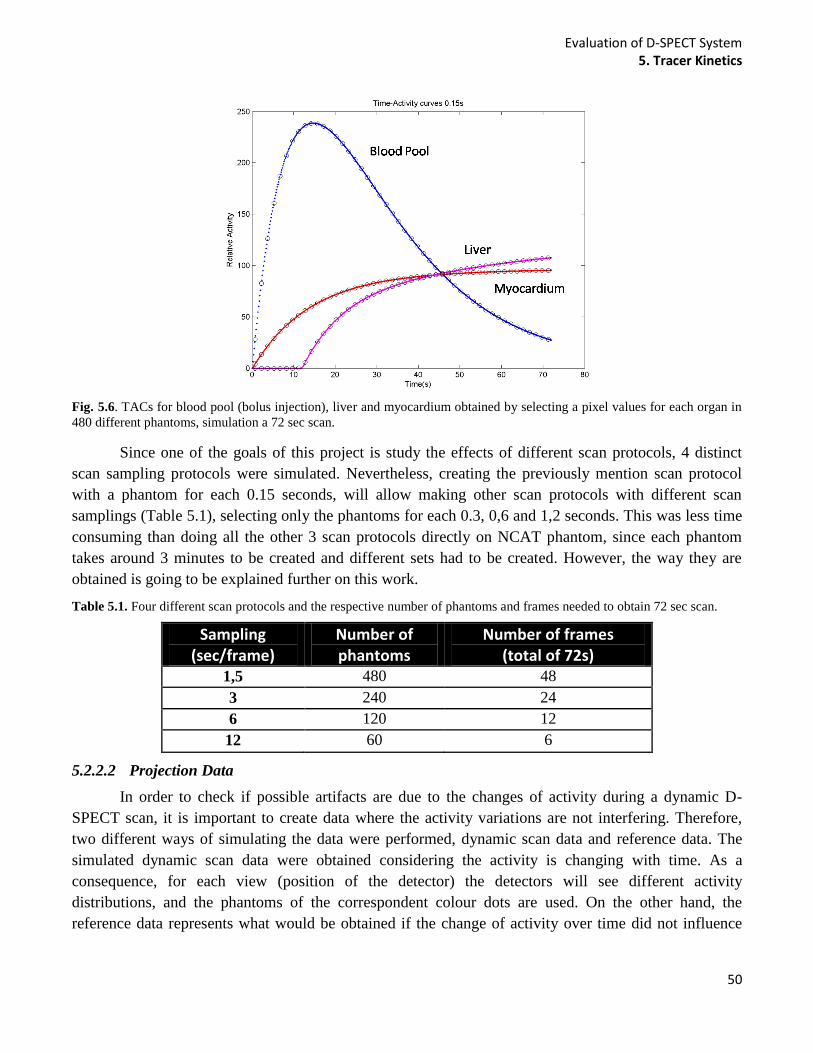
Evaluation of D-SPECT System 5. Tracer Kinetics
50
Fig. 5.6. TACs for blood pool (bolus injection), liver and myocardium obtained by selecting a pixel values for each organ in
480 different phantoms, simulation a 72 sec scan.
Since one of the goals of this project is study the effects of different scan protocols, 4 distinct
scan sampling protocols were simulated. Nevertheless, creating the previously mention scan protocol
with a phantom for each 0.15 seconds, will allow making other scan protocols with different scan
samplings (Table 5.1), selecting only the phantoms for each 0.3, 0,6 and 1,2 seconds. This was less time
consuming than doing all the other 3 scan protocols directly on NCAT phantom, since each phantom
takes around 3 minutes to be created and different sets had to be created. However, the way they are
obtained is going to be explained further on this work.
Table 5.1. Four different scan protocols and the respective number of phantoms and frames needed to obtain 72 sec scan.
Sampling (sec/frame)
Number of phantoms
Number of frames (total of 72s)
1,5 480 48
3 240 24
6 120 12
12 60 6
5.2.2.2 Projection Data
In order to check if possible artifacts are due to the changes of activity during a dynamic D-
SPECT scan, it is important to create data where the activity variations are not interfering. Therefore,
two different ways of simulating the data were performed, dynamic scan data and reference data. The
simulated dynamic scan data were obtained considering the activity is changing with time. As a
consequence, for each view (position of the detector) the detectors will see different activity
distributions, and the phantoms of the correspondent colour dots are used. On the other hand, the
reference data represents what would be obtained if the change of activity over time did not influence
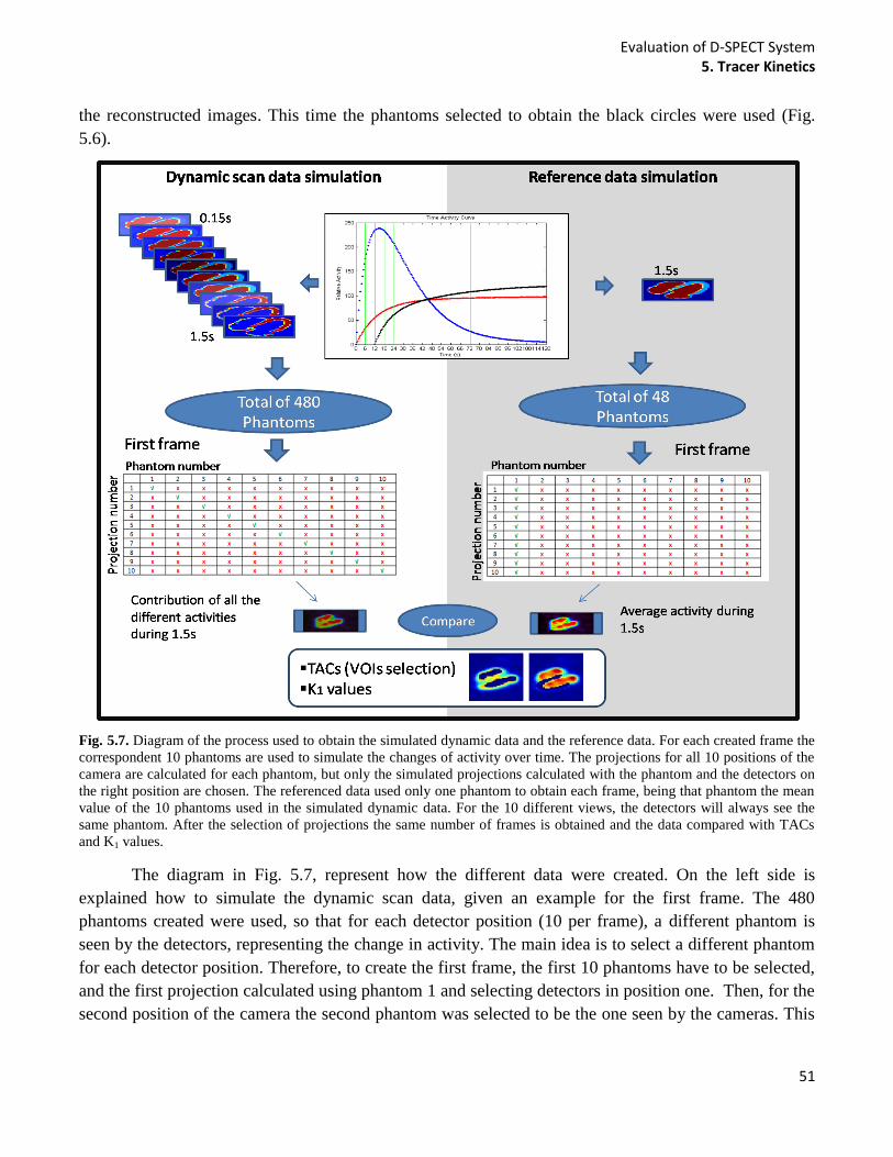
Evaluation of D-SPECT System 5. Tracer Kinetics
51
the reconstructed images. This time the phantoms selected to obtain the black circles were used (Fig.
5.6).
Fig. 5.7. Diagram of the process used to obtain the simulated dynamic data and the reference data. For each created frame the
correspondent 10 phantoms are used to simulate the changes of activity over time. The projections for all 10 positions of the
camera are calculated for each phantom, but only the simulated projections calculated with the phantom and the detectors on
the right position are chosen. The referenced data used only one phantom to obtain each frame, being that phantom the mean
value of the 10 phantoms used in the simulated dynamic data. For the 10 different views, the detectors will always see the
same phantom. After the selection of projections the same number of frames is obtained and the data compared with TACs
and K1 values.
The diagram in Fig. 5.7, represent how the different data were created. On the left side is
explained how to simulate the dynamic scan data, given an example for the first frame. The 480
phantoms created were used, so that for each detector position (10 per frame), a different phantom is
seen by the detectors, representing the change in activity. The main idea is to select a different phantom
for each detector position. Therefore, to create the first frame, the first 10 phantoms have to be selected,
and the first projection calculated using phantom 1 and selecting detectors in position one. Then, for the
second position of the camera the second phantom was selected to be the one seen by the cameras. This
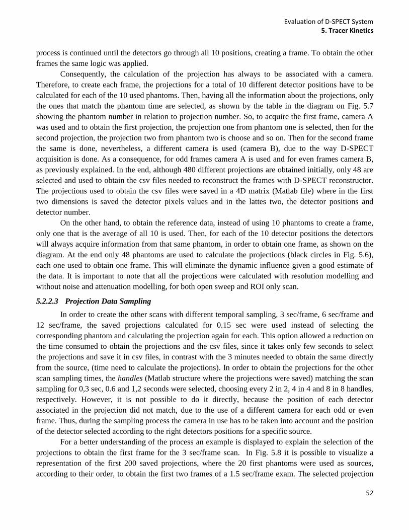
Evaluation of D-SPECT System 5. Tracer Kinetics
52
process is continued until the detectors go through all 10 positions, creating a frame. To obtain the other
frames the same logic was applied.
Consequently, the calculation of the projection has always to be associated with a camera.
Therefore, to create each frame, the projections for a total of 10 different detector positions have to be
calculated for each of the 10 used phantoms. Then, having all the information about the projections, only
the ones that match the phantom time are selected, as shown by the table in the diagram on Fig. 5.7
showing the phantom number in relation to projection number. So, to acquire the first frame, camera A
was used and to obtain the first projection, the projection one from phantom one is selected, then for the
second projection, the projection two from phantom two is choose and so on. Then for the second frame
the same is done, nevertheless, a different camera is used (camera B), due to the way D-SPECT
acquisition is done. As a consequence, for odd frames camera A is used and for even frames camera B,
as previously explained. In the end, although 480 different projections are obtained initially, only 48 are
selected and used to obtain the csv files needed to reconstruct the frames with D-SPECT reconstructor.
The projections used to obtain the csv files were saved in a 4D matrix (Matlab file) where in the first
two dimensions is saved the detector pixels values and in the lattes two, the detector positions and
detector number.
On the other hand, to obtain the reference data, instead of using 10 phantoms to create a frame,
only one that is the average of all 10 is used. Then, for each of the 10 detector positions the detectors
will always acquire information from that same phantom, in order to obtain one frame, as shown on the
diagram. At the end only 48 phantoms are used to calculate the projections (black circles in Fig. 5.6),
each one used to obtain one frame. This will eliminate the dynamic influence given a good estimate of
the data. It is important to note that all the projections were calculated with resolution modelling and
without noise and attenuation modelling, for both open sweep and ROI only scan.
5.2.2.3 Projection Data Sampling
In order to create the other scans with different temporal sampling, 3 sec/frame, 6 sec/frame and
12 sec/frame, the saved projections calculated for 0.15 sec were used instead of selecting the
corresponding phantom and calculating the projection again for each. This option allowed a reduction on
the time consumed to obtain the projections and the csv files, since it takes only few seconds to select
the projections and save it in csv files, in contrast with the 3 minutes needed to obtain the same directly
from the source, (time need to calculate the projections). In order to obtain the projections for the other
scan sampling times, the handles (Matlab structure where the projections were saved) matching the scan
sampling for 0,3 sec, 0.6 and 1,2 seconds were selected, choosing every 2 in 2, 4 in 4 and 8 in 8 handles,
respectively. However, it is not possible to do it directly, because the position of each detector
associated in the projection did not match, due to the use of a different camera for each odd or even
frame. Thus, during the sampling process the camera in use has to be taken into account and the position
of the detector selected according to the right detectors positions for a specific source.
For a better understanding of the process an example is displayed to explain the selection of the
projections to obtain the first frame for the 3 sec/frame scan. In Fig. 5.8 it is possible to visualize a
representation of the first 200 saved projections, where the 20 first phantoms were used as sources,
according to their order, to obtain the first two frames of a 1.5 sec/frame exam. The selected projection
Evaluation of D-SPECT System 5. Tracer Kinetics
53
to obtain the first frame for a 1.5 sec/frame was showed in Fig. 5.7, although, if one wants to simulate a
3 sec/frame scan, without calculating the projections again, the only important projections are the one
whose used source in every 0.3 seconds (shadowed columns). That means that it is just important to
select 2 in 2 projections, the 2nd
projection, and the 4th
and so on, till the 120th
. However, due to the fact
that every projection is associated with a camera position the direct sampling would not be correct.
Looking at the example in diagram (Fig. 5.8), the first 5 phantom selected will be associated with the
first camera position since the camera A was used to calculate projections for 1.5sec/frame scan.
Nevertheless, for phantom 6 to 10 the camera in use is B, but it should stay the same, camera A. Since
camera A and B have the same angles information but starting in opposite sides, the correspondent
angles have to be chosen to match the remaining angle positions. That is why projections 5 to 1 were
selected. The same was performed to obtain the remaining projections till the end of the scan. The whole
process was coded in order to be automated in Matlab. The same logic was used to obtain the projection
for the other two scan samplings, however two new Matlab scrips had to be created given that the
sampling for the other two scan samplings were very different. The representation for 6 sec/frame can be
found in Fig. D in appendix.
Fig. 5.8. Representation of the projections selected to create a 3 sec/frame scan, using the saved projections calculated to create de 1.5 sec/frame scan. The first table represent the available saved projection needed to create the first frame of 1.5sec/frame scan, being associated with camera A. The shadowed columns represent the selected the direct sampling selection while the right symbols represent the selected projection. The second table represent the same but for frame 2 of 1.5 sec/frame, being the camera B associated with the projections.
Evaluation of D-SPECT System 5. Tracer Kinetics
54
To create the reference data for the other scan protocols the process was slightly different. In this
situation the projections had to be calculated again, since each phantom corresponds to the average over
10 phantoms of 0.15 sec. Therefore, the phantoms corresponding to each 0.3sec, 0.6 sec and 1.2 sec are
chosen and then the average over 10 phantoms is calculated for all the three sampling options. Then the
projections were calculated in the same way as the 1.5 sec/frame scan protocol. Even though calculating
again the projections is time consuming, it will be 10 times faster than obtaining the projections of
dynamic scan data.
5.2.3 Study the Influence of Different Injections Rates
5.2.3.1 Dynamic Phantoms
It was also important to study the effect of different injection rates to understand if faster
injections rates create similar images to the ones when the injection of the radiotracer is slower. In order
to create different injection rates, the same sources were used. However, extra phantoms had to be
created in order to create a faster injection for the same scan time, 72 seconds using the same scan
sampling of 0.15 sec/frame.
As explain previously 12 x 3 distinct text files were created with the objective of reproducing a
dynamic NCAT phantom. To obtain the faster injection rate (injection rate 3) each phantom to 0.15 sec
was considered to correspond to 0.1 sec, which means 240 extra phantoms had to be added. In terms of
files needed, 6 new text files were created for each dynamic organ (6 x 3). 5 text files to create 43
phantoms each and the last to create 25 ((5*43) + 25 = 240), giving a total of 720 phantoms, reproducing
a 72 sec/scan. Nevertheless, to obtain a 15 sec/frame scan the 0.1 sec phantoms had to be transformed in
0.15 sec phantoms. The sampling does not allow the direct use of the phantoms, so to create the first
phantom, the activity after 0.15 sec will be the mean activity between the 0.1 sec phantom and the 0.2
sec phantom, then the 0.3 sec phantom was picked directly, but then to create the phantom after 0.45sec
the average between phantoms had to be calculated. This process is done till the end of the scan to
obtain the correct sampling. Considering that the process of creating new phantoms is very time
consuming and for the project aim the most important phase of the scan is the beginning, thus no more
phantoms were created.
Furthermore, 3 more injection rates were obtained using the available phantoms. Obviously, with
only this information it is not possible to create injection rates with information to create a 72 seconds
scan. For the new rates, rate 4, rate 5 and rate 6), the 0.15 sec phantoms were considered to correspond
to a 0.05 sec, 0.025 sec and 0.01 sec respectively. In order to obtain the corresponding 0.15 sec/frame
scan, only the corresponding phantoms are chosen to create the new simulation. Obviously, the number
of phantoms is reduced considerably, especially for the case where each phantom will correspond to
0.01 sec. This means for every 15 phantoms picking only one for the simulations. In appendix Fig E, it
is possible to visualize the logic applied to the sampling process to create the different injection rates,
from rate 3 to rate 6).
In Fig. 5.9 is represented the TACs for blood pool for each of the 6 injection rates created. While
for the first 3 injection rates the number of phantoms for each scan samplings was the same, since the
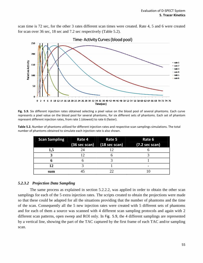
Evaluation of D-SPECT System 5. Tracer Kinetics
55
scan time is 72 sec, for the other 3 rates different scan times were created. Rate 4, 5 and 6 were created
for scan over 36 sec, 18 sec and 7.2 sec respectively (Table 5.2).
Fig. 5.9. Six different injection rates obtained selecting a pixel value on the blood pool of several phantoms. Each curve represents a pixel value on the blood pool for several phantoms, for six different sets of phantoms. Each set of phantom represent different injection rates, from rate 1 (slowest) to rate 6 (faster).
Table 5.2. Number of phantoms utilized for different injection rates and respective scan samplings simulations. The total number of phantoms obtained to simulate each injection rate is also shown.
5.2.3.2 Projection Data Sampling
The same process as explained in section 5.2.2.2, was applied in order to obtain the other scan
samplings for each of the 5 extra injection rates. The scripts created to obtain the projections were made
so that these could be adapted for all the situations providing that the number of phantoms and the time
of the scan. Consequently all the 5 new injection rates were created with 5 different sets of phantoms
and for each of them a source was scanned with 4 different scan sampling protocols and again with 2
different scan patterns, open sweep and ROI only. In Fig. 5.9, the 4 different samplings are represented
by a vertical line, showing the part of the TAC captured by the first frame of each TAC and/or sampling
scan.
Scan Sampling Rate 4 (36 sec scan)
Rate 5 (18 sec scan)
Rate 6 (7.2 sec scan)
1,5 24 12 6
3 12 6 3
6 6 3 1
12 3 1 -
sum 45 22 10
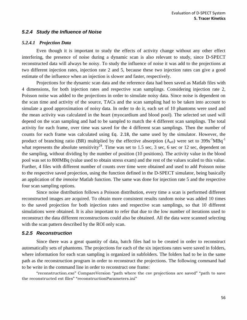
Evaluation of D-SPECT System 5. Tracer Kinetics
56
5.2.4 Study the Influence of Noise
5.2.4.1 Projection Data
Even though it is important to study the effects of activity change without any other effect
interfering, the presence of noise during a dynamic scan is also relevant to study, since D-SPECT
reconstructed data will always be noisy. To study the influence of noise it was add to the projections at
two different injection rates, injection rate 2 and 5, because these two injection rates can give a good
estimate of the influence when an injection is slower and faster, respectively.
Projections for the dynamic scan data and the reference data had been saved as Matlab files with
4 dimensions, for both injection rates and respective scan samplings. Considering injection rate 2,
Poisson noise was added to the projections in order to simulate noisy data. Since noise is dependent on
the scan time and activity of the source, TACs and the scan sampling had to be taken into account to
simulate a good approximation of noisy data. In order to do it, each set of 10 phantoms were used and
the mean activity was calculated in the heart (myocardium and blood pool). The selected set used will
depend on the scan sampling and had to be sampled to match the 4 different scan samplings. The total
activity for each frame, over time was saved for the 4 different scan samplings. Then the number of
counts for each frame was calculated using Eq. 2.18, the same used by the simulator. However, the
product of branching ratio (BR) multiplied by the effective absorption (Aeff) were set to 399s-1
MBq-1
what represents the absolute sensitivity24
. Time was set to 1.5 sec, 3 sec, 6 sec or 12 sec, dependent on
the sampling, without dividing by the number of position (10 positions). The activity value in the blood
pool was set to 800MBq (value used to obtain stress exam) and the rest of the values scaled to this value.
Further, 4 files with different number of counts over time were obtained and used to add Poisson noise
to the respective saved projection, using the function defined in the D-SPECT simulator, being basically
an application of the imnoise Matlab function. The same was done for injection rate 5 and the respective
four scan sampling options.
Since noise distribution follows a Poisson distribution, every time a scan is performed different
reconstructed images are acquired. To obtain more consistent results random noise was added 10 times
to the saved projection for both injection rates and respective scan samplings, so that 10 different
simulations were obtained. It is also important to refer that due to the low number of iterations used to
reconstruct the data different reconstructions could also be obtained. All the data were scanned selecting
with the scan pattern described by the ROI only scan.
5.2.5 Reconstruction
Since there was a great quantity of data, batch files had to be created in order to reconstruct
automatically sets of phantoms. The projections for each of the six injections rates were saved in folders,
where information for each scan sampling is organized in subfolders. The folders had to be in the same
path as the reconstruction program in order to reconstruct the projections. The following command had
to be write in the command line in order to reconstruct one frame:
“reconstruction.exe” CompareVersion “path where the csv projections are saved” “path to save
the reconstructed est files” “reconstructionParameters.ini”
Evaluation of D-SPECT System 5. Tracer Kinetics
57
The same command had to be written several time in the batch files to reconstruct all the
noiseless projections and the 10 sets of simulated noisy projections. Consequently different batch files
were needed.
The reconstructions were performed with 7 iterations without applying any fitting model or post
filters, as was done in the previous studies, with a filter between iterations. Nevertheless, instead of
using the swift mode, this information had to be unchecked on the interface of the program, because the
detectors scan always in the same directions without the 9o translation of the system (Fig B in
Attachment section). Since a batch files are being used, that information has to be changed in the
reconstructionparameters.ini file, where all reconstructing parameters and filter parameters can be
changed.
5.2.6 Analysis
5.2.6.1 Qualitative Analysis
All the data were analyzed visually and analytically, through the comparison between dynamic
scan data and the reference data. A visual evaluation could be a difficult task to perform because for
each scan simulation, several images are obtained, each representing a different time in the acquisition.
To organize all the data, a Matlab script was created allowing different ways to display and analyze the
results. Visualizing the obtained frames for both dynamic scan and reference scan for a specific injection
rate and scan sampling was one of the options, since it could be interesting to check during the scan time
if any artifact appears, not just in the initial seconds but also near the end where the activity is low and
almost constant. A more interesting analysis could be visualizing the data over a chosen 12 sec for all 4
scan samplings of a specific injection rate. A clinical view was also available to check if other artifacts
could be found.
In Fig. 5.10, the diagram shows how the data analysis script was organized. Selecting c) allows
the visualization of the data, while the other two options allow quantitative analysis, as going to be
explained in the next subchapter. For option a) the analysis is done for just one scan, meaning one
injection rate and a selected scan sampling. Option a) also plot an axial slice of reconstructed phantom
for each frame, for both dynamic and reference results and display the mask to select the blood pool and
myocardium used for that slice. The mask is different depending on the selected option, because the
analysis could be done for a 2D slice based on intensity or by a pre-defined mask, or a 3D mask based
on intensity. On the other hand selection b) is more useful to obtain the data for a quantitative analysis,
since no images are plotted. This information is going to be explained on the next subchapter.
For qualitative analysis option c), there is no need to select a VOI (mask), so the choice of an
injection rate scan is the first option to be selected, followed by the selection of the scan pattern (open
sweep or ROI only). If option a) and b) the scan sampling have to be chosen, although if it was c) all the
scan samplings are plotted, however the interval to analyze had to be given. Each interval corresponds to
12 sec, so if first 12 sec are selected, the first 12 seconds frames(s) for each scan sampling are plotted for
a specific axial slice. The type of scan has also to be selected and when both dynamic scan data and
reference data are plotted, the images shown for the dynamic scan are scaled to the respective maximal
value of the reference image.
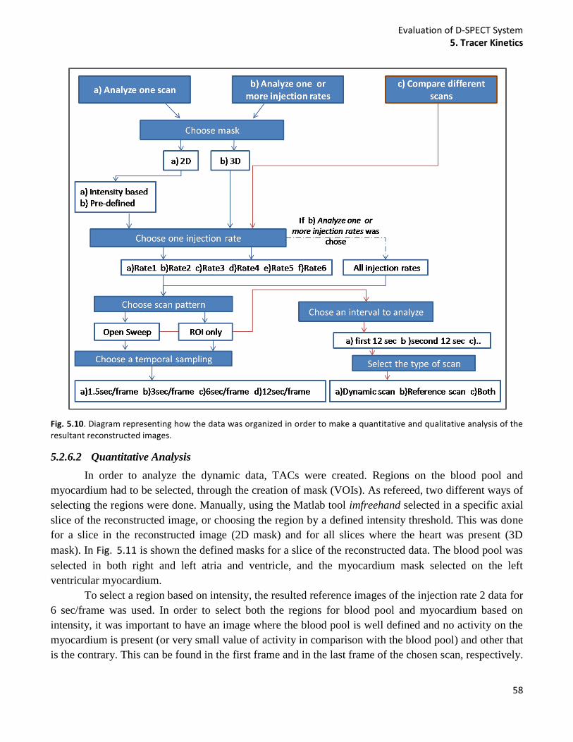
Evaluation of D-SPECT System 5. Tracer Kinetics
58
Fig. 5.10. Diagram representing how the data was organized in order to make a quantitative and qualitative analysis of the resultant reconstructed images.
5.2.6.2 Quantitative Analysis
In order to analyze the dynamic data, TACs were created. Regions on the blood pool and
myocardium had to be selected, through the creation of mask (VOIs). As refereed, two different ways of
selecting the regions were done. Manually, using the Matlab tool imfreehand selected in a specific axial
slice of the reconstructed image, or choosing the region by a defined intensity threshold. This was done
for a slice in the reconstructed image (2D mask) and for all slices where the heart was present (3D
mask). In Fig. 5.11 is shown the defined masks for a slice of the reconstructed data. The blood pool was
selected in both right and left atria and ventricle, and the myocardium mask selected on the left
ventricular myocardium.
To select a region based on intensity, the resulted reference images of the injection rate 2 data for
6 sec/frame was used. In order to select both the regions for blood pool and myocardium based on
intensity, it was important to have an image where the blood pool is well defined and no activity on the
myocardium is present (or very small value of activity in comparison with the blood pool) and other that
is the contrary. This can be found in the first frame and in the last frame of the chosen scan, respectively.
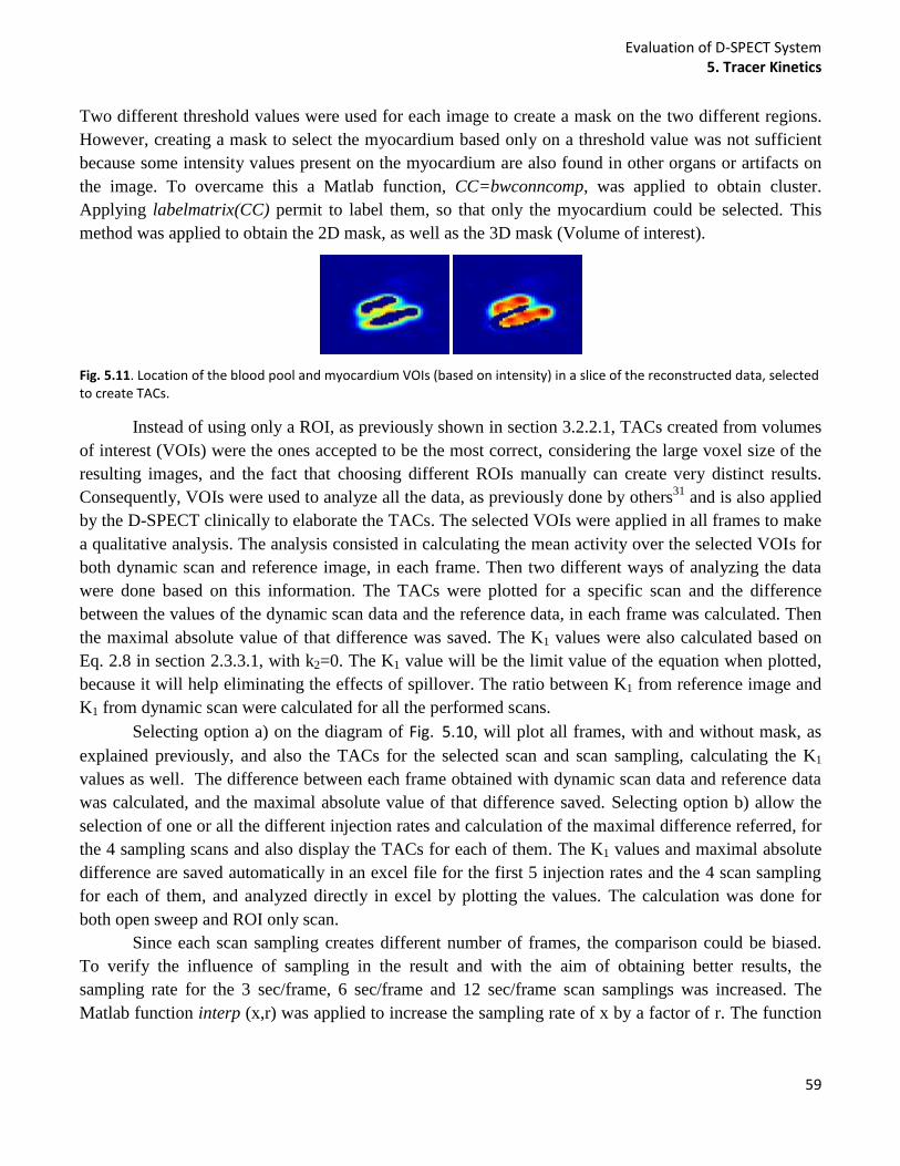
Evaluation of D-SPECT System 5. Tracer Kinetics
59
Two different threshold values were used for each image to create a mask on the two different regions.
However, creating a mask to select the myocardium based only on a threshold value was not sufficient
because some intensity values present on the myocardium are also found in other organs or artifacts on
the image. To overcame this a Matlab function, CC=bwconncomp, was applied to obtain cluster.
Applying labelmatrix(CC) permit to label them, so that only the myocardium could be selected. This
method was applied to obtain the 2D mask, as well as the 3D mask (Volume of interest).
Fig. 5.11. Location of the blood pool and myocardium VOIs (based on intensity) in a slice of the reconstructed data, selected to create TACs.
Instead of using only a ROI, as previously shown in section 3.2.2.1, TACs created from volumes
of interest (VOIs) were the ones accepted to be the most correct, considering the large voxel size of the
resulting images, and the fact that choosing different ROIs manually can create very distinct results.
Consequently, VOIs were used to analyze all the data, as previously done by others31
and is also applied
by the D-SPECT clinically to elaborate the TACs. The selected VOIs were applied in all frames to make
a qualitative analysis. The analysis consisted in calculating the mean activity over the selected VOIs for
both dynamic scan and reference image, in each frame. Then two different ways of analyzing the data
were done based on this information. The TACs were plotted for a specific scan and the difference
between the values of the dynamic scan data and the reference data, in each frame was calculated. Then
the maximal absolute value of that difference was saved. The K1 values were also calculated based on
Eq. 2.8 in section 2.3.3.1, with k2=0. The K1 value will be the limit value of the equation when plotted,
because it will help eliminating the effects of spillover. The ratio between K1 from reference image and
K1 from dynamic scan were calculated for all the performed scans.
Selecting option a) on the diagram of Fig. 5.10, will plot all frames, with and without mask, as
explained previously, and also the TACs for the selected scan and scan sampling, calculating the K1
values as well. The difference between each frame obtained with dynamic scan data and reference data
was calculated, and the maximal absolute value of that difference saved. Selecting option b) allow the
selection of one or all the different injection rates and calculation of the maximal difference referred, for
the 4 sampling scans and also display the TACs for each of them. The K1 values and maximal absolute
difference are saved automatically in an excel file for the first 5 injection rates and the 4 scan sampling
for each of them, and analyzed directly in excel by plotting the values. The calculation was done for
both open sweep and ROI only scan.
Since each scan sampling creates different number of frames, the comparison could be biased.
To verify the influence of sampling in the result and with the aim of obtaining better results, the
sampling rate for the 3 sec/frame, 6 sec/frame and 12 sec/frame scan samplings was increased. The
Matlab function interp (x,r) was applied to increase the sampling rate of x by a factor of r. The function
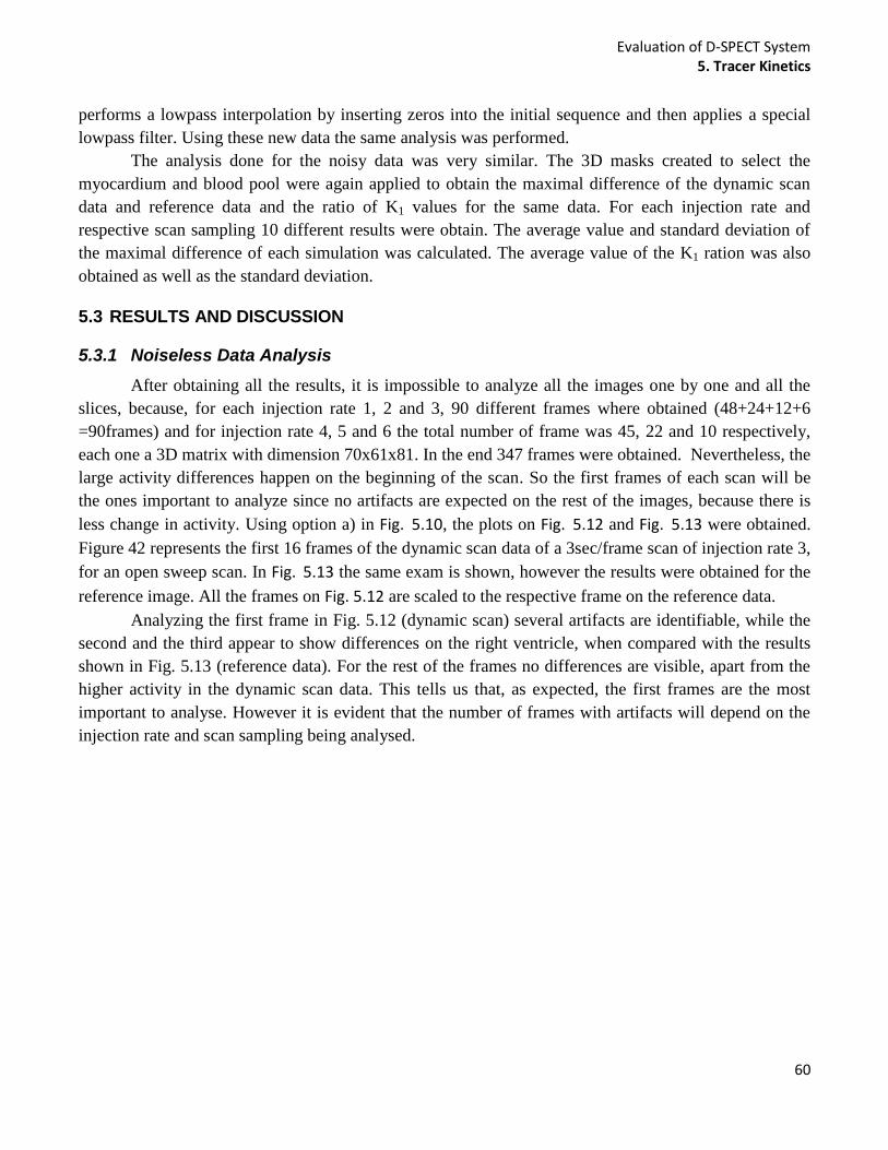
Evaluation of D-SPECT System 5. Tracer Kinetics
60
performs a lowpass interpolation by inserting zeros into the initial sequence and then applies a special
lowpass filter. Using these new data the same analysis was performed.
The analysis done for the noisy data was very similar. The 3D masks created to select the
myocardium and blood pool were again applied to obtain the maximal difference of the dynamic scan
data and reference data and the ratio of K1 values for the same data. For each injection rate and
respective scan sampling 10 different results were obtain. The average value and standard deviation of
the maximal difference of each simulation was calculated. The average value of the K1 ration was also
obtained as well as the standard deviation.
5.3 RESULTS AND DISCUSSION
5.3.1 Noiseless Data Analysis
After obtaining all the results, it is impossible to analyze all the images one by one and all the
slices, because, for each injection rate 1, 2 and 3, 90 different frames where obtained (48+24+12+6
=90frames) and for injection rate 4, 5 and 6 the total number of frame was 45, 22 and 10 respectively,
each one a 3D matrix with dimension 70x61x81. In the end 347 frames were obtained. Nevertheless, the
large activity differences happen on the beginning of the scan. So the first frames of each scan will be
the ones important to analyze since no artifacts are expected on the rest of the images, because there is
less change in activity. Using option a) in Fig. 5.10, the plots on Fig. 5.12 and Fig. 5.13 were obtained.
Figure 42 represents the first 16 frames of the dynamic scan data of a 3sec/frame scan of injection rate 3,
for an open sweep scan. In Fig. 5.13 the same exam is shown, however the results were obtained for the
reference image. All the frames on Fig. 5.12 are scaled to the respective frame on the reference data.
Analyzing the first frame in Fig. 5.12 (dynamic scan) several artifacts are identifiable, while the
second and the third appear to show differences on the right ventricle, when compared with the results
shown in Fig. 5.13 (reference data). For the rest of the frames no differences are visible, apart from the
higher activity in the dynamic scan data. This tells us that, as expected, the first frames are the most
important to analyse. However it is evident that the number of frames with artifacts will depend on the
injection rate and scan sampling being analysed.
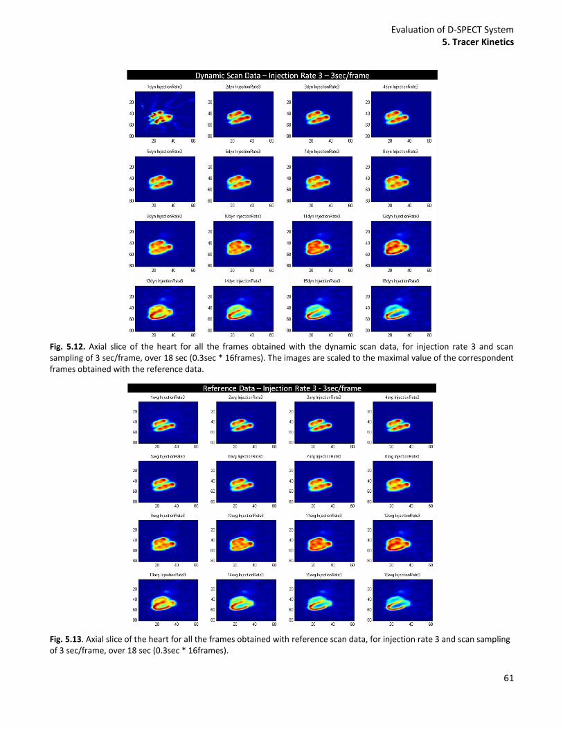
Evaluation of D-SPECT System 5. Tracer Kinetics
61
Fig. 5.12. Axial slice of the heart for all the frames obtained with the dynamic scan data, for injection rate 3 and scan sampling of 3 sec/frame, over 18 sec (0.3sec * 16frames). The images are scaled to the maximal value of the correspondent frames obtained with the reference data.
Fig. 5.13. Axial slice of the heart for all the frames obtained with reference scan data, for injection rate 3 and scan sampling of 3 sec/frame, over 18 sec (0.3sec * 16frames).
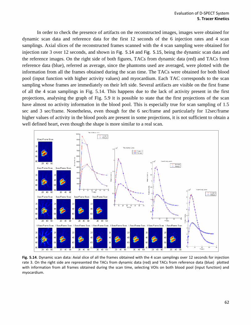
Evaluation of D-SPECT System 5. Tracer Kinetics
62
In order to check the presence of artifacts on the reconstructed images, images were obtained for
dynamic scan data and reference data for the first 12 seconds of the 6 injection rates and 4 scan
samplings. Axial slices of the reconstructed frames scanned with the 4 scan sampling were obtained for
injection rate 3 over 12 seconds, and shown in Fig. 5.14 and Fig. 5.15, being the dynamic scan data and
the reference images. On the right side of both figures, TACs from dynamic data (red) and TACs from
reference data (blue), referred as average, since the phantoms used are averaged, were plotted with the
information from all the frames obtained during the scan time. The TACs were obtained for both blood
pool (input function with higher activity values) and myocardium. Each TAC corresponds to the scan
sampling whose frames are immediately on their left side. Several artifacts are visible on the first frame
of all the 4 scan samplings in Fig. 5.14. This happens due to the lack of activity present in the first
projections, analysing the graph of Fig. 5.9 it is possible to state that the first projections of the scan
have almost no activity information in the blood pool. This is especially true for scan sampling of 1.5
sec and 3 sec/frame. Nonetheless, even though for the 6 sec/frame and particularly for 12sec/frame
higher values of activity in the blood pools are present in some projections, it is not sufficient to obtain a
well defined heart, even though the shape is more similar to a real scan.
Fig. 5.14. Dynamic scan data: Axial slice of all the frames obtained with the 4 scan samplings over 12 seconds for injection rate 3. On the right side are represented the TACs from dynamic data (red) and TACs from reference data (blue) plotted with information from all frames obtained during the scan time, selecting VOIs on both blood pool (input function) and myocardium.
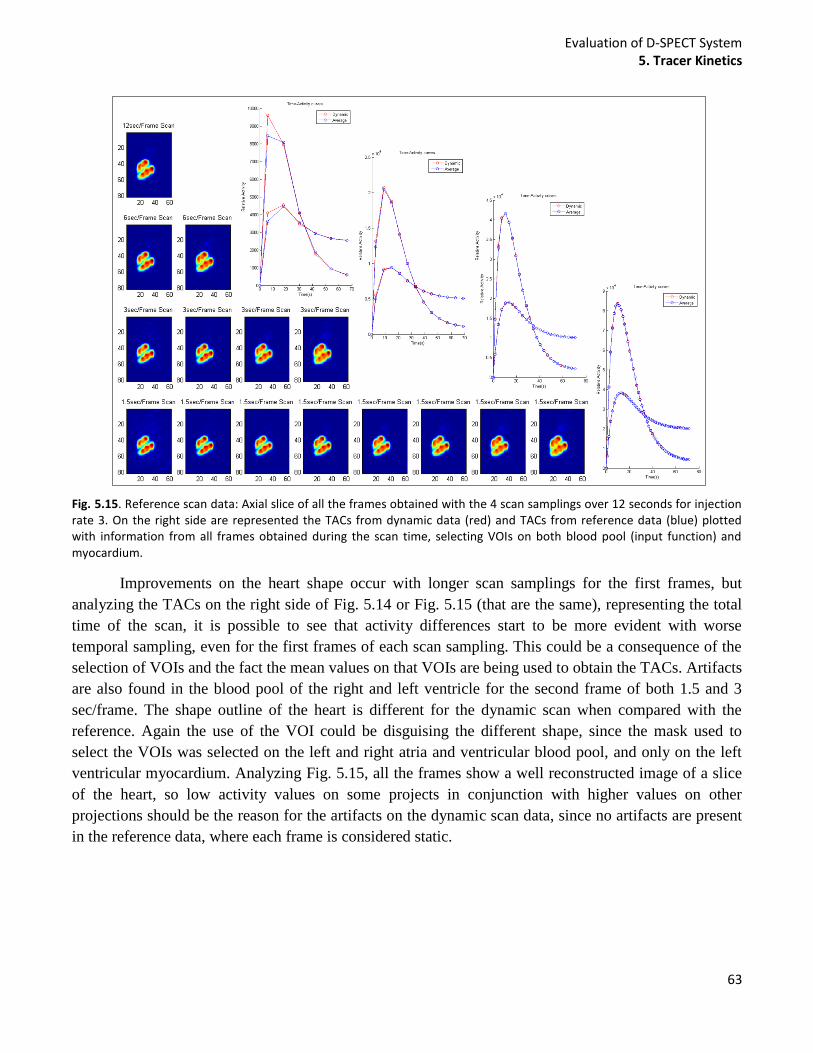
Evaluation of D-SPECT System 5. Tracer Kinetics
63
Fig. 5.15. Reference scan data: Axial slice of all the frames obtained with the 4 scan samplings over 12 seconds for injection rate 3. On the right side are represented the TACs from dynamic data (red) and TACs from reference data (blue) plotted with information from all frames obtained during the scan time, selecting VOIs on both blood pool (input function) and myocardium.
Improvements on the heart shape occur with longer scan samplings for the first frames, but
analyzing the TACs on the right side of Fig. 5.14 or Fig. 5.15 (that are the same), representing the total
time of the scan, it is possible to see that activity differences start to be more evident with worse
temporal sampling, even for the first frames of each scan sampling. This could be a consequence of the
selection of VOIs and the fact the mean values on that VOIs are being used to obtain the TACs. Artifacts
are also found in the blood pool of the right and left ventricle for the second frame of both 1.5 and 3
sec/frame. The shape outline of the heart is different for the dynamic scan when compared with the
reference. Again the use of the VOI could be disguising the different shape, since the mask used to
select the VOIs was selected on the left and right atria and ventricular blood pool, and only on the left
ventricular myocardium. Analyzing Fig. 5.15, all the frames show a well reconstructed image of a slice
of the heart, so low activity values on some projects in conjunction with higher values on other
projections should be the reason for the artifacts on the dynamic scan data, since no artifacts are present
in the reference data, where each frame is considered static.
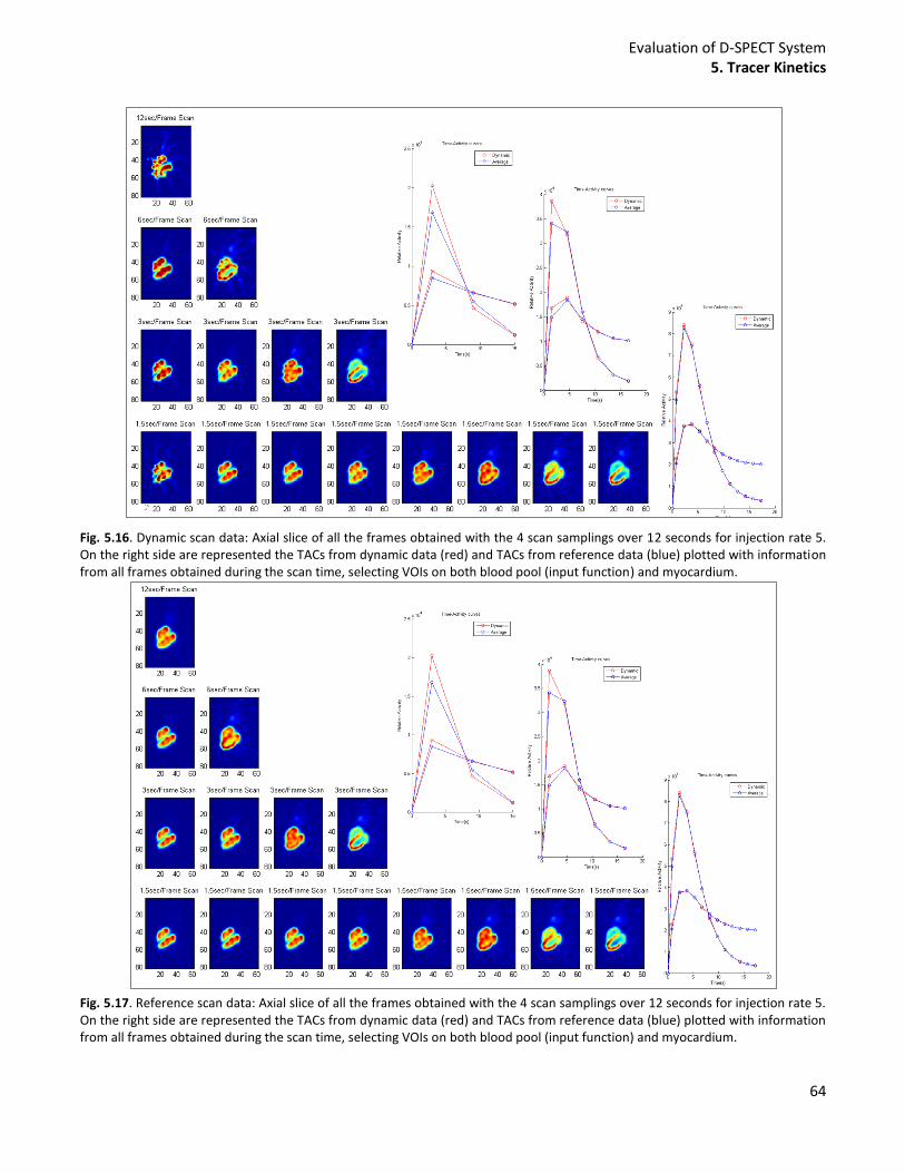
Evaluation of D-SPECT System 5. Tracer Kinetics
64
Fig. 5.16. Dynamic scan data: Axial slice of all the frames obtained with the 4 scan samplings over 12 seconds for injection rate 5. On the right side are represented the TACs from dynamic data (red) and TACs from reference data (blue) plotted with information from all frames obtained during the scan time, selecting VOIs on both blood pool (input function) and myocardium.
Fig. 5.17. Reference scan data: Axial slice of all the frames obtained with the 4 scan samplings over 12 seconds for injection rate 5. On the right side are represented the TACs from dynamic data (red) and TACs from reference data (blue) plotted with information from all frames obtained during the scan time, selecting VOIs on both blood pool (input function) and myocardium.

Evaluation of D-SPECT System 5. Tracer Kinetics
65
If an exam with a faster injection rate is analysed, some new information can be added to the
discussion. In Fig. 5.16 and Fig. 5.17, the same plots as were obtained for Fig. 5.14 and Fig. 5.15 were
made for injection rate 5. The artifacts present in all the first frames of the scans are not affecting the 6
sec/frame scan sampling in the same way as the others, since the shape did not suffer big differences
when compared with the reference image. Again Fig. 5.9 helps to understand the results. The first frame
of the 1.5sec and 3 sec/frame exams have the same problem as the previous, while for the 6 sec/frame
there is less projections derived from low activity sources. For the 12 sec/frame the reconstruction was
not efficient, not only because of the obtained projection on the beginning of the scan but also because
low values, after the slope, are being acquired. TACs for this specific injection rate show, once more,
that the difference between the dynamic scan data and the reference data (average) increases with more
time spent in each frame, in terms of mean activity in the VOIs. The TAC for the 12 sec/frame scan was
not obtained given that the injection rate 5 create an exam over 18 sec, what for a temporal sampling of
12 sec will create only one frame, what is not enough to create a time-activity curve. Additionally,
analysing the TACs the differences appear to be more evident for injection rate 5 than for injection rate
3, meaning faster injections produce worse results.
Fig. 5.18. Maximum value of the absolute difference between each point of the TACs obtained with dynamic scan data and
reference data, for an open sweep scan. The Maximum value is plot for 5 injection rates and respective scan samplings.
The maximal value of the absolute difference between the mean activity in a VOI of the dynamic
scan and a VOI in the reference data, for each scan are shown in Fig. 5.18, for an open sweep scan. The
mean activity in the VOIs (blood pool and myocardium) was calculated for each frame of the different
scans. The difference was normalized by the mean activity of the specific scan, and the values plotted on
the vertical axis of the graph. On the horizontal axis is represented the 5 injection rates and the
correspondent scan sampling. Graphs on Fig. 5.18 give a more specific assessment of all the possible
combinations (injection rates and scan samplings) and the affects in terms of maximal mean activity.
The graphs present important results for the open sweep scanned sources. They show that with small
0 0,05
0,1 0,15
0,2 0,25
0,3 0,35
0,4 0,45
0,5 0,55
0,6
Max
(|I
nt_
dyn
-In
t_av
g|/m
ean
(In
t_av
g))
Injection rate
TACs (Open sweep) Blood pool myocardium
Rate 1
Rate 2
Rate 5
Rate 4
Rate 3
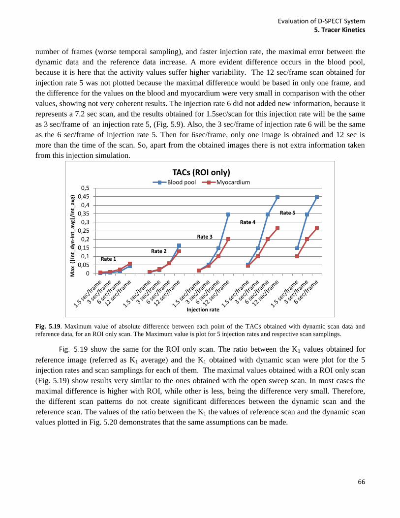
Evaluation of D-SPECT System 5. Tracer Kinetics
66
number of frames (worse temporal sampling), and faster injection rate, the maximal error between the
dynamic data and the reference data increase. A more evident difference occurs in the blood pool,
because it is here that the activity values suffer higher variability. The 12 sec/frame scan obtained for
injection rate 5 was not plotted because the maximal difference would be based in only one frame, and
the difference for the values on the blood and myocardium were very small in comparison with the other
values, showing not very coherent results. The injection rate 6 did not added new information, because it
represents a 7.2 sec scan, and the results obtained for 1.5sec/scan for this injection rate will be the same
as 3 sec/frame of an injection rate 5, (Fig. 5.9). Also, the 3 sec/frame of injection rate 6 will be the same
as the 6 sec/frame of injection rate 5. Then for 6sec/frame, only one image is obtained and 12 sec is
more than the time of the scan. So, apart from the obtained images there is not extra information taken
from this injection simulation.
Fig. 5.19. Maximum value of absolute difference between each point of the TACs obtained with dynamic scan data and
reference data, for an ROI only scan. The Maximum value is plot for 5 injection rates and respective scan samplings.
Fig. 5.19 show the same for the ROI only scan. The ratio between the K1 values obtained for
reference image (referred as K1 average) and the K1 obtained with dynamic scan were plot for the 5
injection rates and scan samplings for each of them. The maximal values obtained with a ROI only scan
(Fig. 5.19) show results very similar to the ones obtained with the open sweep scan. In most cases the
maximal difference is higher with ROI, while other is less, being the difference very small. Therefore,
the different scan patterns do not create significant differences between the dynamic scan and the
reference scan. The values of the ratio between the K1 the values of reference scan and the dynamic scan
values plotted in Fig. 5.20 demonstrates that the same assumptions can be made.
0
0,05
0,1
0,15
0,2
0,25
0,3
0,35
0,4
0,45
0,5
Max
(|I
nt_
dyn
-In
t_av
g|/I
nt_
avg)
Injection rate
TACs (ROI only) Blood pool Myocardium
Rate 1
Rate 2
Rate 5
Rate 4
Rate 3
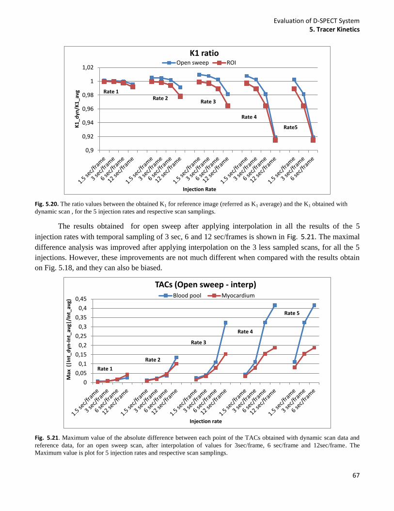
Evaluation of D-SPECT System 5. Tracer Kinetics
67
Fig. 5.20. The ratio values between the obtained K1 for reference image (referred as K1 average) and the K1 obtained with
dynamic scan , for the 5 injection rates and respective scan samplings.
The results obtained for open sweep after applying interpolation in all the results of the 5
injection rates with temporal sampling of 3 sec, 6 and 12 sec/frames is shown in Fig. 5.21. The maximal
difference analysis was improved after applying interpolation on the 3 less sampled scans, for all the 5
injections. However, these improvements are not much different when compared with the results obtain
on Fig. 5.18, and they can also be biased.
Fig. 5.21. Maximum value of the absolute difference between each point of the TACs obtained with dynamic scan data and
reference data, for an open sweep scan, after interpolation of values for 3sec/frame, 6 sec/frame and 12sec/frame. The
Maximum value is plot for 5 injection rates and respective scan samplings.
0,9
0,92
0,94
0,96
0,98
1
1,02
K1
_dyn
/K1
_avg
Injection Rate
K1 ratio Open sweep ROI
Rate 1 Rate 2
Rate5
Rate 4
Rate 3
0
0,05
0,1
0,15
0,2
0,25
0,3
0,35
0,4
0,45
Max
(|I
nt_
dyn
-In
t_av
g|/I
nt_
avg)
Injection rate
TACs (Open sweep - interp) Blood pool Myocardium
Rate 1
Rate 2
Rate 5
Rate 4
Rate 3
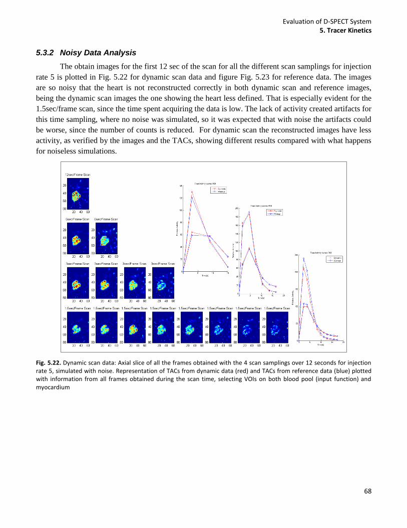
Evaluation of D-SPECT System 5. Tracer Kinetics
68
5.3.2 Noisy Data Analysis
The obtain images for the first 12 sec of the scan for all the different scan samplings for injection
rate 5 is plotted in Fig. 5.22 for dynamic scan data and figure Fig. 5.23 for reference data. The images
are so noisy that the heart is not reconstructed correctly in both dynamic scan and reference images,
being the dynamic scan images the one showing the heart less defined. That is especially evident for the
1.5sec/frame scan, since the time spent acquiring the data is low. The lack of activity created artifacts for
this time sampling, where no noise was simulated, so it was expected that with noise the artifacts could
be worse, since the number of counts is reduced. For dynamic scan the reconstructed images have less
activity, as verified by the images and the TACs, showing different results compared with what happens
for noiseless simulations.
Fig. 5.22. Dynamic scan data: Axial slice of all the frames obtained with the 4 scan samplings over 12 seconds for injection rate 5, simulated with noise. Representation of TACs from dynamic data (red) and TACs from reference data (blue) plotted with information from all frames obtained during the scan time, selecting VOIs on both blood pool (input function) and myocardium

Evaluation of D-SPECT System 5. Tracer Kinetics
69
Fig. 5.23. Reference scan data: Axial slice of all the frames obtained with the 4 scan samplings over 12 seconds for injection rate 5 simulated with noise. Representation of TACs from dynamic data (red) and TACs from reference data (blue) plotted with information from all frames obtained during the scan time, selecting VOIs on both blood pool (input function) and myocardium.
The qualitative analysis was again performed based on TACs and K1 values. Nevertheless two
graphs were obtained by plotting the maximal absolute difference between dynamic data and the
reference data. It is also shown a graph for maximal difference values on the blood pool (Fig. 5.24) and
for the myocardium (Fig. 5.25), both showing results from injection rate 2 and 5. It is possible to
observe that the 1.5 sec/frame exam is the scan that creates a higher difference between the dynamic
scan and the reference, contrary to what was shown for noiseless data. These results are visible for both
myocardium and blood pool. The larger difference can arise due to the noise, as a result of less time
spent during acquisition for each frame. In the blood pool, the results are improved for worse timing
samplings than 1.5 sec/frame, but the difference increased again for a 12sec/frame scan. Even though the
frames are less noisy, due to longer scan time for each frame, the worse time sampling seems to make a
bigger influence on the data. That increased different is more evident for the faster injection rate. On the
other hand, the conclusions taken from difference injection rates are the same. The maximal difference
is higher for a faster injection for any of the four scan sampling, and the standard deviation of the values
is also higher in all the cases for the injection rate 5. In the myocardium the same happen for injection
rate 2, but for injection rate 5 the maximal difference is reduced even more for 12sec/frame. This value
could not be considered because, as previously explained, only one frame was used to obtain the data,
and that frame corresponds to the first 12 seconds, where the activity on the myocardium is practically
non-existent in both reference and dynamic scan. The values of standard deviation represented by the
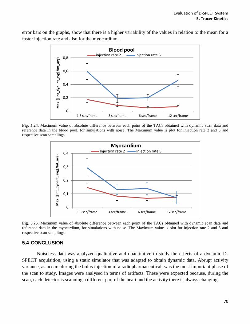
Evaluation of D-SPECT System 5. Tracer Kinetics
70
error bars on the graphs, show that there is a higher variability of the values in relation to the mean for a
faster injection rate and also for the myocardium.
Fig. 5.24. Maximum value of absolute difference between each point of the TACs obtained with dynamic scan data and
reference data in the blood pool, for simulations with noise. The Maximum value is plot for injection rate 2 and 5 and
respective scan samplings.
Fig. 5.25. Maximum value of absolute difference between each point of the TACs obtained with dynamic scan data and
reference data in the myocardium, for simulations with noise. The Maximum value is plot for injection rate 2 and 5 and
respective scan samplings.
5.4 CONCLUSION
Noiseless data was analyzed qualitative and quantitative to study the effects of a dynamic D-
SPECT acquisition, using a static simulator that was adapted to obtain dynamic data. Abrupt activity
variance, as occurs during the bolus injection of a radiopharmaceutical, was the most important phase of
the scan to study. Images were analysed in terms of artifacts. These were expected because, during the
scan, each detector is scanning a different part of the heart and the activity there is always changing.
0
0,2
0,4
0,6
0,8
1.5 sec/frame 3 sec/frame 6 sec/frame 12 sec/frame
Max
(|I
nt_
dyn
-In
t_av
g|/I
nt_
avg)
Blood pool injection rate 2 Injection rate 5
0
0,1
0,2
0,3
0,4
1.5 sec/frame 3 sec/frame 6 sec/frame 12 sec/frame
Max
(|I
nt_
dyn
-In
t_av
g|/I
nt_
avg)
Myocardium Injection rate 2 Injection rate 5
Evaluation of D-SPECT System 5. Tracer Kinetics
71
Since the reference data were considered as the true results, without the effect of dynamic
changes of activity, clinical conclusions can be drawn in order to improve the D-SPECT dynamic
protocol. If no noise is being modelled, results suggest that a better temporal sampling results in images
less affected by the dynamic process. This was proved because with better temporal sampling, the
difference between the mean values calculated in the blood pool and myocardium with the dynamic scan
and the reference is reduced. That difference is also less when the injection rate is slower. Artifacts were
found in the ventricles when the activity has lower values. This is not a problem in the absence of noise
or attenuation, however in a real D-SPECT these affects will be present and the number of counts will
be less. In addition, a slower injection can also create problems because the scan time may be longer and
the spillover affect can also get more problematic. It is important to notice that, since resolution is being
modelled, the calculation of the mean activity in each VOI will be biased due to errors associated with
partial volume discretization. The spillover effect occurs when some pixels in the myocardium VOI
contain partial components due to blood pool and vice-versa. When compared the myocardium curve of
reconstructed images with the real phantoms (example on Fig. 5.6) is clearly that some values of the
blood pool are taken into account in the myocardium VOI, even though the mask was choose to be the
tightness possible. Partial volume correction should be performed in order to correct the spillover effect
and allow a direct comparison with the real phantom. Correcting for spillover effect and comparing with
the real phantom could be a more correct way to analyze the data than the reference image, but partial
volume correction would be necessary.
There are other limitations of the study. The activity on the ventricle and atria of the heart were
considered as having only one value of activity. Obviously that does not happen that way because first
the activity starts to show up in the right ventricle and then goes to the left ventricle, then it starts to
disappear from the blood pool of the ventricles and starts to be seen in the myocardial wall surrounding
the left ventricle, after passing through the lungs. A more realistic simulation should be created in order
to obtain accurate results. That could be obtained using a different 1-tissue compartmental model for
each right ventricle and other with a delayed response representing the left ventricle.
Simulation with noise modelling showed some different conclusion, as expected, since noise is
dependent on activity and time of the scan. Results suggest that the data can be improved when the
injection rate is slower and the scan protocol acquired gets 3 to 6 sec/frame. The projections acquired
with 1.5 sec/frame protocol, were very noisy because of the lack of time available to acquire data from
the heart. More simulations should be performed with noise, including other injection rates simulations.
It is also important to note that activity on the myocardium is usually even less than 800MBq, for rest
tests using 99m
Tc Sestamibi (~ 400MBq). With reduced activity the number of counts will be even less,
possibly resulting in even worst results. However it is expected that the same conclusions can be drawn.
More studies should be performed to quantitatively know how different could be the results.
Evaluation of D-SPECT System 6. General Conclusion
72
6 GENERAL CONCLUSION
The current project was very important to evaluate the D-SPECT system, studying different
modes of acquiring the data with the new cardiac system. D-SPECT is now used in several clinics to
assess CAD and for clinical trials, so it was extremely important to verify if the system has limitations in
both static and dynamic acquisition.
The first study showed that choosing different scan patterns does not have much affect on the
reconstructed images of the heart, if the selected region is not too small. An acquisition scan with a very
small region showed higher variability on the myocardium and distortion in the reconstructed image of
the heart. The study suggests that instead of scanning with the clinical scan protocol, in which more time
is spent on a the selected region, the ROI only scan could be used. This will create a faster acquisition
with higher sensitivity to counts originating in the heart.
Truncating the data proved to be reliable even though is being acquired information just from the
heart. Nevertheless, if extra-cardiac activity is present the results can start to show some problems. Some
organs, such as liver or bowel, can be sources of extra-cardiac activity, which can be difficult to avoid.
Studying effects when just the ROI is scanned was performed for different situations. Results showed
that with an increased volume of extra-cardiac activity and with increased proximity to the myocardium,
higher variability on the left ventricle was found and also less detected counts. However, these are the
conclusion taken from simulation with attenuation modelling. When attenuation was not modelled, the
effects of variability and the decreased number of counts were reduced drastically, showing that extra-
cardiac activity does not damage the images, reconstructing the heart correctly. For this and as the
previous study, no noise was modelled, so it was possible to isolate the effects of scan patterns and
extra-cardiac activity, proving to create reliable reconstructed images of the heart in both cases.
Nevertheless more studies should be developed analysing the same affects in the presence of noise.
Validation of the data could also be useful to perform in the real D-SPECT with a physical phantom.
Apart from the factors that were studied to check possible artifacts on the reconstructed images
during a static scan, the selection of different scan patterns were also studied because they can be
problematic during a dynamic scan. The study of different protocols, changing the time for frame of the
acquisition and the rate of the bolus injection resulted in very interesting conclusions. If attenuation or
noise are not interfering the projections, simulation with better time sampling and slower bolus injection,
allow reconstructing the frames with more accurate parameter estimation. As a consequence, the best
protocol studied was found to be scanning with 1.5 sec/frame scanned an injection bolus taking more
than 72 sec for the activity pick be eliminated from the blood pool, and the activity there stays constant.
Despite, the fact that a scan is being performed at the same time is the activity was changing, artifacts on
the images were not increased, proving it is reliable to acquire dynamic data. The data acquired with
ROI only and with open sweep do not show very different results, so again in a similar way as what was
shown for the static D-SPECT acquisition, the different scan patterns acquired dynamically do not
affects the reconstructed data.

Evaluation of D-SPECT System 6. General Conclusion
73
These simulations were again calculated without noise in order to eliminate the effects of it.
Simulation with noise modelling showed different conclusion. Again the slowest injection bolus
produced better results, but acquisition with less time spend for frame was no longer producing the best
results, being the scan for 3 and 6 sec/frame getting less error differences. It is important to note that
these reduced temporal sampling would not be available with a conventional SPECT, that scans around
10 to 15 seconds in order to get a frame. This is a great advantage of this system, allowing to get more
information during a dynamic scan, creating more accurate TACs and obtaining a more precise
estimation of parameters.
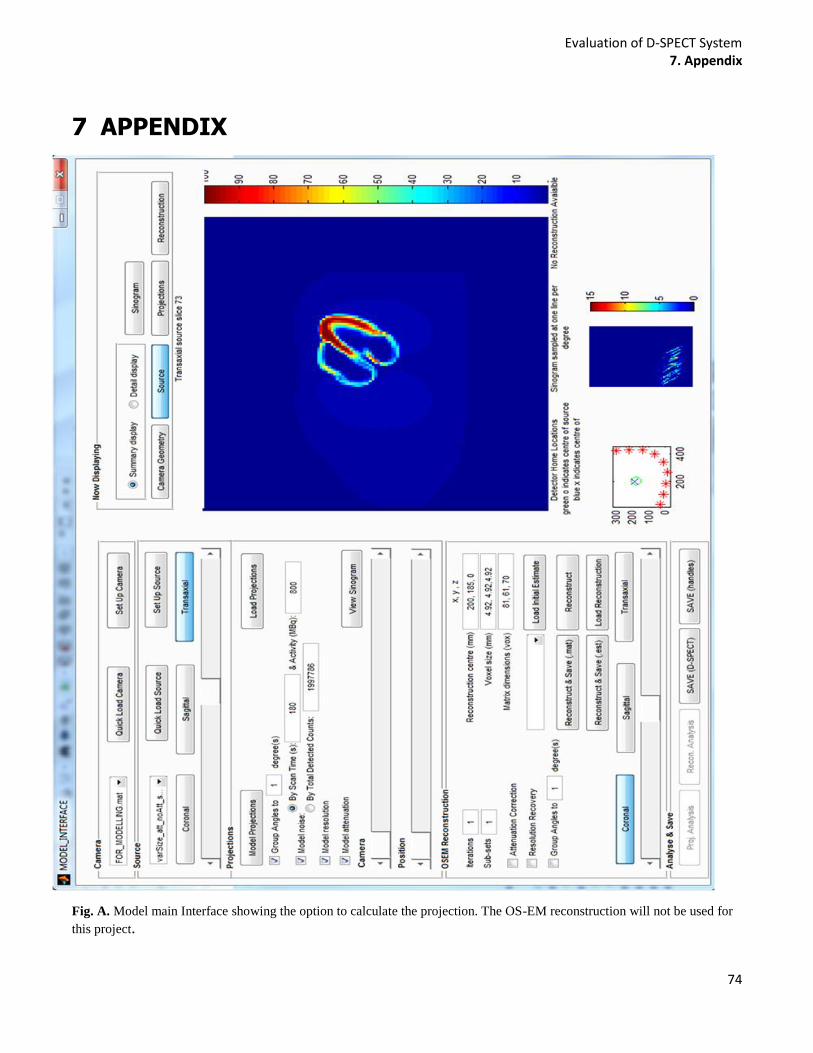
Evaluation of D-SPECT System 7. Appendix
74
7 APPENDIX
Fig. A. Model main Interface showing the option to calculate the projection. The OS-EM reconstruction will not be used for
this project.

Evaluation of D-SPECT System 7. Appendix
75
Fig.B. The reconstruction program from Spectrum Dynamics, used clinically.
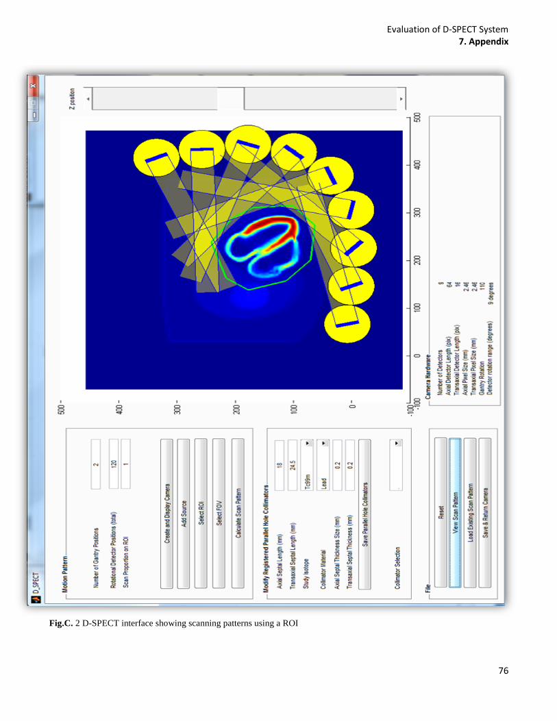
Evaluation of D-SPECT System 7. Appendix
76
Fig.C. 2 D-SPECT interface showing scanning patterns using a ROI
Evaluation of D-SPECT System 7. Appendix
77
Fig.D. Representation of the projections selected to create a 6 sec/frame scan, using the saved projections calculated to create
de 1.5 sec/frame scan. The first table represent the available saved projection needed to create the first frame of 1.5sec/frame
scan, being associated with camera A. The selection of projections was done using the same logic used to create the
3sec/frame scan.
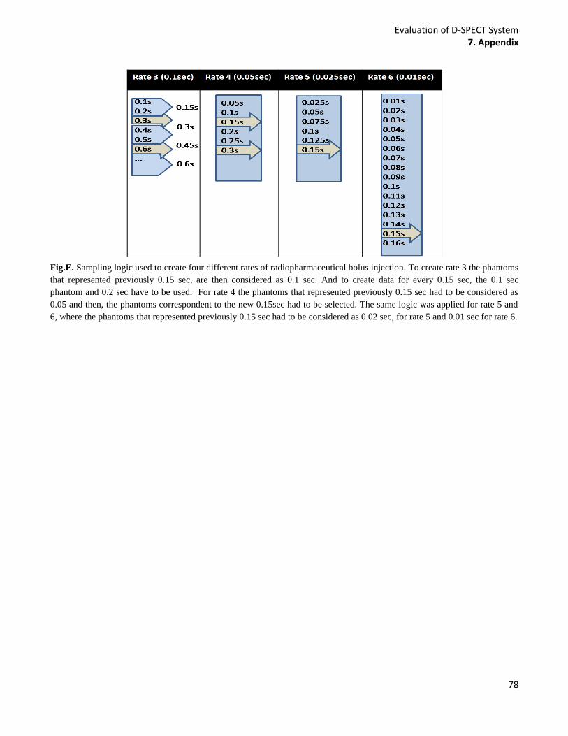
Evaluation of D-SPECT System 7. Appendix
78
Fig.E. Sampling logic used to create four different rates of radiopharmaceutical bolus injection. To create rate 3 the phantoms
that represented previously 0.15 sec, are then considered as 0.1 sec. And to create data for every 0.15 sec, the 0.1 sec
phantom and 0.2 sec have to be used. For rate 4 the phantoms that represented previously 0.15 sec had to be considered as
0.05 and then, the phantoms correspondent to the new 0.15sec had to be selected. The same logic was applied for rate 5 and
6, where the phantoms that represented previously 0.15 sec had to be considered as 0.02 sec, for rate 5 and 0.01 sec for rate 6.
Evaluation of D-SPECT System 7. Appendix
79
8 REFERENCES
1. Powsner RA, Powsner ER. Essential Nuclear Medicine Physics. Second edi. Blackwell Publishing
Ltd; 2006:1829–1841.
2. Zaidi H, Erwin WD. Quantitative Analysis in Nuclear Medicine Imaging. Springer; 2007:1401-1401.
3. Physics C on the M and I. Mathematics and Physics of Emerging Biomedical Imaging. National
Academy Press; 1996.
4. Bruyant PP. Analytic and Iterative Reconstruction Algorithms in SPECT *. October. 2002:1343-
1358.
5. Fred A. Mettler, Jr., md M, Milton J. Guiberteau M. Essentials of Nuclear Medicine Imaging.
ELSEVIER; 2006.
6. Khalil MM. Basic Sciences of Nuclear Medicine. Springer; 2010.
7. Hutton BE, Hudson HM, Beekman FJ. A clinical perspective of accelerated statistical reconstruction.
European Journal of Nuclear Medicine. 1997;24(7).
8. Wernick MN, Aarsvold JN. Emission Tomography: Fundamentals of PET and SPECT. 2004.
9. Zeng GL. Image reconstruction--a tutorial. Computerized medical imaging and graphics : the official
journal of the Computerized Medical Imaging Society. 2001;25(2):97-103. Available at:
http://www.ncbi.nlm.nih.gov/pubmed/11137785.
10. Vandenberghe S, D’Asseler Y, Van de Walle R, et al. Iterative reconstruction algorithms in nuclear
medicine. Computerized medical imaging and graphics : the official journal of the Computerized
Medical Imaging Society. 2001;25(2):105-11. Available at:
http://www.ncbi.nlm.nih.gov/pubmed/11137786.
11. Shepp L a, Vardi Y. Maximum likelihood reconstruction for emission tomography. IEEE
transactions on medical imaging. 1982;1(2):113-22. Available at:
http://www.ncbi.nlm.nih.gov/pubmed/18238264.
12. Hudson HM, S.Larkin R. Accelerated Image Reconstruction using Ordered Subsets of Projection
Data. 1994.
13. Gambhir SS, Berman DS, Ziffer J, et al. A novel high-sensitivity rapid-acquisition single-photon
cardiac imaging camera. Journal of nuclear medicine : official publication, Society of Nuclear Medicine.
2009;50(4):635-43. Available at: http://www.ncbi.nlm.nih.gov/pubmed/19339672. Accessed October
22, 2011.

Evaluation of D-SPECT System 7. Appendix
80
14. Slomka PJ, Patton J a, Berman DS, Germano G. Advances in technical aspects of myocardial
perfusion SPECT imaging. Journal of nuclear cardiology : official publication of the American Society
of Nuclear Cardiology. 16(2):255-76. Available at: http://www.ncbi.nlm.nih.gov/pubmed/19242769.
Accessed July 25, 2011.
15. Bonow RO. High-speed myocardial perfusion imaging: dawn of a new era in nuclear cardiology?
JACC. Cardiovascular imaging. 2008;1(2):164-6. Available at:
http://www.ncbi.nlm.nih.gov/pubmed/19356423. Accessed November 22, 2011.
16. Movahed A, Gnanasegaran G, Buscombe JR, Hall M. Integrating Cardiology for Nuclear Medicine
Physicians. Springer; 2009.
17. Gullberg GT. DYNAMIC SPECT IMAGING : EXPLORING A NEW FRONTIER IN MEDICAL
IMAGING Grant T . Gullberg. In: Lawrence Berkeley Nat. Lab. 2004:607-610.
18. Strauss HW, Miller DD, Wittry MD, et al. Society of Nuclear Medicine Procedure Guideline for
Myocardial Perfusion Imaging. Cardiovascular Imaging. 2002.
19. Klein RAN. Kinetic Model Based Factor Analysis of Cardiac 82 Rb PET Images for Improved
Accuracy of Quantitative Myocardial Blood Flow Measurement PhD degree in Electrical and Computer
Engineering. 2010;(May).
20. Ghosh P, Burckhardt DD. Expanding the Power of PET with syngo MBF. Siemens. 2010.
21. Jin M, Member S, Yang Y, et al. Fully 5D reconstruction of gated dynamic cardiac SPECT images.
Nuclear Science Symposium Conference Record. 2006;(3):3445-3448.
22. Cerqueira MD. Standardized Myocardial Segmentation and Nomenclature for Tomographic Imaging
of the Heart: A Statement for Healthcare Professionals From the Cardiac Imaging Committee of the
Council on Clinical Cardiology of the American Heart Association. Circulation. 2002;105(4):539-542.
Available at: http://circ.ahajournals.org/cgi/doi/10.1161/hc0402.102975. Accessed July 6, 2011.
23. Schepis T, Gaemperli O, Koepfli P, et al. Comparison of 64-slice CT with gated SPECT for
evaluation of left ventricular function. Journal of nuclear medicine : official publication, Society of
Nuclear Medicine. 2006;47(8):1288-94. Available at: http://www.ncbi.nlm.nih.gov/pubmed/16883007.
24. Erlandsson K, Kacperski K, van Gramberg D, Hutton BF. Performance evaluation of D-SPECT: a
novel SPECT system for nuclear cardiology. Physics in medicine and biology. 2009;54(9):2635-49.
Available at: http://www.ncbi.nlm.nih.gov/pubmed/19351981. Accessed October 30, 2011.
25. Ben-Haim S, Kacperski K, Hain S, et al. Simultaneous dual-radionuclide myocardial perfusion
imaging with a solid-state dedicated cardiac camera. European journal of nuclear medicine and
molecular imaging. 2010;37(9):1710-21. Available at:
http://www.pubmedcentral.nih.gov/articlerender.fcgi?artid=3108881&tool=pmcentrez&rendertype=abst
ract. Accessed November 24, 2011.

Evaluation of D-SPECT System 7. Appendix
81
26. Sharir T, Ben-Haim S, Merzon K, et al. High-speed myocardial perfusion imaging initial clinical
comparison with conventional dual detector anger camera imaging. JACC. Cardiovascular imaging.
2008;1(2):156-63. Available at: http://www.ncbi.nlm.nih.gov/pubmed/19356422. Accessed July 25,
2011.
27. Simon R. Cherry, James Sorenson MP. Physics of Nuclear Medicine. third edit. (Saunders, ed.).;
2003.
28. Celler A, Blinder S, Noll D, et al. Investigation of the dynamic SPECT ( dSPECT ) method for
Teboroxime using a 4-D kinetic thorax model dMCAT. (Presented at the 2001 International Meeting on
Fully 3D Image Reconstruction in Radiology and Nuclear Medicine; Pacific Grove; CA; October 2001).
29. Reutter BW, Gullberg GT, Member S. Kinetic Parameter Estimation from Dynamic Cardiac Patient.
1998;1958:1953-1958.
30. Reutter BW, Gullberg GT, Huesman RH. Accuracy and Precision of Compartmental Model
Parameters Obtained from Directly Estimated Dynamic SPECT Time-Activity Curves. 2004;51(1):170-
176.
31. Winant CD, Aparici CM, Zelnik YR, et al. Investigation of dynamic SPECT measurements of the
arterial input function in human subjects using simulation, phantom and human studies. Physics in
medicine and biology. 2012;57(2):375-93. Available at:
http://www.pubmedcentral.nih.gov/articlerender.fcgi?artid=3325151&tool=pmcentrez&rendertype=abst
ract. Accessed June 12, 2012.
32. Jean Maeght et al. Methods for Dynamic SPECT Tomography.
33. Beller G a, Bergmann SR. Myocardial perfusion imaging agents: SPECT and PET. Journal of
nuclear cardiology : official publication of the American Society of Nuclear Cardiology. 2004;11(1):71-
86. Available at: http://www.ncbi.nlm.nih.gov/pubmed/14752475. Accessed June 7, 2012.
34. Kadrmas DJ, DiBella EV, Huesman RH, Gullberg GT. Analytical propagation of errors in dynamic
SPECT: estimators, degrading factors, bias and noise. Physics in medicine and biology.
1999;44(8):1997-2014. Available at:
http://www.pubmedcentral.nih.gov/articlerender.fcgi?artid=2818810&tool=pmcentrez&rendertype=abst
ract.
35. Lee JS. Parametric Image of Regional Myocardial Blood Flow Using Dynamic H 215 O Positron
Emission Tomography. 2000.
36. Lyra M, Ploussi A. Filtering in SPECT Image Reconstruction. International Journal of Biomedical
Imaging. 2011;2011:1-14. Available at: http://www.hindawi.com/journals/ijbi/2011/693795/. Accessed
May 3, 2012.
37. Jong HD. Accelerated Monte Carlo simulation for scatter correction in SPECT.
Evaluation of D-SPECT System 7. Appendix
82
38. Ayala G, Negoita C, Renaut RA. User Manual Parameter Estimation for a Compartmental Tracer
Kinetic Model Applied to PET data. 2004;1804.
39. Frey EC, Ph D. Evolution : A Framework for Advanced SPECT Reconstruction with Compensation
for Image Degrading Factors. :2-4.
40. Jennifer Prekeges. Nuclear Medicine Instrumentation. Jones & Bartlett Learning; 2009.
41. Schulthess GK von. Molecular anatomic imaging: PET-CT and SPECT-CT integrated modality
imaging. Lippincott Williams & Wilkins; 2006.
42. DePuey EG, Garcia EV, Berman DS. Cardiac SPECT imaging. Lippincott Williams & Wilkins;
2001.
43. Robert L, Grant T. The effect of truncation on a very small cardiac SPECT camera system. 2006.
44. Wagner J-marc. Image reconstruction in 2D SPECT with 180 ◦. 2001;17:1357-1371.
45. Howell E. Upgrade Report. 2011;(June).
46. Bai C., Zeng G. L., Gullberg G. T., DiFilippo F. and MS. Slab-by-Slab Blurring Model for
Geometric Point Response Correction and Attenuation Correction Using Iterative Reconstruction
Algorithms. EEE Transactions on Nuclear Science,. 1998.
47. Segars WP, Tsui BMW. MCAT to XCAT: The Evolution of 4-D Computerized Phantoms for
Imaging Research. Proceedings of the IEEE. 2009;97(12):1954-1968. Available at:
http://ieeexplore.ieee.org/lpdocs/epic03/wrapper.htm?arnumber=5332057.
48. Segars WP. NCAT Programs - User Manual.
49. Gated P, Imaging S. Gated SPECT Myocardial Perfusion Imaging : (810).
50. Tilkemeier PL, Wackers FJT. Myocardial perfusion planar imaging. Journal of Nuclear Cardiology.
2009;16(2):328-328. Available at: http://www.springerlink.com/index/10.1007/s12350-009-9057-1.
Accessed July 5, 2012.
51. Wong KP, Feng D, Meikle SR, Fulham MJ. Simultaneous estimation of physiological parameters
and the input function--in vivo PET data. IEEE transactions on information technology in biomedicine :
a publication of the IEEE Engineering in Medicine and Biology Society. 2001;5(1):67-76. Available at:
http://www.ncbi.nlm.nih.gov/pubmed/11300218.
52. Tong S, Alessio a M, Kinahan PE, Liu H, Shi P. A robust state-space kinetics-guided framework for
dynamic PET image reconstruction. Physics in medicine and biology. 2011;56(8):2481-98. Available at:
http://www.pubmedcentral.nih.gov/articlerender.fcgi?artid=3144935&tool=pmcentrez&rendertype=abst
ract. Accessed March 2, 2012.