Resumo

Esta tese analisa a performance do uso da Distance to Default ,uma medida da estabilidade financeira de um banco baseada nomodelo de Merton, através da Análise ROC, uma técnica paramedir a fiabilidade de um método de diagnóstico usada nas maisdiversas disciplinas, desde a medicina até à robótica. Concluímosque a Distance to Default de uma instituição financeira produzbons resultados na previsão da ocorrência de problemas finan-ceiros nessa instituição. Estes problemas não se traduzem emdefaults com tanta frequência como ocorre nas empresas não fi-nanceiras devido às especificidades do sector bancário.Foram analisadas possíveis variações no algoritmo de diagnósticoque poderiam eventualmente melhorar a qualidade deste diagnós-tico. Conclui-se que nenhuma produz melhores resultados.Esta análise dependeu do uso intensivo de algoritmos implemen-tados em MATLAB.

Palavras-Chave: Moody’s KMV, Distance to Default, Modelode Merton, Análise ROC.

Abstract

This thesis analyzes the performance of using the Distance to Default, aMerton model based measure of a company’s financial stability, through theuse of ROC analysis, a technique for measuring the reliability of a diagnosticmethod used in various disciplines, from medicine to robotics. We concludedthat the distance to default of a financial institution produces good resultsin the prediction of the occurrence of financial problems in that institution.These problems do not translate in defaults as frequently as in the non fi-nancial companies due to the specificities of the banking sector.We also looked at possible variations from the basic diagnostic model whichmight eventually improve the quality of the results. We concluded that noneproduced better results. This study was dependent on the use of MATLABalgorithms.

Key Words: Moody’s KMV, Distance to Default, Merton’s Model, ROCAnalysis.

Acknowledgments

I am deeply grateful to my thesis supervisors Professor JoãoPedro Pereira and Professor Paulo Carvalho for their supportduring the writing of this thesis.

I would like to thank Professor João Pedro Pereira for pro-viding the DD data and Professor Paulo Carvalho for providingthe default data. Without these data it would be impossible toproduce this thesis.

Contents

Introduction 1

1 Distance to Default 41.1 Merton’s Model . . . . . . . . . . . . . . . . . . . . . . . . . . 41.2 Moody’s KMV . . . . . . . . . . . . . . . . . . . . . . . . . . 51.3 DD and Bank Defaults . . . . . . . . . . . . . . . . . . . . . . 7

2 ROC Analysis 92.1 ROC curve . . . . . . . . . . . . . . . . . . . . . . . . . . . . 92.2 Area of the ROC curve . . . . . . . . . . . . . . . . . . . . . . 112.3 Interpretation of the area of the ROC curve . . . . . . . . . . 14

3 Data Analysis 173.1 Data Portfolios . . . . . . . . . . . . . . . . . . . . . . . . . . 173.2 DD and Default . . . . . . . . . . . . . . . . . . . . . . . . . . 193.3 Data Analysis . . . . . . . . . . . . . . . . . . . . . . . . . . . 213.4 Case Studies . . . . . . . . . . . . . . . . . . . . . . . . . . . . 22

3.4.1 The Continental Illinois Bank . . . . . . . . . . . . . . 223.4.2 Citizens Republic Bancorp . . . . . . . . . . . . . . . . 233.4.3 The NatWest . . . . . . . . . . . . . . . . . . . . . . . 24

4 Alternative Default Diagnostic Methods 264.1 Moving Averages . . . . . . . . . . . . . . . . . . . . . . . . . 264.2 Steep descents . . . . . . . . . . . . . . . . . . . . . . . . . . . 28

Conclusions 29

Appendices 29

A Matlab Programs 30A.1 Main Algorithm . . . . . . . . . . . . . . . . . . . . . . . . . . 30A.2 Variations on the ROC curve algorithm . . . . . . . . . . . . . 32

B Files 33

List of Figures 35

Bibliography 36

Introduction

The financial crisis of 2008 made even more clear the need for assessing thecredit risk of large and small financial institutions. In a world moving everfaster, the classical financial ratings system does not seem to be able to fulfillits mission as before. We need more objective methods, that can incorporatethe information from the equity market, allowing a faster awareness of theproblems ahead and the possibility of timely reactions. The distance todefault is the greatest candidate to fulfill this task.

The main purpose of this thesis is to ascertain whether the Distance toDefault works as well in banks as in non-financial companies. The fact thatbank failure is a systemic risk means that banks are not easily allowed todefault. This means that many drops in the distance to default will notbe accompanied by defaults but rather by various alternative governmentsponsored solutions, like takeovers, mergers and bailouts.

These government interventions in the normal bankruptcy process willsuccessfully insulate a small depositor from risk, making the DD predictionsirrelevant to his decision process. Due to the European insurance system, hewill always get his money back, up to 100.000 euros.

However, if you are an investor, you still need an accurate assessment ofthe bank’s situation because the stock in which you are invested in will stilloscillate in value.

If you are a large depositor, beyond current EU insurance limits, you alsoneed to know how your bank is doing, as after the recent Cyprus financialcrisis it has been announced that future EU bank crises will be dealt withby recourse to bail-ins of large accounts in the afflicted banks [EuropeanComunity].

1

Many authors emphasize the importance of assessing risk using marketbased measures. It is impossible to list all. The long list includes Chan-Lauand Sy [Chan-Lau et all], Wong, Hui and Lo [Wong et all], Carlson, Kingand Lewis [Carlson et all] and Pereira and Rua [Pereira et all]. They agreethat the distance to default is the best risk measure known so far. We willdiscuss the literature on this subject in greater detail in section 1.3.

We use ROC analysis to measure the accuracy of the predictive powerof the Distance to default in order to predict defaults. ROC analysis is aninstrument of measurement of the robustness of a diagnostic method, basedon the crossing of a threshold, whose value is not obvious beforehand. ROCanalysis associates a curve to the diagnostic method, the ROC curve, whichprovides a visual description of the method at stake. The area below the ROCcurve, a number between 0 and 1, quantifies the validity of the diagnosticmethod.We will use the non-financial companies as a control group for the financialones.

Chapter 1 is dedicated to introduce the notion of Distance to Default. Insection 1.1 we recall the Merton model. In section 1.2 we recall the basic factsabout Moody’s algorithm to evaluate a company’s probability of default. Insection 1.3 we review the literature on the application of Distance to Defaultto the analysis of the stability of the financial sector.

Chapter 2 is an introduction to ROC analysis. In section 2.1 we recall thedefinition and the motivation for the ROC curve. In sections 2.2 and 2.3 werecall the definition of the area of a ROC curve and present a probabilisticinterpretation of the ROC curve area.

Chapters 3 and 4 apply ROC analysis to measure the efficiency of severaldefault diagnostic procedures based on the concept of distance to default.Section 3.1 describes the data portfolios we use to test the default diagnosticprocedures referred below. Moreover, it describes how the distance to defaultdata we will use was calculated. Section 3.2 measures the efficiency of thebasic diagnostic method, with a time horizon of twelve months. Section 3.3uses the algorithm of section A.1 to find the companies with the biggest ratiosof false positives. This allows us to single out the outliers and proceed to acase by case analysis. Section 3.4 discusses several case studies.

2

In section 4.1 we analyze the usefulness of smoothing the DD data throughthe use of a moving average in order to improve the diagnostic procedure. Insection 4.2 we compare the basic algorithm with one that diagnoses defaultwhen there is a sudden sharp decrease in the DD.

Appendix A is dedicated to the description of the main algorithms devel-oped in this thesis. They were all implemented in MATLAB.

In Appendix B we describe the data portfolios used and constructed inthis thesis.

3

Chapter 1

Distance to Default

1.1 Merton’s Model

When a bank is analyzing a company’s credit request or an investor is consid-ering acquiring a certain corporation’s stocks or bonds it is standard proce-dure to consult that company’s credit rating. It is a well-established measureof credit risk. Credit ratings are attributed by rating agencies on the basisof public or private financial information and the agency’s own proprietarymodels. One of the problems with this approach is that often the calculationsare made with balance sheets that are up to three months old, consideringthere is access to quarterly information, and ratings are not revised very of-ten. The modern economy however, moves with ever greater speed, so thereis a need for credit risk measures calculated with the information availabletoday. If the value of publicly traded stocks can be taken into account thatis even better because the stock price captures a lot more of the informationavailable in the present day as well as future expectation regarding the entityin question.

The Merton model provides a method for the calculation of a company’sdefault risk based on equity market data, through the application of stochas-tic methods. In the Merton model [Merton] we assume that the value ofa company’s assets follows a geometric Brownian motion, described by the

4

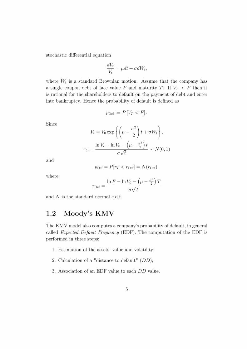
stochastic differential equation

dVt

Vt

= µdt+ σdWt,

where Wt is a standard Brownian motion. Assume that the company hasa single coupon debt of face value F and maturity T . If VT < F then itis rational for the shareholders to default on the payment of debt and enterinto bankruptcy. Hence the probability of default is defined as

pDef := P [VT < F ] .

Since

Vt = V0 exp

{(µ− σ2

2

)t+ σWt

},

rt :=lnVt − lnV0 −

(µ− σ2

2

)t

σ√t

∼ N(0, 1)

andpDef = P [rT < rDef] = N(rDef),

where

rDef =lnF − lnV0 −

(µ− σ2

2

)T

σ√T

and N is the standard normal c.d.f.

1.2 Moody’s KMV

The KMV model also computes a company’s probability of default, in generalcalled Expected Default Frequency (EDF). The computation of the EDF isperformed in three steps:

1. Estimation of the assets’ value and volatility;

2. Calculation of a "distance to default" (DD);

3. Association of an EDF value to each DD value.

5

The original KMV module is based on the Merton Model and

DD0 = −rDef.

In general,

DDt =lnVt − lnF +

(µ− σ2

2

)τ

σ√τ

(1.1)

where τ = T − t. Step 3 of the KMV model associates an empirically calcu-lated default frequency to a DD value. At this moment they use a data basewith over 250.000 company years and over 4.700 defaults (see [Dwyer et all]or [Crosbie et all]).

The computation of the EDF is performed in the following way:

• We assume that the DD takes values in some fixed interval, for instance[−20, 20]. We divide this interval into subintervals of a fixed length, forinstance 0.1

• We compute for each interval I how many times the DD takes valuein the interval.

• We compute for each interval I how many times the DD takes value inthe interval and the company defaulted during the next twelve months.

• The EDF is the quotient of the two previous values. It associates aprobability of default during the next twelve months to a DD.

Since 2006 Moody’s KMV model computes the DD in a different way,assuming the Vasiceck-Kealhofer model. That will not be relevant to whatfollows.

We remark that the association of a probability of default to a DD de-pends on the time horizon we are choosing. It is quite different to predict thatfor a certain DD value the company in question will default in six monthsor in eighteen months.

6

1.3 DD and Bank Defaults

The financial sector has an essential role in the economy as it is the mainprovider of funds to companies for investing and expanding its business.The 2008 financial crisis provided a stark reminder of what happens whenuncertainty and insolvency grip major financial corporations, the viability ofthe entire economy is put into question, as the credit flows dry up.

Since the crisis, financial stability has become an even greater concern forcentral banks and international financial overseers around the world. In fact,numerous central banks, the International Monetary Fund and the WorldBank have started publishing financial stability reports. For many years rat-ing agencies were the main agents for ascertaining the stability of institutions.Recently, their prominent role has been increasingly questioned from variouspolitical and economic quadrants, including the governments of developedworld countries.

Chan-Lau and Sy remark that among the quantitative tools used for as-sessing financial stability, an increasing number of central banks and inter-national financial institutions are encouraging the use of market based riskmeasures for banks and non-financial corporates [Chan-Lau et all].

Wong, Hui and Lo assess whether agency ratings and market-based de-fault risk measures are consistent for East Asian banks during the periodfrom 1996 to 2006: While the market-based measures are broadly consistentwith the credit rating assessments for the banks in the developed economies,the discrepancy between ratings and the market-based measures for the EastAsian banks are significant. The credit ratings had been adjusted slowly forthe East Asian banks during the onset of the Asian financial crisis. The rel-atively higher default risk implied by ratings during the post-crisis period ispartly due to the conservatism of rating agencies and the unsolicited ratings[Wong et all].

Among these market based risk measures the distance to default is cer-tainly the most interesting one. Several papers use a distance to defaultbased on the Merton model to assess the probability of default:

• Carlson, King and Lewis [Carlson et all] develop an index of finan-cial sector health using Merton’s DD. Their index spans over three

7

decades and captures periods when financial sector institutions werestrong and when they were weak. Using vector auto-regressions theyassess whether other indexes of financial-sector health affect the realeconomy, in particular non-residential investment. Three decades ofresults show that their index has a considerable impact.

• Pereira and Rua [Pereira et all] propose a linear factor pricing modelthat includes a bank risk factor, in addition to the standard marketrisk factor. The aggregate bank risk factor is defined as the change inthe average distance to default across all banks.

We will now test the distance to default’s efficiency at diagnosing a com-pany’s default, using ROC analysis.

8

Chapter 2

ROC Analysis

2.1 ROC curve

We want to develop a methodology to estimate the quality of a diagnosticmodel. In our case the topic is to ascertain from the variation or the valueof the Distance to Default the likelihood of a corporation defaulting on itsdebt obligations during a subsequent time period. We may consider severaldifferent diagnostic models for month m. The simplest approach would beto compare the value of the DD in month m with a chosen threshold t. Amore complex approach would be to compare the value at m of a function F

of the DD with t. F could be, for instance:

• the 6 month moving average of the DD;

• the function that associates the number DD(m)−DD(m− 6) to m.

Lets say that the function F is the diagnostic model for the DD. Letsestablish a threshold t. We will predict the likelihood of a default occurringover the next say 12 months if DD(m) < t. At first it is not obvious whichis the best value for t. We may test for various values of t. By looking at theROC curve being generated we may test for every value of t simultaneouslyand determine whether or not the model is producing good results. Whendoing this we also obtain what the best choice for the value of the threshold t

is, depending on the diagnostic errors we deem most important to minimize.

9

ROC means receiver operating characteristic, a terminology that comesfrom signal detection theory. For more a more detailed introduction to ROCanalysis, see [Metz] or [Fawcett].

When we are building a diagnostic model of this kind there are fourpossible classifications for our test values’ outcome:

• True Positive (TP ): we diagnose a default and it occurs;

• True negative (TN): we do not diagnose a default and it does notoccur;

• False Positive (FP ): we diagnose a default and it does not occur;

• False Negative (FN): we do not diagnose a default and it occurs.

Let us consider a set of 5000 corporations and a time span from January 1964to December 2012. We know the DD values for at least a significant part ofthe time interval specified above. We will set a threshold DD value, t. Givena company C and a month m with a corresponding DD value, according toour model one of the four already mentioned possibilities will occur. We willregister the number of TP ’s, TN ’s, FP ’s and FN ’s. We will thus obtainTP (t), TN(t), FP (t) and FN(t). We shall define true positive rate (TPR)and true negative rate (TNR) as:

TPR =TP

TP + FN, FPR =

FP

FP + TN.

We will now construct a curve in the ROC space, where FPR and TPR aredefined as the x and y axes respectively. Strictly speaking, the ROC spaceis the square [0, 1]× [0, 1]. We fix a set {t0, t1, ..., tn, tn+1} of thresholds with

t0 = −∞, t1 < t2 < · · · < tn, tn+1 = +∞.

We conventioned that FPR(−∞) = TPR(−∞) = 1, TPR(+∞) = FPR(+∞)

= 0. The ROC curve is obtained by associating to each threshold value t ofthe set {t0, ..., tn+1} the point (TPR(t), FPR(t)) and then joining the pointsby interpolation in order to obtain a curve.

The continuous line of 3.1 is a typical example of a ROC curve.

10

2.2 Area of the ROC curve

Suppose that we have a perfect predictive model. This means that for somevalue of s0 we will not have any false positives or negatives. Hence

FP (s0) = FN(s0) = 0.

ThereforeFPR(s0) = 0, TPR(s0) = 1.

The ROC curve associated to this perfect predictive method would be theone presented in figure 2.1.

6

-

TPR

FPR

t

t1

1Figure 2.1: Best possible ROC curve

The area of the set below the ROC curve would be 1.Now lets suppose we have a predictive model that always fails. This mean

that for each value of t we will not have any true positives or true negatives.Hence

TP (t) = TN(t) = 0.

ThereforeFPR(t) = 1, TPR(t) = 0.

The ROC curve associated with this predictive method would be the onepresented in figure 2.2.

The area of the set below the ROC curve would be 0.

11

6

-

TPR

FPR

s

s1

1

Figure 2.2: Worst possible ROC curve

The examples above show that it makes some sense to assume that thearea below the ROC curve measures the quality of the predictive method.With area=1 we have a perfect method. With area=0 we have a totallydefective method. With area=0.5 we have a method equivalent to flipping acoin. Empirical studies show that an area close to 0.8 indicates a significantlyrobust predictive model (see [Fawcett]).

A good ROC curve, like the one in figure 2.3, is always above the diagonalline and as close as possible to the best possible ROC curve (see figure 2.1).

How to calculate the area below the ROC curve on the left side of figure2.4?

Its area is the sum of the areas of the geometric figures on the right handside of figure 2.4. We remark that the area of the quadrilaterum on the righthand side of figure 2.4 equals

ab+ c

2.

12

6

-

TPR

FPR

s

s1

1����

����

I

AAK

�

�������

Figure 2.3: A good ROC curve

After marking the points associated to each threshold in the ROC spacethere are two ways to define a ROC curve. We can interpolate these points.This was our choice. The alternative choice is to connect a point with thepoint immediately to its right drawing first an horizontal line and after avertical line. This second choice seems to have several advantages from atheoretical point of view. When the data are very large the two ROC curves

13

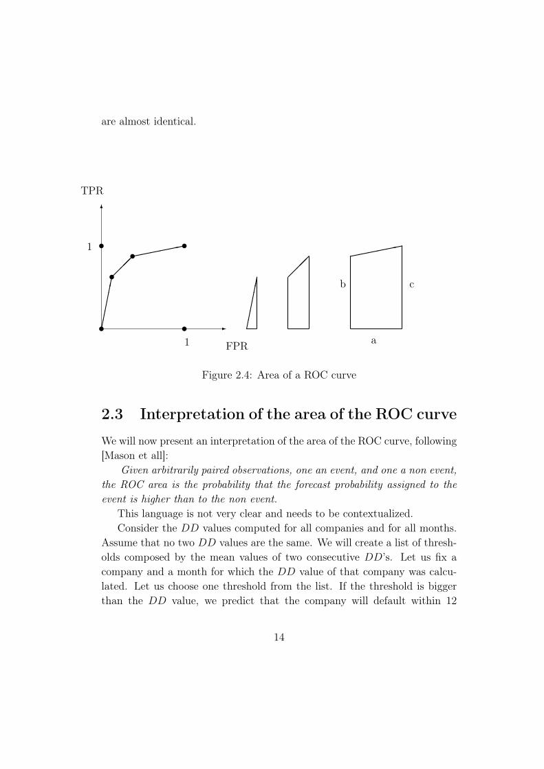
are almost identical.

6

-

TPR

FPR

t

t1

1t

tt t

���������

������

���

a

b c

Figure 2.4: Area of a ROC curve

2.3 Interpretation of the area of the ROC curve

We will now present an interpretation of the area of the ROC curve, following[Mason et all]:

Given arbitrarily paired observations, one an event, and one a non event,the ROC area is the probability that the forecast probability assigned to theevent is higher than to the non event.

This language is not very clear and needs to be contextualized.Consider the DD values computed for all companies and for all months.

Assume that no two DD values are the same. We will create a list of thresh-olds composed by the mean values of two consecutive DD’s. Let us fix acompany and a month for which the DD value of that company was calcu-lated. Let us choose one threshold from the list. If the threshold is biggerthan the DD value, we predict that the company will default within 12

14

months. Otherwise we will predict there will be no problems within the next12 months. The probability that we forecast default equals the ratio of thenumber of thresholds above the DD value by the number of all thresholds.The probability that we forecast there is no default equals the ratio of thenumber of thresholds below the DD value by the number of all thresholds.

If the default occurred, the sentence the forecast probability assigned tothe event is higher than to the non event ( for a certain company, at a certainmonth ) means that there are more thresholds above the DD value computedfor that company, that month, than below that DD value (if we take an arbi-trary threshold from the list, the probability that the diagnostic associated tothis threshold is correct is bigger then the probability that it is not correct).If there was no default, the sentence means that there are more thresholdsbelow the DD value than above.

The sentence arbitrarily paired observations, one an event, and one a nonevent means the two possibilites that can occur to a company twelve monthsafter we computed its DD. The event means what happened, default or nodefault; the non event, the other possibility.

We can look at this process of diagnostic in the following way: eachthreshold "has a vote". The thresholds above the DD value vote for the pre-diction of default. The thresholds below the DD value vote for the predictionof non default.

We can now give a first interpretation of the sentence of [Mason et all]:If we choose at random a company and a month for each the DD of that

company was computed, the probability that there are more votes for thanvotes against the correct prediction equals the area of the ROC curve.

If we consider the voting procedure as a decision procedure we obtain asimpler interpretation:

The probability that a prediction is correct equals the area of the ROCcurve.

We remark that this decision procedure is equivalent to diagnosing thedefault using as threshold the median of all the DD values considered.

We consider this huge set of thresholds in order to provide a theoreticalinterpretation of the ROC curve area. When we just want to compute theROC curve or its area we can consider a much smaller set of thresholds. We

15

compute the ROC curve using a grid of thresholds of the type T = m + ih,i = 1, ..., k, with m ≤ −10, m+kh ≥ 10 and h small enough we obtain a verysimilar value for the area of the ROC curve. We set h = 0.3 and k = 100.

16

Chapter 3

Data Analysis

3.1 Data Portfolios

I was given access to files with distance to default data on 225 financial com-panies and 5561 non-financial companies, identified by their permno’s (theseare the data used in [Pereira et all]) and several files on default data. Thedata we used took into account not just standard bank defaults but also de-fault announcements, bankruptcy fillings announcements and other defaultrelated events. These files originated from S&P, Moody’s and Bloomberg.They included dates of default of companies identified by name or by theCUSIP identification code. The files include the financial companies tradingon the NYSE, AMEX and NASDAQ stock exchanges with SIC codes be-tween 6020 and 6036. This includes the commercial banks and other savinginstitutions. It excludes bank holding companies (SIC code 6712) becausethey can have non bank subsidiaries. Investment banks, Security Brokers,Dealers, Exchanges and similar financial companies (SIC codes 6200 to 6299)are also excluded because lending is not their main activity (see [Pereira etall]).

The first task I had to handle was to cross all this data, producing a filethat included an identification of the company, a default date, if the companyever defaulted, and the DD data. This was one of the biggest challenges of thethesis. Sometimes the crossing was handled manually, others using MatLabroutines. A small part of the data had to be eliminated because there were

17

problems in the data crossings. For instance, we could not obtain the CUSIPnumber from the permno.

Another problem was how to handle the defaults. If a company defaultsseveral times in close succession and the waiting time between two defaults isalways less than one year, it seems clear that we should consider only the firstone. The fact that a company defaulted less than a year ago is much moresignificant than any DD data. What to do if a company stops defaulting forfive years and than defaults again? These cases were not considered becausethey were very few and there would be no significant gain in including them.

The file on financial companies includes 225 companies, 13 of each de-faulted in the period for which the DD data were computed. On averagethere are about 73 DD data each month. The average DD one year beforedefault, if it occurred, is equal to −0.9155. The average value of the DD

equals 1.3292.The file on non-financial companies includes 5381 companies, 78 of each

defaulted in the period for which the DD data were computed. On averagethere are about 1754 DD data each month. The average DD one year beforedefault, if it occurred, is equal to 0.982. The average value of the DD equals4.4141.

Both files include data from the period May 1963 - July 2012.The difference between the average DD values of financial and non finan-

cial companies reinforces the intuitive idea that a bank is a very specific typeof company.

We use the DD estimates of Pereira and Rua [Pereira et all]. We recallhow they were obtained. The market value of a company’s equity can be seenas a call option on the value of the company’s assets with maturity T andstrike price F equal to the value of the debt. By the Black-Scholes formula

St = VtN(d1)− Fe−iτN(d2) (3.1)

where i is the risk free interest rate,

d1 =ln(Vt/F ) + (i+ σ2/2)τ

σ√τ

, d2 = d1 − σ√τ and τ = T − t.

They follow the iterative procedure of Vassalou and Xing [Vassalou et all],which is similar to the Moody’s procedure (see Dwyer and Qu [Dwyer et all]):

18

• to use daily stock returns to compute the volatility of the equity;

• to use the volatility of the equity as a starting value for the volatilityσ of the assets;

• to solve (3.1) each day, assuming F to be the total debt of the bankand that the total debt is due in a year;

• use the daily series for Vt obtained in this way to obtain a better esti-mate of σ;

• go back to the second step and repeat the procedure until the differenceof two consecutive estimates of σ is less than 10−4;

• the final series of Vt is used to estimate the mean value of µ.

3.2 DD and Default

We computed the ROC curves and ROC curve areas of the DD’s of the banksand other non financial companies on our portfolios, using the algorithmdescribed in section 1 of Appendix A. The time horizon considered is oneyear. If the DD of a bank goes below the threshold, is is predicted that thebank will default before one year is passed. The ROC curves are presentedin figure 3.1.

Its areas are presented in table 3.1.

Banks Non FinAreas 0.7878 0.845

Table 3.1: ROC curve areas

19

0 0.2 0.4 0.6 0.8 10

0.1

0.2

0.3

0.4

0.5

0.6

0.7

0.8

0.9

1

FPR

TP

R

Banks

Non−Fin

Figure 3.1: ROC curves - Banks and Non financial

The results are more or less what we expected:

• The model’s ROC curve area for the non-financial company portfoliohas a high value. It shows that the use of the DD model with athreshold value is a robust technique for measuring the financial solidityof a company.

• The model’s ROC curve area for the financial companies is still highenough to be trusted, but lower than the other area. The reasons forthis difference are well known: it is quite dangerous to let a bank de-fault because of its systemic consequences. Thus, financial company de-faults are usually avoided, traditionally through a government arrangedmerger or takeover of the troubled institution by a bigger bank. Nowa-days, straight government bailouts have been often employed, generat-ing controversy due to the possible moral hazard implications.

20

3.3 Data Analysis

To collect data in the real world is not easy. One of the questions someonedoing this type of work keeps asking is: did my model catch all the defaults?Since the number of defaults is quite small when compared with the numberof companies, to miss a few defaults is enough to change significantly theresults obtained.

Algorithm 1 of Appendix A takes note of the percentage of false positivesthat the model generates. Figure 3.2 shows the percentage of false positivesfor each bank relatively to all the thresholds considered.

Figure 3.2: False Positive ratio - Banks

The eight banks with more than 60% of false positives were checked. Wecould not find any reference on the internet to a default by any of thesebanks. Hence we can say that our data base is quite accurate. We remarkthat four of these eight banks merged with a bigger bank within two yearsof its sharp DD decrease, which points to the existence of serious financialdistress, which the DD value variation captured.

Note that we do not count bank mergers as defaults. However, in manycases these mergers are preventive "forced" actions to avoid default. Hence,our ROC area actually underestimastes the predictive ability of the DD forbanks.

21

It may seem odd that the average percentage of false positives is about50%. We should notice that the algorithm runs over a wide range of thresh-olds. When the threshold is high almost all the results are false positives.In order to get a more accurate estimate of the ROC curve area we shouldconsider all types of thresholds.

3.4 Case Studies

We present three case studies. The first one is a textbook one, where thedefault warning arrives in due time. In the second case the DD has a hugedecrease but it is not the first warning sign. We explain why this cannotbe considered a flaw of the method we are testing. In the third case wepresent the example of a false positive. Although there was no default theDD decrease provided a warning about the bank’s financial troubles thatended in a hostile takeover by a much smaller bank.

3.4.1 The Continental Illinois Bank

Before its collapse the Continental Illinois (permno 57250) was the seventhlargest bank in the United States. It became insolvent in 1984 due to a cor-ruption scandal in which the management approved very risky loans [Singer],[Zweig]. The term "too big to fail" was popularized in a 1984 Congressionalhearing, discussing the Federal Reserve and Federal Deposit Insurance Cor-poration’s (FDIC) intervention with Continental Illinois [New York Times].

The graph of figure 3.3 includes two vertical lines. The second one marksthe date of the first default. The first one marks the date when the DD issupposed to give a warning sign that the bank is in risk of default, one yearbefore the date of default.

22

75 80 85−12

−10

−8

−6

−4

−2

0

2

4

Years

DD

Figure 3.3: Continental Illinois Bank

The FDIC infused 4.5 billion dollars to rescue the bank, preventing theloss of virtually all deposit accounts and even bondholders. The FederalGovernment intervened, with a 5.5 billion dollars of new capital bailout and8 billion dollars in emergency loans. These measures did not prevent a sub-stantial run on the bank’s deposits that ended in a default.

The percentage of banks with a DD lower than Continental Illinois 1 yearbefore the default was 2.78%.

3.4.2 Citizens Republic Bancorp

In 2008, the Citizens Republic (permno 86685) took a 300 million dollarsTroubled Asset Relief (TARP) loan to survive the economic downturn. Itstroubles are reflected by the decrease in the DD, which gets close to −2 oneyear before the default. In 2010, Citizens Republic sold its F&M Bank Iowalocations for 50 million dollars to Great Western Bank. This measure had apositive effect on the DD value.

23

1990 1995 2000 2005 2010 2015−8

−6

−4

−2

0

2

4

6

8

Figure 3.4: Citizens Republic Bancorp

For the first time since the economic downturn, the Bank reports in July2012 five consecutive quarters of profit [Flint Journal]. This development isalso reflected in the evolution of the DD.

The percentage of banks with a DD lower than Citizens Bancorp 1 yearbefore the default equals 10.6%. Two months later this percentage decreasedto 4.3%.

3.4.3 The NatWest

The NatWest (officially named National Westminster Bank, permno 70885)was the largest retail and commercial bank in the United Kingdom.

24

1992 1993 1994 1995 1996 1997 1998 1999 2000 2001−8

−7

−6

−5

−4

−3

−2

−1

Figure 3.5: Nat West Bank

In 1997, NatWest Markets, the corporate and investment banking arm ofNat West announced a £90.5m loss due to the poor management of complexderivative products, which was already reflected in the huge decrease of thebank’s DD. The DD recovered due to the selling of several subsidiaries,including the toxic ones. From that moment on the bank was considered atarget for hostile takeover bids. Partially in order to escape that fate the NatWest Bank announced a merger with the insurance company Legal & Generalin a friendly 10.7 billion pounds deal. The move received a poor receptionin the financial markets. Its market value and its DD had another steepdecrease. These developments encouraged the Royal Bank of Scotland to tryan initial hostile takeover, which was rejected. It succeeded in its second trysometime later [Guardian 99], [Guardian 99b]. Nat West, once Britain’s mostprofitable bank, was delisted from the London Stock exchange, becoming asubsidiary of the Royal Bank of Scotland.

Twelve months before attaining its lowest DD in the period consideredin the graph, NatWest had a DD of −1.8217. Only 2.08% of the banks hadlower DD at this month.

25

Chapter 4

Alternative Default DiagnosticMethods

4.1 Moving Averages

It is quite common to use moving averages in order to smooth out time seriesand decrease the importance of outliers. To consider a time series wouldshorten the ideal time horizon of our diagnostic method. On the other handthere was a possibility that this procedure would eliminate false positives,due to the smoothing out effect. Figure 4.1 plots the areas of the ROC curvesobtained when the lag L of the moving average of the DD goes from 1 to 12.

Lag Time Horizon (months) ROC area1 12 0.78692 11 0.78763 11 0.78374 10 0.7855

Table 4.1: ROC curve areas

26

0 2 4 6 8 10 120.72

0.73

0.74

0.75

0.76

0.77

0.78

0.79

0.8

Lag

Are

a

Figure 4.1: ROC Areas Moving Averages - Banks

The best performance of the diagnostic method is obtained when the lagequals 2. Table 4.1 describes some of the areas obtained in the case plottedin figure 4.1. A minimal smoothing (a lag of two) produces slightly betterresults. Is this a random fluctuation or something more substantial?

The analysis of the Non Financial companies portfolio suggests that it isindeed only a random fluctuation (see figure 4.2).

27

0 2 4 6 8 10 120.805

0.81

0.815

0.82

0.825

0.83

0.835

0.84

0.845

0.85

0.855

Lag

Are

a

Figure 4.2: ROC Areas Moving Averages - Non Fin.

4.2 Steep descents

We tried to detect defaults by looking at steep decreases in the value of theDD. The ROC analysis did not produce the expected results.

28

Conclusions

We performed a ROC analysis of the default diagnostic method based on theDistance to Default associated to the Merton Model. This analysis showedthat this Distance to Default provides a reliable warning that a bank candefault on the time horizon of one year. The ROC analysis shows thatthe results are not as good as the ones obtained with non financial firms,but nevertheless, robust. It seems reasonable to assume that this differencein performance results essentially from the fact that, due to the problemscreated by a bank default, there is a tendency for a last moment bailout ormerger of the bank that allows it to avoid default.

We concluded also that the diagnostic model provides the best possibleresults when we consider a time horizon of one year. Moreover, a smoothingof the DD data, that could potentially eliminate many false positives, didnot improve the diagnostic performance.

29

Appendix A

Matlab Programs

A.1 Main Algorithm

The main objective of this algorithm is to associate a ROC curve to a set ofdata that contains the eventual first default date of a company, its permnoand the monthly distance of default of that company on some time intervalthat starts after December 1963 and ends before January 2013.

If one considers also the steps marked with an asterisk we will associateto each company a percentage of false positives. A much higher than averagepercentage of false positives indicates the possibility of the existence of adefault that was not detected. This is a good way to improve the quality ofthe data.

We will number the months starting from January 1964.

1. We will have the following inputs:

(a) the number ncompany of companies listed ;

(b) the number of months nmonth considered in the study;

(c) the number of thresholds nthreshold we intend to consider;

(d) the length delay of the time interval where we expect the previsionof default should occur (in months);

(e) An ncompany×(nmonth+2) data Matrix where the first line con-tains the company’s permno and the second line the number of

30

the month when the company defaulted, if that is the case. Theremaining lines contain the company’s DD’s, ordered by month.

2. We create four ncompany×1 matrices that will register the number ofTP, TN, FP and FN that will occur for each company in each month,for all the thresholds considered (see chapter 2).

3.∗ We create an ncompany×1 matrix FFP. The first line will register thepermno of companies. The fourth line will register the number of falsepositives that occur for each company and over all thresholds and allmonths. The third line will register the number of months for whichthere are DD computed for each company. Moreover,

FFP (2, i) = FFP (4, i)/FFP (3, i), for each i.

4. We will start three cycles. The first generates all the thresholds weintend to consider. The number of thresholds must be big enough sothat each point of the ROC curve is close enough to the next one. Theremust exist thresholds big enough and small enough so that there arepoints of the ROC curve close enough to (0, 0) and (1, 1). The secondcycle runs over the companies. The third cycle runs over the months.

5. For each value t of the threshold, each company and each month suchthat the company has a DD, one of the numbers TP (t), TN(t), FP (t),FN(t) increases by a unit, according with the fact that the diagnosticof the model we are using was a true positive, a true negative, a falsepositive or a false negative.

This step and the next one are the only ones that depend on the diag-nostic method we have chosen.

6.∗ At the same time we count the number of false positives that occur foreach company.

7. We close the three cycles initiated above.

8. We compute for each threshold the values FPR and TPR and draw theROC curve. We calculate the area of the ROC curve.

31

A.2 Variations on the ROC curve algorithm

• In section 4.1 we introduce an external cycle in the main program thatruns over a set of lags, replacing in each column of the data matrix theDD series by a convenient moving average with a given lag, recordingthe ROC curve areas obtained for each lag. Finally, it produces agraphic of the variation of the ROC curve area.

• In section 4.2 we change the criteria for true positives, false positivesand so on and introduce an external cycle that runs over a set of lags.Each lag determines a distance between the first and the second readingof the DD that are compared to decide if it occurred a big decreasein the DD. Finally, it produces a graphic of the variation of the ROCcurve area.

32

Appendix B

Files

We worked with the following data:

• A file with data on DD of 1408 banks, identified by permno:

bank_pd_NYSE-AMEX-NASDAQ_20130712_FULL

• Four files with data on DD of non financial companies, also identifiedby permno:

bank_pd_ONLY_NONFIN_NYSE-AMEX_20130716_FULL_1bank_pd_ONLY_NONFIN_NYSE-AMEX_20130716_FULL_2bank_pd_ONLY_NONFIN_NYSE-AMEX_20130716_FULL_3bank_pd_ONLY_NONFIN_NYSE-AMEX_20130716_FULL_4

Several Excel and Access files containing data on Defaults and a masterfile with names of companies and two code identifiers: CUSIP and permno.We had to cross the data. In some cases the Defaults were only identifiedby names of companies and we had to obtain their permno’s. We had tocreate several MATLAB programs to change the names into CUSIP’s and theCUSIP’s into permno. In two cases the names were not written in differentfiles using the same conventions and the matching had to be done by hand.This matching process took about half of the working time of this thesis.

• At the end of this process we obtained the files:

33

DDBanksDDNF

The first lines of these files contain the permno identifiers. The secondones contain the month of the first default, if there is one, or the number1000 otherwise . The months are numbered from January 1964. The otherlines contain the DD of each month.

34

List of Figures

2.1 Best possible ROC curve . . . . . . . . . . . . . . . . . . . . . 112.2 Worst possible ROC curve . . . . . . . . . . . . . . . . . . . . 122.3 A good ROC curve . . . . . . . . . . . . . . . . . . . . . . . . 132.4 Area of a ROC curve . . . . . . . . . . . . . . . . . . . . . . . 14

3.1 ROC curves - Banks and Non financial . . . . . . . . . . . . . 203.2 False Positive ratio - Banks . . . . . . . . . . . . . . . . . . . 213.3 Continental Illinois Bank . . . . . . . . . . . . . . . . . . . . . 233.4 Citizens Republic Bancorp . . . . . . . . . . . . . . . . . . . . 243.5 Nat West Bank . . . . . . . . . . . . . . . . . . . . . . . . . . 25

4.1 ROC Areas Moving Averages - Banks . . . . . . . . . . . . . . 274.2 ROC Areas Moving Averages - Non Fin. . . . . . . . . . . . . 28

35

Bibliography

Carlson et all M. Carlson, T. King and K. Lewis, Distress in the FinancialSector and Economic Activity 1, Board of Governors of the FederalReserve, Washington, DC.

Chan-Lau et all J. A. Chan-Lau and A. N.R. Sy, Distance-to-default inbanking: A bridge too far?, Working Paper No. 06/215, InternationalMonetary Fund (2006).

Costa G. Ferreira da Costa, Alternative Models to approximate Moody’sDistance to Default, Master Thesis in Financial Mathematics, ISCTE-DMFCUL, oriented by Professor João Pedro Pereira, (2011).

Crosbie et all P. Crosbie and J. Bohn, Modeling defaul risk, Moody’s KMV.

Dwyer et all D. Dwyer and S. Qu, EDF 8.0 Model Enhancements, Moody’sKMV.

Fawcett T. Fawcett, ROC Analysis in Pattern Recognition, Pattern Recog-nition Letters Volume 27, Issue 8, June 2006, Pages 882−891.

Goodhart et all C. Goodhart, P. Sunirand and D. Tsomocos, A risk as-sessment model for Banks, Annals of Finance, 1, Pag 197−224, (2005).

Green et all D. Green and J. Sweets, Signal detection and Psycophysics,Peninsula Publishing, Los Altos, California, USA.

Hull et all John C. Hull, I. Nelken and A. D. White, Merton’s model, creditrisk and volatility skews, Journal of Credit Risk, Volume 1, Issue 1,Winter 2004/2005, Pages 3−27.

36

Mason et all J. Mason, N. Graham, and E Nicholas Areas beneath therelative operating characteristics (ROC) and relative operating levels(ROL) curves: Statistical significance and interpretation, QuarterlyJournal of the Royal Meteorological Society (128): 2145−2166 (2002).

Merton R. C. Merton, On the Pricing of Corporate Debt: the Risk Structureof Interest Rates, Journal of Finance 28, 1974, Pages 449−470.

Metz C. E. Metz, Basic principles of ROC analysis, Seminars in NuclearMedicine Volume 8, Issue 4, October 1978, Pages 283−298.

Munves et all D.W. Munves, A. Smith and D.T. Hamilton, Banks andtheir EDF Measures Now and through the Credit Crisis: Too High, TooLow or Just About Right?, Moody’s Capital Market Research, ReportNumber 129462.

Pereira J. P. Pereira, Credit Risk, Teaching notes, ISCTE-IUL.

Pereira et all J. P. Pereira and A. Rua, Asset Pricing with a bank riskfactor, working paper ssrn.1975249.

Singer M. Singer, Funny Money, New York: Knopf, 1985.

Vassalou et all M. Vassalou and Y. Xing, Default risk in equity returns,Journal of Finance, 59(2), 831−868.

Vasicek O. A. Vasicek, Credit Valuation, KMV company.

Wong et all T. C. Wong, C. H. Hui and C. F. Lo, Ratings Versus Market-Based Measures of Default Risk of East Asian Banks, 20th AustralasianFinance & Banking Conference 2007 Paper.

Zweig P. Zweig, Belly Up: The Collapse of the Penn Square Bank, NewYork, Crown, 1985.

European Comunity The Economic Adjustment Programme for Cyprus,EUROPEAN ECONOMY, Occasional Papers 149, May 2013, The Eu-ropean Comunity, Directorate-General for Economic and Financial Af-fairs.

37

Flint Journal Citizens Republic Bancorp Inc. plans to sell Iowa subsidiaryfor $50 million cash and Citizens Republic Bancorp part of lumber,automotive, Flint history since 1871, The Flint Journal, February 1,2010 and September 13, 2012.

Guardian 99 L. Buckingham, J. Treanor and L. Laird, NatWest pounceson L&G with £11bn takeover bid, The Guardian, 03.09.1999.

Guardian 99b NatWest rejects takeover bid, The Guardian, 24.04.1999.

New York Times E. Dash, If It’s Too Big to Fail, Is It Too Big to Exist?,The New York Times 21.06.2009.

38