RICARDO FEYH RIBEIRO - UFRGS

MINISTRY OF EDUCATION

FEDERAL UNIVERSITY OF RIO GRANDE DO SUL

School of Engineering

Post-graduation Program in Mining, Metallurgy and Materials

PPGE3M

ANNULUS CO2-CORROSION OF HIGH STRENGTH STEEL WIRES FROM

UNBOUNDED FLEXIBLE PIPES

(Corrosão por CO2 de arames de aço de alta resistência mecânica provenientes de dutos flexíveis de

camadas não aderentes)

RICARDO FEYH RIBEIRO

Thesis submitted for the degree of Doctor of Philosophy in Engineering.

Porto Alegre

June 2019


Annulus CO2-corrosion of high strength steel wires from unbounded flexible pipes

A study conducted at the Department of Metallurgy

from School of Engineering of UFRGS within the

Graduate Program in Mining, Metallurgy and

Materials - PPGE3M, as part of the requirements for

obtaining the title of Doctor of Philosophy in

Engineering.

Concentration Area: Science and Technology of

Materials

Advisor: Prof. Dr. Carlos E. F. Kwietniewski

Porto Alegre

June 2019

II


Corrosão por CO2 de arames de aço de alta resistência mecânica provenientes de dutos

flexíveis de camadas não aderentes

Trabalho realizado no Departamento de Metalurgia da

Escola de Engenharia da UFRGS, dentro do Programa

de Pós-Graduação em Engenharia de Minas,

Metalúrgica e de Materiais –PPGE3M, como parte dos

requisitos para obtenção do título de Doutor em

Engenharia.

Área de Concentração: Ciência e Tecnologia dos

Materiais

Advisor: Prof. Dr. Carlos E. F. Kwietniewski

Porto Alegre

Junho 2019

III


Annulus CO2-corrosion of high strength steel wires from unbounded flexible pipes

This dissertation was deemed adequate to obtain a

PhD degree in Engineering, area of concentration

in Science and Technology of Materials, and

approved in its final form, by the advisor and by

the examining board of the Postgraduate Program.

A

Advisor: Prof. PhD. Carlos Eduardo Fortis Kwietniewski

A

Coordinator of PPGE3M: Prof. Dr. Carlos Pérez Bergmann

Examining board:

Prof. Dr. André Ronaldo Froehlich, UNISINOS

Prof. Dra. Cristiane Pontes de Oliveira, UFRGS

Prof. Dr. Tiago Falcade Nunes, UFRGS

IV

Eu dedico esta dissertação a meus familiares, a

minha esposa e a meus amigos.

V

ACKNOWLEDGEMENTS

Many people have generously contributed with their time and knowledge to the

development of this work, making it a tough task to list all who deserve recognition. However,

some of the major contributors and their affiliations are as follows:

To Prof. PhD Carlos Eduardo Fortis Kwietniewski for offering me advisory and

extensive support and friendship throughout my career.

To John Rothwell, Shiladitya Paul and Lukas Suchomel, from The Welding Instute, that

deserve special recognition for their advisory, help and friendship. This work would certainly

not be possible if weren’t their involvements.

To Prof. PhD Afonso Reguly, Prof. PhD Thomas Clarke and Prof. PhD Telmo Roberto

Strohaecker (in memoriam) for offering opportunities to develop work in my area of expertise

in the Physical Metallurgy Laboratory (LAMEF).

To all of the members of BG Group/Shell, the Welding Institute (TWI) and LAMEF

who contributed to the development of this work or that made me feel welcome in the United

Kingdom. Allan Dias, Arnaud Tronche, David Seaman, Diego Juliano, Leury Pereira, Mariana

dos Reis Tagliari, Mike Bennett, Ricardo Baiotto, Nataly Araujo Cé, Richard Carrol, Rosane

Zagatti, Ryan Bellward, Sally Day, Sheila Stevens and all of the members of the group of

corrosion testing in aggressive environments (GECOR/LAMEF) deserve special recognition.

To my colleagues in the post-graduation program in Science and Technology of

Materials (PPGE3M).

To the national agency of oil & gas & biofuel, “Agência Nacional do Petróleo, Gás

Natural e Biocombustíveis (ANP)”, the Brazilian governmental agency “Conselho Nacional de

Desenvolvimento Científico e Tecnológico (CNPq)” and BG Group/Shell for sponsoring this

research through the Science Without Borders Program.

To my family, Andressa Wigner Brochier, Eng. Roberto Spinato Ribeiro, Stella Maria

Feyh Ribeiro, Fernando Feyh Ribeiro and Eng. Gustavo Feyh Ribeiro, for all of their love,

companionship and emotional support.

VI

ABSTRACT

Recent premature failures of unbounded flexible pipes brought life to the discussion of

the detrimental effects of the CO2 on the structural layers of unbounded flexible pipes. Flexibles

are structures composed of several concentric layers of polymers and steel wires. The steel

wires support the mechanical loads and reside inside a highly confined annulus space bounded

by two polymer layers. The environment in this occluded annulus region evolves as water and

other chemicals permeate from the produced fluid in the bore through the inner sheath, or from

breaches in the outer sheath. As a result, the armour wires can be subjected to corrosion that

needs to be considered against the service environment. The complexity of the annulus

environment makes the study of corrosion in it challenging. Thus, understanding the

interactions between the steel and the electrolyte is essential for reproducing the corrosion of

the structural layers. Despite that, many occluded CO2-corrosion tests are conducted in

environments, which neither reproduce the state of the electrolyte, nor the mechanisms found

in the field. Although some studies on corrosion in annulus environments have been published,

there remains further work to be done to fully understand the extent of variables that may

potentially affect the annulus corrosion rate and mechanisms within it, particularly concerning

the effect of CO2 permeation. The present study describes the corrosion rates of high strength

carbon steel wires in brines with carefully controlled supply rates. A simulation of the gas flow

rate was carried to study the permeation behaviour on severe CO2 service conditions. Weight

loss and electrochemical measurements were conducted to evaluate the corrosion rates.

Pressure, temperature and composition of the brine, covering liquid, gaseous and supercritical

states of CO2 have been explored by simulation in search for critical patterns. The data in low

pressure are compared to simulation and those of previous studies in the literature. The

experiments show low corrosion rates and a clear dependence between the concentration of

iron, pH, open circuit potential and corrosion rate. Changes in these properties were found to

describe three stages of corrosion. No substantial influence on the maximum corrosion rate was

seen after a two-fold increase in the CO2 supply rate.

Keywords: Unbounded flexible pipes; annulus CO2-corrosion; high strength steel; electrolyte

simulation.

VII

RESUMO

Recentes falhas prematuras de dutos flexíveis de camadas não aderentes trouxeram à

luz a necessidade de debater os efeitos prejudiciais do CO2 na deterioração das camadas

estruturais da tubulação. Estes tubos flexíveis são estruturas compostas por camadas

concêntricas de polímero e aço, nas quais as partes metálicas têm como objetivo suportar as

cargas mecânicas. As condições ambientais do interior do componente evoluem à medida que

água e outras espécies químicas adentram na região anular, que são provenientes do fluido

transportado, ou de rupturas na capa externa. Em consequência disto, as armaduras metálicas

podem estar sujeitas à corrosão. Assim, compreender as correlações entre as variáveis

ambientais com as propriedades do metal é vital para o entendimento do processo e da

reprodução do dano na estrutura. Porém, a complexidade do ambiente anular torna o estudo

desafiador. Por esta razão, muitos estudos encontrados na literatura foram conduzidos em

ambientes que não reproduzem o ambiente anular, nem os mecanismos observados em campo.

De fato, ainda há muito a ser feito para compreender o processo, particularmente no que diz

respeito ao efeito da permeação de CO2 na corrosão das armaduras de tensão. Neste aspecto, o

presente trabalho tem como objetivo descrever a corrosão dos arames de aço carbono de alta

resistência mecânica em solução contendo 3,5% de NaCl sob condições controladas de fluxo

de CO2. As simulações do fluxo de gás foram realizadas visando representar a permeação em

condições de serviço severo. As taxas de corrosão foram avaliadas por técnicas eletroquímicas

e de perda de massa. As variáveis do ambiente, pressão, temperatura e composição da solução,

foram explorados por simulações cobrindo os estados líquido, gasoso e supercrítico do CO2 em

busca de padrões críticos de corrosão. Os resultados obtidos nos experimentos foram

comparados com simulações e com dados encontrados na literatura. Os experimentos mostram

baixas taxas de corrosão e uma clara dependência entre a concentração de ferro, o pH, o

potencial de circuito aberto e as taxas de corrosão. Alterações nestas propriedades descrevem

três estágios. A taxa máxima de corrosão não foi significativamente afetada pelo aumento de

duas casas decimais no fluxo de gás.

Palavras chave: Dutos flexíveis de camadas não aderentes; Corrosão por CO2 do espaço

anular; Aço de alta resistência mecânica; Simulação do eletrólito.

VIII

FIGURES

Figure 1: Sketch of the lifetime attribution of flexible pipes. .................................................................................. 3 Figure 2: Norwegian statistics of the major incidents rate per riser operational year. ............................................. 4 Figure 3: Scheme of an unbonded flexible pipe structure. ...................................................................................... 6 Figure 4: Profile geometries of the pressure armour. a) Z-shape. b) C-shape. c) T-shape 1 with clip. d) T-shape. 7 Figure 5: End-fitting system. ................................................................................................................................... 8 Figure 6: Corrosion caused by a rupture of the outer sheath and ineffective cathodic protection. ........................ 12 Figure 7: Scheme of a bend limiter. ...................................................................................................................... 12 Figure 8: Bend restrictor. ....................................................................................................................................... 13 Figure 9: Subsea buoys connected to flexible pipes. ............................................................................................. 14 Figure 10: Five examples of riser configurations recommended by Standard API RP 17B. ................................. 15 Figure 11: General requirements for a corrosion process. ..................................................................................... 17 Figure 12: Free-energy diagrams. .......................................................................................................................... 20 Figure 13: Electrode reduction potentials of metals (VSCE), for seawater at 25 °C. The unshaded symbols show

ranges exhibited by stainless steels in acidic water, which could be related to occlusion and aeration aspects. ... 22 Figure 14: Fe-H2O Pourbaix diagram. ................................................................................................................... 23 Figure 15: Potential corrosion surfaces. ................................................................................................................ 24 Figure 16: Hypothetical scheme of a polarisation diagram. .................................................................................. 26 Figure 17: Polarisation curves of steel at different rotation rates. A test carried in brine solution saturated with

carbon dioxide at 20 °C. ........................................................................................................................................ 27 Figure 18: Schematic illustration of the permeation of gases from the bore into the annulus region. ................... 29 Figure 19: Five stages of the transport mechanism of a homogeneous non-porous polymer membrane at a given

temperature. ........................................................................................................................................................... 30 Figure 20: Effect of temperature on the solubility of carbon dioxide in water. ..................................................... 32 Figure 21: Effect of pressure on the solubility of carbon dioxide in water. .......................................................... 32 Figure 22: Phase diagram for carbon dioxide. ....................................................................................................... 33 Figure 23: Examples of variables that can affect the corrosion process of unbounded flexible pipes. ................. 36 Figure 24: Corrosion rate of a steel piling in seawater. ......................................................................................... 37 Figure 25: Annual average of the dissolved oxygen per depth. a) 0 metres. b) 1000 metres. c) 2000 metres. ...... 38 Figure 26: Images of the inner tensile layer of an unbonded flexible pipe. a) Shows the corroded wires without

the presence of the anti-wear tape and b) shows the anti-wear tape. ..................................................................... 39 Figure 27: Anodic polarisation curve of iron with the scan rate of 6.6 mV/s and rotating disk electrode at 69 rps

in 0.5 M Na2SO4 solution at pH5 and 25 °C. ......................................................................................................... 41 Figure 28: Effect of increasing pressure on the pH of the water/CO2 solution at 25 °C........................................ 43 Figure 29: The effect of pH in the absence of iron carbonate scales on measured and predicted corrosion rates.

Test conditions: 20 °C, pCO2 = 1 atm, 1 m/s, cFe2+ < 2 ppm. ................................................................................ 44

Figure 30: a) Effect of temperature on the corrosion of an API X65 steel at pH4 - LSV in 0.1M NaCl solution

with no CO2. b) Effect of pCO2 on the corrosion of an API X65 steel at pH4 - LSV in 0.1M NaCl solution at 30

°C........................................................................................................................................................................... 45 Figure 31: Crystal growth. ..................................................................................................................................... 47 Figure 32: Pourbaix diagrams for Fe-CO2-H2O systems at various temperatures (symbols: • - bulk pH, ° - surface

pH). a) 25 °C. b) 80 °C. c) 120 °C. d) 150 °C. ...................................................................................................... 48 Figure 33: Corrosion rate as a function of the V/S ratio. ....................................................................................... 51 Figure 34: Long-term evolution of pH measured in a confined test cell at ambient temperature, under 1 to 45 bar

(44,4 atm) of CO2. ................................................................................................................................................. 52 Figure 35: Corrosion rate as a function of the V/S ratio for different θ at pCO2 = 1 atm and 20 °C. ................... 53 Figure 36: pH as a function of the V/S ratio for different θ; at pCO2 = 1 atm and 20 °C. ..................................... 54 Figure 37: Annulus corrosion rate from weight loss measurements of specimens in CO2 saturated deionised

water at 50 °C. ....................................................................................................................................................... 54

IX

Figure 38: Localised corrosion on a specimen in CO2-saturated brine at 10 °C.................................................... 56 Figure 39: Organisational chart. ............................................................................................................................ 57 Figure 40: Main interactions between the system and the neighbourhood. a) Open carbonate system and b)

Closed carbonate system. ...................................................................................................................................... 60 Figure 41: a) Glass test vessel. b) Water sampling for iron ions. .......................................................................... 63 Figure 42: Scheme of the electrode layout for an electrochemical test in the occluded environment. The detail

shows the steel surface and the anti-corrosion lacquer used to define it. .............................................................. 64 Figure 43: Critical scaling tendencies at which protective corrosion scale begins to form in CO2-corrosion. ...... 68 Figure 44: Concentration of iron ions in the solution over time. The saturation with iron ions was simulated

under the environmental conditions tested in the laboratory. Test conditions: V/S of 0.2 ml/cm², 3.5%wt. NaCl

brine, FR/SS of 0.0008 ml.min-1.cm-2, 1 atm of CO2 and 30±2 °C. ...................................................................... 72 Figure 45: pH as a function of the iron concentration in the solution. Test conditions: V/S of 0.2 ml/cm², 3.5%wt.

NaCl brine, FR/SS of 0.0008 ml.min-1.cm-2, 1 atm of CO2 and 30±2 °C. ............................................................. 73 Figure 46: Simulation of a titration procedure for an open system composed of 3.5 %wt . NaCl solution saturated

with carbon dioxide at 30 °C and 1 atmosphere. The shadow indicates a range of pH typical from a flooded

annulus of unbounded flexible risers. .................................................................................................................... 74 Figure 47: Simulation of a titration procedure for a closed system composed of 3.5%wt. NaCl solution saturated

with carbon dioxide at 30 °C and 1 atmosphere. The shadow indicates a range of pH typical from a flooded

annulus of unbounded flexible risers. .................................................................................................................... 75 Figure 48: Comparison between open and closed carbonate systems. .................................................................. 76 Figure 49: Simulation of the composition of the brine as a function of the concentration of Fe2+. a) pH. b) HCO3

-.

c) CO32-. d) CO2(aq). e) FeCO3. The solution consists of 3.5%wt. NaCl brine saturated with carbon dioxide at 30

°C and 1 atmosphere. ............................................................................................................................................. 77 Figure 50: Simulation and experimental evolution of pH at 3.5% NaCl brine at 30 °C, 1 atm of CO2 and flow rate

of 0.0008 ml.min-1.cm-2. ........................................................................................................................................ 78 Figure 51: Evolution of the OCPs of working electrodes in the aqueous CO2 atmosphere at 30 °C and 1 atm,

with a FR/SS of 0.0008 ml.min-1.cm-2. .................................................................................................................. 79 Figure 52: Evolution of the measured and analytical OCP, iron concentration and pH. The plot shows 3 zones,

described by Roman numerals “I”, “II” and “III”. Test conditions: V/S of 0.2 ml/cm², 3.5%wt. NaCl brine,

FR/SS of 0.0008 ml.min-1.cm-2, 1 atm of CO2 and 30±2 °C. ................................................................................. 80 Figure 53: Simulation of [CO3

2-] inferred from the measured Fe2+. The modelled electrolyte consists of 3.5%wt.

NaCl brine saturated with carbon dioxide at 30 °C and 1 atmosphere. ................................................................. 81 Figure 54: Evolution of the LPR corrosion rate and polarisation resistance (Rp). Test conditions: V/S of 0.2

ml/cm², B of 36.7 mV/dec, 3.5%wt. NaCl brine, FR/SS of 0.0008 ml.min-1.cm-2, 1 atm of CO2 and 30±2 °C. .. 83 Figure 55: Evolution of the LPR corrosion rate, OCP, pH and Fe2+. Test conditions: V/S of 0.2 ml/cm², B of

36.7 mV/dec, 3.5%wt. NaCl brine, FR/SS of 0.0008 ml.min-1.cm-2, 1 atm of CO2 and 30±2 °C. ....................... 84 Figure 56: Plot of the linear sweep voltammetry at test end. Test conditions: 1 mV/s, V/S of 0.2 ml/cm²,

3.5%wt. NaCl brine, FR/SS of 0.0008 ml.min-1.cm-2, 1 atm of CO2 and 30±2 °C. ............................................... 86 Figure 57: Comparison of the corrosion rates obtained by LSV to results described in the literature at different

degrees of occlusion. ............................................................................................................................................. 87 Figure 58: Comparison of the corrosion rates to results described in the literature at different degrees of

occlusion. ............................................................................................................................................................... 89 Figure 59: Representative corrosion surface of the samples, demonstrating the specimens before and after the

test. Test conditions: V/S of 0.2 ml/cm², 3.5%wt. NaCl brine, FR/SS of 0.0008 ml.min-1.cm-2, 1 atm of CO2 and

30±2 °C. ................................................................................................................................................................ 90 Figure 60: Corrosion surface of the working electrodes before and after the test. Test conditions: V/S of 0.2

ml/cm², 3.5%wt. NaCl brine, FR/SS of 0.0008 ml.min-1.cm-2, 1 atm of CO2 and 30±2 °C. .................................. 91 Figure 61: SEM images of corrosion scale formed after four months of testing. Top and bottom surfaces of the

selected tensile wire are shown. Test conditions: 3.5%wt. NaCl, 1 atm of CO2, FR/SS of 0.0008 ml.min-1.cm-2

and 30±2 °C. .......................................................................................................................................................... 92 Figure 62: XRD results confirming the presence of FeCO3 on the surface of a sample after the test. Test

conditions: 3.5%wt. NaCl, 1 atm of CO2, FR/SS of 0.0008 ml.min-1cm-2 and 30±2 °C. ...................................... 93 Figure 63: Comparative of the concentration of iron ions in the solution over time. The saturation with iron ions

was simulated under the environmental conditions tested in the laboratory. Test conditions: V/S of 0.2 ml/cm²,

3.5%wt. NaCl brine, 1 atm of CO2 and 30±2 °C. .................................................................................................. 94

X

Figure 64: pH values as a function of time and FR/SS of CO2. Test conditions: V/S of 0.2 ml/cm², 3.5%wt. NaCl

brine, at 1 atm of CO2 and 30±2 °C. ...................................................................................................................... 95 Figure 65: Simulation and experimental evolution of pH at 3.5% NaCl brine at 30 °C, 1 atm of CO2 and flow rate

of 0.0785 ml.min-1.cm-2. ........................................................................................................................................ 95 Figure 66: Evolution of the open circuit potentials of working electrodes submerged in the 3.5%wt. NaCl brine,

at 1 atm of CO2 and 30±2 °C, with a FR/SS of 0.0785 ml.min-1.cm-2. ................................................................. 96 Figure 67: Evolution of the average open circuit potentials, fitting OCP curves, iron in solution and pH. The plot

shows two stages, described by Roman numerals “I” and “II”. Test conditions: V/S of 0.2 ml/cm², 3.5%wt. NaCl

brine, FR/SS of 0.0785 ml.min-1.cm-2, 1 atm of CO2 and 30±2 °C. ...................................................................... 97 Figure 68: Evolution of the LPR corrosion rate and polarisation resistance (Rp). Test conditions: V/S of 0.2

ml/cm², B of 36.7 mV/dec, 3.5%wt. NaCl brine, FR/SS of 0.0785 ml.min-1.cm-2, 1 atm of CO2 and 30±2 °C. .. 98 Figure 69: Comparison of Rp of working electrodes with respect to the flow rates employed in the experiments.

Test conditions V/S of 0.2 ml/cm², 3.5%wt. NaCl brine, 1 atm of CO2 and 30±2 °C. .......................................... 98 Figure 70: Evolution of the LPR corrosion rate, OCP, pH and Fe2+. Test conditions: V/S of 0.2 ml/cm², B of

36.7 mV/dec, 3.5%wt. NaCl brine, FR/SS of 0.0785 ml.min-1cm-2, 1 atm of CO2 and 30±2 °C. ......................... 99 Figure 71: Comparison of the moving average CRLPR with respect to the flow rates employed in the experiments.

Test conditions V/S of 0.2 ml/cm², B of 36.7 mV/dec, 3.5%wt. NaCl brine, 1 atm of CO2 and 30±2 °C. ......... 100 Figure 72: Linear sweep voltammetry at test end. Test conditions: V/S of 0.2 ml/cm², 3.5%wt. NaCl brine, 1 atm

of CO2 and 30±2 °C. ............................................................................................................................................ 101 Figure 73: Comparison of the corrosion rates obtained by LSV to results described in the literature at various

degrees of occlusion. ........................................................................................................................................... 102 Figure 74: Representative corrosion surface of the samples, demonstrating the specimens before and after the

test. Test conditions: V/S of 0.2 ml/cm², 3.5%wt. NaCl brine, FR/SS of 0.0785 ml.min-1cm-2, 1 atm of CO2 and

30±2 °C. .............................................................................................................................................................. 104 Figure 75: Comparison of the corrosion surface of the working electrodes before and after the test. Test

conditions: V/S of 0.2 ml/cm², 3.5%wt. NaCl brine, FR/SS of 0.0785 ml.min-1cm-2, 1 atm of CO2 and 30±2 °C.

............................................................................................................................................................................. 105 Figure 76: SEM images of corrosion scale formed after two months of testing. Top and bottom surfaces of the

selected tensile wire are shown. Test conditions: V/S of 0.2 ml/cm², 3.5%wt. NaCl brine, FR/SS of 0.0785

ml.min-1cm-2, 1 atm of CO2 and 30±2 °C. ........................................................................................................... 106 Figure 77: Detail of zone A in Figure 76. Test conditions: V/S of 0.2 ml/cm², 3.5%wt. NaCl brine, FR/SS of

0.0785 ml.min-1cm-2, 1 atm of CO2 and 30±2 °C. ............................................................................................... 107 Figure 78: Detail of zone B in Figure 76. Test conditions: V/S of 0.2 ml/cm², 3.5%wt. NaCl brine, FR/SS of

0.0785 ml.min-1.cm-2, 1 atm of CO2 and 30±2 °C. .............................................................................................. 107 Figure 79: Detail of zone C in Figure 76. Test conditions: V/S of 0.2 ml/cm², 3.5%wt. NaCl brine, FR/SS of

0.0785 ml.min-1.cm-2, 1 atm of CO2 and 30±2 °C. .............................................................................................. 108 Figure 80: Detail of zone D in Figure 76. Test conditions: V/S of 0.2 ml/cm², 3.5%wt. NaCl brine, FR/SS of

0.0785 ml.min-1.cm-2, 1 atm of CO2 and 30±2 °C. .............................................................................................. 108 Figure 81: Detail of zone E in Figure 76. Test conditions: V/S of 0.2 ml/cm², 3.5%wt. NaCl brine, FR/SS of

0.0785 ml.min-1.cm-2, 1 atm of CO2 and 30±2 °C. .............................................................................................. 109 Figure 82: XRD results confirming the presence of FeCO3 on the surface of a sample after the test. Test

conditions: 3.5%wt. NaCl, 1 atm of CO2, FR/SS of 0.0785 ml.min-1.cm-2 and 30±2 °C. ................................... 109 Figure 83: Effect of pressure and temperature on the pH of 3.5%wt. NaCl solution saturated with carbon dioxide.

............................................................................................................................................................................. 112 Figure 84: Solubility limit of carbon dioxide and pH in 3.5%wt. NaCl brine as a function of temperature and

pressure. a) 5 °C. b) 30 °C. c) 60 °C. d) 90 °C. e) Comparative.......................................................................... 113 Figure 85: Composition of 3.5%wt. NaCl solution saturated with iron ions and carbon dioxide at various

temperatures and pressures. a) pHsat, b) [CO2sat], c) [HCO3-sat], d) [CO3

-2sat] and e) [Fe2+

sat]. .............................. 115 Figure 86: Combined effect of temperature and [Fe2+] on the pH of the 3.5%wt. NaCl brine at a) 1 atm of CO2,

b) 45 atm of CO2, c) 70 atm of CO2 and d) 90 atm of CO2. The hollow points show the pH respective to the point

of solubility limit with iron. The shadow indicates a range of pH considered for annulus environments. .......... 119 Figure 87: Examples of linear polarisation resistance plots obtained in this work. ............................................. 130 Figure 88: Normality test of ACR and ASG. Test conditions: V/S of 0.2 ml/cm², 3.5%wt. NaCl brine, FR/SS of

0.0008 ml.min-1.cm-2, 1 atm of CO2 and 30±2 °C. .............................................................................................. 131 Figure 89: Normality test of ACR and ASG. Test conditions: V/S of 0.2 ml/cm², 3.5%wt. NaCl brine, FR/SS of

0.0785 ml.min-1.cm-2, 1 atm of CO2 and 30±2 °C. .............................................................................................. 131

XI

Figure 90: Tolerance intervals of ACR and ASG. Test conditions: V/S of 0.2 ml/cm², 3.5%wt. NaCl brine,

FR/SS of 0.0008 ml.min-1.cm-2, 1 atm of CO2 and 30±2 °C. ............................................................................... 132 Figure 91: Tolerance intervals of ACR and ASG. Test conditions: V/S of 0.2 ml/cm², 3.5%wt. NaCl brine,

FR/SS of 0.0785 ml.min-1.cm-2, 1 atm of CO2 and 30±2 °C. ............................................................................... 133 Figure 92: A sketch of the test vessel and samples, grouped by the proximity to the inlet nozzle (N). The working

electrodes (WE) are positioned in the centre of the vessel. Zone A - samples closer to the inlet nozzle. Zones B

and D - samples at intermediate distances to the inlet nozzle. Zone C – samples at the largest distance to the inlet

nozzle. Test conditions: V/S of 0.2 ml/cm², 3.5%wt. NaCl brine, FR/SS of 0.0008 ml.min-1.cm-2, 1 atm of CO2

and 30±2 °C. ........................................................................................................................................................ 134 Figure 93: Means and amplitudes of ACR and ASG, in respect to the proximity to the inlet nozzle. The grey

horizontal lines show the tolerance interval. Test conditions: V/S of 0.2 ml/cm², 3.5%wt. NaCl brine, FR/SS of

0.0008 ml.min-1.cm-2, 1 atm of CO2 and 30±2 °C. .............................................................................................. 135 Figure 94: A sketch of the test vessel and samples, grouped by the proximity to the inlet nozzle (N). The working

electrodes (WE) are positioned in the centre of the vessel. Zone A - samples closer to the inlet nozzle. Zones B

and D - samples at intermediate distances to the inlet nozzle. Zone C – samples at the largest distance to the inlet

nozzle. Test conditions: V/S of 0.2 ml/cm², 3.5%wt. NaCl brine, FR/SS of 0.0785 ml.min-1.cm-2, 1 atm of CO2

and 30±2 °C. ........................................................................................................................................................ 136 Figure 95: Means and amplitudes of ACR and ASG, in respect to the proximity to the inlet nozzle. The grey

horizontal lines show the tolerance interval. Test conditions: V/S of 0.2 ml/cm², 3.5%wt. NaCl brine, FR/SS of

0.0785 ml.min-1.cm-2, 1 atm of CO2 and 30±2 °C. .............................................................................................. 137

XII

TABLES

Table 1: Classification and constructive features of the standard unbounded flexible pipes. ................................. 9 Table 2: Systems and boundary conditions. .......................................................................................................... 33 Table 3: pH of water saturated with CO2 and the effect of iron on the pH. ........................................................... 46 Table 4: Validity range of the software OLI Studio™. ......................................................................................... 59 Table 5: Summary of the corrosion tests carried out in 3.5 %wt. NaCl solution. The matrix presents the following

parameters: flow rate of CO2 per unit surface of steel (FR/SS), degree of occlusion (V/S), pressure, type of gas,

temperature and time. ............................................................................................................................................ 61 Table 6: Range of the variables considered to the simulation. .............................................................................. 69 Table 7: Matrix for the electrolyte simulation. ...................................................................................................... 70 Table 8: Results of the CO2 permeation analyses. ................................................................................................. 71 Table 9: E’I,II,III constants respective to the three stages of OCP. .......................................................................... 81 Table 10: Results of the linear sweep voltammetry at test end. Test conditions: V/S of 0.2 ml/cm², 3.5%wt. NaCl

brine, FR/SS of 0.0008 ml.min-1.cm-2, 1 atm of CO2 and 30±2 °C. ...................................................................... 86 Table 11: Average corrosion rate (ACR) and average scale growth (ASG) of high strength steel tensile wires in

3.5%wt. NaCl, at 1 atm of CO2 and 30±2 °C. ....................................................................................................... 88 Table 12: Linear sweep voltammetry at test end. Test conditions: V/S of 0.2 ml/cm², 3.5%wt. NaCl brine, 1 atm

of CO2 and 30±2 °C. ............................................................................................................................................ 101 Table 13: Average corrosion rate (ACR) and average scale growth (ASG) of high strength steel tensile wires

corroded in 1 atm of CO2 and 30±2 °C................................................................................................................ 103 Table 14: Scaling tendencies of the laboratory experiments. .............................................................................. 103 Table 15: Analogous 3.5%wt. NaCl brines saturated with carbon dioxide. ........................................................ 114 Table 16: Six zones for the study of CO2-corrosion of unbounded flexible pipes according to simulation. ....... 116

XIII

LIST OF ABBREVIATIONS

øi Potential to move an electrical charge between two points

Ԑ Electric potential difference

Ԑ0 Electric potential under the standard states

∆G Gibbs free-energy exchange

∆G0 Gibbs free-energy exchange at standard conditions

a Activities of the main species

aj0 Ion-specific parameter

aox Activity of the chemical species being oxidized

ared Activity of the chemical species being reduced

B Stern Geary Factor

ba Anodic slope

bc Cathodic slope

bj Ion-specific parameter

c Concentration of chemical species

C Constant

C1 Constant 1

C2 Constant 2

C3 Constant 3

C4 Constant 4

Ca Anodic constant

Cc Cathodic constant

CR Corrosion rate

CRLPR Corrosion rate given by LPR

CV Cyclic Voltammetry

DIC Dissolved inorganic carbon

E Electric potential

e Margin of error

E’I,II,III Constants of reduction potentials regarding the three stages of the steel surface

Ecorr Corrosion potential

EOR Enhanced Recovery of Oil

EW Equivalent weight of the steel,

F Faraday constant (96,487 coulombs)

FR/SS Flow rate of gas per surface of the steel

G Gibbs free energy

HDPE High-density polyethylene

HSS High strength steels

I Current

i Current density

I0 Net current

Ia Anodic current

ia Anodic current density

Ic Cathodic current

ic Cathodic current density

jcorr Corrosion current density

IS Ionic strength

XIV

k Rate of the reaction

K1 Equilibrium constant

K2 Equilibrium constant

KH Henry’s equilibrium constant

Kw Equilibrium constant

LPR Linear polarization resistance

LSV Linear sweep voltammetry

m1 Initial weight of the corrosion coupon

m2 Weight of the corrosion coupon after the end of the experiment

m3 Weight of the corrosion coupon after complete removal of the corrosion scale

Mn+ Metal ion

MPT Mixed potential theory

MWFeCO3 Molecular weight of iron carbonate

N Inlet nozzle

n Number of electrons exchanged

nn Number of moles of given substance in a mixture

OCP Open circuit potential

P Pressure

P1v” Vapour pressure of water

PA11 Polyamide 11

PA12 Polyamide 12

PA6 Polyamide 6

pCO2 Partial pressure of CO2

pP Partial pressure of a given chemical component

PT Total pressure

PVDF Polyvinylidene difluoride

R Universal gas constant (8.3144621 J.K-1.mol-1)

Rb Rate of the backward reaction

Rf Rate of the forward reaction

Rp Polarization resistance,

S Surface area of the steel

SCC Stress corrosion cracking

SCE Standard Calomel Electrode

Sd Sample standard deviation

SHE Standard Hydrogen Electrode

ST Scaling tendency

T Temperature

t Time

V/S Degree of occlusion or free volume to steel surface area

W Chemical species

w Stoichiometric coefficient of the chemical species W

WE Working electrode

X Chemical species

x Stoichiometric coefficient of the chemical species X

xj Mole fraction of component “j” in the liquid

XRD X-ray diffraction

Y Chemical species

y Stoichiometric coefficient of the chemical species Y

yj Mole fraction of component “j” in the liquid

Z Chemical species

z Stoichiometric coefficient of the chemical species Z

zj Valence of ion j

Zα/2 Confidence level

XV

α symmetry factor

γ± Activity coefficient

η Overpotential

ηa Anodic overpotential

ηc Cathodic overpotential

ρ Density of the steel

XVI

SUMMARY

1. INTRODUCTION ............................................................................................................................... 1

1.1. OBJECTIVES ....................................................................................................................................... 2

General objectives ............................................................................................................................... 2

Specific objectives ................................................................................................................................ 2

1.2. BENEFITS TO INDUSTRY ................................................................................................................. 3

2. LITERATURE REVIEW ................................................................................................................... 5

2.1. UNBOUNDED FLEXIBLE PIPES ....................................................................................................... 5

Structure............................................................................................................................................... 5

End-Fittings ......................................................................................................................................... 8

Annulus venting system....................................................................................................................... 8

Classification of unbounded flexible pipes ........................................................................................ 9

Ancillary components ........................................................................................................................ 10

Sacrifice anodes ................................................................................................................................... 11

Bend limiters: bend stiffeners and bellmouths .................................................................................... 12

Bend restrictors .................................................................................................................................... 13

Subsea buoys and buoyancy modules .................................................................................................. 13

Risers configurations ......................................................................................................................... 14

High strength steels (HSS) ................................................................................................................ 15

2.2. GENERAL ASPECTS OF CORROSION .......................................................................................... 16

Nature of corrosion ............................................................................................................................ 16

Aqueous corrosion ............................................................................................................................... 16

Atmospheric corrosion ........................................................................................................................ 17

Galvanic corrosion ............................................................................................................................... 18

Thermodynamics of corrosion .......................................................................................................... 19

Pourbaix diagrams ............................................................................................................................ 22

Kinetics of corrosion .......................................................................................................................... 24

Electrochemical corrosion mechanisms ........................................................................................... 27

2.3. ANNULUS ENVIRONMENT ............................................................................................................ 28

Breaches of the outer polymer sheath .............................................................................................. 28

Permeation of fluids into the annulus .............................................................................................. 29

Henry’s law of solubility ................................................................................................................... 31

H2O/CO2 systems ............................................................................................................................... 33

Hydrochemistry ................................................................................................................................. 34

2.4. CORROSION OF UNBOUNDED FLEXIBLE PIPES ....................................................................... 35

XVII

Effect of depth on the corrosion of subsea structures .................................................................... 36

Bulk CO2-corrosion ........................................................................................................................... 39

Mechanisms of CO2-corrosion ............................................................................................................ 40

Effect of pH, pressure and temperature ............................................................................................... 42

Effect of iron ....................................................................................................................................... 45

Scale and corrosion products ............................................................................................................... 46

Effect of oxygen .................................................................................................................................. 48

Effect of calcium ................................................................................................................................. 48

Effect of the water flow velocity ......................................................................................................... 49

Effect of the microstructure and chemical composition of the steel .................................................... 49

Annulus corrosion ............................................................................................................................. 50

3. MATERIALS AND METHODS ...................................................................................................... 57

3.1. ORGANISATIONAL CHART ........................................................................................................... 57

3.2. GENERAL SIMULATIONS .............................................................................................................. 58

Carbon dioxide flow rate calculations ............................................................................................. 58

Commercial software packages ........................................................................................................ 58

Boundaries and assumptions for the reproduction of the experimental results .......................... 59

3.3. LABORATORY EXPERIMENTS ..................................................................................................... 60

Material .............................................................................................................................................. 60

Experimental matrix ......................................................................................................................... 61

Test details .......................................................................................................................................... 61

Environment monitoring .................................................................................................................. 62

Electrochemistry ................................................................................................................................ 63

Weight change techniques................................................................................................................. 65

Statistical analysis .............................................................................................................................. 66

Sample size .......................................................................................................................................... 66

Outliers ................................................................................................................................................ 67

Tolerance interval ................................................................................................................................ 67

Scaling tendency ................................................................................................................................ 67

Characterisation of the corrosion surface ....................................................................................... 68

3.4. EFFECT OF THE ATMOSPHERIC VARIABLES ........................................................................... 69

The effects of the atmospheric variables on CO2-containing brines ............................................. 69

Annulus environment – concentration of iron ................................................................................ 69

4. RESULTS AND DISCUSSION ........................................................................................................ 71

4.1. CARBON DIOXIDE FLOW RATES ................................................................................................. 71

4.2. PROPERTIES OF THE OCCLUDED ELECTROLYTES ................................................................. 71

Experimental evolutions of the occluded electrolyte ...................................................................... 71

Simulations of the occluded electrolyte ............................................................................................ 73

4.3. ELECTROCHEMICAL MONITORING ............................................................................................ 78

Open circuit potential (OCP) ............................................................................................................ 78

XVIII

Linear polarisation resistance (LPR) ............................................................................................... 82

Linear sweep voltammetry (LSV) .................................................................................................... 85

4.4. WEIGHT CHANGE TECHNIQUES .................................................................................................. 87

Average corrosion rates and average scale growth ........................................................................ 87

4.5. CORROSION SURFACE EXAMINATION ...................................................................................... 90

4.6. EFFECT OF THE FLOW RATE OF CO2 .......................................................................................... 93

4.7. FURTHER CHALLENGES, OPPORTUNITIES AND RESEARCH AREAS FOR EXPLORING

THE ANNULUS CO2-CORROSION OF HIGH STRENGTH STEEL ............................................................ 110

Effects of atmospheric variables on CO2-containing brines ........................................................ 111

Annulus environment – iron-saturation. ....................................................................................... 114

Annulus environment – undersaturation and supersaturation with iron. .................................. 117

5. CONCLUDING REMARKS .......................................................................................................... 120

REFERENCES ................................................................................................................................................. 121

APPENDIX ....................................................................................................................................................... 130

A. Linear polarisation resistance: ....................................................................................................... 130

B. Normality test: ................................................................................................................................. 131

C. Tolerance interval: .......................................................................................................................... 132

D. Verification of the effect of the geometry of the test vessel .......................................................... 133

1

1. INTRODUCTION

Fossil fuel should remain the dominant source of energy until 2040, despite the efforts

of replacing it with renewable sources. Therefore, in the absence of easy oil extraction,

countries that have reserves are compelled to invest in more efficient ways of exploiting oil in

areas that require greater technological efforts, such as the deep waters of the Brazilian pre-salt.

In line with this statement, the transport of oil and gas with flexible pipe technologies has been

gaining importance in recent years. In Brazil, a large portion of the crude oil is transported via

flexibles, because these ducts are well suited to operate for long periods without or with little

maintenance in very aggressive environments (4SUBSEA, 2013; AMERICAN PETROLEUM

INSTITUTE, 2008; FERGESTAD; LØTVEIT, 2014; ORGANIZATION OF THE

PETROLEUM EXPORTING COUNTRIES, 2017; PETROBRAS, 2015).

Aside from oil extraction, some oil operators opt to employ unbounded flexible pipes

for the reinjection of carbon dioxide into the wells in a process called Enhanced Recovery of

Oil (EOR). EOR is designed to avoid the release of gas into the atmosphere while maximising

the yield from a reservoir by raising the well pressure. However, despite the significant

advantages of reinjection of CO2 with unbounded flexibles, highly pressurised CO2 and

seawater may permeate from the bore through polymer barriers. The presence of water, salt and

noxious chemicals in the annulus can potentially corrode the structural layers of the pipe

severely, causing damage to the environment or financial losses. Thus, it is clear that the

corrosion assessment of these layers is paramount to calculating the lifetime of unbounded

flexible pipes (4SUBSEA, 2013; DÉSAMAIS; TARAVEL-CONDAT, 2009; DOS SANTOS,

2011; FERGESTAD; LØTVEIT, 2014; HAAHR et al., 2016; LANGLO, 2013; LEMOS, 2009;

PAUL, 2010; SANTOS et al., 2013, 2013; TARAVEL-CONDAT; GUICHARD; MARTIN,

2003; THOMAS, 2012).

However, the corrosion of the annulus is a challenging field of science. For example,

monitoring the evolution of pH and composition of the solution could be difficult. Because, if

not carefully thought and executed, the simple process of extracting aliquots may significantly

change the degree of occlusion or, even, increase the risk of contamination of the solution by

oxygen. The permeation rates of the gases and water entering the annulus are still

misunderstood fields. In addition, the practical limitations attributed to the geometry and

operation of the pipe make the corrosion process challenging to reproduce. Aside from those,

many other restrictions could also apply to the traditional electrochemical techniques, such as

the arrangement of the electrodes (ERIKSEN; ENGELBRETH, 2014).

2

Hence, this work aims at improving the understanding of corrosion in the annulus

environment and occluded CO2-corrosion, thus enhancing the ability to make predictions of

risk and life assessments. The focus is driven towards the electrochemical correlations between

the corrosion rate with other variables in a dense packed corrosion cell at a low flow rate regime

of CO2. The most standard corrosion tests employ relatively high flow rates to obtain saturated

solutions from the start of a test, which contrasts with the relatively slow establishment of the

annulus conditions evolving in service. Experimental data are compiled and compared with

simulations and literature. Pressure, temperature and composition of the 3.5%wt. NaCl brine

are also critical factors explored, searching for plausible states of confined electrolytes that

could induce critical corrosion patterns. The fact that the degradation of metals by aqueous

corrosion essentially relies on the electrochemical interaction between the electrolyte and the

surface of materials serves to justify this approach.

1.1. OBJECTIVES

General objectives

This work proposes an investigation of the annulus environment of flexible pipes. It

aims at understanding of the environment, the corrosion process and products. The focus is

driven to the study of dense-packed tests and simulation of the electrolyte. It is expected the

production of novel data regarding the relationship between parameters. The work is intended

to contribute to the improvement of life assessments and industry standards and practices.

Specific objectives

This work contains the following specific objectives:

• Replicate the annulus CO2-corrosion aiming at the obtainment of data and evidence that

contribute to the selection of materials for the metallic layers of flexible lines.

• Investigation of parameters affecting the annulus CO2-corrosion of unbounded flexible

pipes. Attention is given to the combination of parameters of flow rate of CO2, composition of

the electrolyte, pressure and temperature, which were not entirely addressed by the literature.

• Comparison of experimental data obtained in laboratory to models of the electrolyte and

literature.

3

• Investigate the appearance and composition of the corrosion product.

• Investigate properties of the system and electrolyte.

• Search for critical corrosion patterns through modelling the electrolyte.

• Produce novel data, in order to reduce conservatism regarding the corrosion of flexible

pipes

1.2. BENEFITS TO INDUSTRY

Flexible risers are modern technologies and particularly complex structures. The full

integrity life has not been achieved, and gaps related to the lack of complete analysis of the

failure and degradation mechanisms remains (Figure 1). As a result, life assessments continue

challenging and unreliable (4SUBSEA, 2013; FERGESTAD; LØTVEIT, 2014). Regardless,

the use of flexible risers has increased in the past two decades. For instance, the use of flexible

risers in the Norwegian petroleum production grew from around 50 to 326, between the years

of 1993 to 2013. In turn, the broad usage of flexible pipes is followed by a higher risk of failure

(see Figure 2) (4SUBSEA, 2013).

Figure 1: Sketch of the lifetime attribution of flexible pipes.

Source: Adapted from (FERGESTAD; LØTVEIT, 2014).

Time

Service start Design life Extended life Ultimate life

Acceptable Pf

Gaps

4

Figure 2: Norwegian statistics of the major incidents rate per riser operational year.

Source: Adapted from (4SUBSEA, 2013).

The leading causes of serious failures are the inadequate qualification for service and

appreciation of the failure mechanisms. To overcome these uncertainties, the conventional

engineering assessment procedures start with simple and highly conservative analysis, even

though such assumptions usually lead to sub-optimal designs and may prohibit the usage of the

pipelines under perfectly safe environmental conditions. As a result, one could expect a

significant financial loss, due to premature maintenance or inaccurate design of components.

At this point, to better understand the operating limits, provide enhanced life predictions

and cost-effective operations, the oil and gas industry requires not only additional knowledge

of materials corrosion but also continuous updates of the industry standards, practices and

guidelines. Advances in such areas allow that more rigorous and complex analysis be performed

on a routine basis, encompassing more complex materials and structural responses. Novel data

and deepening in the available knowledge on the occluded CO2-corrosion are in order to support

more complex analysis, that lead to enhancing of the current- or design life of flexible pipelines

(4SUBSEA, 2013; FERGESTAD; LØTVEIT, 2014).

years

5

2. LITERATURE REVIEW

The literature review has been divided into four subjects, as follows: unbounded flexible

pipes, general aspects of corrosion, annulus environment and corrosion of unbounded flexible

pipes. Due to the considerable number of uncertainties commonly attributed to the subject of

this work, the first three chapters were drafted in order to provide a foundation for the

forthcoming sections (CO2-corrosion of flexible pipes, methodology and results).

2.1. UNBOUNDED FLEXIBLE PIPES

Unbounded flexible pipes represent one option available for the transport of

hydrocarbons from the seabed to the production units. The term “unbounded” embody a

constructive peculiarity of the design, regarding the relative movement between the constitutive

parts of the structure. Flexible pipes are comprised of several concentric layers of steel and

polymer. The particular constructive design enables low bending stiffness combined with

substantial axial tensile stiffness. Consequently, long sections of pipes can be prefabricated,

spooled, stored and transported in offshore reels. In other words, unbounded flexible pipes

simplify the stages of fabrication, transport and installation in comparison to rigid pipes. While

each flexible tube is designed for specific applications, the structures can be re-deployed with

relative ease in configurations such as risers, flowlines or jumpers (4SUBSEA, 2013; BORGES,

2017; BRAESTRUP et al., 2005; FERGESTAD; LØTVEIT, 2014; TECHNIP, 2015).

Structure

Unbounded flexible pipes are comprised from the inner diameter to the outer diameter

of the following parts: carcass, inner sheath, pressure armour, backup pressure armour, anti-

wear layers, tensile armour, holding bandage and outer sheath (see Figure 3). The volume

between the polymeric layers is called the annulus. (AMERICAN PETROLEUM INSTITUTE,

2008; BRAESTRUP et al., 2005).

6

Figure 3: Scheme of an unbonded flexible pipe structure.

Source: Adapted from (AMERICAN PETROLEUM INSTITUTE, 2008).

Each layer has a unique shape and specific functions. According to the literature,

(AMERICAN PETROLEUM INSTITUTE, 2008; BORGES, 2017; BRAESTRUP et al., 2005;

DE SOUSA, 1999; DE SOUSA et al., 2014; XAVIER, 2009) the main layers are described as

follows:

• Carcass: often produced in stainless steel (AISI 304/304L, AISI 316/316L, UNS 2507,

UNS 2205, UNS 2750) or nickel-based alloys. The carcass is a structural layer of the pipe

designed to support radial loading and prevent excessive ovalisation, erosion, yielding, abrasion

and collapse when empty. The innermost surface has physical contact with the product being

transported, even though it is not leak proof. Therefore, the selection of materials shall focus

not only on mechanical aspects but also on compatibility with the internal fluids being

transported.

• Inner sheath: layer made from extruded polymers, typically polyamide 11 (PA11), high-

density polyethylene (HDPE) or polyvinylidene difluoride (PVDF). The polymeric sheath is

designed for the chemical containment of the bore fluid. The chemical composition of the

annulus is highly dependent on the permeation properties of the material employed in this layer.

• Pressure armour: the pressure armour consists of tight helix inter-locking carbon steel

wires, designed to endure the internal and external pressures. This structural layer is found

confined in the annulus, presenting one of the four possible shapes as shown in Figure 4.

Carcass

Inner sheath

Pressure armour

Anti-wear layers

Tensile armour

Anti-wear

Tensile armour

Backup

pressure armour

Outer sheath

7

Figure 4: Profile geometries of the pressure armour. a) Z-shape. b) C-shape. c) T-shape 1 with

clip. d) T-shape.


• Backup pressure armour: the backup pressure armour is an optional structural layer used

for higher-pressure applications, consisting of flat shaped wires of carbon steel disposed in

helicoidal fashion. The chemical compositions of the steel is usually similar to the employed in

the pressure armour (UTS ranging from 700 to 900 MPa).

• Anti-wear layers: anti-wear layers are made from polymeric tapes (e.g. PA6, or PA11),

and is designed to prevent wear and improve fatigue performance. The layer minimises friction

by separating the metallic armour layers. Anti-wear tapes are optional for static applications.

• Tensile armour: “the tensile-armour layers often use flat, or round, or shaped metallic

wires, in two or four layers crosswound at an angle between 20° and 60°”. (AMERICAN

PETROLEUM INSTITUTE, 2008, p. 15). The layer is designed to support axial, hoop and

torsional loads. The angle of the wires dictates the stiffness of the structure according to each

stress. The microstructure and chemical composition of the steel is selected considering each

application. High strength steels (HSS) are usually preferred for deep-water developments.

• Holding bandage: the holding bandage is applied around the tensile armours as a

manufacturing aid to prevent failure by “birdcaging”, that is the buckling of the tensile-armour

wires caused by extreme axial compression. The bandages are used to control the radial

displacement of the tensile armour wires. The material consists of a fibre-reinforced polymer.

• Outer sheath: the outer sheath is typically built from extruded polymers (PA11, or PA12,

or HDPE). It is designed to accommodate the tensile armour and to prevent direct contact

between seawater and wires. It should be stressed that the integrity of the material confined in

the annulus depends to a large extent on the permeation and mechanical properties of the

material used in the outer sheath.

a) b)

c) d)

Wire

Wire

Wire Wire

Clip

Wire

Wire

Wire

Wire

8

End-Fittings

End fittings are the terminations attached to both ends of the flexible pipe. Various

geometries exist, such as bolted flanges, clamp hubs and welded joints. A typical end-fitting

system is shown in Figure 5. The main functions are to provide a pressure-tight transition

between the pipe body and the connector and to transfer the loads sustained by the structural

layers (axial and bending) against the vessel structure (AMERICAN PETROLEUM

INSTITUTE, 2008; BAI; BAI, 2010).

Figure 5: End-fitting system.


Annulus venting system

During normal operation, the gas molecules and water tend to permeate from the bore

to the annulus, so, unless ventilated, the pressure will build up in the annulus until bursting of

the outer sheath occurs. Therefore, to prevent an excessive increase in the pressure of the pipe

the structure incorporates a venting system. The venting valve is designed to open at specific

pre-determined pressures.

Mounting flange

End fitting housing

(inner casing)

End fitting housing

(outer casing) Tensile armour

Pressure armour

Outer

sheath

Internal pressure

sheath and

sacrificial layers

End fitting neck

Insulator

Carcass end ring

Seal ring

Carcass

9

Classification of unbounded flexible pipes

Unbounded flexible pipes are distinguished according to the location in the field,

application and constructive characteristics. The distinction is made possible by the modular

aspect of the tubes, which allows fit-for-purpose constructions. Standard API RP 17B

(AMERICAN PETROLEUM INSTITUTE, 2008) classifies the unbounded flexibles according

to 3 families. The main distinguishing features are the presence (or absence) of carcass and

pressure armours (see Table 1).

Table 1: Classification and constructive features of the standard unbounded flexible pipes.

Product family I

(smooth bore)

Product family II

(rough bore)

Product family III

(rough bore, reinforced pipe)

Carcass Absent Yes Yes

Inner sheath Yes Yes Yes

Pressure armour Yes Absent Yes

Tensile armour Yes Yes Yes

Outer sheath Yes Yes Yes

Internal fluids: Fluids, not containing gas or

particulates

Water/gas/chemicals

containing gas or particulates

Water/gas/chemicals

containing gas or particulates

Applications: Water injection Extraction and transport of oil Injection and exportation

Temperatures: -50 to +130 °C -50 to +130 °C -50 to +130 °C

Pressures: Lower external pressures Moderate external pressures High external pressures

Source: Adapted from (BORGES, 2017; GLEJBØL, 2011; NOV, 2015; XAVIER, 2009).

The carcass is the element absent in family I; thus, the inner sheath functions as the

primary barrier for the fluid being transported. So, to prevent excessive wear of the inner sheath

by erosion, family I pipes shall not carry fluids containing particulates. Moreover, to avoid

collapse by rapid depressurisation, the fluid shall not contain gas. Otherwise, rapid

decompression of the gas would result in massive expansions within the annulus, forcing the

polymer sheath to collapse. Moreover, given the absence of the carcass, the pressure armour is

integrally responsible to withstand the mechanical loads respective to the pressure of the

internal fluid and to absorb the crushing force, resultant from the combination of the external

pressure and the squeeze exerted by the axial loads on the tensile armour (BORGES, 2017;

GLEJBØL, 2011; XAVIER, 2009).

Unbounded flexible pipes belonging to family II comprise a carcass but not a pressure

armour. Therefore, by being the inner sheath protected against wear and collapse of the

10

structure, the fluids can contain gases and abrasive particles. Moreover, given the absence of

pressure armour, the carcass becomes the element responsible for preventing the collapse of the

structure (AMERICAN PETROLEUM INSTITUTE, 2008). Also, according to Xavier (2009),

family II pipes are preferred in situations where the internal pressure is moderated.

When the inner sheath of a family I pipe is protected by the addition of a casing, the

pipe can be classified as family III pipe. Since the carcass is present, the fluids may contain

gases and abrasive particles. Furthermore, the family III is intended to maintain safe operation

in deep-water developments where hydrostatic pressures are high. Under such circumstances,

the duct may even receive an additional backing layer to support the mechanical loads

corresponding to the pressures and to support the collapse of the structure (GLEJBØL, 2011;

XAVIER, 2009).

Unbounded flexibles can also be distinguished according to the application in the field,

working as flowlines, jumpers or risers. Flowlines transport fluids over vast distances at the

seabed. Jumpers are employed to transport fluids between subsea components. Risers transport

fluids between subsea structures towards a production unit. Risers can be grouped according to

depth because mechanical and environmental requirements change drastically between

locations.

The usages of unbounded flexible pipes include production, injection, exportation and

service applications, giving place to another classification: static or dynamic applications. On

the one hand, static applications involve the interaction between the pipe and the soil. Among

the many benefits of the usage of flexibles for static applications are mitigating issues related

to misalignment of equipment, large movements and damage to the structures caused by

mudslides. On the other hand, dynamic applications involve the interactions of the structure to

the tidal action, where there is relative movement between the source and delivery points during

service. In general, dynamic pipes require pliancy and high fatigue resistance. Internal and

external damage resistance and minimal maintenance are also properties necessary for both

static and dynamic applications (AMERICAN PETROLEUM INSTITUTE, 2008).

Ancillary components

Ancillary components, such as sacrifice anodes, bend-limiters, bend restrictors,

buoyancy modules are structures fitted in unbounded flexible pipes, in order to ensure safe

operation and to prevent early damage to the structure. Exceeding their limits may cause serious

failures or allow the ingress of seawater into the annulus (4SUBSEA, 2013).

11

Sacrifice anodes

Sacrifice anodes are components used to reduce or eliminate corrosion by making the

metal a cathode, which is achieved in flexible pipes by means of attaching highly active

materials such as Zn, Mg or Al to the end fittings (BAI; BAI, 2010; DAVIS, 2000;

FERGESTAD; LØTVEIT, 2014).

Despite being a traditional technique used in many offshore structures, experience

shows that cathodic protection of the structural layers of flexible pipes by sacrifice anodes or

impressed current cathodic protection systems is not effective (see Figure 6). Cases of corrosion

on tensile and pressure armours have been reported, usually associated with damage or rupture

of the outer sheath. The inefficiency of the technique lies on its inherent limitations, some of

which are listed as follows (DAVIS, 2000; ERIKSEN; ENGELBRETH, 2014; GENTIL, 2011;

JOEL, 2009; MUREN, 2007):

i. The electrochemical system shall always comprise an anode (sacrificial anode), a

cathode, an ionic path and electrical contact. If one or more of these parts is missing,

the steel would not be protected.

ii. Electrochemical potential difference between the anode and cathode shall be

significant. Meaning that the steel may not be protected, if the flooded section is

located far from the anodes.

iii. Sufficient electrical energy (amperes.hour/kg of steel) shall be provided to ensure

long-term protection to the steel. In other words, the sacrificial anode cannot corrode

much faster than the life expectancy of the pipe.

iv. The corrosion of the anode cannot form passive layers, where the sacrificial anode

becomes nobler than the steel. Changes of the environment may induce the

formation of unexpected scales on the anode leading to the galvanic corrosion of the

steel.

v. Cathodic protection does not protect the steel against local galvanic couples. For

example, if the copper from electrical wires in contact with the pipe is unprotected

against the electrolyte.

vi. Electrical interference from other protected pipes can cause corrosion on the steel.

In other words, electrical interference may induce stray current corrosion, where a

current leakage can cross unintentionally a near-by unprotected structure leading to

severe corrosion.

12

Figure 6: Corrosion caused by a rupture of the outer sheath and ineffective cathodic protection.

Source: (MUREN, 2007).

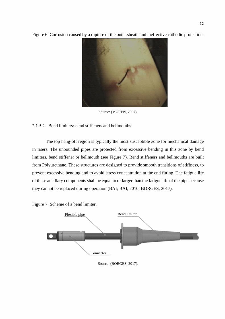
Bend limiters: bend stiffeners and bellmouths

The top hang-off region is typically the most susceptible zone for mechanical damage

in risers. The unbounded pipes are protected from excessive bending in this zone by bend

limiters, bend stiffener or bellmouth (see Figure 7). Bend stiffeners and bellmouths are built

from Polyurethane. These structures are designed to provide smooth transitions of stiffness, to

prevent excessive bending and to avoid stress concentration at the end fitting. The fatigue life

of these ancillary components shall be equal to or larger than the fatigue life of the pipe because

they cannot be replaced during operation (BAI; BAI, 2010; BORGES, 2017).

Figure 7: Scheme of a bend limiter.

Source: (BORGES, 2017).

Bend limiter Flexible pipe

Connector

13

Bend restrictors

Bend restrictors are structures, manufactured from metallic materials, creep-resistant

elastomers or fibre-glass-reinforced plastic (see Figure 8). They are designed to control the

bending of the flexible pipe, preventing overbending during installation or operation. “The

restrictor consists of interlocking half rings that fasten together around the pipe so that they do

not affect the pipe until a specified bend radius is reached, at which stage they lock”

(AMERICAN PETROLEUM INSTITUTE, 2008, p. 26). When the bend restrictors are in the

locked position, they support the additional loads, preventing further bending of the pipe.

Figure 8: Bend restrictor.


Subsea buoys and buoyancy modules

Subsea buoys are installed to achieve S-shaped riser configurations and to provide a

reduction on the top tension loads (see Figure 9). The structures are manufactured from steel or

synthetic foam. Buoyancy modules can be attached to the pipe in order to provide uplift and

maintain the specific riser configurations. The buoyancy elements are manufactured from

synthetic foam involved by polyurethane casing. The casing provides impact and abrasion

resistance, while the foam offers the uplift (AMERICAN PETROLEUM INSTITUTE, 2008;

TRELLEBORG, 2018).

Flexible pipe

Bend limiter

14

Figure 9: Subsea buoys connected to flexible pipes.

Source: (WORLEYPARSONS, 2015).

Risers configurations

Figure 10 illustrates examples of riser configurations recommended by the API RP 17B

standard. The geometric configuration of unbounded flexible pipes reflects the physical

demands on the structure, including self-weight and all other static and dynamic loads

respective to assembly and operation. The most critical sections are where the tensile forces are

higher, usually at the top, or at large curvatures, sag or hog bends. Therefore, each configuration

must be selected to reduce the mechanical stress while keeping the structure economically

viable. For example, free-hanging catenary minimises the costs by reducing the total length of

the pipeline and usage of ancillary components. However free-hanging catenary is not always

applicable given the large stresses found at the topside. Steep-S, Steep Wave, Lazy-S and Lazy

Wave configurations aim to reduce top traction due to the weight of the duct itself and minimise

the effect of platform movements in the region where the flexible duct rests on the seabed

(AMERICAN PETROLEUM INSTITUTE, 2008; BORGES, 2017).

Steep Wave and Lazy Wave configurations contain buoyancy and weight along the

length of the riser. The emphasis is on decoupling the vessel motions from the touch down point

of the riser. On the one side, Lazy Wave layout require minimal subsea infrastructure, on the

other side Steep Wave configuration require a subsea base and subsea bend stiffener. Steep

Wave configuration have the advantage of maintaining configuration when the fluid density

changes (BAI; BAI, 2019).

15

In the S-type configurations (Steep-S and Lazy S) a subsea buoy or a buoyant buoy are

employed to reduce the risk of mechanical damage in the touchdown point, because the buoy

absorbs the loads induced by the floater and the structure at the touchdown point. Due to the

complex installation, S-type configurations are only considered if catenary and wave

configurations are not suitable (BAI; BAI, 2019). “A lazy-S configuration requires a mid-water

arch, tether and tether base, while a steep-S requires a buoy and subsea bend stiffener (BAI;

BAI, 2019, pg. 403)”.

Figure 10: Five examples of riser configurations recommended by Standard API RP 17B.

Source: (AMERICAN PETROLEUM INSTITUTE, 2008).

High strength steels (HSS)

Pipes designed for deeper wells often employ high strength steels (HSS), because they

are cost-efficient solutions to support the mechanical loads generated by the associated high

pressures and the self-weight of the structure. However, there is relatively little information on

a) Free-hanging catenary

b) Steep-S c) Lazy-S

d) Steep wave e) Lazy wave

16

the corrosion resistance of these kinds of steels operating under such conditions in the open

literature.

2.2. GENERAL ASPECTS OF CORROSION

Corrosion can be defined as the natural process of materials returning towards lower

states of energy by the action of chemical and electrochemical reactions. The corrosion of

materials occurs on the surface after the contact of a product to an aggressive environment.

Corrosion should often be taken as a multidisciplinary process as several factors affect the

process, such as the nature of the reactions, the corrosion mechanisms, the metallurgy, the

geometry, the mechanical loads, the tides and the winds.

Nature of corrosion

The nature of corrosion is defined as the combination of all relevant interactions

between the environment and the materials. Accurate characterisations can be quite complex as

the environment, and the surface of the material may change with time or due to an uncountable

number of variables. Nonetheless, dedicating effort to identify the nature of corrosion is always

advisable for corrosion assessments, since numerous steps would follow.

Aqueous corrosion

Aqueous corrosion is the degradation of materials in aqueous environments. It is quite

common in nature and engineering problems, particularly to those related to the offshore oil

and gas industry as a large number of structures and equipment remain underwater for long

periods. Aqueous corrosion is essentially electrochemical, always involving two or more redox

reactions taking place on the metal surface. The process requires the formation of a corrosion

cell, which is described by four essential parts: the anode, the cathode, the electronic path and

the ionic path (see Figure 11).

17

Figure 11: General requirements for a corrosion process.

Source: Adapted from (DAVIS, 2000).

The corrosion begins when an oxidation reaction initiates at the anode, resulting in the

loss of electrons and release of ions in the solution (Mn+), see the generalised reaction in

equation 1. The electrons lost by the anode, move towards the cathode by an existing electronic

path, establishing a direct current between parts. The movement of electrons is essential for the

existence and continuity of the reduction reactions because the electrons lost by the anode are

the ones involved in the reduction reactions at the cathode. The ionic path is also indispensable

for the continuity of the process. In particular, because the dissolved ions must be somehow be

transported between the anode and the cathode. Otherwise, in the absence of ions to be reduced,

the degradation of the material would stop. Notice, for instance, that coating metals with paints

or protective scales are effective methods to prevent corrosion because they suppress the

movement of ions. Hence, it shall be stressed that all electrochemical constitutive parts must

exist for the existence of an aqueous corrosion process. The suppression of one or more

elements terminates the corrosion immediately (DAVIS, 2000; GENTIL, 2011).

M → Mn+ + ne (1)

Atmospheric corrosion

Atmospheric corrosion can be defined as the chemical or electrochemical deterioration

when the material remains in contact to the atmospheric air. It begins in the presence of

humidity or condensed water or high temperatures. Climate factors and pollutants are also

known causes capable of changing the aggressiveness of the environment (ROBERGE, 2000;

SYED, 2010).

Atmospheric corrosion is classified according to the level of humidity, which is dry

atmospheric corrosion, humid atmospheric corrosion or wet atmospheric corrosion. The first

typically involves chemical mechanisms, characterised by slow degradation of metals in dry

Electronic path

Anode Cathode

Ionic current path

𝑀 → 𝑀𝑛+ + 𝑛𝑒 𝑛𝐻+ + 𝑛𝑒 → 𝑛/2𝐻2

18

atmospheres, the tarnishing of silver is a typical example. The second consists of the corrosion

of metals in environments presenting relative humidity below 100%, where a thin layer of

electrolyte remains in contact with the surface of the metal. In this case, the corrosion rates

change according to the relative humidity and the presence of noxious species. Finally, the third

type involves environments presenting condensed water in contact with the metallic surface,

where the relative humidity is very close to 100%. It has been reported that the structural layers

confined in the annulus of unbounded flexible pipes may experience the condensation of water;

thus, atmospheric corrosion may occur in the structural layers of flexibles (ERIKSEN;

ENGELBRETH, 2014; GENTIL, 2011; UNDERWOOD, 2002).

Galvanic corrosion

Galvanic corrosion is experienced after the electrical contact between two or more

dissimilar metals submerged in the same solution. Accordingly, the more active metal suffers

an intense attack, while the more noble metal is usually protected or has its corrosion rate greatly

decreased. The galvanic coupling may induce changes in the morphology, including the growth

of protective scales and build-up of passive layers. The driving force is the electrochemical

potential difference between metals, forcing the electrons to flow (AMERICAN SOCIETY

FOR TESTING AND MATERIALS, 2012, 2014a, 2014b; BABOIAN et al., 1976).

In general, galvanic corrosion is studied by the Mixed Potential Theory (MPT). MPT is

based on the assumption that the electrochemical reactions are divided into two or more

reactions (oxidation and reduction), and that there can be no net accumulation of electrical

charge during the process. A general rule-of-thumb to prevent the risk of galvanic corrosion is

avoiding large electrochemical potential differences between the anode and cathode. Thus,

materials are often ranked into galvanic series that work as guidelines for material selections.

Materials which remain close in the galvanic series shall not suffer from strong galvanic

corrosion. Despite that, the galvanic series describe specific combinations of materials and

environments, meaning that any variations of the electrochemical potential might affect the

galvanic behaviour, for example changing the morphology of the surface or the electrolyte

(AMERICAN SOCIETY FOR TESTING AND MATERIALS, 2012, 2014a, 2014b;

BABOIAN et al., 1976).

19

Thermodynamics of corrosion

The concepts of thermodynamics are settled on a fundamental law of nature, in which

the state of a material is always driven towards equilibrium, where the lowest state of free

energy is found. Thermodynamics defines the influence of environmental aspects on the

degradation of materials in equilibrium; it describes the moment when there is no measurable

exchange of energy between a reactant and a product. Notice that this does not mean that the

reactions would stop, rather than the rate of the reaction moving forward (Rf) would equal the

rate moving backwards (Rb). Assuming the system described in equation 2, the equilibrium is

mathematically characterised by the equilibrium constant, which is a function of the activities

of the chemical species, equation 3. The terms “W” and “X” are the reactants; “Y” and “Z” are

the products; “w”, “x”, “y”, “z” are the stoichiometric coefficient of the main components;

“aW”, “aX”, “aY”, “aZ” are the activities of the main species. The concepts of activities are used

to describe the effective concentration of species in a mixture. In other words, whenever there

is a difference between ideal and observed properties of a solution (DAVIS, 2000).

wW+ xX ↔ yY + zZ (2)

Ka = (aYyaZz

aWw aX

x) , when Rf = Rb (3)

Furthermore, thermodynamics is used to predict if a corrosive process can occur

spontaneously or not. This information is revealed through the concepts of Gibbs free-energy

(G). The term“G” defines the highest amount of mechanical energy that can be obtained by a

substance without changing its state properties, meaning that G should be a function of state

variables such as pressure (P), temperature (T) and the number of moles of given substance in

a mixture (nn), see equation 4. According to Gibbs (1873, p400), “[…] the equilibrium of the

body is unstable regarding discontinuous changes, a certain amount of energy will be available

under the conditions for the production of work […]”.

G → f(P, T, nn) (4)

As well as it occurs with electrical potentials, the primary importance of G does not lie

on the absolute values, rather than in the variations, as ∆G reflects the chemical energy available

for doing mechanical work. ∆G is mathematically determined by equation 5. The signal of ∆G

20

carries the information regarding the spontaneity of the reaction. If ∆G is negative, then the

reaction can occur spontaneously. When ∆G is equal to zero, there is no energy available to

change the state of the substance, which means that the reaction remains in equilibrium.

However, if ∆G is positive, then it is possible to change the state of the substance non-

spontaneously, meaning that energy should be added to the system. Figure 12 shows the free-

energy diagrams for each situation. The dependence of G on the state properties, such as

temperature, could explain why some materials oxidise at elevated temperatures but not at

ambient conditions. In other words, this means that sources of energy like heat can enhance the

chemical energy available for reactions to occur on the surface of materials (AMERICAN

SOCIETY FOR METALS INTERNATIONAL, 2003; DAVIS, 2000; GENTIL, 2011).

∆G = ∆G0 + RT. ln(Ka) (5)

Figure 12: Free-energy diagrams.


∆G is often converted into electrical potentials to rank the oxidation or reduction

tendencies of several materials in series. The conversion is achieved employing equations 6 to

8. The term “Ԑ” is the difference in the electric potential, “Ԑ0” is the electric potential under the

standard states, “F” is the Faraday constant (96,487 coulomb/mol), “n” is the number of

electrons exchanged and “øi” is the potential to move an electrical charge between two points.

Such conversion is convenient to predict which direction the corrosion process could occur,

once the noblest materials remain protected at the expense of the deterioration of the most active

materials. Figure 13 shows an electrode potential ranking for seawater at 25 °C. The noblest

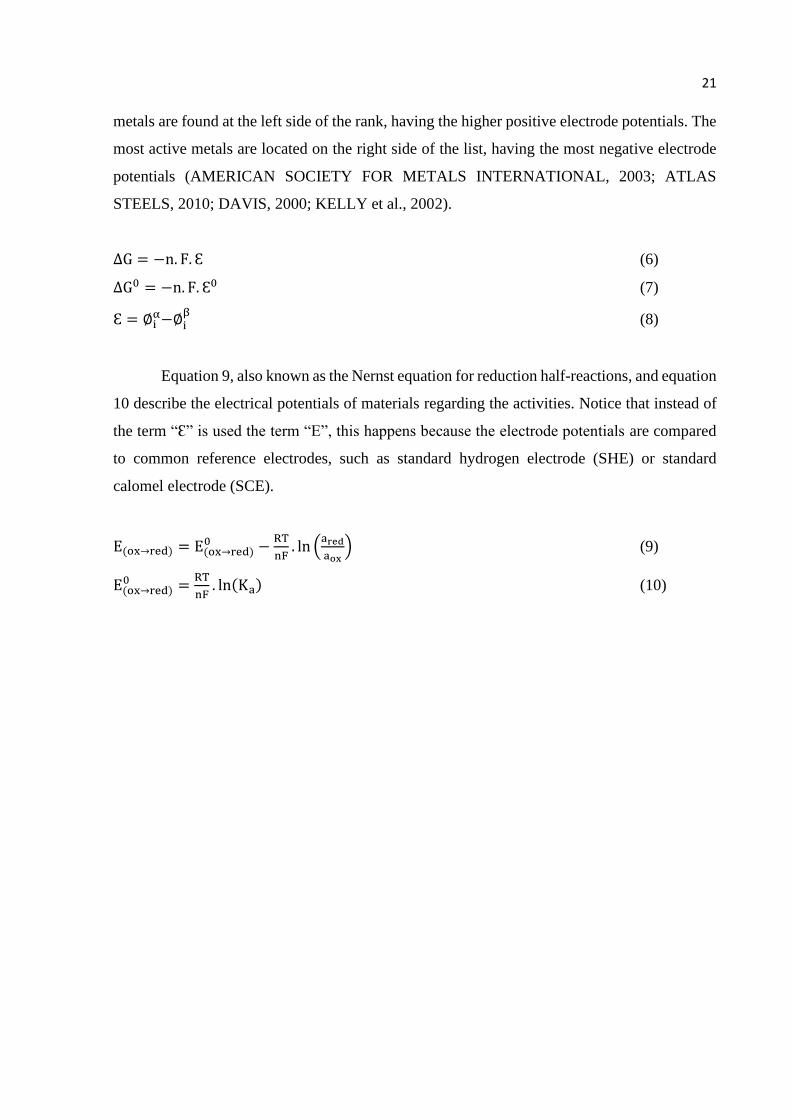
21

metals are found at the left side of the rank, having the higher positive electrode potentials. The

most active metals are located on the right side of the list, having the most negative electrode

potentials (AMERICAN SOCIETY FOR METALS INTERNATIONAL, 2003; ATLAS

STEELS, 2010; DAVIS, 2000; KELLY et al., 2002).

∆G = −n. F. Ԑ (6)

∆G0 = −n. F. Ԑ0 (7)

Ԑ = ∅iα−∅i

β (8)

Equation 9, also known as the Nernst equation for reduction half-reactions, and equation

10 describe the electrical potentials of materials regarding the activities. Notice that instead of

the term “Ԑ” is used the term “E”, this happens because the electrode potentials are compared

to common reference electrodes, such as standard hydrogen electrode (SHE) or standard

calomel electrode (SCE).

E(ox→red) = E(ox→red)0 −

RT

nF. ln (

ared

aox) (9)

E(ox→red)0 =

RT

nF. ln(Ka) (10)

22

Figure 13: Electrode reduction potentials of metals (VSCE), for seawater at 25 °C. The unshaded

symbols show ranges exhibited by stainless steels in acidic water, which could be

related to occlusion and aeration aspects.

Source: (ATLAS STEELS, 2010).

Pourbaix diagrams

Based on the notions of chemical potential and affinity, it is possible to predict the

circumstances in which electrochemical reactions are energetically possible or impossible. In

other words, the equilibrium characteristics of electrochemical reactions at given environments

can be represented by a point on a diagram of pH and potential (E), which derives from the

Nernst equation (equation 9). The projection of the point in the diagram reveals the likely

thermodynamic outcome of the contact between the material and the given environment.

(AMERICAN SOCIETY FOR METALS INTERNATIONAL, 2003; AZOULAY, 2013;

GHALI, 2010; POURBAIX, 1945, 1987; ROBERGE, 2000; TANUPABRUNGSUN et al.,

2012; UNIVERSITY OF CAMBRIDGE, 2018).

23

E-pH diagrams are powerful tools for corrosion control, materials selection and for

understanding the formation of scales formed by the action of nature or due to accelerated

corrosion tests. Figure 14 shows an example of the equilibrium diagram of pure iron in water,

taken from the original thesis of Marcel Pourbaix (POURBAIX, 1945).

Figure 14: Fe-H2O Pourbaix diagram.

Source: Adapted from (POURBAIX, 1945).

The borderlines of the diagram represent the frontiers of stability for the electrochemical

reactions. Three domains are revealed: (i) dissolution, (ii) passivity and (iii) immunity. Each

domain can be associated with a particular condition of stability and corrosion surface (see

Figure 15). The dissolution is related to active surfaces experiencing weight loss. Passivity is

associated with surfaces containing insoluble and adherent protective corrosion products,

experiencing very mild corrosion rates. Immunity is associated with the surfaces presenting

thermodynamic stability on the given environment, when corrosion is unable to occur

spontaneously.

(iii) Immunity

(i) Dissolution

(ii) Passivity

pH

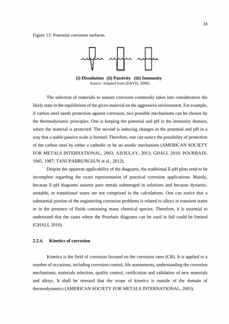
24

Figure 15: Potential corrosion surfaces.


The selection of materials to sustain corrosion commonly takes into consideration the

likely state in the equilibrium of the given material on the aggressive environment. For example,

if carbon steel needs protection against corrosion, two possible mechanisms can be chosen by

the thermodynamic principles. One is keeping the potential and pH in the immunity domain,

where the material is protected. The second is inducing changes in the potential and pH in a

way that a stable passive scale is formed. Therefore, one can notice the possibility of protection

of the carbon steel by either a cathodic or by an anodic mechanism (AMERICAN SOCIETY

FOR METALS INTERNATIONAL, 2003; AZOULAY, 2013; GHALI, 2010; POURBAIX,

1945, 1987; TANUPABRUNGSUN et al., 2012).

Despite the apparent applicability of the diagrams, the traditional E-pH plots tend to be

incomplete regarding the exact representation of practical corrosion applications. Mainly,

because E-pH diagrams assume pure metals submerged in solutions and because dynamic,

unstable, or transitional states are not comprised in the calculations. One can notice that a

substantial portion of the engineering corrosion problems is related to alloys in transient states

or in the presence of fluids containing many chemical species. Therefore, it is essential to

understand that the cases where the Pourbaix diagrams can be used in full could be limited

(GHALI, 2010).

Kinetics of corrosion

Kinetics is the field of corrosion focused on the corrosion rates (CR). It is applied to a

number of occasions, including corrosion control, life assessments, understanding the corrosion

mechanisms, materials selection, quality control, verification and validation of new materials

and alloys. It shall be stressed that the scope of kinetics is outside of the domain of

thermodynamics (AMERICAN SOCIETY FOR METALS INTERNATIONAL, 2003).

(i) Dissolution (ii) Passivity (iii) Immunity

25

The rate at which a material deteriorates in a given environment can be expressed by

many units, such as the penetration rate, the rate of weight loss or the current density. Various

methods can be used to measure corrosion rates, including weighing coupons with known

weight after submersion in aggressive fluids, for determining the average corrosion rates. Other,

and more complex electrochemical techniques, such as linear sweep voltammetry (LSV), cyclic

voltammetry (CV) and linear polarisation resistance (LPR) may also be employed with the

advantage of describing corrosion properties, such as: corrosion potentials, polarisation

resistance, resistance of the electrolyte and Tafel slopes (AMERICAN SOCIETY FOR

TESTING AND MATERIALS, 1989, 1997, 2003, 2014c; RIBEIRO, 2014).

Electrochemical methods are commonly preferred for laboratory testing because of the

high degree of specificity offered in relatively short periods. These techniques usually describe

the corrosion rates by sweeping or disturbing the electric potential (or current) of the material

of interest, also known as the working electrode (WE). The underlying assumption behind

electrochemical testing is that the corrosion rate of a material is proportional to the electric

current passing through the components of the system. The combination of the generalised

oxidation reaction (equation 1), equation 6 and the Arrhenius expression (equation 11) results

in equation 12, which reveals the exponential relationship between electric current with the

overpotential (η). The term “k” is the rate of the reaction and “C” is a constant. The term “ηa”

defines the difference between artificially driven potential (anodic) and equilibrium potential.

“Ia” is the term used for anodic current, “I0” for the current flowing in both directions when an

electrode reaction is at equilibrium and “α” is a symmetry factor. The step-by-step description

to obtain equation 12 can be found in the literature (AMERICAN SOCIETY FOR METALS

INTERNATIONAL, 2003; UNIVERSITY OF CAMBRIDGE, 2018).

M → Mn+ + ne (1)

∆G = −n. F. Ԑ (6)

k = C e[−∆G

RT⁄ ] (11)

Ia = I0 e[αnFηa

RT⁄ ] (12)

Equation 12 is also known as one form of the Tafel equation, which can be adjusted to

obtain equation 13. Accordingly, “ba” is the Tafel slope, and “Ca” a constant. Moreover, because

the reactions are essentially electrochemical rather than chemical, the anodic and cathodic

currents can be studied independently and should share equal magnitudes. Therefore, a similar

26

approach can be followed for the cathodic reactions, which results in equation 14. In this case,

“bc” is the cathodic Tafel slope and “Cc” a cathodic constant.

𝜂𝑎 = 𝐶𝑎 + 𝑏𝑎 log10 𝑖𝑎 (13)

𝜂𝑐 = 𝐶𝑐 + 𝑏𝑐 log10 𝑖𝑐 (14)

The Tafel slopes are defined as measures of energy barrier symmetry of the potential

energy curves. They can be calculated by equation 15 when all of the reactions involved in the

corrosion process are known in depth. Otherwise, the Tafel slopes are estimated from the slopes

at the linear portions of semi-log plots i x E, as shown in Figure 16 (AMERICAN SOCIETY

FOR TESTING AND MATERIALS, 1989, 1997, 2014c; ROBERGE, 2000).

𝑏𝑎,𝑐 =2.303. 𝑅𝑇

𝛼𝑛𝐹⁄ (15)

Figure 16: Hypothetical scheme of a polarisation diagram.

Source: (AMERICAN SOCIETY FOR TESTING AND MATERIALS, 2014c).

27

Electrochemical corrosion mechanisms

The corrosion phenomena of metals involve a great variety of mechanisms that are

grouped according to the nature of the corrosion. This work focusses on the electrochemical

degradation of metals in aqueous environments. Under such circumstances, the corrosion of

metals often occurs by charge-transfer or diffusion controlled or even mixed-mechanisms. Each

one presents its specific behaviour regarding the corrosion rates. For example, the charge-

transfer mechanism, also known as activation-control, can be identified by the linear behaviours

on semi-log plots of current density (i) versus potential (E). The second mechanism, called

diffusion controlled, refers to the corrosion process where the concentration of a particular

chemical cannot be sustained at the same level as that in the bulk of the solution, so the process

becomes controlled exclusively by the transport of chemical species from the bulk solution to

the metal-electrolyte interface. This way, any factor changing the diffusive or advective

properties, such as fluid velocity, shall disturb the corrosion rates. These mechanisms are

visualised in Figure 17, where linear voltammetry sweeps were performed in rotating

electrodes. The overlapping straight lines, seen in the anodic branches, reveal the charge-

controlled mechanism, once the diffusive and advective factors show no impact on the current

density. The portion of the plot with non-overlapping corrosion densities, seen in the cathodic

branches, reveals the mass-controlled mechanism, where the relative velocities between the

working electrodes and electrolyte change the supply of reactants available for the redox

reactions, thus impacting on the current density (HERNANDEZ; MUÑOZ; GENESCA, 2012).

Figure 17: Polarisation curves of steel at different rotation rates. A test carried in brine solution

saturated with carbon dioxide at 20 °C.

Source: Adapted from (HERNANDEZ; MUÑOZ; GENESCA, 2012).

0 RPM

5000 RPM

10 10 10

///

10

///

10

///

10

///

10

///

28

2.3. ANNULUS ENVIRONMENT

The annulus was initially designed to operate under dry conditions. However, reality

shows that it evolves into very complex environment, whose severity hinge on numerous

factors, such as the atmospheric variables, the composition of the solution, the operating

conditions, the geometric factors and the integrity of the outer sheath. And, many of these vary

along the pipe length and depth.

The large gradients of pressure and temperature in which the wires are located widen

the complexity of the discussion, given their effects on kinetics and chemistry of the

environment and materials. According to modern knowledge, the temperatures in the annulus

should range between 20 and 80 °C, where the variations are a function of the temperature

difference between the fluid running in the bore and the seawater surrounding the pipe. Pressure

is essentially depth dependent; thus, segments of the pipelines operating at deeper wells may

experience more severe hydrostatic pressures. Hence, the following chapters shed light on

crucial issues regarding the flooding and permeation of fluids towards the annulus, the

interactions between liquid and gaseous phase interactions, and the specific hydrochemistry of

carbon dioxide (CHEMISTRY BLOG, 2018; CLEMENTS, 2008; CLEMENTS; ETHRIDGE,

2003; DÉSAMAIS; TARAVEL-CONDAT, 2009; DUGSTAD et al., 2015; FERGESTAD;

LØTVEIT, 2014; KE et al., 2017; NEŠIĆ, 2007; NOV, 2015; ROGOWSKA et al., 2016;

ROPITAL et al., 2000; RUBIN et al., 2012; UNDERWOOD, 2002).

Breaches of the outer polymer sheath

The outer polymer sheath is a constitutive layer of the unbounded flexible pipe designed

to prevent direct contact between seawater and the structural wires. The failure of this layer is

one of the leading threats to unbounded flexible pipes, because it enables conditions for

considerable corrosion on the structural layers of the pipe. Breaches can be associated with

many causative factors, including blockage of the venting system, impact damage, abrasion,

non-conformities during installation and operation. According to 4SUBSEA (2013), avoiding

damages to the outer sheath could mitigate the corrosion process of the structural layers of the

pipe. However, it seems very unlikely that industry will manage to eradicate them in the short-

term. Keeping that in mind, the understanding of the corrosion mechanisms and variables

affecting the environment are essential to improve prediction and capabilities of the technology

29

(4SUBSEA, 2013; ERIKSEN; ENGELBRETH, 2014; FERGESTAD; LØTVEIT, 2014; JOEL,

2009).

Permeation of fluids into the annulus

Although the internal and outer polymer sheaths of the annulus are designed to prevent

the direct contact to the internal fluid and surrounding seawater, modern flexible pipes remain

susceptible to ingress of water and gases through permeation processes into the annulus. The

polymer layers exhibit a certain level of permeability towards water, carbon dioxide, methane

and hydrogen sulphide (see Figure 18). The fluid permeation can be unidirectional or

bidirectional, i.e. between the bore and the annulus or between the annulus and the seawater in

the surroundings (BORGES, 2017).

Figure 18: Schematic illustration of the permeation of gases from the bore into the annulus

region.

Source: AUTHOR.

The understanding of the transport mechanisms of the fluids into the annulus and the

consequent damage to the structural layers of the pipe is still very far from satisfactory, as

thermodynamic and kinetic aspects are yet poorly understood. For example, the permeation rate

is usually interpreted as a kinetic variable; however, studies exploring the effect of low flow

rates on the risk of sulphide stress corrosion cracking in H2S-containing environments identified

that the restricted permeation rates could influence the steady state concentration of this

aggressive species in the simulated annulus conditions. These studies point out that the

permeation rates tend to be low compared to consumption by the corrosion of the large surface

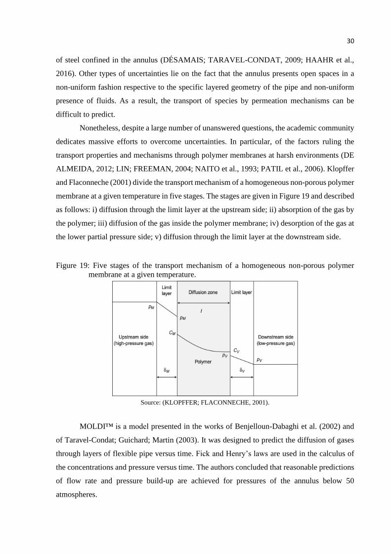
30

of steel confined in the annulus (DÉSAMAIS; TARAVEL-CONDAT, 2009; HAAHR et al.,

2016). Other types of uncertainties lie on the fact that the annulus presents open spaces in a

non-uniform fashion respective to the specific layered geometry of the pipe and non-uniform

presence of fluids. As a result, the transport of species by permeation mechanisms can be

difficult to predict.

Nonetheless, despite a large number of unanswered questions, the academic community

dedicates massive efforts to overcome uncertainties. In particular, of the factors ruling the

transport properties and mechanisms through polymer membranes at harsh environments (DE

ALMEIDA, 2012; LIN; FREEMAN, 2004; NAITO et al., 1993; PATIL et al., 2006). Klopffer

and Flaconneche (2001) divide the transport mechanism of a homogeneous non-porous polymer

membrane at a given temperature in five stages. The stages are given in Figure 19 and described

as follows: i) diffusion through the limit layer at the upstream side; ii) absorption of the gas by

the polymer; iii) diffusion of the gas inside the polymer membrane; iv) desorption of the gas at

the lower partial pressure side; v) diffusion through the limit layer at the downstream side.

Figure 19: Five stages of the transport mechanism of a homogeneous non-porous polymer

membrane at a given temperature.

Source: (KLOPFFER; FLACONNECHE, 2001).

MOLDI™ is a model presented in the works of Benjelloun-Dabaghi et al. (2002) and

of Taravel-Condat; Guichard; Martin (2003). It was designed to predict the diffusion of gases

through layers of flexible pipe versus time. Fick and Henry’s laws are used in the calculus of

the concentrations and pressure versus time. The authors concluded that reasonable predictions

of flow rate and pressure build-up are achieved for pressures of the annulus below 50

atmospheres.

31

Henry’s law of solubility

The earliest studies on the solubility of carbon dioxide in water date from the beginning

of the 19 century, where the work of William Henry (1803) constitutes the building block for

the law of solubility, also known as Henry’s law of solubility (equation 16). According to Henry

(1803), the amount of dissolved gas is proportional to its partial pressure of a chemical specie

(pP) and to an equilibrium constant (KH), which is named as Henry’s constant. More precisely,

the effect of pressure on the solubility is given along these lines:

[…] that, under equal circumstances of temperature, water takes up, in all cases, the

same volume of condensed gas as of gas under ordinary pressure. But, as the spaces

occupied by every gas are inversely as the compressing force, it follows, that water

takes up, of gas additional atmospheres, a quantity which, ordinarily compressed,

would be equal to twice, thrice, etc. the volume absorbed under the common pressure

of the atmosphere.[…] (HENRY, 1803, p.41).

Solubility = KH′ . pP (16)

Henry (1803) also observed that the quantity of carbon dioxide dissolved in the solution

tends to decrease with the increase of temperature. Such tendency is related to the effect of

temperature on the equilibrium constant KH. Methods to obtain accurate values of KH are

outside the scope of this work but can be obtained in the literature as a function of temperature

(van ’t Hoff equation) or the Gibbs free-energy (MAJER; SEDLBAUER; BERGIN, 2008;

SANDER, 2015).

Though modern knowledge agrees with Henry’s law of solubility at low to moderate

pressures, the relationship proposed by Henry is constrained by simplifications. For example,

Henry's constant neglects the effect of pressure and assume that activity equals the

concentration. Therefore, although Henry’s law was developed to describe the effect of

temperature and gas pressure on the solubility of the gaseous species in water, his work is

restricted to circumstances where liquid phase non-idealities can be neglected. Outside this

domain, modern studies usually focus on the description of systems by means of modelling and

correlations from empirical data.

Figure 20 and Figure 21 show, respectively, the effects of temperature and pressure in

the solubility of CO2 in water (AQION, 2018; CARROLL; SLUPSKY; MATHER, 1991;

HANGX, 2005; OLI STUDIO, 2016).

32

Figure 20: Effect of temperature on the solubility of carbon dioxide in water.

Source: (HANGX, 2005).

Figure 21: Effect of pressure on the solubility of carbon dioxide in water.

Source: (HANGX, 2005).

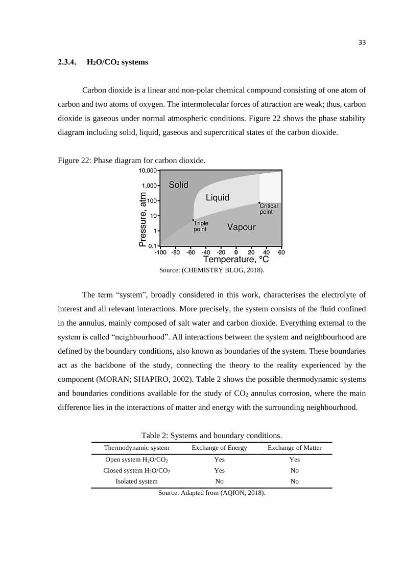
33

H2O/CO2 systems

Carbon dioxide is a linear and non-polar chemical compound consisting of one atom of

carbon and two atoms of oxygen. The intermolecular forces of attraction are weak; thus, carbon

dioxide is gaseous under normal atmospheric conditions. Figure 22 shows the phase stability

diagram including solid, liquid, gaseous and supercritical states of the carbon dioxide.

Figure 22: Phase diagram for carbon dioxide.

Source: (CHEMISTRY BLOG, 2018).

The term “system”, broadly considered in this work, characterises the electrolyte of

interest and all relevant interactions. More precisely, the system consists of the fluid confined

in the annulus, mainly composed of salt water and carbon dioxide. Everything external to the

system is called “neighbourhood”. All interactions between the system and neighbourhood are

defined by the boundary conditions, also known as boundaries of the system. These boundaries

act as the backbone of the study, connecting the theory to the reality experienced by the

component (MORAN; SHAPIRO, 2002). Table 2 shows the possible thermodynamic systems

and boundaries conditions available for the study of CO2 annulus corrosion, where the main

difference lies in the interactions of matter and energy with the surrounding neighbourhood.

Table 2: Systems and boundary conditions.

Thermodynamic system Exchange of Energy Exchange of Matter

Open system H2O/CO2 Yes Yes

Closed system H2O/CO2 Yes No

Isolated system No No

Source: Adapted from (AQION, 2018).

34

The open system H2O/CO2 allows the exchange of energy and matter, meaning that the

natural processes of materials returning towards lower states of energy are free to exist. Also,

this system is not bound by finite amounts of matter, so the sum of all chemical species may

not be constant. On the other hand, closed system H2O/CO2 is characterised by containing finite

and well-defined amounts of matter in the system, as the exchange of mass with the

neighbourhood is forbidden. In practice, this means that the growth of the concentration of one

species is limited to the total concentration of anothers because the mass balance must remain

constant. Isolated systems are not explored here because they seem unrealistic for the purpose

of this work, given their complete isolation from the neighbourhood regarding energy and

matter.

Hydrochemistry

Hydrochemistry is the branch of science that studies the chemical composition of natural

waters and the laws governing its changes. Understanding the particular hydrochemistry of

water/carbon dioxide systems is essential to obtain indications of the aggressiveness and

permeation properties of the environment, since CO2-corrosion is a synergic process involving

chemical, electrochemical and mass transport reactions (BARKER et al., 2018; CARROLL;

SLUPSKY; MATHER, 1991; DE ALMEIDA, 2012; DÉSAMAIS; TARAVEL-CONDAT,

2009; HAAHR et al., 2016; NEŠIĆ, 2007; SANTOS et al., 2013; TARAVEL-CONDAT;

GUICHARD; MARTIN, 2003).

In open systems composed of water and carbon dioxide, the interactions begin with the

hydration of carbon dioxide (equation 17), followed by the formation of carbonic acid (equation

18). At this point, the carbonic acid dissociates twice (equation 19 and equation 20), releasing

hydrogen (H+), bicarbonate (HCO3-) and carbonate (CO3

-2) in the water. The self-ionization of

water (equation 21) also takes place in the full description of the chemical reactions.

CO2(g)⇔CO2(aq) (17)

CO2(aq) + H2OKH⇔H2CO3 (18)

H2CO3(aq)K1⇔H+ + HCO3

− (19)

HCO3−K2⇔H+ + CO3

2− (20)

H2OKw⇔ H+ + OH− (21)

35

The full characterisation of open H2O/CO2-systems requires the quantification of 6

chemical species (CO2(aq), H2CO3, HCO3-, CO3

-2, H+ and OH-) and four equilibrium constants

(KH, K1, K2, Kw), totalling ten variables. However, all equilibrium constants can be obtained

from specific pressure-temperature tables available in the literature (MAJER; SEDLBAUER;

BERGIN, 2008; SANDER, 2015). With this simplification, the required number of equations

would drop to six. The remaining equations needed, can be obtained by employing the mass-

action law and performing mass and charge balances. In which, assuming ideally diluted

solutions the system is specified from equation 22 to 27. Note that the carbonate ion in equation

27 is multiplied by a factor of 2 because of the divalent charge (AQION, 2018; MOHAMED et

al., 2011; OLI STUDIO, 2016).

Mass-action law: KH = [H2CO3]/pCO2 (22)

Mass-action law: K1 = [H+][HCO3

−]/[H2CO3] (23)

Mass-action law: K2 = [H+][CO3

−2]/[HCO3−] (24)

Mass-action law: Kw = [H+][OH−] (25)

Mass balance: DIC = [H2CO3] + [HCO3−] + [CO3

2−] (26)

Charge balance: [H+] = [HCO3−] + 2[CO3

2−] + [OH−] (27)

The same set of equations is also used for the characterisation of closed H2O/CO2-

systems. However, closed systems present the additional limitation of finite amounts of matter,

which is represented by the constant value of dissolved inorganic carbon (DIC). As a result, the

formation of carbonic acid is not only a function of equation 22 but also restricted by the total

DIC available in the system. Although the differences between open and closed carbonate

systems are well understood, this subject is poorly addressed in the literature. Hence, such

differences are contained within the scope of this work, meaning that further details are

provided in the section of results and discussion.

2.4. CORROSION OF UNBOUNDED FLEXIBLE PIPES

Figure 23 shows a list of some variables that may affect the corrosion of unbounded

flexible pipes. It is assumed that the process is complex and multidisciplinary, involving the

hydrochemistry of seawater, operating conditions, aspects of design and assembly of the pipes

36

and corrosion mechanisms. Also, despite the focus on occluded CO2-corrosion of flexible pipes

dedicated to this work, the literature review also includes the effect of depth and bulk corrosion

given the possibility of the structural layers of the pipe remain directly in contact to seawater

as a result of unrepaired damages in the outer layer of the flexibles.

Figure 23: Examples of variables that can affect the corrosion process of unbounded flexible

pipes.

Source: AUTHOR.

Effect of depth on the corrosion of subsea structures

Though the water surrounding the pipe should not be in direct contact to the structural

layers of the flexible pipes under normal conditions, ruptures and failures of the outer sheath

are common, exposing the structural layers of the pipe to corrosion. It is known that many

variables are a function of depth, including the hydrostatic pressure, the temperature and the

chemical composition of seawater. Recognising this information is essential to understand the

effects of depth on the corrosion of subsea structures.

A study of a steel piling submersed in seawater, described in Davis (2000), is used as

basis to demonstrate the effect of depth. It is reasonable to assume that unrepaired damages to

the structural layers of unbounded flexible pipes may undergo comparable trends of corrosion

37

rates. Accordingly, Figure 24 shows a sketch of the corrosion rates obtained from the steel

piling, where a total of five zones are revealed.

Figure 24: Corrosion rate of a steel piling in seawater.


The discussion begins at the deepest portion of the structure, zone 1, where the steel lies

submerged in the ocean mud. The mud often contains large quantities of organic material in

decomposition that produces a reductive atmosphere, containing low concentrations of oxygen.

This scenario implies in a reduction on the corrosion rates by constraining the cathodic reactions

(DAVIS, 2000). Equation 28 and equation 29 show typical examples of cathodic reactions for

aerated and de-aerated water respectively (GENTIL, 2011).

Aerated water: H2O(l) + 1/2O2(g) + 2e → 2OH(aq)− (28)

De-aerated water: H+ + e− ↔ 1 2⁄ H2(g) (29)

Zone two describes the portion where the metal is continuously submerged in the saline

aqueous environment. Throughout this section, the salinity of the water can be considered

approximately constant, around 35,000 ppm. However, as observed in Figure 25, the amount

of dissolved oxygen decreases with depth. Consequently, the corrosion rates also decrease with

depth due to the reduction of the concentration of oxygen (DAVIS, 2000; SCRIPPS

INSTITUTION OF OCEANOGRAPHY, 2013). Figure 26 shows the effect of a rupture of the

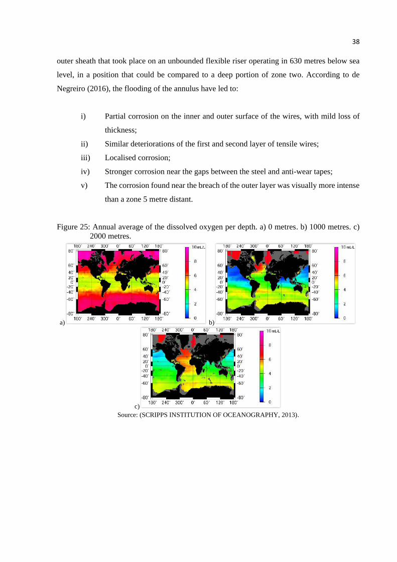
38

outer sheath that took place on an unbounded flexible riser operating in 630 metres below sea

level, in a position that could be compared to a deep portion of zone two. According to de

Negreiro (2016), the flooding of the annulus have led to:

i) Partial corrosion on the inner and outer surface of the wires, with mild loss of

thickness;

ii) Similar deteriorations of the first and second layer of tensile wires;

iii) Localised corrosion;

iv) Stronger corrosion near the gaps between the steel and anti-wear tapes;

v) The corrosion found near the breach of the outer layer was visually more intense

than a zone 5 metre distant.

Figure 25: Annual average of the dissolved oxygen per depth. a) 0 metres. b) 1000 metres. c)

2000 metres.

Source: (SCRIPPS INSTITUTION OF OCEANOGRAPHY, 2013).

a) b)

c)

39

Figure 26: Images of the inner tensile layer of an unbonded flexible pipe. a) Shows the corroded

wires without the presence of the anti-wear tape and b) shows the anti-wear tape.

Source: (DE NEGREIROS, 2016).

Zone three refers to the portion affected by the tides zone. This zone is favourable to the

biological species that may protect the steel against the seawater, so the corrosion rates tend to

reduce. As the depth decrease, a section of the pilling remains alternately submerged in

seawater. Consequently, corrosion rates tend to increase again because of the availability of

oxygen (DAVIS, 2000).

Zone four refers to the splash zone. This section presented the higher corrosion rates

found in the steel pilling because of the increased local salinity and high availability of oxygen.

The splashing of water leaves droplets, rich in chloride, on the surface of the steel. After

evaporation, the local salinity of the surface can increase considerably (DAVIS, 2000).

Zone five describes the portion of the pilling damaged by the atmospheric corrosion.

Since aqueous corrosion is generally more aggressive than atmospheric corrosion, the corrosion

rates tend to decrease gradually as the incidence of droplets in the structure decrease (DAVIS,

2000).

Bulk CO2-corrosion

Bulk CO2-corrosion is defined as the corrosive process occurring in environments rich

in carbon dioxide, in the presence of considerable volumes of water. A peculiarity of CO2-

corrosion is that a substantial number of parameters may significantly influence it, and the

interactions between variables can be reasonably complex. Therefore, despite a large number

of works available in the literature, the phenomenon is still poorly understood. Hence, the

following chapters provide brief introductions to some subjects deemed pertinent to this work

(CROLET; THEVENOT; NEŠIĆ, 1998; DUGSTAD et al., 2015, 2018; FANG; BROWN;

NEŠIĆ, 2013; HAN et al., 2007; LIU et al., 2016; LOPEZ et al., 2003; LÓPEZ; PÉREZ;

Corrosion surface within the gaps between anti-wear tapes

40

SIMISON, 2003; NEŠIĆ, 2007; SCHMITT; HÖRSTEMEIER, 2006; SUHOR et al., 2012;

SUN, 2006; SUN; NEŠIĆ, 2008; TANUPABRUNGSUN et al., 2012; ZENG; LILLARD;

CONG, 2016).

Mechanisms of CO2-corrosion

Two possible charge-transfer mechanisms can be linked to the cathodic reactions. One

is the direct reduction mechanism that is attributed to the reduction of the adsorbed carbonic

acid molecule occurring at the metal surface, described from equation 29 to 32. The other

potential mechanism is the so-called “buffering effect”, in what the dominant cathodic reaction

is the reduction of hydrogen ions, whereas the dissociation of the carbonic acid provides

additional hydrogen ions. The buffer effect offers an alternative pathway to the reduction of

carbonic acid (equation 31), given by the combination of the dissociation reaction (equation 19)

and the reduction of hydrogen (equation 29) (ALMEIDA et al., 2017; HERNANDEZ;

MUÑOZ; GENESCA, 2012; KAHYARIAN; BROWN; NEŠIĆ, 2018; NEŠIĆ, 2007; THU;

BROWN; NEŠIĆ, 2015).

A) Direct carbonic acid reduction mechanism:

H+ + e− ↔ 1 2⁄ H2(g) (29)

H2O(l) + e− ↔ OH(aq)

− +1 2⁄ H2(g) (30)

H2CO3(aq) + e− ↔ HCO3(aq)

− +1 2⁄ H2(g) (31)

HCO3(aq) + e− ↔ CO3(aq)

− +1 2⁄ H2(g) (32)

B) Buffering effect:

H2CO3(aq)↔H+ + HCO3

− (19)

H+ + e− ↔ 1 2⁄ H2(g) (29)

H2CO3(aq) + e− ↔ HCO3(aq)

− +1 2⁄ H2(g) (31)

Recent bulk CO2-corrosion studies performed with controlled pH express the

dominance of the buffering effect (KAHYARIAN; BROWN; NEŠIĆ, 2018; THU; BROWN;

NEŠIĆ, 2015). However, despite the many years of research, the exact cathodic mechanisms

are still being debated. For instance, Hernandez; Muñoz; Genesca (2012) used a rotating

41

electrode setup to perform electrochemical measurements in the API 5L X70 steel rods

submerged in 3% NaCl solution saturated with oxygen-free CO2 gas, at the pH of saturation of

pH3.9, and temperature of 20 °C. The authors observed the presence of a diffusion-controlled

process. Nevertheless, there seems to be a consensus in the literature that the carbon dioxide

enhances the cathodic reaction, intensifying the corrosion rates (ALMEIDA et al., 2017;

HERNANDEZ; MUÑOZ; GENESCA, 2012; NEŠIĆ, 2007; THU; BROWN; NEŠIĆ, 2015).

Concerning the anodic reaction, the dissolution of iron is understood as a multi-step

mechanism, dependent on the electrode potential and pH (EL MILIGY; GEANA; LORENZ,

1975; THU; BROWN; NEŠIĆ, 2015). According to El Miligy; Geana; Lorenz (1975), the iron

oxidation is subjected to four mechanisms associated with different corrosion behaviours after

conducting potential sweeps in oxygen-free weak acid aqueous solutions (see Figure 27). The

transition and pre-passivation peak potentials were shown to be pH dependent. The apparent

Tafel slopes characterise each electrochemical behaviour.

Figure 27: Anodic polarisation curve of iron with the scan rate of 6.6 mV/s and rotating disk

electrode at 69 rps in 0.5 M Na2SO4 solution at pH5 and 25 °C.

Source: Adapted from (EL MILIGY; GEANA; LORENZ, 1975; KAHYARIAN; BROWN; NEŠIĆ, 2018).

Different mechanisms are proposed for the iron dissolution (equation 33), one for pH

bellow 4, and one for pH above 5. The intermediate pH range remains as a transition from one

mechanism to another (ALMEIDA et al., 2017; HERNANDEZ; MUÑOZ; GENESCA, 2012;

NEŠIĆ, 2007; THU; BROWN; NEŠIĆ, 2015). In strong acids, the mechanism in aqueous CO2

solutions is described by equation 34 to 36 (NEŠIĆ, 2007). Equations 37 to 42 explain the

mechanism for pH above pH5. Because H2CO3 and dissolved CO2 are carbonic species

Passivation

Pre-Passivation

Transition

Active dissolution

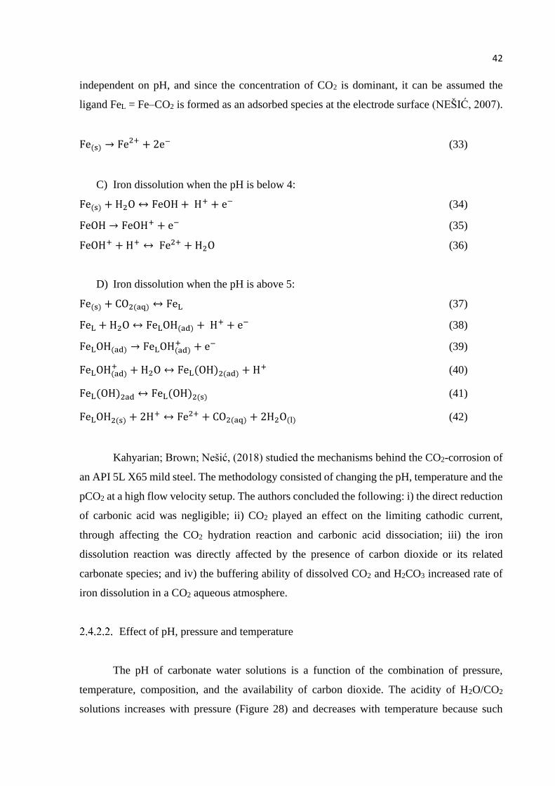
42

independent on pH, and since the concentration of CO2 is dominant, it can be assumed the

ligand FeL = Fe–CO2 is formed as an adsorbed species at the electrode surface (NEŠIĆ, 2007).

Fe(s) → Fe2+ + 2e− (33)

C) Iron dissolution when the pH is below 4:

Fe(s) + H2O ↔ FeOH + H+ + e− (34)

FeOH → FeOH+ + e− (35)

FeOH+ +H+ ↔ Fe2+ + H2O (36)

D) Iron dissolution when the pH is above 5:

Fe(s) + CO2(aq) ↔ FeL (37)

FeL + H2O ↔ FeLOH(ad) + H+ + e− (38)

FeLOH(ad) → FeLOH(ad)+ + e− (39)

FeLOH(ad)+ + H2O ↔ FeL(OH)2(ad) + H

+ (40)

FeL(OH)2ad ↔ FeL(OH)2(s) (41)

FeLOH2(s) + 2H+ ↔ Fe2+ + CO2(aq) + 2H2O(l) (42)

Kahyarian; Brown; Nešić, (2018) studied the mechanisms behind the CO2-corrosion of

an API 5L X65 mild steel. The methodology consisted of changing the pH, temperature and the

pCO2 at a high flow velocity setup. The authors concluded the following: i) the direct reduction

of carbonic acid was negligible; ii) CO2 played an effect on the limiting cathodic current,

through affecting the CO2 hydration reaction and carbonic acid dissociation; iii) the iron

dissolution reaction was directly affected by the presence of carbon dioxide or its related

carbonate species; and iv) the buffering ability of dissolved CO2 and H2CO3 increased rate of

iron dissolution in a CO2 aqueous atmosphere.

Effect of pH, pressure and temperature

The pH of carbonate water solutions is a function of the combination of pressure,

temperature, composition, and the availability of carbon dioxide. The acidity of H2O/CO2

solutions increases with pressure (Figure 28) and decreases with temperature because such

43

combination provides lower solubilities of carbonic acid (AQION, 2018; HANGX, 2005;

HENRY, 1803; OLI STUDIO, 2016).

Figure 28: Effect of increasing pressure on the pH of the water/CO2 solution at 25 °C.

Source: (SCHÜTZE; ISECKE; BENDER, 2011).

The intensity of the corrosion is a consequence of the atmospheric parameters. For

instance, it is known that acid brines tend to corrode faster than neutral or basic brines (see

Figure 29). The reason behind that is the fact that the acidity tends to intensify the cathodic

reactions. On the other hand, neutral or basic brines encourage low corrosion rates through the

inverse behaviour and favouring the formation of protective scales (ALMEIDA et al., 2017;

BARKER et al., 2018; HERNANDEZ; MUÑOZ; GENESCA, 2012; NEŠIĆ, 2007; SUN, 2006;

THU; BROWN; NEŠIĆ, 2015).

44

Figure 29: The effect of pH in the absence of iron carbonate scales on measured and predicted

corrosion rates. Test conditions: 20 °C, pCO2 = 1 atm, 1 m/s, cFe2+ < 2 ppm.

Source: (NEŠIĆ, 2007).

Moreover, though low temperatures tend to increase acidity and the solubility of CO2,

the temperature can also accelerate chemical and electrochemical processes. As a result, the

morphology of the surface, nature and characteristics of the corrosion remains dependent of this

variable. As such, various forms of corrosion, such as stress corrosion cracking, pitting or

crevices, may result from specific combinations of temperature with pressure, microstructure,

flow velocity, iron and oxygen contents. In the particular case of bulk CO2-corrosion, the

corrosion rates increase progressively until temperatures close to 70 and 90 °C. Beyond this

range, the corrosion rates reduce because of the formation of thicker layers of stable corrosion

scales. In the low-temperature range (0 to 20 °C) the mass transfer coefficient can diminish.

Figure 30 demonstrates the effect of the temperature and the partial pressure of CO2 on the

corrosion of an API X65 steel (BARKER et al., 2018; HAN et al., 2007; KERMANI;

MORSHED, 2003; LÓPEZ; PÉREZ; SIMISON, 2003; MITZITHRA; PAUL, 2016; NEŠIĆ;

POSTLETHWAITE; OLSEN, 1996; SCHMITT; HÖRSTEMEIER, 2006; SUN, 2006).

45

Figure 30: a) Effect of temperature on the corrosion of an API X65 steel at pH4 - LSV in 0.1M

NaCl solution with no CO2. b) Effect of pCO2 on the corrosion of an API X65 steel

at pH4 - LSV in 0.1M NaCl solution at 30 °C.

a)

b)

Source: (KAHYARIAN; BROWN; NEŠIĆ, 2018).

Effect of iron

Dugstad et al. (2015, 2018) studied the effect of iron in brine/CO2 systems. The authors

observed a decrease in the corrosion rates along with an increase in the pH. Models designed

for bulk corrosion confirm that adding iron to water shall increase the pH. Data of the pH in

CO2 environments concerning the saturation level with iron obtained from the models

employed in the literature are shown in Table 3.

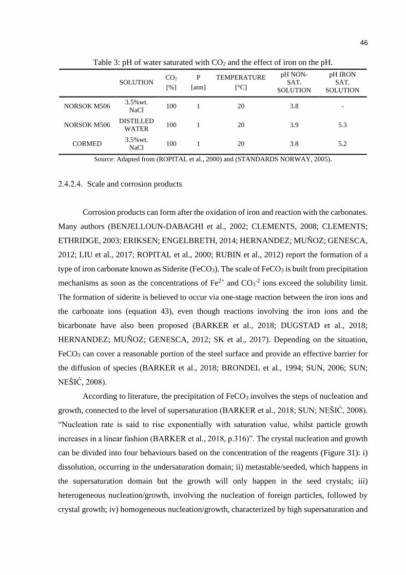
46

Table 3: pH of water saturated with CO2 and the effect of iron on the pH.

SOLUTION CO2

[%]

P

[atm]

TEMPERATURE

[°C]

pH NON-

SAT.

SOLUTION

pH IRON

SAT.

SOLUTION

NORSOK M506 3.5%wt.

NaCl 100 1 20 3.8 -

NORSOK M506 DISTILLED

WATER 100 1 20 3.9 5.3

CORMED 3.5%wt.

NaCl 100 1 20 3.8 5.2

Source: Adapted from (ROPITAL et al., 2000) and (STANDARDS NORWAY, 2005).

Scale and corrosion products

Corrosion products can form after the oxidation of iron and reaction with the carbonates.

Many authors (BENJELLOUN-DABAGHI et al., 2002; CLEMENTS, 2008; CLEMENTS;

ETHRIDGE, 2003; ERIKSEN; ENGELBRETH, 2014; HERNANDEZ; MUÑOZ; GENESCA,

2012; LIU et al., 2017; ROPITAL et al., 2000; RUBIN et al., 2012) report the formation of a

type of iron carbonate known as Siderite (FeCO3). The scale of FeCO3 is built from precipitation

mechanisms as soon as the concentrations of Fe2+ and CO3-2 ions exceed the solubility limit.

The formation of siderite is believed to occur via one-stage reaction between the iron ions and

the carbonate ions (equation 43), even though reactions involving the iron ions and the

bicarbonate have also been proposed (BARKER et al., 2018; DUGSTAD et al., 2018;

HERNANDEZ; MUÑOZ; GENESCA, 2012; SK et al., 2017). Depending on the situation,

FeCO3 can cover a reasonable portion of the steel surface and provide an effective barrier for

the diffusion of species (BARKER et al., 2018; BRONDEL et al., 1994; SUN, 2006; SUN;

NEŠIĆ, 2008).

According to literature, the precipitation of FeCO3 involves the steps of nucleation and

growth, connected to the level of supersaturation (BARKER et al., 2018; SUN; NEŠIĆ, 2008).

“Nucleation rate is said to rise exponentially with saturation value, whilst particle growth

increases in a linear fashion (BARKER et al., 2018, p.316)”. The crystal nucleation and growth

can be divided into four behaviours based on the concentration of the reagents (Figure 31): i)

dissolution, occurring in the undersaturation domain; ii) metastable/seeded, which happens in

the supersaturation domain but the growth will only happen in the seed crystals; iii)

heterogeneous nucleation/growth, involving the nucleation of foreign particles, followed by

crystal growth; iv) homogeneous nucleation/growth, characterized by high supersaturation and

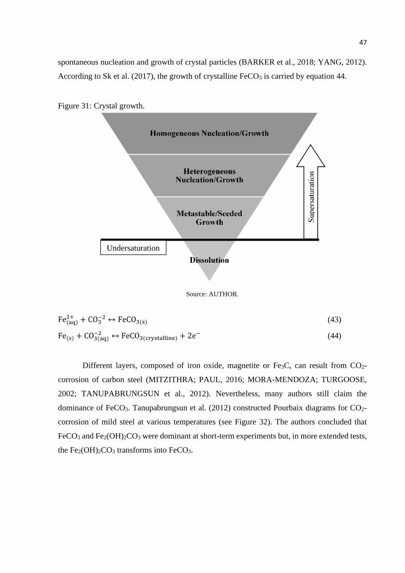
47

spontaneous nucleation and growth of crystal particles (BARKER et al., 2018; YANG, 2012).

According to Sk et al. (2017), the growth of crystalline FeCO3 is carried by equation 44.

Figure 31: Crystal growth.

Source: AUTHOR.

Fe(aq)2+ + CO3

−2 ↔ FeCO3(s) (43)

Fe(s) + CO3(aq)−2 ↔ FeCO3(crystalline) + 2e

− (44)

Different layers, composed of iron oxide, magnetite or Fe3C, can result from CO2-

corrosion of carbon steel (MITZITHRA; PAUL, 2016; MORA-MENDOZA; TURGOOSE,

2002; TANUPABRUNGSUN et al., 2012). Nevertheless, many authors still claim the

dominance of FeCO3. Tanupabrungsun et al. (2012) constructed Pourbaix diagrams for CO2-

corrosion of mild steel at various temperatures (see Figure 32). The authors concluded that

FeCO3 and Fe2(OH)2CO3 were dominant at short-term experiments but, in more extended tests,

the Fe2(OH)2CO3 transforms into FeCO3.

Undersaturation

48

Figure 32: Pourbaix diagrams for Fe-CO2-H2O systems at various temperatures (symbols: • -

bulk pH, ° - surface pH). a) 25 °C. b) 80 °C. c) 120 °C. d) 150 °C.

Source: (TANUPABRUNGSUN et al., 2012).

Effect of oxygen

In field applications, the structural layers of the pipe may experience corrosion with

certain amounts of oxygen, in unrepaired failures of the outer sheath for example. Oxygen acts

as a noxious chemical species that increases the corrosion rates, through enhancing the rate of

the cathodic reactions and, also, due to chemical destabilisation of the corrosion protective

scales that are stable in anaerobic conditions (LÓPEZ; PÉREZ; SIMISON, 2003).

Effect of calcium

Dugstad et al. (2015, 2018) studied how the calcium ions present in seawater may affect

the formation of FeCO3. The authors observed that calcium ions react to the dissolved

carbonates and form calcium carbonates (CaCO3). The kinetics of CaCO3 formation is faster

than the formation of FeCO3. Therefore, a considerable portion of carbonates can be consumed

a) b)

c) d)

49

when calcium ions are present, making the formation of FeCO3 more difficult. As a result, the

level of protection offered by FeCO3 can be compromised (BARKER et al., 2018).

Effect of the water flow velocity

Unrepaired failures expose the structural layer of the pipe to non-stagnant electrolytes,

that is to fluids colliding with the steel at given flow velocities. The impingement of the fluid

increases the corrosion rates by continuous erosion and dragging of the existing protective films

or through enhancing mass-transfer corrosion mechanisms near the surface of the steel. Beyond

erosion–corrosion, the flow velocity of the seawater can also trigger localised corrosion

mechanisms related to the mechanical destabilisation of passive scales (LÓPEZ; PÉREZ;

SIMISON, 2003).

Effect of the microstructure and chemical composition of the steel

The chemical composition and the microstructure of steels are known factors affecting

the CO2-corrosion. However, the accurate definition of their effective influence remains under

development, since conflicting results are found in the literature (BARKER et al., 2018;

KERMANI; MORSHED, 2003; LOPEZ et al., 2003; LÓPEZ; PÉREZ; SIMISON, 2003).

Despite the uncertainties, some aspects are worth mentioning, as follows:

i) Though it was not clearly determined the quantitative influence of the chemical

composition, heat treatment and microstructure, these factors clearly impact the

corrosion rates.

ii) A large number of recent studies indicate that ferritic-pearlitic microstructure

has better corrosion resistance than martensitic or martensitic-bainitic

microstructures.

iii) Microstructure and chemical composition interact with the stability, adherence

and distribution of carbides in the matrix.

iv) Additions of Cr, Mo, Cu, S and Ni to the composition of the carbon steel may

reduce the corrosion rates and corrosion tendency.

50

Annulus corrosion

Over the last decade, the study of the CO2-corrosion in unbounded flexible pipes has

gone through large developments as new cases of failure have been reported. Despite the efforts

of industry and academic community to understand the corrosion mechanisms, many

uncertainties remain, including those connected to the broad range of possible environmental

scenarios experienced by the flexible pipe concerning the annulus. Also, the annulus corrosion

of the structural wires is challenging because it not only requires knowledge of the common

aspects of bulk corrosion but also from the peculiarities of testing the materials in occluded

spaces. Many well-established electrochemical corrosion techniques become challenging to

employ, thanks to geometrical and chemical constraints (ERIKSEN; ENGELBRETH, 2014;

HERNANDEZ; MUÑOZ; GENESCA, 2012; LIU et al., 2017).

Previous studies shed light on the effect of the degree of occlusion on the corrosion rate,

i.e. the free volume (or volume of water) to steel surface area (V/S) present in the annulus.

According to the literature, degrees of occlusion ranging from 0.03 to 0.1 ml/cm² exist in

flexible pipes. The work to date shows that the corrosion rate decreases as V/S is reduced (see

Figure 33). The typical values for CO2-corrosion rates for such degree of occlusions lie below

0.01 mm/y. Besides the direct impact, the confinement can be a crucial factor due to its

influence on other variables such as pH, precipitation rate, stability of corrosion products and

etc. (4SUBSEA, 2013; CLEMENTS, 2008; CLEMENTS; ETHRIDGE, 2003; DUGSTAD et

al., 2015; ROGOWSKA et al., 2016; ROPITAL et al., 2000; RUBIN et al., 2012;

UNDERWOOD, 2002).

51

Figure 33: Corrosion rate as a function of the V/S ratio.

Source: (CLEMENTS, 2008).

Ke et al. (2017) studied the combination of confinement and pressure on the evolution

of pH at ambient temperature. The authors observed an increase in pH to a peak before

stabilising (see Figure 34). This behaviour was attributed to the rise in concentrations of iron

ions and bicarbonate. The works of Dugstad et al. (2015, 2018) seem in line with this statement

as they show an increase in pH when the concentration of iron ions in the solution was

artificially raised.

52

Figure 34: Long-term evolution of pH measured in a confined test cell at ambient

temperature, under 1 to 45 bar (44,4 atm) of CO2.

Source: (KE et al., 2017).

When the concentrations of iron ions exceed the solubility limit, mineral forms of iron

carbonate can form, by precipitation mechanisms, adhering on the surface of the structural

layers of the pipe. Once the precipitation rate exceeds the corrosion rate, the scale formed on

the surface of the steel is considered as protective (NEŠIĆ, 2007; SUN, 2006; SUN; NEŠIĆ,

2008). Sun and Nešić (2018) deduced equation 45 that describes the rate of precipitation

(PRFeCO3) in mol/m³s when all of the ferrous ions end up on the steel surface. It can be observed

that PRFeCO3 is a function of the concentrations of iron (cFe) and carbonate (cCO32-), of the

supersaturation level of FeCO3 (SSFeCO3, see equation 46), of the temperature (T), of the degree

of occlusion (V/S), of the solubility limit (Ksp, see equation 47), of the kinetic constant (Kr, see

equation 48) and of the constants “C3”, “C4” and “R”, described in the literature (KE et al.,

2017; NEŠIĆ, 2007; SUN, 2006; SUN; NEŠIĆ, 2008). It can be noticed that the precipitation

rate of FeCO3 increases when the degree of occlusion is reduced. Besides that, the atmospheric

conditions can also affect the precipitation rate of FeCO3 directly through an impact on the

solubility limits of chemical species in the solution (AQION, 2018; BARKER et al., 2018;

HANGX, 2005; HENRY, 1803; OLI STUDIO, 2016).

53

PRFeCO3 = KrKsp

V S⁄(SSFeCO3 − 1) (45)

SSFeCO3 =cFe2+

×cCO32−

Ksp (46)

logKsp = −59.3498 − 0.041377T − 2.1963 T⁄ + 24.5724 log(T ) + 2.518I0.5 − 0.657I

(47)

Kr = eC3−

C4

RT (48)

Since the protective precipitates tend to adhere on the surface of the steel, it becomes

interesting to explore the effect of the coverage of the surface by the action of a protective scale,

such as FeCO3. Remita (2008) modelled the impact of the coverage aspect (θ) on the surface of

steel in brines at 1 atm of carbon dioxide. The authors concluded that a considerable reduction

of the corrosion rate and pH should occur when more insulating scales cover the surface; see

Figure 35 and Figure 36. Furthermore, it is reasonable to assume that the magnitude of θ could

grow over time, as continuous layers of precipitates accumulate on the surface of the steel. The

effect of time was also covered in the work of Clements (2008), where the author observes a

reduction of the corrosion rate with time (see Figure 37).

Figure 35: Corrosion rate as a function of the V/S ratio for different θ at pCO2 = 1 atm and

20 °C.

Source: (REMITA et al., 2008) and (ROPITAL et al., 2000).

54

Figure 36: pH as a function of the V/S ratio for different θ; at pCO2 = 1 atm and 20 °C.

Source: (REMITA et al., 2008) and (ROPITAL et al., 2000).

Figure 37: Annulus corrosion rate from weight loss measurements of specimens in CO2

saturated deionised water at 50 °C.

Source: (CLEMENTS, 2008).

Despite the factors intimately tied to the degree of occlusion, a massive effort was

dedicated over the last decades to explore CO2-corrosion in terms of mechanisms, morphology

and corrosion products (ALMEIDA et al., 2017; BARKER et al., 2018; CROLET;

THEVENOT; NEŠIĆ, 1998; HAN et al., 2007; MORA-MENDOZA; TURGOOSE, 2002;

SCHMITT; HÖRSTEMEIER, 2006; SUHOR et al., 2012; SUN, 2006; SUN; NEŠIĆ, 2008;

55

TANUPABRUNGSUN et al., 2012), temperature and environmental aspects, (ALMEIDA et

al., 2017; BARKER et al., 2018; MITZITHRA; PAUL, 2016; ROSLI et al., 2016)

microstructure and chemical composition of the steel, (BARKER et al., 2018; LIU et al., 2016;

LOPEZ et al., 2003; LÓPEZ; PÉREZ; SIMISON, 2003) properties and characteristics of the

electrolyte (BARKER et al., 2018; DUGSTAD et al., 2015, 2018; FANG; BROWN; NEŠIĆ,

2013; ZENG; LILLARD; CONG, 2016). However, little information was found concerning the

effect of CO2 flow rates. Many studies do not state the flow rates or the surface area of steel,

making it difficult to compare data regarding the relative flow rates.

As the flow rate of carbon dioxide into the annulus is primarily controlled by the

permeability of the polymer sheath containing the bore fluid, and that permeability will vary

depending on the polymer structure and its thickness, it seems that flow rate is a variable worth

exploring. Most standard corrosion tests would employ relatively high flow rates in order to

obtain saturated solutions from the beginning of a test, which contrasts with the relatively slow

establishment of the annulus conditions evolving in service through diffusion of molecules

through the inner polymer sheath (DÉSAMAIS; TARAVEL-CONDAT, 2009; HAAHR et al.,

2016; KE et al., 2017).

Moreover, in the event of a breach of the outer sheath, seawater ingress the annulus at

hydrostatic pressure and temperature respective to the depth of the failure. A recent failure of a

flexible pipe operating as a CO2 injection line in Brazil confirms the existence of different forms

of corrosion other than uniform corrosion. This particular failure brought the attention of the

oil and gas community to the possible deterioration of tensile wires by stress-corrosion cracking

(SCC), in pipes operating with high concentrations of carbon dioxide (CHETWYND, 2017).

The mechanisms of SCC in flexibles remains under investigation, but according to Schmitt and

Hörstemeier (2006), the susceptibility of high strength carbon steel to SCC in CO2 wet

environments increases with the partial pressure of carbon dioxide, temperatures and applied

mechanical loads.

The work of Borges (2017) reveals the possibility of localised CO2-corrosion in the

tensile wires on a real-scale test. The occurrence of pits in CO2-containing environments is

associated by Han et al. (2007) with moderate iron carbonate supersaturation, which seems in

line with the results shown by Borges (2017).

The phenomenon of pitting in wet CO2 divides into two stages: initiation and growth.

The initiation is related to a chemical removal or mechanical breakdown of a protective scale

of FeCO3 (HAN et al., 2007). Brondel et al. (1994) link the occurrence of pitting and crevice

with the contact of the surface of the steel with carbonic acid. Mitzithra and Paul (2016) studied

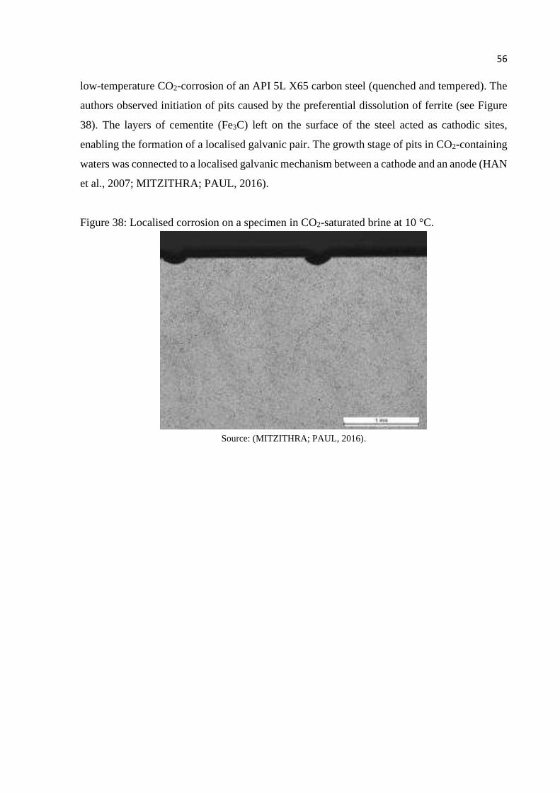
56

low-temperature CO2-corrosion of an API 5L X65 carbon steel (quenched and tempered). The

authors observed initiation of pits caused by the preferential dissolution of ferrite (see Figure

38). The layers of cementite (Fe3C) left on the surface of the steel acted as cathodic sites,

enabling the formation of a localised galvanic pair. The growth stage of pits in CO2-containing

waters was connected to a localised galvanic mechanism between a cathode and an anode (HAN

et al., 2007; MITZITHRA; PAUL, 2016).

Figure 38: Localised corrosion on a specimen in CO2-saturated brine at 10 °C.

Source: (MITZITHRA; PAUL, 2016).

57

3. MATERIALS AND METHODS

3.1. ORGANISATIONAL CHART

Figure 39 shows an organisational chart presenting the methodology of the work,

divided into three categories: general simulations, laboratory experiments and exploration of

environmental aspects. The laboratory experiments were conducted according to the results

provided by the general simulations. The software packages were not only used to reproduce

and enhance the quality of the experimental results but also to search for more critical corrosion

patterns and to reduce the gaps of knowledge linked to the environmental conditions of the

water solution.

Figure 39: Organisational chart.

Source: AUTHOR.

58

3.2. GENERAL SIMULATIONS

Carbon dioxide flow rate calculations

The flow rate of CO2 per surface of the steel (FR/SS) was selected as a controlled

parameter used to reproduce the process of permeation happening in the annulus. The term flow

rate is used throughout this work to represent the flow rate per square centimetres of steel. The

value employed in the reproduction of the annulus CO2-corrosion derived from the outcome of

software developed to predict the annulus environment. An additional experiment conducted

with a flow rate augmented by a factor of 100 times was performed to study the influence of

the parameter FR/SS on the corrosion process. The software employed models the pipe

structure, service conditions and calculates the flux and partial pressure of the gases in the

annulus. It is recognised that substantial efforts are currently being dedicated to improving the

precision of the models available designed to the assessment of the permeation rates of gases

entering the annulus. However, it should be highlighted that the software used here consisted

of the best tool available at the given moment. Further details regarding the name of the software

and polymer grades employed are kept confidential.

Five input conditions representative of extreme CO2 service were simulated. The

parameters ranged as follows: pressures in the bore ranging from 300 to 800 bar (296,077 to

789.5 atm); temperatures ranging from 60 to 80 °C; surfaces per length of 330 cm²/cmlength and

531 cm²/cmlength; and three different polymer grades, which are relevant to the structures

employed in the field. Information about the exact type of polymer grade employed was

suppressed, due to confidentiality constraints.

Commercial software packages

The state and the characteristics of 3.5%wt. NaCl solution was simulated with the help

of two commercial models: OLI Studio™ and Aqion™. Both software packages are suited to

simulate equilibrium reactions, ion exchanges, surface complexes, solid solutions and gases.

They were used in a complementary manner, as different databanks and modelling strategies

are employed.

OLI Studio™ can work with two databanks: Aqueous Phase (AQ) and Mixed Solvent

Electrolyte (MSE). AQ was selected, as it is well suited to the environment examined in the

experiments; the validity ranges are displayed in Table 4.

59

Table 4: Validity range of the software OLI Studio™.

Databank/model: Aq (Aqueous Phase)

Chemicals: Aqueous electrolytes (XH2O > 0.65)

Ionic strength (mol/mol): 0 < I < 30

Pressure range (atm): 0 to 1480

Temperature range (°C): -50 to ~300

Source: (OLI STUDIO, 2016).

Aqion™ is a model inspired by the geochemical model PHREEQC. The environment

is modelled by the common activity model, which is calculated either by equation 49 (also

known as Davies equation) or by equation 50 (also known as WATEQ Debye-Hückel equation).

The term “γ±” are activity coefficients, “IS” is the ionic strength, “zj” is the valence of ion “j”,

“aj0” and “bj” are ion-specific parameters. “C1” and “C2” are variables depending on

temperature. The validity range of the models is defined by the ionic strength, limited to values

below 1M.

logγ± = −C1zj2 (

√IS

1+√IS− 0.3IS) , IS ≤ 0.5M (49)

logγ± = −C1zj2 (

√IS

1+C2aj0√IS) + IS ∙ bj, IS < 1M (50)

Boundaries and assumptions for the reproduction of the experimental results

It is assumed the possibility of two main boundary conditions: open and closed

carbonate systems. As detailed in the literature review, the difference between them lies in the

fact that closed carbonate system does not allow the exchange of matter with the

neighbourhood, whereas open carbonate system does. Figure 40 shows a sketch, presenting the

main assumptions of the system (annulus) and its neighbourhood. Simulations of titrations are

used to highlight the differences between boundaries. The simulation of the titration involves

modelling additions of NaOH or HCl into the solution, in order to alter the pH and the

composition. The chemical species of interest were: hydrogen ions, carbonic acid, bicarbonate

and carbonate. It is assumed that carbon dioxide undergoes slight hydration (~ 0.26 %) to

H2CO3, and that usual analytical methods do not clearly distinguish between the dissolved

carbon dioxide and the carbonic acid. Hence, these chemicals are represented as one

component, described by the term “CO2(aq)”. Such a convention is used and supported elsewhere

(AQION, 2018; KORDAČ; LINEK, 2008; OLI STUDIO, 2016).

60

Figure 40: Main interactions between the system and the neighbourhood. a) Open carbonate

system and b) Closed carbonate system.

Source: AUTHOR.

The data obtained in the laboratory were used for validation of the models and

boundaries. Based on the experimental outcomes, the simulation assumed that under various

atmospheric conditions the high strength steel tensile wires should corrode and release iron ions

in the annulus. The concentration of iron can evolve towards the supersaturation domain,

eventually causing pH variations and precipitation of corrosion products. Beyond this stage, the

concentration of iron should return toward the saturation level or close. The formation of FeCO3

as the protective scale has been presumed because many authors support its dominance in pure

CO2-corrosion. Nonetheless, a confirmation of such a scale was carried by X-ray diffraction

(XRD) (BARKER et al., 2018; DUGSTAD et al., 2015, 2018; HERNANDEZ; MUÑOZ;

GENESCA, 2012; KE et al., 2017; NEŠIĆ, 2007; RUBIN et al., 2012; SUN, 2006;

TANUPABRUNGSUN et al., 2012).

3.3. LABORATORY EXPERIMENTS

Material

High strength steel tensile wires, taken from the first and second tensile layer of a water

injection jumper, were used in this work. The alloy is of interest for service in deep wells,

because it offers high strength to weight ratio. Thus, it is suited to supporting the high loads

imposed in deep-water developments. The wires have nominal UTS higher than 1400 MPa. The

main strengthening alloy element was carbon, at the content of 0.68% in weight. Further details

regarding microstructure, hardness and chemical composition were suppressed due to

confidentiality constraints.

a) b)

CO2

61

Experimental matrix

Table 5 summarises the experimental conditions investigated. The tests were conducted

at 30±2 °C and atmospheric pressure, with a carefully controlled flow rate of CO2. The

simulation of flux due to permeation was the basis for the magnitude of the flow rate of CO2

per surface of steel used in laboratory experiments. A flow rate of 0.0008 ml.min-1.cm-2 was

selected for the reproduction annulus corrosion (experiment No 1). This flow rate is considered

close to the values obtained by simulations of the permeation rates at critical CO2 operating

conditions, as well as being practically achievable in the laboratory.

The literature suggests that a higher flow rate could alter the state and time to establish

steady-conditions. Therefore, one additional short-term experiment (experiment No 2) was

carried at the FR/SS of 0.0785 ml.min-1.cm-2. Such a magnitude was selected to ensure a

significant difference in the variable being examined and to represent something closer to what

would be used in a more typical corrosion experiment.

Table 5: Summary of the corrosion tests carried out in 3.5 %wt. NaCl solution. The matrix

presents the following parameters: flow rate of CO2 per unit surface of steel (FR/SS), degree

of occlusion (V/S), pressure, type of gas, temperature and time.

No

FR/SS V/S Pressure

[atm]

Gas Temp. Time

[ml/min/cm2] [ml/cm2] type [°C] [Months]

1 0.0008 ~0.2 1 CO2 30±2 4

2 0.0785 ~0.2 1 CO2 30±2 2

Test details

The test vessel comprised of 500 ml cylindrical glassware, each containing

simultaneously 52 high strength steel tensile wires and around 260 ml of brine. From the total

of samples in each experiment, 2 samples are used for the electrochemical measurements (WE1

and WE2). The remaining material is used as steel coupons and for surface characterization.

The surface preparation for all samples involved submersion in Clarke`s reagent (3

cycles of 15 minutes each) at ambient temperature to remove surface oxides (AMERICAN

SOCIETY FOR TESTING AND MATERIALS, 2003). The test solution was 3.5 %wt. NaCl,

prepared by the addition of high-grade reagent to de-ionised water. Deaeration was performed

prior to the introduction of water into the glass test vessel and the introduction of carbon

dioxide. The oxygen concentration was reduced to values below 10 ppb using nitrogen purging

62

before transfer into the pre-purged vessel, in order to avoid preferential corrosion by dissolved

oxygen. After deaeration and transfer of the test solution, CO2 (99.995%) was introduced at the

intended flow rate. At the end of the test, all samples were immediately dried, placed in a

desiccator and filled with N2 to avoid atmospheric corrosion.

Environment monitoring

Measurements of pH and iron in solution were monitored on a regular basis over the

duration of the tests. A special modification to the setup of the glass test vessel allowed the

measurement of pH and the sampling of iron ions in solution with minimal disturbance of the

test environment (see Figure 41). Both the pH and iron measurements were performed forcing

the passage of the solution contained in the lower part of the test cell through the same piping

used for gas inlet. This procedure was performed to improve the representativeness of the

analysed solution and to prevent the measurement of solutions stagnant in the pipe, which

would not be representative of the test. Another advantage of the setup used in this work was

that it is not necessary to keep the gauge used to measure pH permanently connected to the test

cell. This allowed calibration before every measurement without the risk of disturbing the test

environment.

The most significant changes in behaviour were expected to take place in the initial

stages of the test. Hence, a higher frequency of sampling was performed at the beginning and

was reduced throughout the experiment, as more stable conditions developed. Also, the volume

of each aliquot removed for measurement of iron (2.5 ml) was minimised to prevent any

significant change to the degree of occlusion. It is expected that the total change in the degree

of occlusion, due to the aliquots would lie below 0.03 ml/cm². In the literature, the concentration

of iron is frequently presented in mg/l, instead of mol/l, so the first unit is preferred in this work

to describe the evolution of iron concentration. The latter unit (mol/l) is used for the other

chemicals in the solution due to practicality concerning simulation.

63

Figure 41: a) Glass test vessel. b) Water sampling for iron ions.

Source: AUTHOR.

Electrochemistry

The electrochemical analyses were conducted with a three-electrode electrochemical

setup and an Ivium Vertex potentiostat/galvanostat. Each glass vessel contained two samples

selected as working electrodes (WE1 and WE2), one platinised titanium counter electrode (CE),

and one reference electrode of Ag/AgCl (RE), connected to the test solution by a commercial

polymer salt bridge. Figure 41 and Figure 42 show the careful arrangement of the

electrochemical specimens. The electrodes, thermocouple, the salt bridge and the coupons were

all positioned vertically in the glass vessel. The CE and the salt bridge were placed between the

working electrodes.

The areas of the working electrodes wire samples were measured with the software

Image J and ranged from 0.808 to 0.903 cm². The remaining surface area was covered with a

lacquer to prevent corrosion and electric contact from the other wires confined in the vessel.

This step was critical for obtaining reliable electrochemical data.

a) b) Sampling port

WE1,2

RE

CE

64

Figure 42: Scheme of the electrode layout for an electrochemical test in the occluded

environment. The detail shows the steel surface and the anti-corrosion lacquer used

to define it.

Source: AUTHOR.

The electrochemical techniques employed in this work were open circuit potential

(OCP), linear polarisation resistance (LPR) and linear sweep voltammetry (LSV).

LPR is a non-destructive technique designed for rapid real-time corrosion monitoring.

The linear polarisation resistance analysis employed a range of -10 mV to +10 mV from OCP,

at a scan rate of 1 mV/s. The corrosion rates were calculated using equations 51 to 54 according

to ASTM G59-97. The term “jcorr” is the corrosion current density, “B” is the Stern-Geary

factor, “Rp” is the polarisation resistance, “E” is the potential, “i” is the current density, “ba”

and “bc” are anodic and cathodic Tafel slopes, “CRLPR” is the corrosion rate given by LPR in

mm/y, “EW” is equivalent weight of the steel, “ρ” is the density of the steel (AMERICAN

SOCIETY FOR METALS INTERNATIONAL, 2003; AMERICAN SOCIETY FOR

TESTING AND MATERIALS, 1989, 1997; DENZINE; READING, 1997; PEREZ, 2004;

ROBERGE, 2000; WOLYNEC, 2003). As well as occurred with the environment monitoring,

a higher frequency of testing was performed at the beginning and was reduced throughout the

experiment, as more stable conditions developed. Nevertheless, it can be said that at least three

LPR measurements/week were carried at each flow rate condition during most of the tests

durations.

WE1

WE2

CE

STEEL SURFACE ON

THE CONCAVE SIDE OF

THE SPECIMEN

LACQUER

65

jcorr =B

Rp (51)

Rp = (∂Ԑ

∂j)j=0, dE/dt→0

(52)

B =babc

2.303(ba+bc) (53)

CRLPR = 3.27 × 10−3 jcorr EW

ρ (54)

The primary cause of inaccuracies associated with LPR is the use of an incorrect Stern-

Geary factor (B). In an effort to minimise the inaccuracies, B was obtained from the slopes (ba

and bc) derived from the final linear sweep voltammetry (LSV) at the end of the four months

test at a FR/SS of 0.0008 ml.min-1.cm-2. Rogowska et al. (2016) observed B varying from 20 to

27 mV, based on results of weight loss.

The linear sweep voltammetry consists of sweeping the potential of the working

electrode at several hundred millivolts more than those applied to the LPR technique. The

broader range of the sweep facilitates the determination of accurate slopes (ba and bc) and

corrosion rates. The LSV destroys the surface of the sample, and thus the analyses were only

performed at the end of each experiment. The potential sweep ranged from –300 to +300 mV

with respect to the OCP. The sweep was conducted at a scan rate of 1 mV/s (AMERICAN

SOCIETY FOR METALS INTERNATIONAL, 2003; AMERICAN SOCIETY FOR

TESTING AND MATERIALS, 2014a, 2014c; DENZINE; READING, 1997; PEREZ, 2004;

ROBERGE, 2000; WOLYNEC, 2003).

Weight change techniques

Weight loss and weight gain are frequent and reliable methods used to obtain average

corrosion rates and scales growth respectively. The measurements were carried out based on

procedures described in the literature and ASTM G1-03 (AMERICAN SOCIETY FOR

TESTING AND MATERIALS, 2003; SUN, 2006). A total of 46 tensile wires (70 mm x 12

mm x 5 mm) were weighed per test condition. The remaining samples were used for surface

examination and electrochemical tests. As recommended by ASTM G1-03, repeated cycles of

submersion in Clarke`s reagent were made to remove the corrosion scale (AMERICAN

SOCIETY FOR TESTING AND MATERIALS, 2003).

The average corrosion rate (ACR) was obtained by equation 55 (in mm/y), or by

equation 56 (in mol/(m²h)). The average scale growth (ASG) was calculated by equation 57 (in

66

mol/(m²h)). Note that ASG does not comprehend the scale adhered in the glass vessel. Sun

(2006) shows that the incertainties related to the adherence of scale in the test vessel decrease

when V/S becomes smaller. The term “m1” is the initial weight of the coupon (g); “m2” is the

weight of coupon after the end of the test (g); “m3” is the weight of coupon after complete

removal of the corrosion scale (g). “MWFeCO3” is the molecular weight of iron carbonate

(g/mol). “t” is the time (hours). “S” is the surface area of the steel (m²). “ρ” is the density of the

steel (kg/m³).

ACR =m1−m3

MWFe×t×S×365×24×MWFe

ρ (55)

ACR =m1−m3

MWFe×t×S (56)

ASG =m2−m3

MWFeCO3×t×S (57)

The preferential formation of FeCO3 was assumed in equation 57, grounded by its

dominance in similar CO2 environments, which is supported by many authors (BARKER et al.,

2018; DUGSTAD et al., 2015, 2018; HERNANDEZ; MUÑOZ; GENESCA, 2012; KE et al.,

2017; NEŠIĆ, 2007; RUBIN et al., 2012; SUN, 2006; TANUPABRUNGSUN et al., 2012). A

clear identification of the corrosion scale was carried by X-ray diffraction (XRD), improving

the level of certainty of the weight gain results.

Statistical analysis

The statistical treatment performed in this work involved the collection and careful

scrutinisation of quantitative data of ACR and ASG to obtain statistically relevant data.

Sample size

A choice of sample size for estimation is calculated from equation 58. The minimum

sample size achieved for each experiment was 46 specimens, with a confidence level of 95%,

a standard deviation of 0.005 mm/y and a margin of error of 0.0015 mm/y. While the margin

of error (e) could be chosen by experience, the standard deviation (Sd) was estimated by the

calculus of Sd from the data of average corrosion rates available in the work of Rubin, A. et al.

(2012). Their dense packed experiment, with a V/S of 0.17 ml/cm², was carried over 1464 hours

67

in artificial seawater, deaerated overnight and saturated with carbon dioxide aqueous solution

at 23 °C. Information in the literature to allow an estimation of Sd for weight gain concerning

ASG was not found, so the sample size used in this work concerns the average corrosion rates

only.

n = (Zα/2.Sd

e)2

(58)

Outliers

Given the considerable number of samples and the complexity of the tests, the statistical

analyses considered the possibility of outliers, defined by the abnormal distances from others

in a random sample of a population. The methods to exclude the samples from the analysis was

the Inter Quartile Range (IQR) and the modified Thompson Tau Test.

Tolerance interval

The tolerance interval provides a range of values of average corrosion rates and average

scale growth that likely covers a proportion of the population. In other words, the tolerance

specifies a proportion of the population at a specified confidence level. The calculation was

performed using the software Minitab 17, which calculates the tolerance using either the

Normal or Nonparametric Methods. The normal tolerance method is employed when the data

follow a normal distribution, whereas the nonparametric tolerance method is used when the

probability distribution is non-normal. The non-normal method is advantageous when the data

cannot be transformed into normal by applying transformations functions, such as box-cox or

Johnson transformations. Further details and equations used by the statistical software can be

found in the software Minitab 17 or in the literature (CHOU; POLANSKY; MASON, 1998;

DE MIRANDA, 2005; KRISHNAMOORTHY; MATHEW, 2009; ODEH, 1978; OLDONI;

RIBEIRO; WERNER, 2015)

Scaling tendency

The thickness of the scale layer should not be interpreted as a definite indication of the

protectiveness of the corrosion product, once the density and adhesion shall also be accounted.

68

Accordingly, a non-dimensional parameter called scaling tendency (ST) can be used to

characterise the kinetics of the formation of scales in CO2-corrosion (BARKER et al., 2018).

ST is calculated by the ratio between ASG and ACR using the same molar units, equation 59.

If ST exceeds a given critical value, the corrosion scale can be assumed as protective; otherwise,

an unprotective film is likely to form. Figure 43 shows a guideline for the critical scaling

tendencies as a function of microstructure and chemical composition of the steel (VAN

HUNNIK; POTS; HENDRIKSEN, 1996). The plot does not comprehend the carbon content of

the HSS used in this work. However, if the general trend is kept unaffected, it is reasonable to

assume that the critical ST would tend to decrease to values below 90% by further increase of

the carbon content.

ST =ASG

ACR (59)

Figure 43: Critical scaling tendencies at which protective corrosion scale begins to form in CO2-

corrosion.

Source: Adapted from (VAN HUNNIK; POTS; HENDRIKSEN, 1996).

Characterisation of the corrosion surface

The corrosion surface of the HSS tensile wires was studied with light and scanning

electron microscopy (SEM). A definitive characterisation of the corrosion product was obtained

by X-ray diffraction (XRD) analysis.

Carbon content (wt%)

69

3.4. EFFECT OF THE ATMOSPHERIC VARIABLES

The effects of the atmospheric variables on CO2-containing brines

Pressure and temperature in H2O/CO2 environments have been extensively explored

over the years. Nevertheless, this subject remains vital to considerations regarding the initial

states and compositions of the electrolytes confined in the annulus of unbounded flexible risers.

Hence, hydrochemistry models were used to simulate the impact of the atmospheric variables

on the properties and composition of a 3.5%wt. NaCl brine. A wide range of pressures and

temperatures was proposed to cover liquid, gaseous and supercritical states of carbon dioxide

(see Table 6). It is plausible that the tensile wires could be in contact to cold seawater in case

of unrepaired failures at large depths, so the lowest temperature considered was 5 °C (SCRIPPS

INSTITUTION OF OCEANOGRAPHY, 2013).

Table 6: Range of the variables considered to the simulation.

Pressure range (atm) 1– 90

Temperature range (°C) 5 – 90

Aqueous Solution composition 3.5%wt. NaCl

Aqueous Solution Volume @ 1 atm (L) 1.0

Aqueous Solution (mol) 55.9644

Gas phase/Mole fraction (%) CO2/100

Annulus environment – concentration of iron

The state and composition of the electrolyte are critical factors for the occluded CO2-

corrosion. Thus, simulations were carried to investigate a 3.5%wt. NaCl brine saturated with

carbon dioxide and containing different amounts of iron. Table 7 shows the range of pressure

and temperatures investigated. In each environmental combination, the concentration of iron in

the solution was varied, covering the undersaturation, the saturation and the supersaturation

domains of iron. The findings from this work and the literature were used as a criterion for the

magnitudes and the likely consequences.

Hence, this section aims at searching for more critical corrosion patterns and on

providing guidelines for further experimental annulus testing. It does not provide a holistic view

of the corrosion process, as the flexible risers technology is young and unknown factors may

exist. However, at this stage, it was impractical to consider a more extensive number of

variables because additional and laborious laboratory investigations would be required.

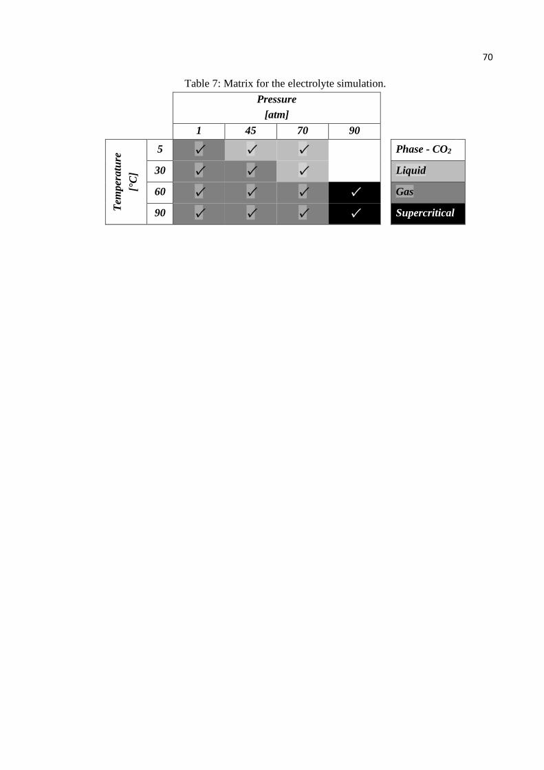
70

Table 7: Matrix for the electrolyte simulation.

Pressure

[atm]

1 45 70 90

Tem

per

atu

re

[°C

]

5 ✓ ✓ ✓ Phase - CO2

30 ✓ ✓ ✓ Liquid

60 ✓ ✓ ✓ ✓ Gas

90 ✓ ✓ ✓ ✓ Supercritical

71

4. RESULTS AND DISCUSSION

4.1. CARBON DIOXIDE FLOW RATES

An analysis of the permeation of carbon dioxide in the typical polymer grades relevant

to the structures employed in the field was carried to obtain a representative range of flow rates

to be used in laboratory experiments. Table 8 shows the results of the permeation analyses, the

flow rate per square cm of steel is presented for the different bore conditions.

Table 8: Results of the CO2 permeation analyses.

No. Press. Temp. Polymer Type Surface per length

Permeation rate per

surface of the steel

bar/atm Int.[°C] Ext.[°C] Inner sheath cm2/cmlength ml/min/cm2

1 800/790 80 10 A 531 0.00043

2 800/790 80 10 A 330 0.00034

3 800/790 80 10 B 531 0.00010

4 800/790 80 10 C 531 0.00376

5 300/296 60 5 C 531 0.00065

Based on the results, a wide range of flow rates could be employed in the laboratory

experiments, given that the lowest permeation rate was 0.00010 ml.min-1.cm-2 (analysis No. 3)

and the highest was 0.00376 ml.min-1.cm-2 (analysis No. 4). Comparing analysis No. 3 and No.

4, the simulation indicates that there is a significant difference between the permeation rates

obtained for different polymers with the same bore conditions. Therefore, the analyses highlight

the importance that the inner sheath plays in controlling carbon dioxide permeation into the

annulus. Also, pressure, temperature and geometry of the pipe affected the permeation, where

the combination of higher pressures and temperatures increased the carbon dioxide flow rate

into the annulus as shown by a comparison between analysis No. 4 and No. 5.

4.2. PROPERTIES OF THE OCCLUDED ELECTROLYTES

Experimental evolutions of the occluded electrolyte

The concentration of iron ions was monitored regularly throughout the tests. Figure 44

shows the evolution of iron concentration (solid line) and pH (dotted line) over time, alongside

the simulated saturation of iron in 3.5%wt. NaCl brine (horizontal dashed line). The achieved

72

simulated solubility limit of Fe2+ was 186 mg/l (3.34 mM), at 1 atmosphere of CO2 and 30±2 °C.

This value is close to values found in the literature (ROGOWSKA et al., 2016).

Figure 44: Concentration of iron ions in the solution over time. The saturation with iron ions

was simulated under the environmental conditions tested in the laboratory. Test

conditions: V/S of 0.2 ml/cm², 3.5%wt. NaCl brine, FR/SS of 0.0008 ml.min-1.cm-2,

1 atm of CO2 and 30±2 °C.

Source: AUTHOR.

The plot shows that the occluded environment is reasonably sensitive to the release of

iron ions caused by the corrosive processes. Apart from the initial measurements (after nitrogen

purging), no value below the calculated saturation of iron was measured. The solution remained

supersaturated with iron for the test duration, revealing the slow kinetics of precipitation. Only

at the end of the test does the iron concentration approach the steady-state at the saturation level

predicted by simulation. The maximum concentration of iron measured was 1165.2 mg/l,

observed after 359 hours, being around six times larger than the simulated saturation of iron in

the 3.5%wt. NaCl brine. Such concentration with iron is comparable to the data presented in

the literature (DUGSTAD et al., 2015, 2018; ROGOWSKA et al., 2016). The evolution of the

pH shows small variations, but on the whole remained close to pH6 for most of the test period.

The maximum value of pH6.15 was reached after 359 hours. The trends in pH mirrored the

timescales for the evolution in dissolved iron.

The pH of water in 1 atmosphere of CO2 is usually close to pH3.8. However, this was

not observed. The pH remained more basic due to the presence of iron and carbonates in the

73

solution and the electrochemical corrosion process. Figure 45 shows the correlation between

the concentration of iron and pH. The plot shows an increase in the pH as the concentration of

iron increase, the trend is shown by the black arrow. The pH follows the concentration of iron

as a direct consequence of the concentration of carbonates within the solution (DUGSTAD et

al., 2015, 2018; KE et al., 2017; ROGOWSKA et al., 2016). According to Ke, et al. (2017) the

pH of the solution changes with the reduction of H+ (equation 29) and the release of iron ions

and bicarbonate (see equation 60). Works in the literature suggest that the reduction of hydrogen

is the dominant cathodic reaction in a mechanism called buffering effect, driving the hydrogen

ions into gaseous H2(g), which can bubble out of the solution (ALMEIDA et al., 2017; THU;

BROWN; NEŠIĆ, 2015). The release of electrons due to the dissolution of iron, therefore,

disturbs the balance of the solution, removing hydrogen ions from solution and increasing the

relative quantity of carbonates.

H+ + e− ↔ 1 2⁄ H2(g) (29)

Fe + 2H2CO3 → Fe2+ + 2HCO3

− + H2 (60)

Figure 45: pH as a function of the iron concentration in the solution. Test conditions: V/S of

0.2 ml/cm², 3.5%wt. NaCl brine, FR/SS of 0.0008 ml.min-1.cm-2, 1 atm of CO2 and

30±2 °C.

Source: AUTHOR.

Simulations of the occluded electrolyte

Understanding the differences between the available boundaries of H2O/CO2 systems is

a fundamental step before the simulation of the occluded environment. The incorrect selection

74

of the interactions between the system and the neighbourhood yields misleading interpretations

of the aggressiveness of the solution and formation of corrosion products. Thus, simulations of

titration procedures were carried out to observe the main differences in the composition of

brines concerning variations of pH. The procedure involves virtual additions of HCl and NaOH

to cause variations in pH of a 3.5%wt. NaCl brine saturated with carbon dioxide. The pressure

and the temperature of the solution were selected to match those used in the laboratory

experiments. Furthermore, to observe the effect of the different boundaries on comparable

scenarios, the initial DICs of the CO2 saturated brines were kept identical for both scenarios.

Figure 46 shows the behaviour of an open aqueous carbonate system at atmospheric

pressure. It can be observed that the DIC changes according to variations in the pH, but the

concentration of carbonic acid remains constant. These trends result from the fact that open

systems allow the exchange of matter with the neighbourhood, which is portrayed by the growth

of the DIC (a mass balance). The growth of DIC results from the linear increase of the

carbonates, while the concentration of carbonic acid remains constant as the solution becomes

less acid. The content of carbonic acid remains unaltered because it is not a function of pH,

only from pressure and temperature as predicted by Henry’s law.

Figure 46: Simulation of a titration procedure for an open system composed of 3.5 %wt. NaCl

solution saturated with carbon dioxide at 30 °C and 1 atmosphere. The shadow

indicates a range of pH typical from a flooded annulus of unbounded flexible risers.

Source: AUTHOR.

HCl NaOH

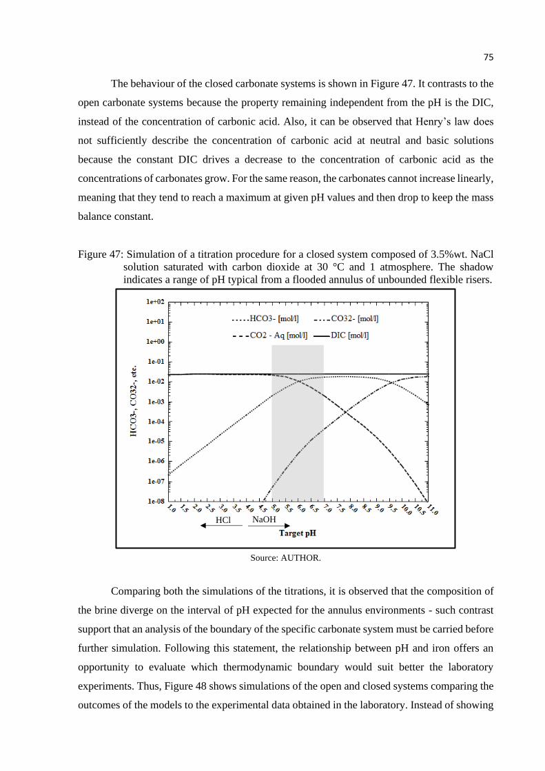
75

The behaviour of the closed carbonate systems is shown in Figure 47. It contrasts to the

open carbonate systems because the property remaining independent from the pH is the DIC,

instead of the concentration of carbonic acid. Also, it can be observed that Henry’s law does

not sufficiently describe the concentration of carbonic acid at neutral and basic solutions

because the constant DIC drives a decrease to the concentration of carbonic acid as the

concentrations of carbonates grow. For the same reason, the carbonates cannot increase linearly,

meaning that they tend to reach a maximum at given pH values and then drop to keep the mass

balance constant.

Figure 47: Simulation of a titration procedure for a closed system composed of 3.5%wt. NaCl

solution saturated with carbon dioxide at 30 °C and 1 atmosphere. The shadow

indicates a range of pH typical from a flooded annulus of unbounded flexible risers.

Source: AUTHOR.

Comparing both the simulations of the titrations, it is observed that the composition of

the brine diverge on the interval of pH expected for the annulus environments - such contrast

support that an analysis of the boundary of the specific carbonate system must be carried before

further simulation. Following this statement, the relationship between pH and iron offers an

opportunity to evaluate which thermodynamic boundary would suit better the laboratory

experiments. Thus, Figure 48 shows simulations of the open and closed systems comparing the

outcomes of the models to the experimental data obtained in the laboratory. Instead of showing

HCl NaOH

76

the data of the low flow rate experiment only, the pH and [Fe2+] data from all laboratory

experiments (N° 1 – low flow rate of CO2; and N° 2 – high flow rate of CO2) is shown. This

was carried with the purpose of increasing the rigorosity and robustness of the analysis.

Figure 48: Comparison between open and closed carbonate systems.

Source: AUTHOR.

The results show that the open carbonate system proves to be a better option for further

simulations, as the simulated pH lies much closer to the experimental ones. Reflecting upon the

underlying assumptions and interactions between the system and neighbourhood, it seems that

open carbonate systems indeed agree better to the process of permeation of carbon dioxide into

the annulus of flexibles and, also, to the experimental setup used in the laboratory, since the

molecules of carbon dioxide may enter and depart the occluded environment.

Following the statement that the open carbonate system could be a better option for

further simulations, a broader view of the effect of the iron on the solution is seen in Figure 49.

The plot comprises the domains of undersaturation, saturation and supersaturation of brines

with iron at 30 °C, and saturated with carbon dioxide in 1 atmosphere. The results show

increasing values of pH, HCO3- and CO3

2- and FeCO3 as the concentration of dissolved iron

increase. The concentration of carbonic acid remained constant and defined by the maximum

solubility of carbon dioxide regarding the pressure and temperature, and so was not shown.

77

Figure 49: Simulation of the composition of the brine as a function of the concentration of Fe2+.

a) pH. b) HCO3-. c) CO3

2-. d) CO2(aq). e) FeCO3. The solution consists of 3.5%wt.

NaCl brine saturated with carbon dioxide at 30 °C and 1 atmosphere.

Source: AUTHOR.

The experimental evolution of the pH was reproduced through simulation based on the

experimental data of [Fe2+]. Figure 50 reveals the good agreement between the experiment and

simulation, presenting minor uncertainties. Nonetheless, it is reasonable to assume that the

nature of the existing the uncertainty lies on the influence of factors such as the modelling

strategies; the accuracy of the databanks; the accuracy range of the pH probe or small

temperature differences that are inherent of the measurement steps.

a) b)

c) d)

78

Figure 50: Simulation and experimental evolution of pH at 3.5% NaCl brine at 30 °C, 1 atm of

CO2 and flow rate of 0.0008 ml.min-1.cm-2.

Source: AUTHOR.

4.3. ELECTROCHEMICAL MONITORING

Open circuit potential (OCP)

The open circuit potentials of the working electrodes were monitored over time. Figure

51 shows the evolution of the OCPs with time. It is seen an initial stage where the OCP of the

working electrodes decreases over the first 500 hrs. Then, the OCP increase in a second stage,

moving towards more noble values. In a third stage, the OCP drop off to a plateau of

approximately -580mV, in the same period over which the pH and iron concentration stabilised,

as shown in the previous sections. In other words, the evolution of OCP can be divided into

three stages: I - an initial reduction over the first hours; II - a dwell at less noble values and a

shift towards more noble values; III – steady state at nobler OCP.

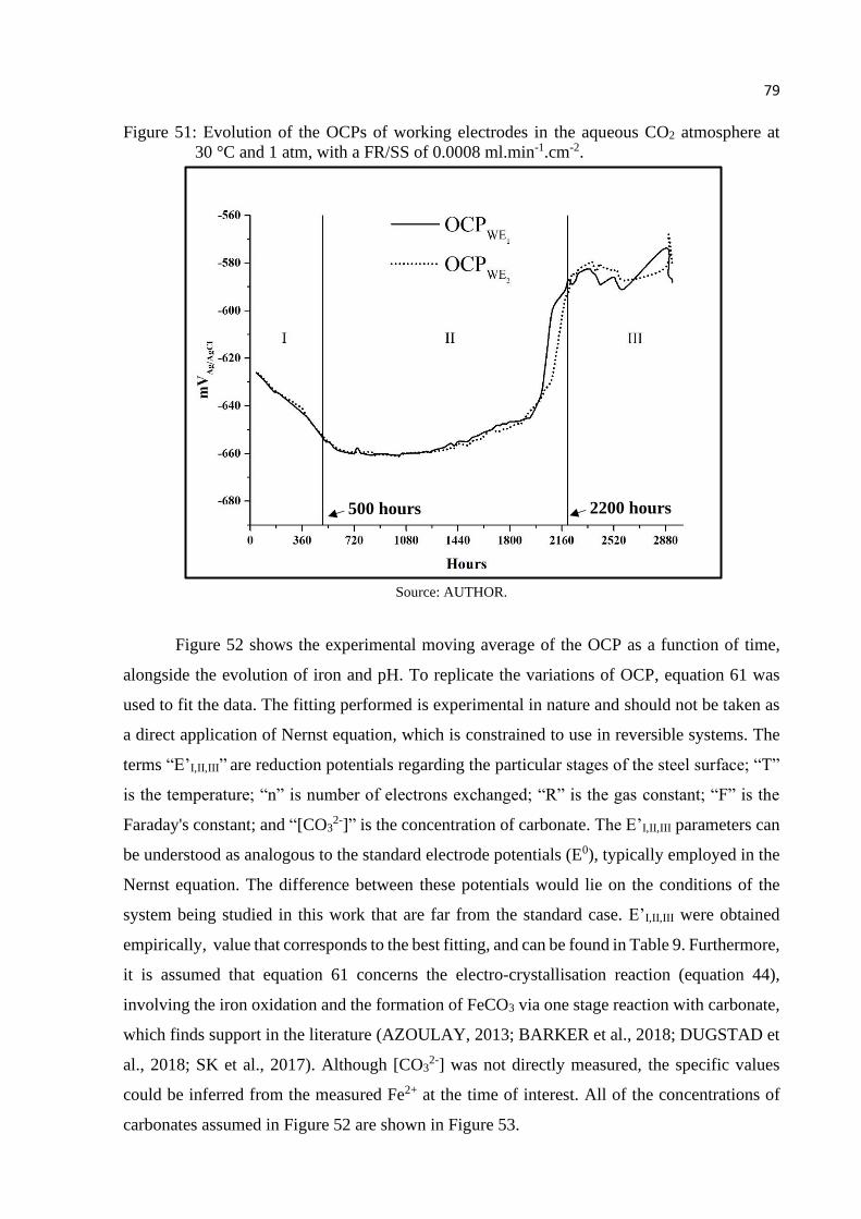
79

Figure 51: Evolution of the OCPs of working electrodes in the aqueous CO2 atmosphere at

30 °C and 1 atm, with a FR/SS of 0.0008 ml.min-1.cm-2.

Source: AUTHOR.

Figure 52 shows the experimental moving average of the OCP as a function of time,

alongside the evolution of iron and pH. To replicate the variations of OCP, equation 61 was

used to fit the data. The fitting performed is experimental in nature and should not be taken as

a direct application of Nernst equation, which is constrained to use in reversible systems. The

terms “E’I,II,III” are reduction potentials regarding the particular stages of the steel surface; “T”

is the temperature; “n” is number of electrons exchanged; “R” is the gas constant; “F” is the

Faraday's constant; and “[CO32-]” is the concentration of carbonate. The E’I,II,III parameters can

be understood as analogous to the standard electrode potentials (E0), typically employed in the

Nernst equation. The difference between these potentials would lie on the conditions of the

system being studied in this work that are far from the standard case. E’I,II,III were obtained

empirically, value that corresponds to the best fitting, and can be found in Table 9. Furthermore,

it is assumed that equation 61 concerns the electro-crystallisation reaction (equation 44),

involving the iron oxidation and the formation of FeCO3 via one stage reaction with carbonate,

which finds support in the literature (AZOULAY, 2013; BARKER et al., 2018; DUGSTAD et

al., 2018; SK et al., 2017). Although [CO32-] was not directly measured, the specific values

could be inferred from the measured Fe2+ at the time of interest. All of the concentrations of

carbonates assumed in Figure 52 are shown in Figure 53.

500 hours 2200 hours

80

E = EI,II,III′ −

2.303RT

nF × log [CO3

2−] (61)

Fe(s) + CO3(aq)−2 ↔ FeCO3(s) + 2e

− (44)

Figure 52: Evolution of the measured and analytical OCP, iron concentration and pH. The plot

shows 3 zones, described by Roman numerals “I”, “II” and “III”. Test conditions:

V/S of 0.2 ml/cm², 3.5%wt. NaCl brine, FR/SS of 0.0008 ml.min-1.cm-2, 1 atm of

CO2 and 30±2 °C.

Source: AUTHOR.

500 hours 2200 hours

81

Figure 53: Simulation of [CO32-] inferred from the measured Fe2+. The modelled electrolyte

consists of 3.5%wt. NaCl brine saturated with carbon dioxide at 30 °C and 1

atmosphere.

Source: AUTHOR.

Table 9: E’I,II,III constants respective to the three stages of OCP.

FR/SS

[ml.min-1.cm-2]

EI’

[VAg/AgCl]

EII’

[VAg/AgCl]

EIII’

[VAg/AgCl]

0.0008 -0.578 -0.607 -0.560

Comparing the experimental moving average OCP with the analytical value, it is

observed that the first is well described by the latter at all stages. This observation supports the

hypothesis that the change in the OCP is a function of iron dissolved in the solution, which in

turn affects the carbonate balance of the system. The transitions of E’ are not easily explained.

However, the variations in pH or the adhesion of FeCO3 in the surface could play important

roles. In other words, the variations in pH may affect E’I,II,III through disturbing the

electrochemical reactions. Thus, at the start, the pH of the solution is more acid so the E’I would

be more positive, as also observed by the effect of pH in usual Evans diagrams. Similarly, as

the pH increases the E’II should become more negative. The coverage of the surface with

protective scales could also affect E’ because the layers of corrosion product may change the

oxidation tendency of the metal, perhaps explaining the later stage behaviour observed.

Moreover, temperature variations could also affect the OCP by changing the slope of equation

61 and by disturbing the solubility of chemical species, including carbonates and carbonic acid.

82

This last relationship was not clear in this work because of the steady temperature control but

may be significant for further testing in larger scales, whose temperatures could fluctuate more.

Linear polarisation resistance (LPR)

The LPR technique provides data of corrosion rate and polarization resistance. It is

known that the corrosion rate data may carry inaccuracies associated with incorrect Stern-Geary

factors (B). Consequently, the ideal discussion would be focused in the data of polarization

resistance, since it is independent of B or corrosion rate. Yet, the literature often supresses the

results of the polarisation resistance, favouring analysis on the corrosion rate. Then, to favour

comparison with the literature, most of the results and discussion within this work, focus on the

corrosion rate data with a clear description of variables used for the calculus of CRLPR.

Figure 54 shows the corrosion rates and the polarisation resistance of the two working

electrodes in the long-term, low flow rate test. The plot demonstrates two corrosion peaks

separated by approximately one month. The variation of the peak corrosion rate for the two

electrodes in the same system likely occurs due to specifics of the surface area of each. Surface

imperfections and differences regarding roughness, residual stresses, or geometry of the surface

are long known factors to cause uncertainties in corrosion tests. The studies of Ko et al. (2015)

and Barker et al. (2018) support this statement. Ko et al. (2015) testified an immediate increase

in current density upon application of an anodic potential in a rough surface mild steel, but an

induction time before the current increased in a sample with a smoother surface. Barker et al.

(2018) stated that the nucleation and growth of FeCO3 crystals in rough surfaces are faster than

in smooth samples. As mentioned in a previous section, the corrosion rates consider a B of 36.7

mV/dec, ba of 0.218 V/dec and a bc of 0.138 V/dec. However, if the ba considered is equal to

the value reported in the literature for the anodic dissolution of iron, that is ~ 28 mV/dec

(KAHYARIAN; BROWN; NEŠIĆ, 2018), the B resultant would be 10.1 mV/dec. Accordingly,

the corrosion rates shown in Figure 54 would decrease about 72% of the value shown in the

plot, although the overall shape of the curve remains independent of the B.

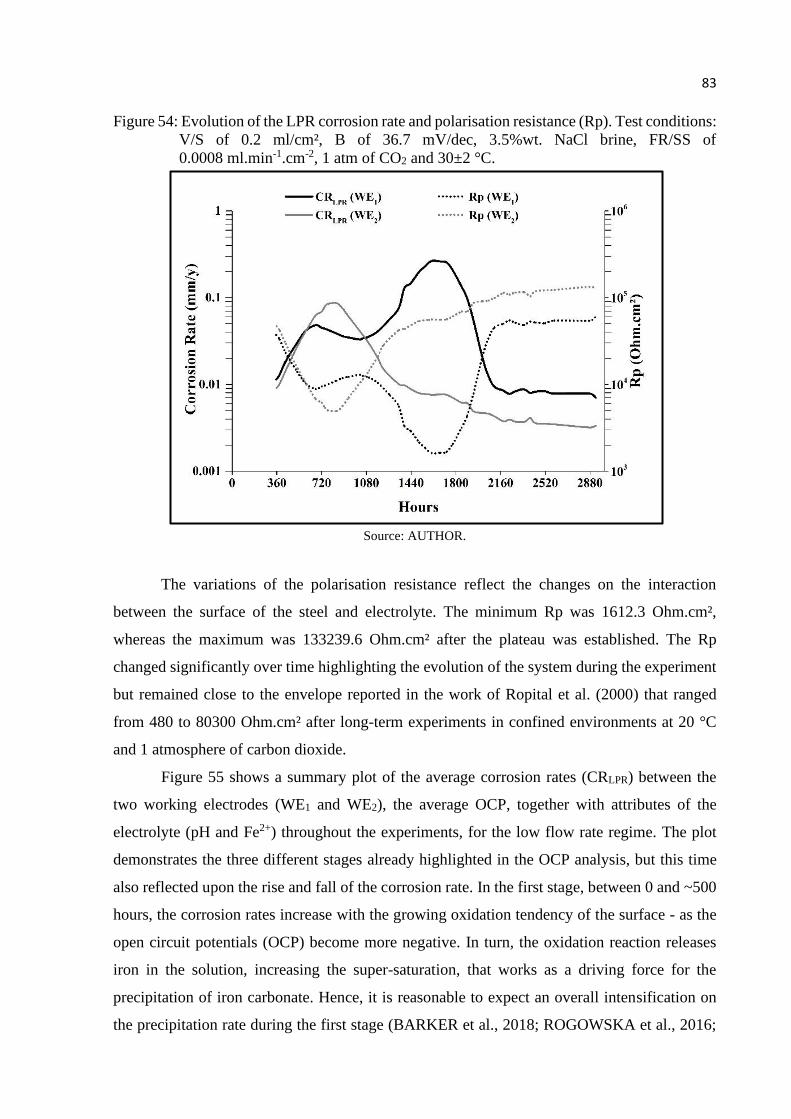
83

Figure 54: Evolution of the LPR corrosion rate and polarisation resistance (Rp). Test conditions:

V/S of 0.2 ml/cm², B of 36.7 mV/dec, 3.5%wt. NaCl brine, FR/SS of

0.0008 ml.min-1.cm-2, 1 atm of CO2 and 30±2 °C.

Source: AUTHOR.

The variations of the polarisation resistance reflect the changes on the interaction

between the surface of the steel and electrolyte. The minimum Rp was 1612.3 Ohm.cm²,

whereas the maximum was 133239.6 Ohm.cm² after the plateau was established. The Rp

changed significantly over time highlighting the evolution of the system during the experiment

but remained close to the envelope reported in the work of Ropital et al. (2000) that ranged

from 480 to 80300 Ohm.cm² after long-term experiments in confined environments at 20 °C

and 1 atmosphere of carbon dioxide.

Figure 55 shows a summary plot of the average corrosion rates (CRLPR) between the

two working electrodes (WE1 and WE2), the average OCP, together with attributes of the

electrolyte (pH and Fe2+) throughout the experiments, for the low flow rate regime. The plot

demonstrates the three different stages already highlighted in the OCP analysis, but this time

also reflected upon the rise and fall of the corrosion rate. In the first stage, between 0 and ~500

hours, the corrosion rates increase with the growing oxidation tendency of the surface - as the

open circuit potentials (OCP) become more negative. In turn, the oxidation reaction releases

iron in the solution, increasing the super-saturation, that works as a driving force for the

precipitation of iron carbonate. Hence, it is reasonable to expect an overall intensification on

the precipitation rate during the first stage (BARKER et al., 2018; ROGOWSKA et al., 2016;

84

SUN, 2006). The second stage is shown in Figure 55 between ~500 and ~2200 hours. It

represents the period of intense generation of iron ions (by corrosion) and intense consumption

of iron ions (by precipitation). During this stage, the corrosion rate, the OCP, the pH and the

composition of the solution are affected by the trade-off between driving forces. Once

precipitation dominates, the concentration of Fe2+ drops and the OCP begins to shift towards

more noble values in line with trends shown in the literature (BARKER et al., 2018; DUGSTAD

et al., 2018; HAN et al., 2007; ROGOWSKA et al., 2016; TANUPABRUNGSUN et al., 2012).

As a result, the corrosion process becomes less favourable, and the corrosion rates decrease

over time. Moreover, the fall of the iron concentration will reduce the level of super-saturation,

and so the associated growth of surface scales. In the third stage, observed after roughly 2200

hours, is characterised by low corrosion rates, stable OCP at the shift towards nobler values,

stable pH and low concentration of iron ions in solution. These characteristics indicate that a

near steady state has been reached.

Figure 55: Evolution of the LPR corrosion rate, OCP, pH and Fe2+. Test conditions: V/S of

0.2 ml/cm², B of 36.7 mV/dec, 3.5%wt. NaCl brine, FR/SS of 0.0008 ml.min-1.cm-2,


Source: AUTHOR.

AVG

85

Comparing the trends in corrosion rates with those reported in the literature, there are

some differences to note. Clements (2008) shows corrosion rates that start at higher values,

during the initial stages of the experiment and decay with time. It is likely that the difference

between behaviours is the result of the different deaeration processes employed. Previous

studies of the annulus corrosion process were carried out in solutions that were deaerated with

carbon dioxide or that contained acid buffers. As a result, it is reasonable to assume that the

concentrations of carbonic acid of these solutions were high from the beginning. Thus, such

experiments begin with relatively aggressive environments and high initial corrosion rates that

decrease over time as iron dissolves into the solution and as a protective scale forms. In the

present case, deaeration was carried out with nitrogen, and the carbonic acid only begins to

form, once the experiment has started, i.e. a less aggressive starting condition, closer to the

reality of a flexible in service.

Linear sweep voltammetry (LSV)

The linear sweep voltammetry (LSV) is used to measure the absolute corrosion rates

and properties of the surface of the steel. Figure 56 and Table 10 show the results of the LSV

analysis. The results show mild corrosion rates and B that agrees with the literature

(ROGOWSKA et al., 2016), though ba seems larger than could be expected in case of active

dissolution of iron in CO2 containing environments. Kahyarian; Brown; Nešić (2018)

performed corrosion tests in API X65 steel in CO2-containing solution at 30 °C and observed

that the ba from the stage of active dissolution should range between 0.030 to 0.040 V/dec in

respect to the pH. However, the stage before passivation, named pre-passivation, the apparent

slope is around 0.120 V/dec. Therefore, the relatively large ba point toward the build-up of a

protective scale. From the works of Hernandez; Muñoz; Genesca, (2012) and Kahyarian;

Brown; Nešić, (2018) it is possible to expect that the cathodic branch would show a mass-

controlled mechanism. Despite that, the mass-controlled behaviour is not clear, and further

work should be carried to understand such phenomenon. Nevertheless, Hernandez; Muñoz;

Genesca, (2012) conducted LSV using a rotating electrode setup, observed bc ranging from

0.120 to 0.153 V/dec, meaning that the data obtained in this work is consistent to the literature.

86

Figure 56: Plot of the linear sweep voltammetry at test end. Test conditions: 1 mV/s, V/S of


30±2 °C.

Source: AUTHOR.

Table 10: Results of the linear sweep voltammetry at test end. Test conditions: V/S of

0.2 ml/cm², 3.5%wt. NaCl brine, FR/SS of 0.0008 ml.min-1.cm-2, 1 atm of CO2 and 30±2 °C.

FR/SS Ecorr jcorr CRLSV ba bc B Time

[ml/min/cm2] [VAg/AgCl] [A/cm²] [mm/y] [V/dec] [V/dec] [mV/dec] [months]

0.0008 -0.673 5.4E-08 0.0006 0.218 0.138 36.7 4

Figure 57 was adapted from the study of Remita et al. (2008), relevant to annulus

environments. The plot compares the experimental CRLSV to their predictions of the annulus.

The model is of interest because it introduces the variable θ, which is related to the coverage of

the surface by a protective scale (e.g. FeCO3) or grease. According to the authors, a fully

covered surface (θ = 1) implies that the thermodynamic equilibrium has been reached. When θ

is equal to 0, the surface of the steel is active. Interestingly, their model seems to fit very well

the CRLSV when θ is equal to 0.99, which agrees to the growth of a protective scale and the

achievement of the steady state that was mentioned in the previous sections.

87

Figure 57: Comparison of the corrosion rates obtained by LSV to results described in the

literature at different degrees of occlusion.

Source: AUTHOR and data extracted from (REMITA et al., 2008).

4.4. WEIGHT CHANGE TECHNIQUES

Average corrosion rates and average scale growth

Weight change methods provide average values of corrosion rate and scale growth

respective to the total duration of the experiments. The average corrosion rate (ACR) was

calculated using equation 55, and the average scale growth (ASG) using equation 57. For the

tolerance interval, it is assumed that 90% of the population have the ACR or ASG falling within

the bounds of the tolerance interval with 95% confidence. The tolerance interval was calculated

using the normal tolerance method, as the data distribution was normal. Outliers were detected

and excluded from the weight change analysis. The abnormal values were attributed to practical

issues or the sharing of corrosion products from neighbour samples. The results of the weight

change analyses are shown in Table 11, presenting the mean values, the tolerances, the data

distribution and the number of identification of the respective samples considered as outliers.

REMITA et al., 2008

88

ACR =m1−m3

MWFe×t×S×365×24×MWFe

ρ (55)

ASG =m2−m3

MWFeCO3×t×S (57)

Table 11: Average corrosion rate (ACR) and average scale growth (ASG) of high strength

steel tensile wires in 3.5%wt. NaCl, at 1 atm of CO2 and 30±2 °C.

Test ACR [mm/y] Distribution Outliers

[Id. N°]

ASG

[mol/(m²h)]

Outliers

[Id. N°] Distribution

FR/SS=0.0008

ml.min-1.cm-2

(4 Months,

0.2 ml/cm²)

0.0177 0.00230.0331 Normal

04, 08,

14 2.67E−041.83𝐸−043.51𝐸−04

02, 04,

08 Normal

The ACR observed was 0.0177 mm/y (2.84E-04 mol/(m²h)). Thought this value is

relatively small, it is almost an order of magnitude larger than the value provided by the linear

voltammetry analysis. The reason behind such a difference is that the ACR is an average value,

whereas CRLSV is an absolute value respective to the end of the test, meaning that the values

are not comparable.

Moreover, although it is common to find the use of gravimetric measures in the literature

(CLEMENTS, 2008; CLEMENTS; ETHRIDGE, 2003; DUGSTAD et al., 2018; RUBIN et al.,

2012; UNDERWOOD, 2002), its use should be restricted to applications where the corrosion

rate does not change considerably in time, since the average values does not describe the trends

nor absolute values. Therefore, a better use of the ACR and ASG results is a determination of

the scaling tendency (ST). The ST is a non-dimentional parameter based on the ratio between

the ASG and the ACR in the same unit. It characterises the kinetics and the protectiveness of

corrosion scales formed on the surface of the steel. In the long term low flow rate experiment

the ST obtained was 0.938, which is close to the unity, meaning that the scale growth remained

as important as the corrosion process. Note that if the overall trend of the critical ST shown in

Figure 43 is kept, it can be assumed that the ST above 93% would be relatively higher than the

critical value. Thus, the scale adhered in the surface is understood as protective. Besides that,

the establishment of a steady state with low corrosion rates, as shown in the previous sections,

also agrees with such an interpretation.

To observe the results in a wider context with relevant literature in the field, Figure 58

shows the results of ACR and CRLSV alongside others digitally extracted from works published

in similar conditions (filtered to temperature ranges from 20 to 30 °C in atmospheric pressures

89

consisting of pure CO2). The literature data involves several test durations and different

techniques to obtain corrosion rate, including weight loss, LPR and LSV. The plot reveals that

the range of results obtained in this work has some overlap with the literature data (DUGSTAD

et al., 2015; ROPITAL et al., 2000; RUBIN et al., 2012; SUN, 2006). Also, despite the

significant differences in the occlusion ratios, the corrosion rates found in the work of Dugstad

et al. (2015) were close regarding magnitudes. This similarity is explained by the high degrees

of supersaturation with iron, similar to occluded systems, that was artificially induced by the

authors. Such a comparison shed light on the importance of iron concentration on the study of

the annulus environment.

Figure 58: Comparison of the corrosion rates to results described in the literature at different

degrees of occlusion.

Source: AUTHOR and data extracted from (DUGSTAD et al., 2015; ROPITAL et al., 2000; RUBIN et al., 2012;

SUN, 2006).

[DUGSTAD et al., 2015]

[DUGSTAD et al., 2015]

[SUN, 2006]

[RUBIN et al., 2012]

[ROPITAL et al., 2000]

[RUBIN et al., 2012]

[ROPITAL et al., 2000]

90

4.5. CORROSION SURFACE EXAMINATION

Figure 59 shows the most repeated surface appearances before and after the test. In

many samples a uniform layer of scale was evident. Besides, no pitting or localised differences

in corrosion that could not be linked to imperfections in the starting surface condition were

identified. The experiment also produced a number of surfaces that displayed disruptions in the

corrosion scales in the shape of bubbles, highlighted by the black arrows. It is understood that

bubbles may form on the surface as a consequence of the hydrogen reduction reaction, or due

to the high degree of occlusion that can induce mechanical trapping of CO2 bubbles between

neighbour samples.

Figure 59: Representative corrosion surface of the samples, demonstrating the specimens before

and after the test. Test conditions: V/S of 0.2 ml/cm², 3.5%wt. NaCl brine, FR/SS of


Source: AUTHOR.

The surfaces of the WE sample, whose potential was not swept by an LSV test, was

observed before and after the four months in the solution (see Figure 60). The images taken by

a light microscope immediately after the test vessel was opened show darkening of the surface

with no apparent signs of localised corrosion. After a brief period in the open atmosphere, the

dark corrosion products turned yellow.

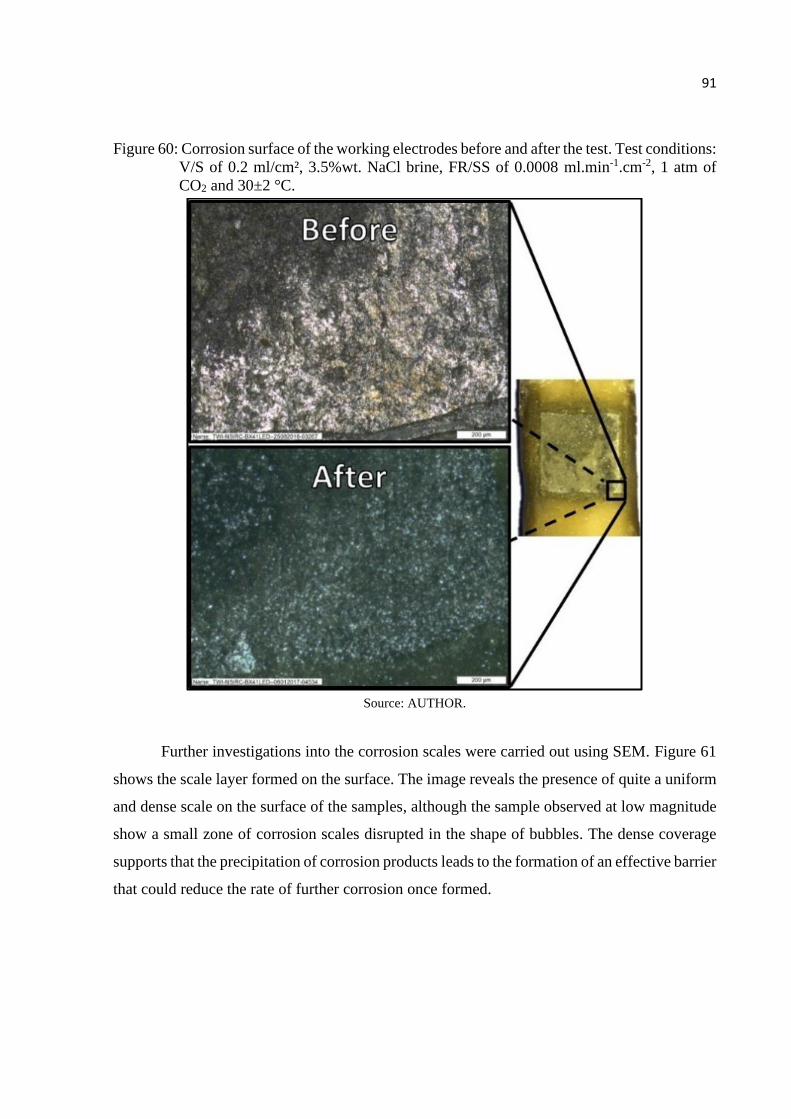
91

Figure 60: Corrosion surface of the working electrodes before and after the test. Test conditions:

V/S of 0.2 ml/cm², 3.5%wt. NaCl brine, FR/SS of 0.0008 ml.min-1.cm-2, 1 atm of

CO2 and 30±2 °C.

Source: AUTHOR.

Further investigations into the corrosion scales were carried out using SEM. Figure 61

shows the scale layer formed on the surface. The image reveals the presence of quite a uniform

and dense scale on the surface of the samples, although the sample observed at low magnitude

show a small zone of corrosion scales disrupted in the shape of bubbles. The dense coverage

supports that the precipitation of corrosion products leads to the formation of an effective barrier

that could reduce the rate of further corrosion once formed.

92

Figure 61: SEM images of corrosion scale formed after four months of testing. Top and bottom

surfaces of the selected tensile wire are shown. Test conditions: 3.5%wt. NaCl, 1 atm

of CO2, FR/SS of 0.0008 ml.min-1.cm-2 and 30±2 °C.

Source: AUTHOR.

A definitive characterisation of the corrosion scale is obtained by XRD analysis, shown

in Figure 62, which demonstrates large peaks of FeCO3. Note that such information also

supports the usage of the term MWFeCO3 in equation 57, used to determine the average scale

growth.

Bo

tto

m s

urf

ace

To

p s

urf

ace

93

ASG =m2−m3

MWFeCO3×t×S (57)

Figure 62: XRD results confirming the presence of FeCO3 on the surface of a sample after the

test. Test conditions: 3.5%wt. NaCl, 1 atm of CO2, FR/SS of 0.0008 ml.min-1cm-2

and 30±2 °C.

Source: AUTHOR.

4.6. EFFECT OF THE FLOW RATE OF CO2

Studies exploring the effect of flow rate on the risk of sulphide stress cracking in H2S-

containing environments identified that the restriction of flow rate could influence the steady

state concentration of this aggressive species in the simulated annular conditions (DÉSAMAIS;

TARAVEL-CONDAT, 2009; HAAHR et al., 2016). These assertions suggest that a restricted

flux of CO2 into a system may alter the steady state conditions and time that it takes for it to be

established. This, in turn, may affect the corrosion rate of steel within it. Based on these

considerations, an additional experiment was carried with a controlled high flow rate (two

orders of magnitude larger) for two months, in order to study the influence of CO2 flow rate on

the corrosion of steel in annular environments. It is important to highlight that the high flow

rate short-term experiment followed the same methodology and analyses as the others done in

the low flow long-term experiment. The differences and similarities were explored regarding

the evolution of iron and pH, the simulation characteristics, the electrochemical properties, the

corrosion rates, the scale growth and the corrosion surface.

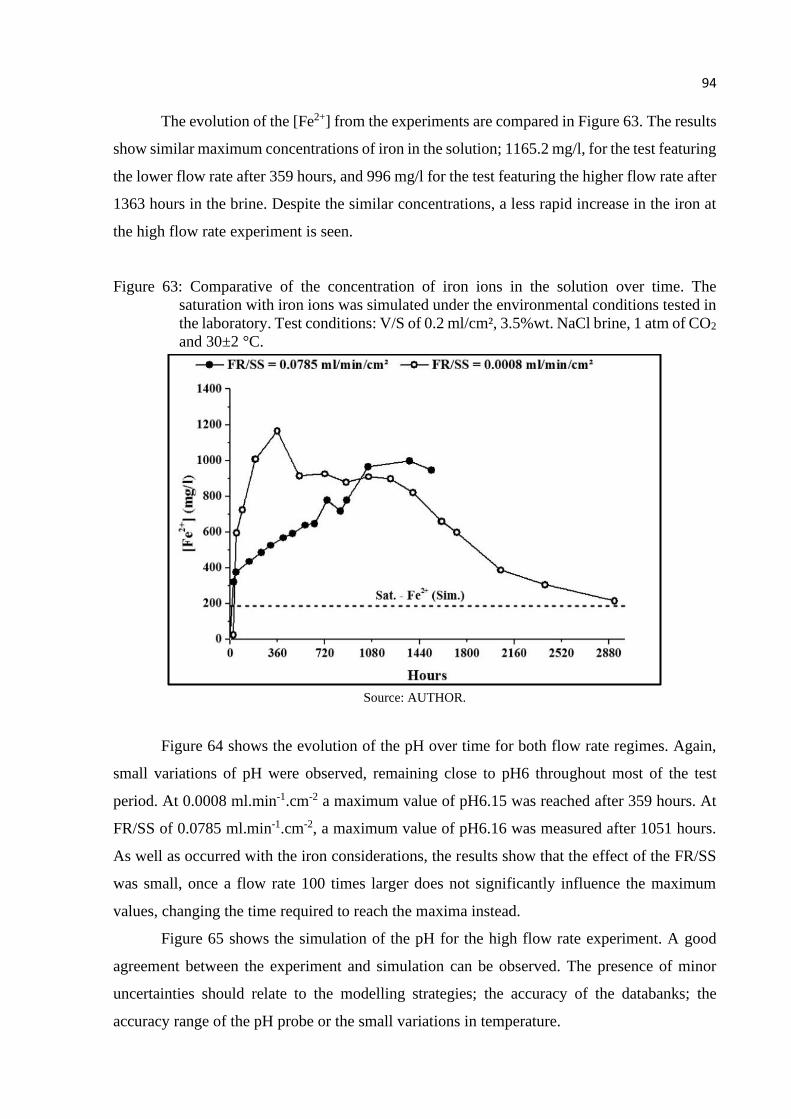
94

The evolution of the [Fe2+] from the experiments are compared in Figure 63. The results

show similar maximum concentrations of iron in the solution; 1165.2 mg/l, for the test featuring

the lower flow rate after 359 hours, and 996 mg/l for the test featuring the higher flow rate after

1363 hours in the brine. Despite the similar concentrations, a less rapid increase in the iron at

the high flow rate experiment is seen.

Figure 63: Comparative of the concentration of iron ions in the solution over time. The

saturation with iron ions was simulated under the environmental conditions tested in

the laboratory. Test conditions: V/S of 0.2 ml/cm², 3.5%wt. NaCl brine, 1 atm of CO2

and 30±2 °C.

Source: AUTHOR.

Figure 64 shows the evolution of the pH over time for both flow rate regimes. Again,

small variations of pH were observed, remaining close to pH6 throughout most of the test

period. At 0.0008 ml.min-1.cm-2 a maximum value of pH6.15 was reached after 359 hours. At

FR/SS of 0.0785 ml.min-1.cm-2, a maximum value of pH6.16 was measured after 1051 hours.

As well as occurred with the iron considerations, the results show that the effect of the FR/SS

was small, once a flow rate 100 times larger does not significantly influence the maximum

values, changing the time required to reach the maxima instead.

Figure 65 shows the simulation of the pH for the high flow rate experiment. A good

agreement between the experiment and simulation can be observed. The presence of minor

uncertainties should relate to the modelling strategies; the accuracy of the databanks; the

accuracy range of the pH probe or the small variations in temperature.

95

Figure 64: pH values as a function of time and FR/SS of CO2. Test conditions: V/S of

0.2 ml/cm², 3.5%wt. NaCl brine, at 1 atm of CO2 and 30±2 °C.

Source: AUTHOR.

Figure 65: Simulation and experimental evolution of pH at 3.5% NaCl brine at 30 °C, 1 atm of

CO2 and flow rate of 0.0785 ml.min-1.cm-2.

Source: AUTHOR.

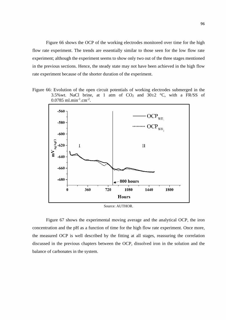
96

Figure 66 shows the OCP of the working electrodes monitored over time for the high

flow rate experiment. The trends are essentially similar to those seen for the low flow rate

experiment; although the experiment seems to show only two out of the three stages mentioned

in the previous sections. Hence, the steady state may not have been achieved in the high flow

rate experiment because of the shorter duration of the experiment.

Figure 66: Evolution of the open circuit potentials of working electrodes submerged in the

3.5%wt. NaCl brine, at 1 atm of CO2 and 30±2 °C, with a FR/SS of

0.0785 ml.min-1.cm-2.

Source: AUTHOR.

Figure 67 shows the experimental moving average and the analytical OCP, the iron

concentration and the pH as a function of time for the high flow rate experiment. Once more,

the measured OCP is well described by the fitting at all stages, reassuring the correlation

discussed in the previous chapters between the OCP, dissolved iron in the solution and the

balance of carbonates in the system.

800 hours

97

Figure 67: Evolution of the average open circuit potentials, fitting OCP curves, iron in solution

and pH. The plot shows two stages, described by Roman numerals “I” and “II”. Test



Source: AUTHOR.

Figure 68 shows the evolution of the Rp and CRLPR for the high flow rate experiment.

Though a considerable Rp (107468.8 Ohm.cm²) was seen at the beginning of the test, the

maximum Rp has not been established within the test timeframe due to the shorter duration of

the experiment. The minimum Rp observed was 1661.6 Ohm.cm² at the peak CRLPR, which is

very close to the minimum value seen for the low flow rate experiment (1612.3 Ohm.cm²).

The Rp analysis allows a direct comparison between the two flow rate conditions since

it is independent of B. Therefore, Figure 69 shows the evolution of Rp with time for the two

flow rates investigated that achieved the respective lowest Rp. Apart from the time needed to

reach the minimum Rp, no substantial difference between them is seen.

800 hours

98

Figure 68: Evolution of the LPR corrosion rate and polarisation resistance (Rp). Test conditions:

V/S of 0.2 ml/cm², B of 36.7 mV/dec, 3.5%wt. NaCl brine, FR/SS of


Source: AUTHOR.

Figure 69: Comparison of Rp of working electrodes with respect to the flow rates employed in

the experiments. Test conditions V/S of 0.2 ml/cm², 3.5%wt. NaCl brine, 1 atm of

CO2 and 30±2 °C.

Source: AUTHOR.

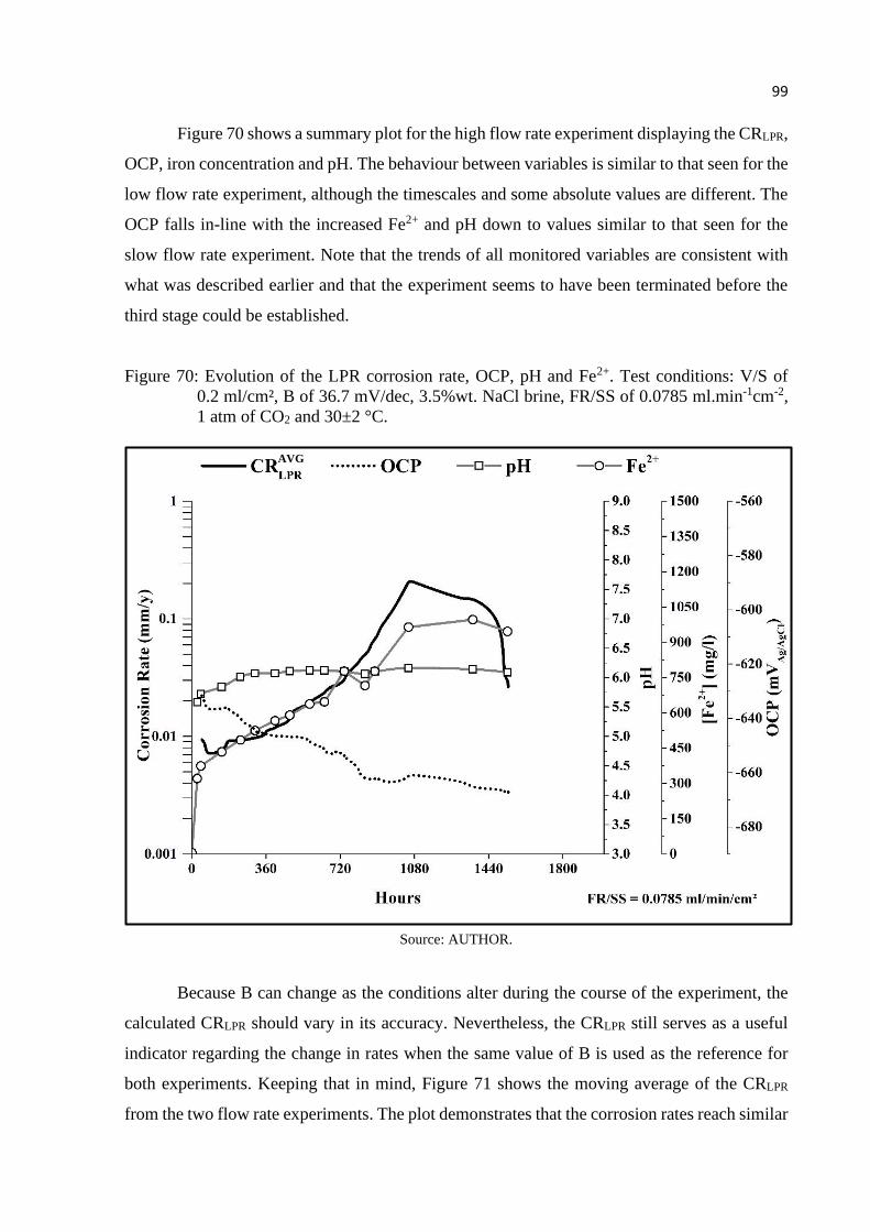
99

Figure 70 shows a summary plot for the high flow rate experiment displaying the CRLPR,

OCP, iron concentration and pH. The behaviour between variables is similar to that seen for the

low flow rate experiment, although the timescales and some absolute values are different. The

OCP falls in-line with the increased Fe2+ and pH down to values similar to that seen for the

slow flow rate experiment. Note that the trends of all monitored variables are consistent with

what was described earlier and that the experiment seems to have been terminated before the

third stage could be established.

Figure 70: Evolution of the LPR corrosion rate, OCP, pH and Fe2+. Test conditions: V/S of

0.2 ml/cm², B of 36.7 mV/dec, 3.5%wt. NaCl brine, FR/SS of 0.0785 ml.min-1cm-2,


Source: AUTHOR.

Because B can change as the conditions alter during the course of the experiment, the

calculated CRLPR should vary in its accuracy. Nevertheless, the CRLPR still serves as a useful

indicator regarding the change in rates when the same value of B is used as the reference for

both experiments. Keeping that in mind, Figure 71 shows the moving average of the CRLPR

from the two flow rate experiments. The plot demonstrates that the corrosion rates reach similar

AVG

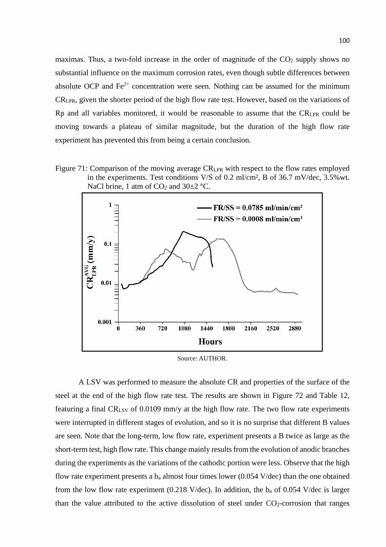
100

maximas. Thus, a two-fold increase in the order of magnitude of the CO2 supply shows no

substantial influence on the maximum corrosion rates, even though subtle differences between

absolute OCP and Fe2+ concentration were seen. Nothing can be assumed for the minimum

CRLPR, given the shorter period of the high flow rate test. However, based on the variations of

Rp and all variables monitored, it would be reasonable to assume that the CRLPR could be

moving towards a plateau of similar magnitude, but the duration of the high flow rate

experiment has prevented this from being a certain conclusion.

Figure 71: Comparison of the moving average CRLPR with respect to the flow rates employed

in the experiments. Test conditions V/S of 0.2 ml/cm², B of 36.7 mV/dec, 3.5%wt.

NaCl brine, 1 atm of CO2 and 30±2 °C.

Source: AUTHOR.

A LSV was performed to measure the absolute CR and properties of the surface of the

steel at the end of the high flow rate test. The results are shown in Figure 72 and Table 12,

featuring a final CRLSV of 0.0109 mm/y at the high flow rate. The two flow rate experiments

were interrupted in different stages of evolution, and so it is no surprise that different B values

are seen. Note that the long-term, low flow rate, experiment presents a B twice as large as the

short-term test, high flow rate. This change mainly results from the evolution of anodic branches

during the experiments as the variations of the cathodic portion were less. Observe that the high

flow rate experiment presents a ba almost four times lower (0.054 V/dec) than the one obtained

from the low flow rate experiment (0.218 V/dec). In addition, the ba of 0.054 V/dec is larger

than the value attributed to the active dissolution of steel under CO2-corrosion that ranges

AV

G

101

between 0.022 to 0.040 V/dec, but almost half of the value attributed in literature for the

mechanism of pre-passivation of steel (0.120 V/dec) (BARKER et al., 2018; KAHYARIAN;

BROWN; NEŠIĆ, 2018). Therefore, considering the ba reported by the literature, it could be

presumed an incomplete coverage of scale in the surface of the samples in the high flow rate

experiment, providing partial protection for the steel. Concerning the cathodic branch, the

experiment with a higher flow rate exhibited a larger bc that could be expected from the values

observed in low flow rate experiment and literature (HERNANDEZ; MUÑOZ; GENESCA,

2012). To understand this result, more experiments would be required. Anyhow, the

establishment of mixed mechanisms (charge and mass controlled) is a hypothesis that cannot

be discarded.

Figure 72: Linear sweep voltammetry at test end. Test conditions: V/S of 0.2 ml/cm², 3.5%wt.


Source: AUTHOR.

Table 12: Linear sweep voltammetry at test end. Test conditions: V/S of 0.2 ml/cm², 3.5%wt.


FR/SS Ecorr jcorr CR ba bc B Time

[ml/min/cm2] [VAg/AgCl] [A/cm²] [mm/y] [V/dec] [V/dec] [mV/dec] [months]

0.0785 -0.694 9.4E-07 0.0109 0.054 0.211 18.6 2

0.0008 -0.673 5.4E-08 0.0006 0.218 0.138 36.7 4

102

Figure 73 compares the CRLSV of the high flow rate experiment with the model proposed

by Remita et al. (2008). It is observed that the corrosion rates in the high flow rate experiment

fit a θ close to 0.5, instead of the value close to 0.99 observed in the low flow rate experiment.

These results not only support that the coverage of the scale and the protection it offers is only

partial in the high flow experiment, but also that the corrosion process has not reached a steady

state after two months.

Figure 73: Comparison of the corrosion rates obtained by LSV to results described in the

literature at various degrees of occlusion.

Source: AUTHOR with data extracted from (REMITA et al., 2008).

Table 13 shows the results of the weight change analyses. A nonparametric method was

used to calculate the tolerances interval respective to the high flow rate experiment since the

data distribution was non-normal. The attempts to transform the data to obtain a normal

distribution were not successful. An ACR of 0.0211 mm/y (3.41E-04 mol/(m²h)) was obtained

at the high flow rate. The apparent increase in ACR is likely due to the less extended duration

of the test, which prevented the drop off in rate associated with precipitation and establishment

of a steady state. As well as observed in the low flow rate experiment, the high flow rate

experiment showed a considerable ASG in comparison to ACR. The ST obtained was 0.978,

which is close to one; meaning that the scale covering the surface of the steel seems to be

protective (see Table 14).

REMITA et al., 2008

103

Table 13: Average corrosion rate (ACR) and average scale growth (ASG) of high strength

steel tensile wires corroded in 1 atm of CO2 and 30±2 °C.

Test ACR [mm/y] Distribution Outliers

[Id. N°] ASG [mol/(m²h)]

Outliers

[Id. N°] Distribution

FR/SS=0.0785

ml.min-1cm-2

(2 Months, 0.2

ml/cm²)

0.02110.00300.0653

Non-

normal

15,17,

28 3.34E−042.03𝐸−04

4.86𝐸−04 17,36

Non-

normal

FR/SS=0.0008

ml.min-1cm-2

(4 Months, 0.2

ml/cm²)

0.0177 0.00230.0331 Normal

04, 08,

14 2.67E−041.83𝐸−043.51𝐸−04

02, 04,

08 Normal

Table 14: Scaling tendencies of the laboratory experiments.

FR/SS [ml.min-1cm-2] ACR [mol/(m²h)] ASG [mol/(m²h)] ST

0.0785 3.41E-04 3.34E-04 0.978

0.0008 2.84E-04 2.67E-04 0.938

Figure 74 show the corrosion surfaces of the high flow rate experiment viewed in low

magnification, and Figure 75 viewed by light microscopy. The images show that the different

environmental conditions studied produced similar corrosion products, i.e. darkening of the

surface, with no pitting or localised corrosion. Scales uniformly distributed in the samples and

disturbed by bubbles (black arrows) were also frequent for all laboratory experiments.

104

Figure 74: Representative corrosion surface of the samples, demonstrating the specimens before

and after the test. Test conditions: V/S of 0.2 ml/cm², 3.5%wt. NaCl brine, FR/SS of

0.0785 ml.min-1cm-2, 1 atm of CO2 and 30±2 °C.

Source: AUTHOR.

105

Figure 75: Comparison of the corrosion surface of the working electrodes before and after the

test. Test conditions: V/S of 0.2 ml/cm², 3.5%wt. NaCl brine, FR/SS of

0.0785 ml.min-1cm-2, 1 atm of CO2 and 30±2 °C.

Source: AUTHOR.

Figure 76 shows the SEM image of corrosion scale formed during the high flow test

over the shorter term of two months, which appeared to have less continuous scale coverage

than seen for the low flow rate experiment. It is possible that the heterogeneous nature of the

coverage could be resultant of the proximity or contact between adjacent specimens. Five zones

were identified (A-E) as per the annotations. Zone A, shown in Figure 77, is a bare metal

surface. Zone B shown in Figure 78, shows clusters of corrosion products that can also be seen

in the literature (LIU et al., 2016, 2017). Zone C, shown in Figure 79, reveals fine corrosion

products. Zone D, shown in Figure 80, features coarser corrosion particles. Perhaps, the

presence of distinct grain sizes could be explained by the current stage in the iron carbonate

crystallisation process, such as nucleation or crystal growth (BARKER et al., 2018; SUN;

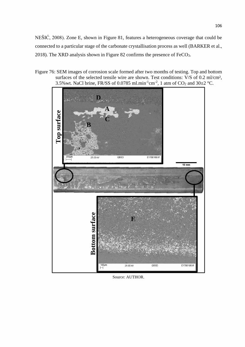
106

NEŠIĆ, 2008). Zone E, shown in Figure 81, features a heterogeneous coverage that could be

connected to a particular stage of the carbonate crystallisation process as well (BARKER et al.,

2018). The XRD analysis shown in Figure 82 confirms the presence of FeCO3.

Figure 76: SEM images of corrosion scale formed after two months of testing. Top and bottom

surfaces of the selected tensile wire are shown. Test conditions: V/S of 0.2 ml/cm²,

3.5%wt. NaCl brine, FR/SS of 0.0785 ml.min-1cm-2, 1 atm of CO2 and 30±2 °C.

Source: AUTHOR.

B

D

\\\\\\\\\

\\\\\\\\\

\\\\\\\\\

\\\\\\\\\

\\\

C

A

To

p s

urf

ace

Bo

tto

m s

urf

ace

E

107

Figure 77: Detail of zone A in Figure 76. Test conditions: V/S of 0.2 ml/cm², 3.5%wt. NaCl

brine, FR/SS of 0.0785 ml.min-1cm-2, 1 atm of CO2 and 30±2 °C.

Source: AUTHOR.

Figure 78: Detail of zone B in Figure 76. Test conditions: V/S of 0.2 ml/cm², 3.5%wt. NaCl

brine, FR/SS of 0.0785 ml.min-1.cm-2, 1 atm of CO2 and 30±2 °C.

Source: AUTHOR.

108

Figure 79: Detail of zone C in Figure 76. Test conditions: V/S of 0.2 ml/cm², 3.5%wt. NaCl


Source: AUTHOR.

Figure 80: Detail of zone D in Figure 76. Test conditions: V/S of 0.2 ml/cm², 3.5%wt. NaCl


Source: AUTHOR.

109

Figure 81: Detail of zone E in Figure 76. Test conditions: V/S of 0.2 ml/cm², 3.5%wt. NaCl


Source: AUTHOR.

Figure 82: XRD results confirming the presence of FeCO3 on the surface of a sample after the

test. Test conditions: 3.5%wt. NaCl, 1 atm of CO2, FR/SS of 0.0785 ml.min-1.cm-2

and 30±2 °C.

Source: AUTHOR.

110

Overall, the absence of considerable differences in the corrosion process after a two-

fold increase in the flow rates seems, at first glance, to contradict the information reported by

Haahr et al. (2016) and Désamais; Taravel-Condat (2009), where new steady state conditions

were found. The authors assumed that the consumption of H2S via corrosion is massive in

comparison to the supply in sour service flexible pipes. Consequently, the remaining

constituents of the gas (CO2) would dominate the steady state of the system, i.e. a less

aggressive steady state. However, this work realises that the same logic does not apply to pure

CO2-corrosion. It is believed that the specifics of the homogeneous chemical reactions of the

H2O/CO2 system on the rate of electrochemical reactions are the cause of such difference. Note

that carbon dioxide undergoes slight hydration to H2CO3 - only ~ 0.26 % (KAHYARIAN;

BROWN; NEŠIĆ, 2018) - meaning that even when the flow rate was low, there was plenty

reactant available to replenish the consumed H2CO3. Moreover, one may notice that basic

theory also supports the results from tests carried in this work once FR/SS is a kinetic variable,

and so, by definition, it shall not affect the thermodynamics of the system (AMERICAN

SOCIETY FOR METALS INTERNATIONAL, 2003). In other words, the difference between

the present case and the works of Haahr et al. (2016) and Désamais; Taravel-Condat (2009) lies

in the types of gas employed and their interactions with the water and the electrochemical

reactions.

4.7. FURTHER CHALLENGES, OPPORTUNITIES AND RESEARCH AREAS FOR

EXPLORING THE ANNULUS CO2-CORROSION OF HIGH STRENGTH STEEL

Based on all that has been observed from the laboratory experiments, from observing

the correlations between multiple variables, from simulations, and also from the fact that the

CO2-corrosion essentially relies on the electrochemical interaction between the electrolyte and

the surface of the steel; this topic explores the effect of the atmospheric variables by expanding

the simulation towards various pressures, temperatures, and concentrations of dissolved iron in

the solution. Plausible states of the electrolyte are investigated in search for more critical

corrosion patterns. However, it is not intended to provide an assessment or a holistic view of

the corrosion process; instead, it is intended to feed the discussion with more data. This chapter

recognise the possibility of the potential existence of unknown variables required to represent

the harsher environmental conditions in the annulus. However, it was impractical to study a

bigger number of variables in the current stage, as additional field information or laborious

laboratory investigations would be required.

111

Effects of atmospheric variables on CO2-containing brines

A screening of pressure and temperature was performed to explore the hydrochemistry

of the brine in the absence of iron ions. The focus is on defining the most aggressive electrolytes

when the iron concentration can be neglected. That is, to the initial stages of corrosion or at

unrepaired failures of the outer sheath revealing a portion of tensile armour directly to the

seawater, currents and tides.

This work assumes that the combination of lower temperatures and higher hydrostatic

pressures resemble the case of breaches of the outer sheath at greater depths, whereas high

temperatures combined with low pressures could characterise unrepaired failures near the

surface; because, the temperature of seawater decreases with depth and pressure increase by 1

atmosphere with every 10 metres of depth. Bearing that in mind, Figure 83 shows the pH of the

NaCl 3.5%wt. brine at pressures and temperatures below and above the critical point of CO2

(31.1 °C and 72.9 atm). The results reveal acidification of the brine as the pressure increase,

which is explained by the fact that pressure raises the solubility limit of H2CO3, favouring the

release of hydrogen ions in the solution, after the chemical dissociation reactions.

Consequently, the steeper slopes of acidification at pressures below 7~10 atmospheres would

suggest a substantial increase of corrosion rates, but also indicate that the effect of pressure in

the corrosion rates could be smaller beyond the range of 1-10 atm. The work of Choi and Nešić

(2011) seems to be in line with this assumption, as the authors performed CO2-corrosion tests

in a pressure range between 40 to 80 bar (39.5 to 79 atm) that resulted on high corrosion rates

but no considerable increase with pressure at the range evaluated.

112

Figure 83: Effect of pressure and temperature on the pH of 3.5%wt. NaCl solution saturated

with carbon dioxide.

Source: AUTHOR.

It is known that substantial variations on the corrosion rates can occur when the

temperatures of the flooded sections of the pipe change, due to variations in the kinetics of the

system. In general, the increase of temperature increases the corrosion rates. However, in the

range evaluated, the statement above contrasts with the thermodynamic point of view presented

by Figure 84, because it shows that the increase of temperature decrease the solubility of carbon

dioxide, which shall result in less aggressive solutions. Therefore, to understand the effect of

the variables and to select the variables of further testing of the annulus, it is imperative to bear

in mind the consequences in the field of kinetics and thermodynamics.

113

Figure 84: Solubility limit of carbon dioxide and pH in 3.5%wt. NaCl brine as a function of

temperature and pressure. a) 5 °C. b) 30 °C. c) 60 °C. d) 90 °C. e) Comparative.

Source: AUTHOR.

Furthermore, the curves beneath the critical temperature of the carbon dioxide (31.1 °C)

present a discontinuity coinciding to the point where the carbon dioxide change from gas to a

liquid phase. This way, the concentration of carbon dioxide and the pH stabilise after the

transition. Such a behaviour can be beneficial for further experimental testing of the annulus

CO2-since it shows that it may not be advantageous to increase the pressure much beyond the

phase transition at temperatures below the critical point because [CO2(aq)] would not change

e)

a) b)

c) d)

114

that much. The fact that safety and practical test requirements usually escalate with the working

pressure of the test vessel would justify this approach. Above the supercritical temperatures and

pressures, the fluid cannot be clearly distinguished between gas and liquid. This is portrayed by

the smoother curves of CO2 solubilities and pH.

Another opportunity to simplify further corrosion testing involves the typical

procedures of pre-saturation or re-saturation with CO2 for tests at higher pressures and warm

temperatures. These procedures generally involve bubbling of gas in an auxiliary vessel to

achieve the saturation of the solution with carbon dioxide before transferring to the test vessel.

Because of the pressure, this procedure can sometimes be complicated or expensive. Thus,

using colder temperatures at lower pressures for pre-saturations or re-saturations can produce

an alternative solution, analogous to the specified environment. Table 15 shows an arbitrary

example. In this example, two brines with different pressures and temperatures would show

similar concentrations of CO2 and pH according to simulation. An alternative pre-saturation or

re-saturation in ambient temperature at 1 atmosphere would offer almost half of the

concentration of CO2(aq) and a slightly higher pH.

Table 15: Analogous 3.5%wt. NaCl brines saturated with carbon dioxide.

Solution Temperature/Pressure pH CO2(aq)

3.5%wt. NaCl/CO2 brine 45 °C/3 atm 3.66 54.06 mM



Annulus environment – iron-saturation.

The long-term laboratory experiment revealed that the composition of the electrolyte

returned towards the saturation point. Then, based on this evidence, simulations were carried

out to investigate properties of the saturation of 3.5%wt. NaCl/CO2 brines with CO2 and iron

ions under various pressures and temperatures. Also, this work assumes that the form of

corrosion, the mechanism, and the corrosion rate of the occluded tensile wires shall depend on

the electrochemical interaction between the electrolyte and the surface of the steel. This means

that understanding the electrolyte and the aspects related to its aggressiveness in equilibrium

could help to anticipate the long-term impact on the corrosion of the occluded HSS wires after

the steady state is reached.

Figure 85 displays the simulation of the composition of 3.5%wt. NaCl solution saturated

with iron ions and carbon dioxide at various temperatures and pressures. In the range studied,

115

with the increase of temperature on the low-pressure range it is observed an increase in the pH

and carbonate, but a decrease in the solubility of iron, carbon dioxide and bicarbonate. The

opposite behaviour is observed for the increase of pressure on the low-temperature range.

Further combinations of pressure and temperatures make the interpretation of the results

complex, due to the inter-related outcomes. Hence, in order to improve comprehension and to

propose further testing of the annulus, the data was combined into six zones of risk shown in

Table 16.

Figure 85: Composition of 3.5%wt. NaCl solution saturated with iron ions and carbon dioxide

at various temperatures and pressures. a) pHsat, b) [CO2sat], c) [HCO3-sat], d) [CO3

-2sat]

and e) [Fe2+sat].

a) b)

c) d)

116

Continuation of the Figure 85

Source: AUTHOR.

Table 16: Six zones for the study of CO2-corrosion of unbounded flexible pipes according to

simulation.

Zone Pressure Temperature

(a) (1<P<10) atm → Low (65<T<90) °C → High

(b) (1<P<10) atm → Low (25<T<65) °C → Moderate

(c) (1<P<10) atm → Low (5<T<25) °C → Low

(d) (10<P<90) atm → High (65<T<90) °C → High

(e) (10<P<90) atm → High (25<T<65) °C → Moderate

(f) (10<P<90) atm → High (5<T<25) °C → Low

Zones (a) and (b) are characterised by the low solubility of iron, the pH closer to

neutrality and a fair amount of carbonates. Therefore, given the state of the electrolyte, it can

be argued that HSS tensile wires in brines in these zones could lead to the fast formation of

protective scales and low corrosion rates after the steady state. The data presented in the long-

term (low flow rate) experiment is in line with this statement as a considerable growth of

protective scales, and low corrosion rates were seen. Given the low solubility of iron, it can be

assumed that these solutions require less corrosion of the wires to reach the supersaturation

domains, i.e. the precipitation of process could begin sooner. Barker et al. (2018) demonstrated

that environmental conditions producing lower solubilities of FeCO3 lead to faster precipitation

rates, in line with the statement above. Because of the considerable difference in temperatures,

zones (a) and (b) could diverge concerning scale morphology and other kinetic factors.

Furthermore, the unbounded flexible pipes wires may undergo considerable mechanical stress

caused by the self-weight of the structure, bending or tidal action. This aspect can potentially

increase the risks of failure by SCC or localised corrosion if the applied stresses happen to break

the protective scales, whose morphology could be temperature dependent.

e)

117

Assuming the temperature range of zones (d) and (e), the formation of protective scales

could potentially occur as well as in zones (a) and (b). However, in the face of the more

substantial pressures, the pH shall decrease, raising the corrosion rates at steady state. It is also

reasonable that kinetic factors and scale morphology would change, making an experimental

investigation of such an interesting subject, in particular, for assessing the chemical stability of

the FeCO3 and the risk of SCC given the potential risk of chemical destabilisation induced by

the high concentration of CO2. According to Han et al. (2007) and others (SCHMITT;

HÖRSTEMEIER, 2006), the risk of localised corrosion or aggravation on the susceptibility to

SCC are connected to the acidity and concentration of H2CO3.

Zones (c) and (f) can be connected to service in extremely cold exploitation sites or at

considerable depths, respectively. The brine in these zones would tend to be somewhat acid and

display high solubilities of iron. Because of these properties, such electrolytes would allow

considerable corrosion of the confined wires before any precipitation or formation of protective

scales. Consequently, scale-free corrosion processes may be stable. However, notice that the

colder temperatures can decrease the rate of electrochemical processes. Then, the magnitude of

the corrosion rate becomes difficult to predict, as the effect of the acidic pH would compete

against the decrease in the rate of electrochemical processes. Therefore, additional long-term

occluded CO2-corrosion testing would be vital to narrow the gaps in knowledge and learn more

about the effect of pressure in colder temperatures.

Annulus environment – undersaturation and supersaturation with iron.

The work already addressed the situation where the concentration of iron in the

electrolyte evolves to the saturation point. However, it is possible that the solution would remain

undersaturated or that the concentration of iron would never return to the saturation point during

the life cycle of the pipe. The real-scale tests of unbounded flexible risers, performed by Borges

(2017) and Ke et al. (2017) confirmed the possibility of the annulus remaining for considerable

time above the saturation frontier. The degree of occlusion, flow rate, pressure, temperature,

fluid dislocation and kinetics are examples of plausible factors that could affect the evolution

of the dissolved iron in the solution and properties of the corrosion process.

In view of this, Figure 86 display simulations combining temperature, pH and [Fe2+].

The typical range of pH found in the annulus of unbounded flexible pipes is seen by the grey

shadows. The simulations indicate that such a range can be reached at 1 atmosphere in the

undersaturation with iron ions domain, whereas at higher pressures it can only be achieved after

118

high supersaturations with iron. This implies that, in pressurised brines, the structural layers of

the pipe could undergo more corrosion just to reach the commonly accepted range of pH

expected for the annulus. In such case, due to the more aggressive environment, the maximum

concentration of iron in the solution could potentially increase as well.

Moreover, using the plot as guideline and the information available in the literature as

reference, it is possible to propose the risk of different corrosion mechanisms in HSS tensile

wires based on aggressiveness aspects of the solution. For instance, assuming the long-term

interaction between the metal surface and brine with a high degree of supersaturation with iron,

it is possible to presume the formation of strong protective scales of iron carbonates and

decreasing corrosion rates. On the other hand, flooded annulus with moderate supersaturation

with iron can trigger localised galvanic mechanisms and cause the initiation and growth of

localised corrosion. However, when the annulus is flooded with iron-undersaturated solutions,

there would be the potential risk of scale-free uniform corrosion, iron dissolution and chemical

destabilisation of protective scales. These assumptions find support on the information

available in the literature concerning the mechanisms of CO2-corrosion (BARKER et al., 2018;

HAN et al., 2007; MITZITHRA; PAUL, 2016; SCHMITT; HÖRSTEMEIER, 2006; SUN,

2006).

119

Figure 86: Combined effect of temperature and [Fe2+] on the pH of the 3.5%wt. NaCl brine at

a) 1 atm of CO2, b) 45 atm of CO2, c) 70 atm of CO2 and d) 90 atm of CO2. The

hollow points show the pH respective to the point of solubility limit with iron. The

shadow indicates a range of pH considered for annulus environments.

Source: AUTHOR.

a) b)

c) d)

120

5. CONCLUDING REMARKS

The following conclusions are drawn by the investigation of the annulus CO2-corrosion

of high strength steels and the influence of flow rates and atmospheric variables:

• A clear dependence between the properties of the electrolyte and the occluded corrosion

of the high strength steel at the different flow rate regimes was observed. Changes in the open

circuit potential, in the corrosion rates, in the pH and the concentration of iron ions in the

solution were monitored over time, being able to describe three stages of the annulus CO2-

corrosion. These were: I - iron dissolution and super-saturation in solution up to a peak

corrosion rate; II – intense precipitation and gradual reduction of corrosion rates; III - steady

state corrosion at a reduced rate. In other words, the corrosion phenomenon was strongly

influenced by the trade-off between the corrosion and the precipitation of iron carbonate.

• The images of the corrosion surfaces show darkening of the surface, with no pitting or

localised corrosion. Scales uniformly distributed in the samples and disturbed by bubbles were

present in all laboratory experiments.

• The change of two orders of magnitude in the flow rate of CO2 caused no relevant effect

on the absolute corrosion rates and general behaviour. It is believed that the specifics of the

homogeneous chemical reactions of the H2O/CO2 system on the rate of electrochemical

reactions are the cause of such behaviour.

• The occluded electrolyte consisting of the 3.5%wt. NaCl brine in contact with carbon

dioxide was reproduced by commercial models, regarding pH and composition. This evaluation

provided a basis for further investigation on more critical corrosion patterns, studied through

simulation of plausible states of the electrolyte in respect to variations of pressure, temperature

and concentration of iron ions in the solution. The risk of activating different corrosion

mechanisms was predicted at harsher environmental conditions.

121

REFERENCES

4SUBSEA. Unbonded flexible risers – Recent field experience and actions for increased

robustness. Hvalstad, Norway: 4SUBSEA, 2013.

ALMEIDA, T. das C. et al. New insights on the role of CO2 in the mechanism of carbon steel

corrosion. Corrosion Science, v. 120, p. 239–250, 2017.

AMERICAN PETROLEUM INSTITUTE. Recommended practice for flexible pipe,

American Petroleum Institute, 2008.

AMERICAN SOCIETY FOR METALS INTERNATIONAL. Corrosion: fundamentals,

testing, and protection. Materials Park, United States of America. v. 13A

AMERICAN SOCIETY FOR TESTING AND MATERIALS. Standard practice for

calculation of corrosion rates and related information from electrochemical

measurements, ASTM International, 1989.

AMERICAN SOCIETY FOR TESTING AND MATERIALS. Standard test method for

conducting potentiodynamic polarization resistance measurements, ASTM International,

1997.


preparing, cleaning, and evaluating corrosion test specimens, ASTM International, 2003.

AMERICAN SOCIETY FOR TESTING AND MATERIALS. Standard guide for

laboratory immersion corrosion testing of metals, ASTM International, 2012.


conducting and evaluating galvanic corrosion tests in electrolytes, ASTM International,

2014. a.


development and use of a galvanic series for predicting galvanic corrosion performance,

ASTM International, 2014. b.


conventions applicable to electrochemical measurements in Corrosion Testing, ASTM

International, 2014. c.

AQION. Hydrochemistry. 2018. Available in: <http://www.aqion.de/>. Access in: 2 Jul.

2018.

ATLAS STEELS (ED.). Atlas tech note No. 7, 2010.

122

AZOULAY, I. Corrosion des aciers à long terme : propriétés physico-chimiques des

hydroxysels ferreux. 2013. PhD - l’Université de La Rochelle, La Rochelle, France, 2013.

BABOIAN, R. et al. (EDS.). Galvanic and pitting corrosion - field and laboratory studies.

West Conshohocken, United States of America: ASTM International, 1976.

BAI, Y.; BAI, Q. Subsea engineering handbook. Burlington, United States of America: Gulf

Professional Pub, 2010.

BAI, Y.; BAI, Q. Design of Deepwater Risers. In: Subsea Engineering Handbook. Second

Edition ed. Oxford, United Kingdom: Elsevier, 2019. v. 4p. 968.

BARKER, R. et al. A review of iron carbonate (FeCO3) formation in the oil and gas industry.

Corrosion Science, v. 142, p. 312–341, 2018.

BENJELLOUN-DABAGHI, Z. et al. MOLDITM: a fluid permeation model to calculate the

annulus composition in flexible pipes. Oil & Gas Science and Technology, v. 57, n. 2, p.

177–192, 2002.

BORGES, M. F. Correlação numérica-experimental da redução da vida em fadiga de

dutos flexíveis operando com anular alagado na presença de CO2. 2017. PhD -

Universidade Federal do Rio Grande do Sul, Porto Alegre, Brazil, 2017.

BRAESTRUP, M. W. et al. Design and installation of marine pipelines. 1. ed. Oxford,

United Kingdom: Blackwell Science, 2005.

BRONDEL, D. et al. Corrosion in the oil industry, Schlumberger Limited, 1994.

CARROLL, J. J.; SLUPSKY, J. D.; MATHER, A. E. The solubility of carbon dioxide in

water at low pressure. Journal of Physical and Chemical Reference Data, v. 20, n. 6, p.

1201–1209, 1991.

CHEMISTRY BLOG. Chemistry Lab Demonstrations: LIQUID CO2 Extraction, 2018.

Available in: <http://www.chemistry-blog.com/2009/02/04/chemistry-lab-demonstrations-

liquid-co2-extraction/>. Access in: 29 Jun. 2018.

CHETWYND, G. Petrobras acts to quell rising corrosion fears. Upstream, p. 5, 2017.

CHOI, Y.-S.; NEŠIĆ, S. Determining the corrosive potential of CO2 transport pipeline in high

pCO2–water environments. International Journal of Greenhouse Gas Control, v. 5, n. 4, p.

788–797, 2011.

CHOU, Y.-M.; POLANSKY, A. M.; MASON, R. L. Transforming non-normal data to

normality in statistical process control. Journal of Quality Technology, v. 30, n. 2, p. 133–

141, 1998.

CLEMENTS, R. Corrosion assessment prediction for a confined flexible pipe annulus. In:

THE EUROPEAN CORROSION CONGRESS 2008, Edinburgh, United Kingdom. In:

EUROCORR. Edinburgh, United Kingdom: DECHEMA e. V., 2008.

CLEMENTS, R.; ETHRIDGE, A. D. Corrosion testing of armour wire in simulated annulus

environments of flexible pipelines - An update. In: 22ND INTERNATIONAL

123

CONFERENCE ON OCEAN, OFFSHORE AND ARCTIC ENGINEERING 2003, Cancun,

Mexico. In: OMAE. Cancun, Mexico: ASME, 2003.

CROLET, J. L.; THEVENOT, N.; NEŠIĆ, S. Role of conductive corrosion products in the

protectiveness of corrosion layers. CORROSION, v. 54, n. 3, p. 194–203, 1998.

DAVIS, J. R. Corrosion: understanding the basics. Materials Park, United States of

America: ASM International, 2000.

DE ALMEIDA, S. R. M. Solubility measurements for supercritical CO2 in polymers for

offshore applications. 2012. MSc - Universidade do Porto, Porto, Portugal, 2012.

DE MIRANDA, R. G. Um modelo para a análise da capacidade de processos com ênfase

na transformação de dados. 2005. MSc - Universidade Federal de Santa Catarina,

Florianópolis, Brazil, 2005.

DE NEGREIROS, L. A. S. Avaliação da resistência à fadiga e corrosão-fadiga de arames

corroídos de armadura de tração de um riser flexível retirado de operação. 2016. MSc -

Porto Alegre, Brazil, 2016.

DE SOUSA, J. R. M. Análise numérica de risers flexíveis. 1999. MSc - Universidade

Federal do Rio de Janeiro, Rio de Janeiro, Brazil, 1999.

DE SOUSA, J. R. M. et al. On the axisymmetric response of a damaged flexible pipe. In:

33RD INTERNATIONAL CONFERENCE ON OCEAN, OFFSHORE AND ARCTIC

ENGINEERING 2014, San Francisco, United States of America. In: OMAE. San Francisco,

United States of America: ASME, 2014.

DENZINE, A. F.; READING, M. S. A critical comparison of corrosion monitoring

techniques used in industrial applications. In: CORROSION 1997 1997, New Orleans, United

States of America. In: CORROSION. New Orleans, United States of America: NACE

International, 1997.

DÉSAMAIS, N.; TARAVEL-CONDAT, C. On the beneficial influence of a very low supply

of H2S on the hydrogen embrittlement resistance of carbon steel wires in flexible pipe

annulus. In: OFFSHORE TECHNOLOGY CONFERENCE 2009, Houston, United States of

America. In: OTC. Houston, United States of America: OTC, 2009.

DOS SANTOS, F. P. Avaliação dos efeitos da pressão parcial de CO2 no processo de

corrosão-fadiga em armaduras de tração de dutos flexíveis. 2011. MSc - Centro Federal

de Educação Tecnológica, Rio de Janeiro, Brazil, 2011.

DUGSTAD, A. et al. Corrosion testing of steel armour wires in flexible pipes – a parametric

study. In: CORROSION 2015 2015, Houston, United States of America. In: CORROSION.

Houston, United States of America: NACE International, 2015.

DUGSTAD, A. et al. Corrosion of steel armour wires in flexible pipes - history effects. In:

SPE INTERNATIONAL OILFIELD CORROSION CONFERENCE AND EXHIBITION

2018, Aberdeen, Scotland. In: SOCIETY OF PETROLEUM ENGINEERS. Aberdeen,

Scotland

124

EL MILIGY, A. A.; GEANA, D.; LORENZ, W. J. A theoretical treatment of the kinetics of

iron dissolution and passivation. Electrochimica Acta, v. 20, n. 4, p. 273–281, 1975.

ERIKSEN, M.; ENGELBRETH, K. I. Outer cover damages on flexible pipes: corrosion and

integrity challenges. In: 33RD INTERNATIONAL CONFERENCE ON OCEAN,

OFFSHORE AND ARCTIC ENGINEERING 2014, San Francisco, United States of America.

In: OMAE. San Francisco, United States of America: ASME, 2014. Access in: 25 May 2018.

FANG, H.; BROWN, B.; NEŠIĆ, S. Sodium chloride concentration effects on general CO2

corrosion mechanisms. CORROSION, v. 69, n. 3, p. 297–302, 2013.

FERGESTAD, D.; LØTVEIT, S. A. Handbook on design and operation of flexible pipes.

Trondheim, Norway: 4Subsea AS, 2014.

GENTIL, V. Corrosão. 6. ed. Rio de Janeiro, Brazil: LTC, 2011.

GHALI, E. Corrosion resistance of aluminum and magnesium alloys: understanding,

performance, and testing. Hoboken, United States of America: John Wiley & Sons, Inc.,

2010.

GIBBS, J. W. A method of geometrical representation of the thermodynamic properties of

substances by means of surfaces. Transactions of the Connecticut Academy of Arts and

Sciences, New Haven, United States of America, v. 2, p. 382–404, 1873.

GLEJBØL, K. A flexible unbonded pipe and an offshore system, WO/2011/120525, 2011.

HAAHR, M. et al. H2S consumption and the derivation of a new annulus prediction model for

offshore flexible pipes. In: 35TH INTERNATIONAL CONFERENCE ON OCEAN,

OFFSHORE AND ARCTIC ENGINEERING 2016, Busan, South Korea. In: OMAE. Busan,

South Korea: ASME, 2016.

HAN, J. et al. Electrochemical investigation of localized CO2 corrosion on mild steel. In:

CORROSION 2007 2007, Houston, United States of America. In: CORROSION. Houston,

United States of America: NACE International, 2007.

HANGX, S. J. T. Rate of CO2 mineralisation and geomechanical effects on host and seal

formations. Utrecht, Nederlands: Utrecht University, 2005.

HEIDERSBACH, R. Metallurgy and corrosion control in oil and gas production.

Hoboken, United States of America: John Wiley & Sons, Inc., 2011.

HENRY, W. Experiments on the quantity of gases absorbed by water, at different

temperatures, and under different pressures. Philosophical Transactions of the Royal

Society, London, United Kingdom, v. 93, p. 29–43, 1803. III.

HERNANDEZ, J.; MUÑOZ, A.; GENESCA, J. Formation of iron-carbonate scale-layer and

corrosion mechanism of API X70 pipeline steel in carbon dioxide-saturated 3% sodium

chloride. Afinidad, v. 560, p. 251–258, 2012.

JOEL, J. Reinforcing wire corrosion in flexible pipe. Derbyshire, United Kingdom: Health

& Safety Laboratory, 2009.

125

KAHYARIAN, A.; BROWN, B.; NEŠIĆ, S. Mechanism of CO2 corrosion of mild steel: a

new narrative. In: CORROSION 2018 2018, Houston, United States of America. In:

CORROSION. Houston, United States of America: NACE International, 2018.

KE, L. et al. Optimizing the design of unbonded flexible pipelines with more realistic

predictions of pH and H2S content in the annulus. In: 36TH INTERNATIONAL

CONFERENCE ON OCEAN, OFFSHORE AND ARCTIC ENGINEERING 2017,

Trondheim, Norway. In: OMAE. Trondheim, Norway: ASME, 2017.

KELLY, R. et al. Electrochemical techniques in corrosion science and engineering. New

York, United States of America: CRC Press, 2002.

KERMANI, M. B.; MORSHED, A. Carbon dioxide corrosion in oil and gas production - a

compendium. CORROSION, v. 59, n. 8, p. 659–683, 2003.

KLOPFFER, M. H.; FLACONNECHE, B. Transport properties of gases in polymers:

bibliographic review. Oil & Gas Science and Technology, v. 56, n. 3, p. 223–244, 2001.

KORDAČ, M.; LINEK, V. Dynamic measurement of carbon dioxide volumetric mass

transfer coefficient in a well-mixed reactor using a pH probe: analysis of the salt and

supersaturation effects. Industrial & Engineering Chemistry Research, v. 47, n. 4, p.

1310–1317, 2008.

KRISHNAMOORTHY, K.; MATHEW, T. Statistical tolerance regions: theory,

applications, and computation. Hoboken, United States of America: John Wiley & Sons,

Inc., 2009. Access in: 31 Jul. 2018.

LANGLO, S. A. W. Enhanced Oil Recovery by CO2 and CO2-foam injection in fractured

limestone rocks. 2013. MSc - University of Bergen, Bergen, Norway, 2013.

LEMOS, M. F. Avaliação da vida em fadiga de juntas soldadas do aço API 5L X65 em

meios aquosos salinos saturados com diferentes pressões parciais de CO2. 2009. MSc -


LIN, H.; FREEMAN, B. D. Gas solubility, diffusivity and permeability in poly(ethylene

oxide). Journal of Membrane Science, v. 239, n. 1, p. 105–117, 2004.

LIU, Z. et al. Corrosion behaviour of low-alloy martensite steel exposed to vapour-saturated

CO2 and CO2-saturated brine conditions. Electrochimica Acta, v. 213, p. 842–855, 2016.

LIU, Z.-G. et al. Comparison of corrosion mechanism of low-alloy pipeline steel used for

flexible pipes at vapor-saturated CO2 and CO2-saturated brine conditions. Materials and

Corrosion, v. 68, n. 11, p. 1200–1211, 2017.

LOPEZ, D. A. et al. The influence of carbon steel microstructure on corrosion layers An XPS

and SEM characterization. Applied Surface Science, v. 207, n. 1–4, p. 69–85, 2003.

LÓPEZ, D. A.; PÉREZ, T.; SIMISON, S. N. The influence of microstructure and chemical

composition of carbon and low alloy steels in CO2 corrosion. A state-of-the-art appraisal.

Materials & Design, v. 24, n. 8, p. 561–575, 2003.

126

MAJER, V.; SEDLBAUER, J.; BERGIN, G. Henry’s law constant and related coefficients for

aqueous hydrocarbons, CO2 and H2S over a wide range of temperature and pressure. Fluid

Phase Equilibria, v. 272, p. 65–74, 2008.

MITZITHRA, M. E.; PAUL, S. Corrosion performance of API 5l X65 steel in a low

temperature saline environment containing CO2. In: CORROSION 2016 2016, Houston,

United States of America. In: CORROSION. Houston, United States of America: NACE


MOHAMED, M. F. et al. Water chemistry for corrosion prediction in high-pressure CO2

environments. In: CORROSION 2011 2011, Houston, United States of America. In:


MORA-MENDOZA, J.; TURGOOSE, S. Fe3C influence on the corrosion rate of mild steel

in aqueous CO2 systems under turbulent flow conditions. Corrosion Science, v. 44, n. 6, p.

1223–1246, 2002.

MORAN, M. J.; SHAPIRO, H. N. Princípios de termodinâmica para engenharia. 4. ed.

Rio de Janeiro: LTC, 2002.

MUREN, J. Failure modes, inspection, testing and monitoring, SEAFLEX, 2007.

NAITO, Y. et al. Permeation of high-pressure gases in poly(ethylene-co-vinyl acetate).

Journal of Polymer Science Part B: Polymer Physics, v. 31, n. 6, p. 693–697, 1993.

NEŠIĆ, S. Key issues related to modelling of internal corrosion of oil and gas pipelines – A

review. Corrosion Science, v. 49, n. 12, p. 4308–4338, 2007.

NEŠIĆ, S.; POSTLETHWAITE, J.; OLSEN, S. An electrochemical model for prediction of

corrosion of mild steel in aqueous carbon dioxide solutions. CORROSION, v. 52, n. 4, p.

280–294, 1996.

NOV. Flexibles, National Oilwell Varco, 2015.

ODEH, R. E. Tables of two-sided tolerance factors for a normal distribution.

Communications in Statistics - Simulation and Computation, v. 7, n. 2, p. 183–201, 1978.

OLDONI, V. P.; RIBEIRO, R. F.; WERNER, L. Análise de capacidade de um processo

siderúrgico: utilização de transformação de dados para processo não-normal. In: XXII

SIMPEP 2015, Bauru, Brazil. In: SIMPÓSIO DE ENGENHARIA DE PRODUÇÃO. Bauru,

Brazil: SIMPEP, 2015.

OLI STUDIO (ED.). A guide to using OLI Studio/OLI Analyzer Stream, 2016.

ORGANIZATION OF THE PETROLEUM EXPORTING COUNTRIES. World oil outlook

2040. Vienna, Austria. Available in: <http://www.opec.org>

PATIL, V. E. et al. Permeation of supercritical carbon dioxide through polymeric hollow fiber

membranes. Journal of Membrane Science, v. 271, n. 1–2, p. 77–85, 2006.

127

PAUL, S. Materials technology gap analysis for handling CO2 in carbon capture and

storage (CCS) and oil and gas service. Cambridge, United Kingdom: The Welding Institute,

2010.

PEREZ, N. Electrochemistry and corrosion science. Boston, United States of America:

Kluwer Academic Publishers, 2004.

POURBAIX, M. J. N. Thermodynamique des solutions aqueuses diluées representation

graphique du róle du pH et du potentiel. 1945. PhD - Technische Universiteit Delft, Delft,

Nederland, 1945.

POURBAIX, M. J. N. Lições de corrosão electroquímica. 3. ed. Brussels, Belgium:

CEBELCOR, 1987.

REMITA, E. et al. Experimental and theoretical investigation of the uniform corrosion in the

annulus of offshore flexible pipelines. In: CORROSION 2008 2008, Houston, United States

of America. In: CORROSION. Houston, United States of America: NACE International,

2008.

RIBEIRO, R. F. Avaliação da resistência à corrosão de uma junta de aço inoxidável

dúplex UNS S31803 soldada por processo a fricção com pino consumível. 2014. MSc -


ROBERGE, P. R. Handbook of corrosion engineering. New York, United States of

America: McGraw-Hill, 2000.

ROGOWSKA, M. et al. Effect of Fe ion concentration on corrosion of carbon steel in CO2

environment. Corrosion Engineering, Science and Technology, v. 51, n. 1, p. 25–36, 2016.

ROPITAL, F. et al. Methodology to study the general corrosion of steel armours in simulated

conditions of flexible pipe annulus influence of confinement and evaluation of the pH. In:

EUROCORR 2000, London, United Kingdom. In: THE EUROPEAN CORROSION

CONGRESS. London, United Kingdom

ROSLI, N. R. et al. Corrosion of UNS G10180 steel in supercritical and subcritical CO2 with

O2 as a contaminant. In: CORROSION 2016 2016, Houston, United States of America. In:


RUBIN, A. et al. Corrosion rates of carbon steel in confined environments. In: CORROSION

2012 2012, Houston, United States of America. In: CORROSION. Houston, United States of

America: NACE International, 2012.

SANDER, R. Compilation of Henry’s law constants (version 4.0) for water as solvent.

Atmospheric Chemistry and Physics, v. 15, n. 8, p. 4399–4981, 2015.

SANTOS, F. et al. Corrosion fatigue behavior of flexible pipe tensile armor wires in a CO2

environment. Materials Science Forum, v. 758, p. 77–82, 2013.

SCHMITT, G.; HÖRSTEMEIER, M. Fundamental aspects of CO2 metal loss corrosion – Part

II: influence of different parameters on CO2 corrosion mechanisms. In: CORROSION 2006

2006, Houston, United States of America. In: CORROSION. Houston, United States of

America: NACE International, 2006.

128

SCHÜTZE, M.; ISECKE, B.; BENDER, R. Corrosion protection against carbon dioxide.

Frankfurt, Germany: John Wiley & Sons, 2011. v. 1

SCRIPPS INSTITUTION OF OCEANOGRAPHY. Educational resources in earth,

marine, environmental and planetary sciences. 2013. Available in:

<http://earthguide.ucsd.edu/>. Access in: 14 Jul. 2018.

SK, M. H. et al. Local supersaturation and the growth of protective scales during CO2

corrosion of steel: Effect of pH and solution flow. Corrosion Science, v. 126, p. 26–36, 2017.

STANDARDS NORWAY. CO2 corrosion rate calculation model, STANDARDS

NORWAY, 2005.

SUHOR, M. F. et al. Corrosion of mild steel in high CO2 environment: effect of FeCO3 layer.

In: CORROSION 2012 2012, Houston, United States of America. In: CORROSION.

Houston, United States of America: NACE International, 2012.

SUN, W. Kinetics of iron carbonate and iron sulfide scale formation in CO2/H2S

corrosion. 2006. PhD - Russ College of Engineering and Technology of Ohio University,

Ohio, United States of America, 2006.

SUN, W.; NEŠIĆ, S. Kinetics of corrosion layer formation: Part 1—Iron carbonate layers in

carbon dioxide corrosion. CORROSION, v. 64, n. 4, p. 334–346, 2008.

SYED, S. Atmospheric corrosion of carbon steel at marine sites in Saudi Arabia. Materials

and Corrosion, v. 61, n. 3, p. 238–244, 2010.

TANUPABRUNGSUN, T. et al. Construction and verification of Pourbaix diagrams for CO2

corrosion of mild steel valid up to 250 °C. In: CORROSION 2012 2012, Houston, United

States of America. In: CORROSION. Houston, United States of America: NACE


TARAVEL-CONDAT, C.; GUICHARD, M.; MARTIN, J. MOLDITM: a fluid permeation

model to calculate the annulus composition in flexible pipes — validation with medium scale

tests, full scale tests and field cases. In: 22ND INTERNATIONAL CONFERENCE ON

OFFSHORE MECHANICS AND ARCTIC ENGINEERING 2003, Cancun, Mexico. In:

OMAE. Cancun, Mexico: ASME, 2003.

TECHNIP. Flexible pipe, 2015.

THOMAS, M. A rising tide. 2012. Available in: <https://www.epmag.com/rising-tide-

685301>. Access in: 16 Oct. 2018.

THU, T.; BROWN, B.; NEŠIĆ, S. Corrosion of mild steel in an aqueous CO2 environment –

basic electrochemical mechanisms revisited. In: CORROSION 2015 2015, Houston. In:

CORROSION. Houston: NACE International, 2015.

TRELLEBORG. Distributed buoyancy modules - subsea buoyancy. 2018. Available in:

<http://www.trelleborg.com/en/offshore/products/subsea--buoyancy/subsea--distributed--

buoyancy--modules>. Access in: 11 Jun. 2018.

129

UNDERWOOD, N. J. Corrosion testing of reinforcement in simulated annulus environments

of flexible pipelines. In: 21ST INTERNATIONAL CONFERENCE ON OFFSHORE

MECHANICS 2002, Oslo, Norway. In: OMAE. Oslo, Norway: ASME, 2002.

UNIVERSITY OF CAMBRIDGE. Kinetics of aqueous corrosion. 2018. Available in:

<https://www.doitpoms.ac.uk/tlplib/aqueous_corrosion/intro.php>. Access in: 24 Jun. 2018.

VAN HUNNIK, E. W. J.; POTS, B. F. M.; HENDRIKSEN, E. L. J. A. The formation of

protective FeCO3 corrosion product layers in CO2 corrosion. In: CORROSION 2016 1996,

Houston, United States of America. In: CORROSION. Houston, United States of America:

NACE International, 1996.

WOLYNEC, S. Técnicas eletroquímicas em corrosão. São Paulo, Brazil: EDUSP, 2003.

WORLEYPARSONS. Subsea 7 riser buoys. 2015. Available in:

<http://offshore.worleyparsons.com/project/subsea-7-riser-buoys/>. Access in: 11 Jun. 2018.

XAVIER, F. G. Avaliação da vida em fadiga de um novo modelo de terminal conector

para dutos flexíveis. 2009. PhD - Universidade Federal do Rio Grande do Sul, Porto Alegre,

Brazil, 2009.

YANG, Y. Removal mechanisms of protective iron carbonate layer in flowing solutions.

2012. PhD - Russ College of Engineering and Technology of Ohio University, Ohio, United

States of America, 2012.

ZENG, Z.; LILLARD, R. S.; CONG, H. Effect of salt concentration on the corrosion behavior

of carbon steel in CO2 environment. Corrosion, v. 72, n. 6, p. 805–823, 2016.

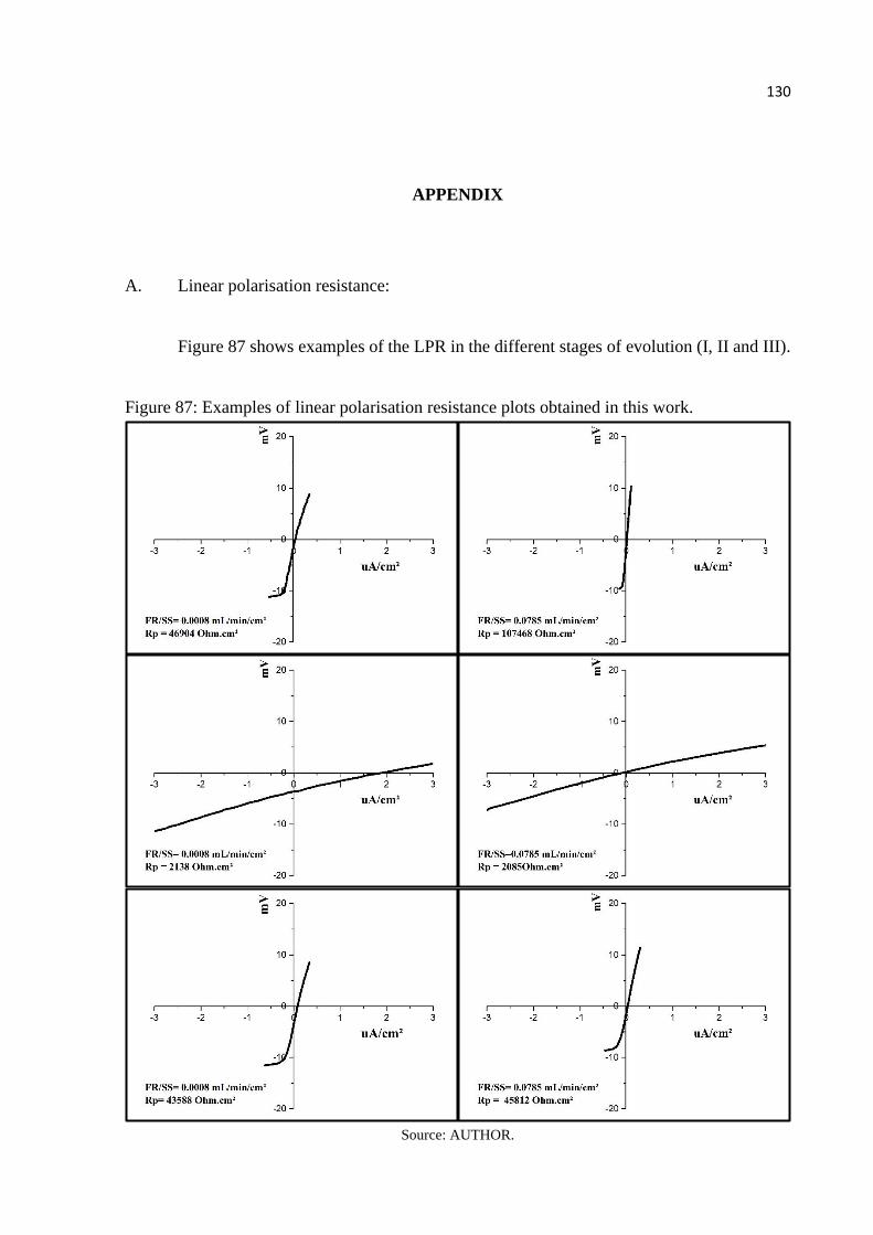
130

APPENDIX

A. Linear polarisation resistance:

Figure 87 shows examples of the LPR in the different stages of evolution (I, II and III).

Figure 87: Examples of linear polarisation resistance plots obtained in this work.

Source: AUTHOR.

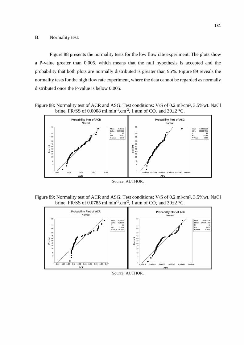
131

B. Normality test:

Figure 88 presents the normality tests for the low flow rate experiment. The plots show

a P-value greater than 0.005, which means that the null hypothesis is accepted and the

probability that both plots are normally distributed is greater than 95%. Figure 89 reveals the

normality tests for the high flow rate experiment, where the data cannot be regarded as normally

distributed once the P-value is below 0.005.

Figure 88: Normality test of ACR and ASG. Test conditions: V/S of 0.2 ml/cm², 3.5%wt. NaCl


Source: AUTHOR.

Figure 89: Normality test of ACR and ASG. Test conditions: V/S of 0.2 ml/cm², 3.5%wt. NaCl


Source: AUTHOR.

0.040.030.020.010.00

99

95

90

80

70

60

50

40

30

20

10

5

1

Mean 0.01773

StDev 0.007609

N 45

AD 0.661

P-Value 0.079

ACR

Perc

en

t

Probability Plot of ACRNormal

0.000450.000400.000350.000300.000250.00020

99

95

90

80

70

60

50

40

30

20

10

5

1

Mean 0.0002669

StDev 0.00004155

N 45

AD 0.583

P-Value 0.122

ASG

Perc

en

t

Probability Plot of ASGNormal

0.070.060.050.040.030.020.010.00-0.01-0.02

99

95

90

80

70

60

50

40

30

20

10

5

1

Mean 0.02125

StDev 0.01800

N 45

AD 3.560

P-Value <0.005

ACR

Perc

en

t

Probability Plot of ACRNormal

0,000560,000480,000400,000320,000240,0001 6

99

95

90

80

70

60

50

40

30

20

1 0

5

1

Mean 0,0003336

StDev 0,0000771 9

N 46

AD 1 ,871

P-Value <0,005

ASG

Perc

en

t

Probability Plot of ASGNormal

132

C. Tolerance interval:

Figure 90 and Figure 91 show the results of the tolerance intervals.

Figure 90: Tolerance intervals of ACR and ASG. Test conditions: V/S of 0.2 ml/cm², 3.5%wt.

NaCl brine, FR/SS of 0.0008 ml.min-1.cm-2, 1 atm of CO2 and 30±2 °C.

Source: AUTHOR.

P-Value 0.079

N 45

Mean 0.018

StDev 0.008

Lower 0.002

Upper 0.033

Lower 0.005

Upper 0.034

94.8%

AD 0.661

Statistics

Normal

Nonparametric

Achieved Confidence

Normality Test

0.0320.0240.0160.0080.000

Nonparametric

Normal

0.030.020.010.00

0.040.030.020.010.00

99

90

50

10

1

Pe

rce

nt

Normal Probability Plot

Tolerance Interval Plot for ACR95% Tolerance Interval

At Least 90% of Population Covered

P-Value 0.122

N 45

Mean 0.000

StDev 0.000

Lower 0.000

Upper 0.000

Lower 0.000

Upper 0.000

94.8%

AD 0.583

Statistics

Normal

Nonparametric

Achieved Confidence

Normality Test

0.000450.000400.000350.000300.000250.00020

Nonparametric

Normal

0.000450.000400.000350.000300.000250.00020

0.000450.000400.000350.000300.000250.00020

99

90

50

10

1

Pe

rce

nt


Tolerance Interval Plot for ASG95% Tolerance Interval


133

Figure 91: Tolerance intervals of ACR and ASG. Test conditions: V/S of 0.2 ml/cm², 3.5%wt.

NaCl brine, FR/SS of 0.0785 ml.min-1.cm-2, 1 atm of CO2 and 30±2 °C.

Source: AUTHOR.

D. Verification of the effect of the geometry of the test vessel

The results of experimental investigations shall not be a function of experimental setups

themselves, but from the studied variables instead. Accordingly, the proximity of the samples

to the inlet nozzle was investigated to observe whether geometry affects or not the ACR and

ASG. Ideally, the corrosion rates and scale growth must remain independent from the test setup.

Bearing that in mind, Figure 92 shows a sketch of the test vessel demonstrating the

identification number and the position of the samples in respect to the inlet nozzle (N). The

sketch shows zone A, closer to the inlet nozzle, zones B and D, at intermediate distances, and

P-Value < 0.005

N 45

Mean 0.021

StDev 0.018

Lower -0.015

Upper 0.058

Lower 0.003

Upper 0.065

94.8%

AD 3.560

Statistics

Normal

Nonparametric

Achieved Confidence

Normality Test

0.0640.0480.0320.0160.000-0.016

Nonparametric

Normal

0.0750.0500.0250.000

0.060.040.020.00-0.02

99

90

50

10

1

Pe

rce

nt


Tolerance Interval Plot for ACR95% Tolerance Interval


134

zone C, further distant from the nozzle. Figure 93.a. shows the results of the ACR analysis,

which reveal similar mean values and amplitudes despite the various distances to the inlet

nozzle. Figure 93.b. show comparable ASG for the zones A, B and C but a considerable

variation for zone D. Such variation is explained by the presence of the sample #02 in the

calculus, once this sample was identified as an outlier (see Table 11), meaning that the variation

of zone D can be disregarded. Therefore, the analysis of the geometry of the test vessel indicates

that the samples corroded in similar atmospheres, independent from the distance to the inlet

nozzle or geometry of the test vessel. Moreover, the result confirms the work of Rubin et al.

(2012) that observed no correlation with the position of the CO2.

Figure 92: A sketch of the test vessel and samples, grouped by the proximity to the inlet nozzle

(N). The working electrodes (WE) are positioned in the centre of the vessel. Zone A

- samples closer to the inlet nozzle. Zones B and D - samples at intermediate distances

to the inlet nozzle. Zone C – samples at the largest distance to the inlet nozzle. Test



Source: AUTHOR.

135

Figure 93: Means and amplitudes of ACR and ASG, in respect to the proximity to the inlet

nozzle. The grey horizontal lines show the tolerance interval. Test conditions: V/S of


30±2 °C.

Source: AUTHOR.

A verification of the proximity of the samples to the inlet nozzle was also carried to

identify if the vessel set up at the high flow rate condition has affected the ACR and ASG

results. Figure 94 shows a sketch of the test vessel demonstrating the identification number and

the position of the samples that were grouped concerning the distance of the inlet nozzle. Figure

95 shows the mean values and amplitudes of the ACR and ASG. As well as observed in the low

flow rate experiments, the means and amplitudes of the results remained similar to each other

despite the distances to the inlet nozzle. Then, this work assumes that all samples were tested

in similar atmospheres, independent from the setup of the test vessel.

a)

b)

136

Figure 94: A sketch of the test vessel and samples, grouped by the proximity to the inlet nozzle

(N). The working electrodes (WE) are positioned in the centre of the vessel. Zone A

- samples closer to the inlet nozzle. Zones B and D - samples at intermediate distances

to the inlet nozzle. Zone C – samples at the largest distance to the inlet nozzle. Test



Source: AUTHOR.

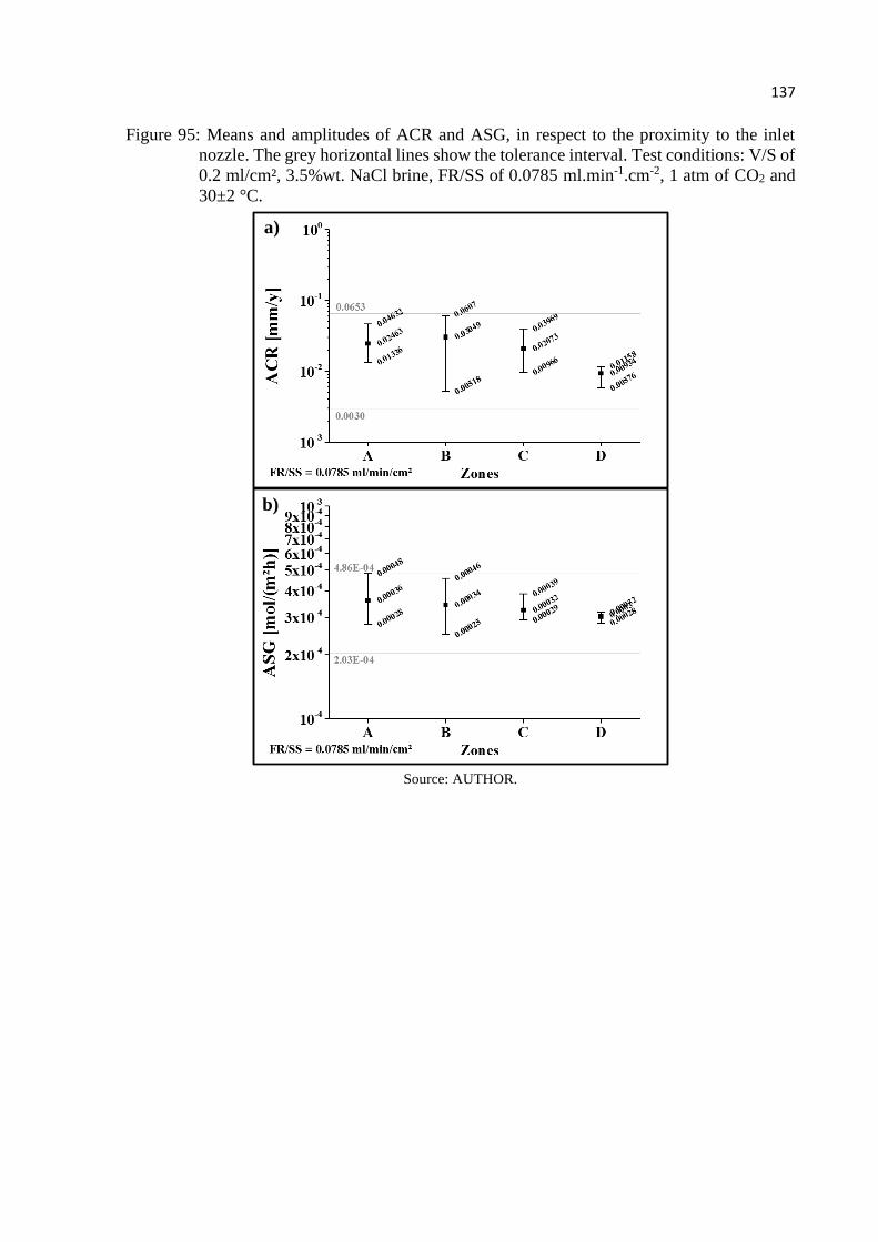
137

Figure 95: Means and amplitudes of ACR and ASG, in respect to the proximity to the inlet

nozzle. The grey horizontal lines show the tolerance interval. Test conditions: V/S of


30±2 °C.

Source: AUTHOR.

a)

b)

Documents

RICARDO FEYH RIBEIRO - UFRGS