Embed Size (px)
Citation preview

Robust and Adaptive NonlinearAttitude Control of a Spacecraft
Guilherme Fragoso Trigo
Dissertação para a obtenção do Grau de Mestre em
Engenharia Aeroespacial
JúriPresidente: Prof. João Manuel Lage de Miranda LemosOrientador: Prof. António Pedro AguiarVogal: Prof. António Manuel Santos Pascoal
Outubro de 2011


Abstract
In the context of the initiative Formation for Atmospheric Science and Technology demonstration(FAST), this dissertation describes the design and comparison of several nonlinear attitude controllers forTU Delft’s micro-satellite. The control requirements include robustness against model uncertainties anddisturbances. To this end, Backstepping is selected as the base control design for the stability awarenessprovided and the versatility in rendering the control law robust and adaptive. Five Backstepping schemesare selected for comparison: Standard Static, Static Robust, Integrated Adaptive with tuning functionsestimation, Modular Adaptive with nonlinear extended state observation and, finally, Immersion andInvariance Adaptive. The spacecraft model is written using Modified Rodrigues Parameters. Threeperturbation sources are considered and applied separately: constant inertia tensor mismatch; saturatedreaction wheel; and moving mirror from a payload spectrometer. All perturbations are translated totime-variant disturbance torques.Convergence of the tuning functions estimator to the true disturbance value is proved. The Immersion
and Invariance Adaptive Backstepping law is here proved input-to-state stable in case of time-variableperturbation. Command filters are used in all designs allowing the inclusion of magnitude and rate con-straints. Simulation reveals similar tracking performances of all controlled systems in a disturbance-freecase. In all disturbance scenarios the adaptive laws clearly outperform the static ones. This is especiallyevident in the presence of a faulty reaction wheel and a moving payload. Sampling time analysis showshigher dependence of the adaptive designs on the control frequency. The Modular Adaptive and theImmersion and Invariance Adaptive Backstepping controllers display the best performances. However,the latter design emerges as, not only the easiest to tune, but also as the one with the most consistentperformance.
Keywords: Spacecraft Attitude Control, Robust Control, Adaptive Control, Backstepping, Immersionand Invariance, Modified Rodrigues Parameters.
i
Resumo
No ambito do projecto Formation for Atmospheric Science and Technology demonstration (FAST), apesquisa apresentada nesta dissertacao descreve o desenvolvimento, teste e comparacao de um conjuntode algoritmos nao-lineares para o controlo de atitude do micro-satelite FAST-D, que sera concebido pelauniversidade de Delft. Os requisitos para o sistema de controlo incluem robustez contra parametrosincertos e perturbacoes. Para tal, o metodo de controlo por Backstepping e escolhido como desenhobase por usar analise de estabilidade em cada passo da deducao da lei de controlo e por ser facilmentetornado robusto e adaptativo. Sao escolhidos cinco algoritmos Backstepping : Standard Static, StaticRobust, Integrated Adaptive com estimacao por Tuning Functions, Modular Adaptive com estimacao porNonlinear Extended State Observer e, finalmente, Immersion and Invariance Adaptive. O modelo de corporıgido e deduzido usando parametros de Rodrigues modificados. Tres tipos de perturbacao (traduzidosnum momento variante no tempo) sao considerados e aplicados separadamente, devendo-se a: erros namedicao das propriedades inerciais; uma roda inercial saturada; e ao movimento de partes mecanicas eminstrumentos.E provada a convergencia da estimativa obtida por Tuning Tunctions para o verdadeiro valor da per-
turbacao variante no tempo. E tambem provada a input-to-state stability do algoritmo Immersion andInvariance em caso de perturbacao variante no tempo. Todos os controladores sao desenvolvidos usandofiltragem dos sinais de comando de forma a incluir limitadores de magnitude e primeira derivada. As si-mulacoes realizadas revelam desempenho semelhante dos cinco controladores na ausencia de perturbacao.Perante cada uma das perturbacoes as leis adaptativas mostram melhor desempenho que as estaticas,sendo tal especialmente evidente nos casos de saturacao de uma roda de inercia e de movimento de partesmecanicas. Os controladores adaptativos revelam uma maior dependencia da frequencia de amostragemdo controlo. Das leis testadas, a Modular Adaptive Backstepping e a Immersion and Invariance AdaptiveBackstepping sao as que apresentam melhor desempenho, sendo, no entanto, a segunda a que revela maiorconsistencia.
Palavras Chave: Controlo de Atitude de Satelite, Controlo Robusto, Controlo Adaptativo, Backstep-ping, Immersion and Invariance, parametros de Rodrigues modificados.
ii
Acknowledgements
Writing a master thesis is a demanding task made easier by the ones who, somehow, help us, supportus or simply inspire us. To them, I owe (more than) a word of gratitude.
Firstly, I would like to thank Dr.ir. Q. P. Chu, who, with his patient guidance and enthusiastic encour-agement, made this dissertation possible. I am grateful to Professor A. P. Aguiar for his support andprompt, though always careful and sharp, revision of my work. I would also like to thank the remainingthesis jury members Prof. J. Miranda Lemos and Prof. A. S. Pascoal.
When we, the Portuguese Aerospace students, arrived in The Netherlands we could not have imaginedthe tremendous amount of people we would meet and how each one of them would make this experienceso special. However, the sun was not always shining and, despite all the obstacles that living and studyingabroad carry, we always knew how to work together and support each other. Now, looking back, I realiseI could never have made it without them. Hugo, Joao, Nuno, Pedro O., Pedro S., Pietro, Tiago a trueand deep thank you.
Finally, I want to express my gratitude to my family that, not only supported me financially duringmy studies, but also always showed me the importance of hard work and perseverance. Their love andcare were my driving force.
A todos o meu sincero obrigado.
Lisboa, Instituto Superior Tecnico Guilherme Fragoso TrigoOctober 27, 2011
iii
Contents
Acronyms ix
1 Introduction 11.1 Background . . . . . . . . . . . . . . . . . . . . . . . . . . . . . . . . . . . . . . . . . . . . 11.2 Research Objectives . . . . . . . . . . . . . . . . . . . . . . . . . . . . . . . . . . . . . . . 11.3 Thesis Outline . . . . . . . . . . . . . . . . . . . . . . . . . . . . . . . . . . . . . . . . . . 2
2 FAST Mission 32.1 Mission Description . . . . . . . . . . . . . . . . . . . . . . . . . . . . . . . . . . . . . . . 32.2 Spacecraft Specifications . . . . . . . . . . . . . . . . . . . . . . . . . . . . . . . . . . . . . 42.3 Attitude Control Objectives . . . . . . . . . . . . . . . . . . . . . . . . . . . . . . . . . . . 5
3 Nominal Spacecraft Model 63.1 Reference Frames . . . . . . . . . . . . . . . . . . . . . . . . . . . . . . . . . . . . . . . . . 63.2 Kinematics . . . . . . . . . . . . . . . . . . . . . . . . . . . . . . . . . . . . . . . . . . . . 6
3.2.1 Modified Rodrigues Parameters . . . . . . . . . . . . . . . . . . . . . . . . . . . . . 83.3 Dynamics . . . . . . . . . . . . . . . . . . . . . . . . . . . . . . . . . . . . . . . . . . . . . 93.4 Gravity Gradient Torque . . . . . . . . . . . . . . . . . . . . . . . . . . . . . . . . . . . . . 103.5 Nominal Model and Implementation . . . . . . . . . . . . . . . . . . . . . . . . . . . . . . 11
3.5.1 Integration Method . . . . . . . . . . . . . . . . . . . . . . . . . . . . . . . . . . . 11
4 Uncertain Spacecraft Model 124.1 Constant Inertial Mismatch . . . . . . . . . . . . . . . . . . . . . . . . . . . . . . . . . . . 124.2 Inner Moving Part . . . . . . . . . . . . . . . . . . . . . . . . . . . . . . . . . . . . . . . . 12
4.2.1 High Speed Disk . . . . . . . . . . . . . . . . . . . . . . . . . . . . . . . . . . . . . 144.2.2 Rotating Cuboid . . . . . . . . . . . . . . . . . . . . . . . . . . . . . . . . . . . . . 15
5 Control of Nonlinear Systems 175.1 Introduction . . . . . . . . . . . . . . . . . . . . . . . . . . . . . . . . . . . . . . . . . . . . 175.2 Control Techniques for Nonlinear Systems . . . . . . . . . . . . . . . . . . . . . . . . . . . 17
5.2.1 Design via Linearization . . . . . . . . . . . . . . . . . . . . . . . . . . . . . . . . . 175.2.2 Gain Scheduling . . . . . . . . . . . . . . . . . . . . . . . . . . . . . . . . . . . . . 185.2.3 Nonlinear Dynamic Inversion . . . . . . . . . . . . . . . . . . . . . . . . . . . . . . 185.2.4 Backstepping . . . . . . . . . . . . . . . . . . . . . . . . . . . . . . . . . . . . . . . 19
5.3 Nonlinear Adaptive Control . . . . . . . . . . . . . . . . . . . . . . . . . . . . . . . . . . . 205.3.1 Schemes for Adaptive Control . . . . . . . . . . . . . . . . . . . . . . . . . . . . . . 205.3.2 On-line Estimation . . . . . . . . . . . . . . . . . . . . . . . . . . . . . . . . . . . . 20
5.4 Design Selection Considerations . . . . . . . . . . . . . . . . . . . . . . . . . . . . . . . . . 23
6 Backstepping Control Design 246.1 Stability Concepts and Lyapunov Theory . . . . . . . . . . . . . . . . . . . . . . . . . . . 24
6.1.1 Lyapunov Stability . . . . . . . . . . . . . . . . . . . . . . . . . . . . . . . . . . . . 246.1.2 Lyapunov’s Direct Method . . . . . . . . . . . . . . . . . . . . . . . . . . . . . . . 266.1.3 Control Lyapunov Functions . . . . . . . . . . . . . . . . . . . . . . . . . . . . . . 27
6.2 Backstepping Design . . . . . . . . . . . . . . . . . . . . . . . . . . . . . . . . . . . . . . . 296.2.1 Integrator Backstepping . . . . . . . . . . . . . . . . . . . . . . . . . . . . . . . . . 296.2.2 Recursive Design for Higher Order Systems . . . . . . . . . . . . . . . . . . . . . . 306.2.3 Command Filtering Backstepping . . . . . . . . . . . . . . . . . . . . . . . . . . . . 31
6.3 Robust Backstepping . . . . . . . . . . . . . . . . . . . . . . . . . . . . . . . . . . . . . . . 32
iv

6.3.1 Nonlinear Damping . . . . . . . . . . . . . . . . . . . . . . . . . . . . . . . . . . . 326.3.2 Recursive Design for Higher Order Systems . . . . . . . . . . . . . . . . . . . . . . 336.3.3 Command Filtering Robust Backstepping . . . . . . . . . . . . . . . . . . . . . . . 34
7 Adaptive Backstepping Design 357.1 Modular Adaptive Backstepping . . . . . . . . . . . . . . . . . . . . . . . . . . . . . . . . 35
7.1.1 Nonlinear Extended State Observer . . . . . . . . . . . . . . . . . . . . . . . . . . 367.2 Integrated Adaptive Backstepping . . . . . . . . . . . . . . . . . . . . . . . . . . . . . . . 37
7.2.1 Integrator Backstepping with Tuning Functions . . . . . . . . . . . . . . . . . . . . 387.2.2 Recursive Design for Higher Order Systems . . . . . . . . . . . . . . . . . . . . . . 397.2.3 Design for Time-varying Uncertainties . . . . . . . . . . . . . . . . . . . . . . . . . 407.2.4 Proof of Estimation Convergence for Disturbed Systems . . . . . . . . . . . . . . . 41
7.3 Command Filtering Adaptive Backstepping . . . . . . . . . . . . . . . . . . . . . . . . . . 427.4 Immersion and Invariance Adaptive Backstepping . . . . . . . . . . . . . . . . . . . . . . . 43
7.4.1 Concept of Immersion and Invariance . . . . . . . . . . . . . . . . . . . . . . . . . 437.4.2 Design for Higher Order Systems . . . . . . . . . . . . . . . . . . . . . . . . . . . . 467.4.3 Time-varying Uncertainties . . . . . . . . . . . . . . . . . . . . . . . . . . . . . . . 497.4.4 Command Filtered I&I Control Design . . . . . . . . . . . . . . . . . . . . . . . . . 50
8 Attitude Controller Designs 518.1 Introduction . . . . . . . . . . . . . . . . . . . . . . . . . . . . . . . . . . . . . . . . . . . . 518.2 Standard Backstepping Controller . . . . . . . . . . . . . . . . . . . . . . . . . . . . . . . 518.3 Robust Backstepping Controller . . . . . . . . . . . . . . . . . . . . . . . . . . . . . . . . . 528.4 Modular Adaptive Backstepping Controller . . . . . . . . . . . . . . . . . . . . . . . . . . 53
8.4.1 Nonlinear Extended State Observer . . . . . . . . . . . . . . . . . . . . . . . . . . 558.5 Integrated Adaptive Backstepping Controller . . . . . . . . . . . . . . . . . . . . . . . . . 568.6 Immersion and Invariance Adaptive Backstepping Controller . . . . . . . . . . . . . . . . 568.7 Gain Selection . . . . . . . . . . . . . . . . . . . . . . . . . . . . . . . . . . . . . . . . . . 58
9 Simulation and Performance Analysis 609.1 Uncertainty Scenarios . . . . . . . . . . . . . . . . . . . . . . . . . . . . . . . . . . . . . . 60
9.1.1 Constant Inertial Mismatch . . . . . . . . . . . . . . . . . . . . . . . . . . . . . . . 609.1.2 Uncontrolled Reaction Wheel . . . . . . . . . . . . . . . . . . . . . . . . . . . . . . 619.1.3 Moving Payload . . . . . . . . . . . . . . . . . . . . . . . . . . . . . . . . . . . . . 62
9.2 Simulated Attitude Trajectory . . . . . . . . . . . . . . . . . . . . . . . . . . . . . . . . . 639.3 Controllers Performance . . . . . . . . . . . . . . . . . . . . . . . . . . . . . . . . . . . . . 64
9.3.1 Nominal Performance . . . . . . . . . . . . . . . . . . . . . . . . . . . . . . . . . . 659.3.2 Constant Inertial Mismatch . . . . . . . . . . . . . . . . . . . . . . . . . . . . . . . 679.3.3 Uncontrolled Reaction Wheel . . . . . . . . . . . . . . . . . . . . . . . . . . . . . . 689.3.4 Moving Payload . . . . . . . . . . . . . . . . . . . . . . . . . . . . . . . . . . . . . 719.3.5 Influence of the Sampling Time . . . . . . . . . . . . . . . . . . . . . . . . . . . . . 73
9.4 Summary of Results . . . . . . . . . . . . . . . . . . . . . . . . . . . . . . . . . . . . . . . 75
10 Conclusions and Recommendations 7710.1 Final Conclusions . . . . . . . . . . . . . . . . . . . . . . . . . . . . . . . . . . . . . . . . . 7710.2 Recommendations . . . . . . . . . . . . . . . . . . . . . . . . . . . . . . . . . . . . . . . . 78
Bibliography 79
A Modified Rodrigues Parameters 83A.1 MRP Kinematics Derivation . . . . . . . . . . . . . . . . . . . . . . . . . . . . . . . . . . . 83A.2 MRP Algebra . . . . . . . . . . . . . . . . . . . . . . . . . . . . . . . . . . . . . . . . . . . 84A.3 MRP Error and Error Rate Derivations . . . . . . . . . . . . . . . . . . . . . . . . . . . . 85A.4 Compensated MRP Tracking Error Approximation . . . . . . . . . . . . . . . . . . . . . . 85
B Boundedness of the Disturbance Torque 86B.1 Norm Tools . . . . . . . . . . . . . . . . . . . . . . . . . . . . . . . . . . . . . . . . . . . . 86B.2 Constant Inertial Mismatch . . . . . . . . . . . . . . . . . . . . . . . . . . . . . . . . . . . 87B.3 Inner Moving Part . . . . . . . . . . . . . . . . . . . . . . . . . . . . . . . . . . . . . . . . 87
v

C Command Filter and Parameter Projection 89C.1 Command Filter . . . . . . . . . . . . . . . . . . . . . . . . . . . . . . . . . . . . . . . . . 89C.2 Parameter Projection . . . . . . . . . . . . . . . . . . . . . . . . . . . . . . . . . . . . . . 91
D MRP Reference Building 93D.1 Reorientation Maneuver . . . . . . . . . . . . . . . . . . . . . . . . . . . . . . . . . . . . . 93D.2 Scanning Maneuver . . . . . . . . . . . . . . . . . . . . . . . . . . . . . . . . . . . . . . . . 94
E Additional Plots 95E.1 Nominal Scenario . . . . . . . . . . . . . . . . . . . . . . . . . . . . . . . . . . . . . . . . . 96E.2 Constant Inertial Mismatch . . . . . . . . . . . . . . . . . . . . . . . . . . . . . . . . . . . 98E.3 Uncontrolled Reaction Wheel . . . . . . . . . . . . . . . . . . . . . . . . . . . . . . . . . . 100E.4 Moving Payload . . . . . . . . . . . . . . . . . . . . . . . . . . . . . . . . . . . . . . . . . . 102
vi

List of Figures
2.1 FAST-D satellite preliminary design (Guo, Maessen, Gill, Moon, & Zheng, 2009). . . . . . 42.2 FAST-D payload instruments: SPEX and SILAT (Maessen, Guo, Gill, Gunter, et al., 2009). 4
3.1 View of LVLH and Body reference frames. . . . . . . . . . . . . . . . . . . . . . . . . . . . 7
4.1 Rigid body with a moving part. . . . . . . . . . . . . . . . . . . . . . . . . . . . . . . . . . 134.2 Rotating disk inside the spacecraft’s body. . . . . . . . . . . . . . . . . . . . . . . . . . . . 144.3 Rotating cuboid inside the spacecraft’s body. . . . . . . . . . . . . . . . . . . . . . . . . . 15
6.1 Lyapunov stability in R2. . . . . . . . . . . . . . . . . . . . . . . . . . . . . . . . . . . . . 25
6.2 State x evolution (top) and control effort u (bottom) using Full and Partial linearizationcontrollers. . . . . . . . . . . . . . . . . . . . . . . . . . . . . . . . . . . . . . . . . . . . . 29
7.1 Nonlinear gain compared to the linear one for α = 1. . . . . . . . . . . . . . . . . . . . . . 377.2 State regulation, control effort and parameter estimation evolutions of the tuning function
adaptive controller and the I&I adaptive design. . . . . . . . . . . . . . . . . . . . . . . . 46
9.1 Reaction wheel configuration (Bakker, 2009). . . . . . . . . . . . . . . . . . . . . . . . . . 619.2 Moving mirror (part b). . . . . . . . . . . . . . . . . . . . . . . . . . . . . . . . . . . . . . 639.3 Attitude reference trajectory. . . . . . . . . . . . . . . . . . . . . . . . . . . . . . . . . . . 649.4 Pointing angular error θe of all control laws in the nominal scenario. . . . . . . . . . . . . 669.5 Rate error norm of all control laws in the nominal scenario. . . . . . . . . . . . . . . . . . 669.6 Pointing error θe of all control laws in the presence of constant inertial mismatch. . . . . . 689.7 Rate error norm for all controllers in the presence of constant inertial mismatch. . . . . . 689.8 Angular pointing error θe in the presence of a saturated RW. . . . . . . . . . . . . . . . . 709.9 Rate error norm in the presence of saturated RW. . . . . . . . . . . . . . . . . . . . . . . 709.10 Pointing error θe in the presence of moving payload. . . . . . . . . . . . . . . . . . . . . . 729.11 Rate error norm in the presence of moving payload. . . . . . . . . . . . . . . . . . . . . . 73
C.1 Command filter design with magnitude and rate limiters (Farrell, Polycarpou, & Sharma,2004). . . . . . . . . . . . . . . . . . . . . . . . . . . . . . . . . . . . . . . . . . . . . . . . 89
C.2 Command filter magnitude saturated output (left plot) and rate saturated output (rightplot). . . . . . . . . . . . . . . . . . . . . . . . . . . . . . . . . . . . . . . . . . . . . . . . . 90
E.1 Angular parameter and rate tracking in the nominal scenario. . . . . . . . . . . . . . . . . 96E.2 Applied control torque and disturbance torque estimation in the nominal scenario. . . . . 97E.3 Angular parameter and rate tracking in the presence of a constant inertial mismatch. . . . 98E.4 Applied control torque and disturbance torque estimation in the presence of a constant
inertial mismatch. . . . . . . . . . . . . . . . . . . . . . . . . . . . . . . . . . . . . . . . . 99E.5 Angular parameter and angular rate tracking in the presence of a saturated RW. . . . . . 100E.6 Applied control torque and disturbance torque estimation in the presence of a saturated
RW. . . . . . . . . . . . . . . . . . . . . . . . . . . . . . . . . . . . . . . . . . . . . . . . . 101E.7 Angular parameter and rate tracking in the presence of moving payload. . . . . . . . . . . 102E.8 Applied control torque in the presence of moving payload. . . . . . . . . . . . . . . . . . . 103E.9 NESO rate estimation error (innovation) in the presence of moving payload. . . . . . . . . 103E.10 Disturbance torque estimation in the presence of moving payload. . . . . . . . . . . . . . . 104
vii

List of Tables
2.1 Orbital parameters of the mission (Maessen, Guo, Gill, Laan, et al., 2009). . . . . . . . . . 32.2 FAST-D preliminary specifications (Maessen, Guo, Gill, Gunter, et al., 2009). . . . . . . . 52.3 Attitude control requirements (Bakker, 2009). . . . . . . . . . . . . . . . . . . . . . . . . . 5
9.1 Reaction Wheels Specifications (Bakker, 2009). . . . . . . . . . . . . . . . . . . . . . . . . 619.2 Reaction wheels position for l = 0.3m. . . . . . . . . . . . . . . . . . . . . . . . . . . . . . 629.3 Possible Euler angles from B to A′ with 3-2-1 rotation order. . . . . . . . . . . . . . . . . 629.4 Mirror (part b) properties. . . . . . . . . . . . . . . . . . . . . . . . . . . . . . . . . . . . . 639.5 Limits imposed on the input signals and estimated states. . . . . . . . . . . . . . . . . . . 659.6 Angular pointing error RMS θeRMS
in the nominal scenario. . . . . . . . . . . . . . . . . . 669.7 Workload along the entire trajectory in the nominal scenario. . . . . . . . . . . . . . . . . 669.8 Angular pointing error RMS θeRMS
in the presence of constant inertial mismatch. . . . . . 689.9 Estimation error RMS during scanning motion for t ∈ [505, 1100] s in the presence of
constant inertial mismatch. . . . . . . . . . . . . . . . . . . . . . . . . . . . . . . . . . . . 689.10 Workload along the entire trajectory in the presence of constant inertial mismatch. . . . . 689.11 Angular pointing error RMS θeRMS
in the presence of a saturated RW. . . . . . . . . . . . 699.12 Estimation error RMS during scanning motion for t ∈ [505, 1100] s in the presence of a
saturated RW. . . . . . . . . . . . . . . . . . . . . . . . . . . . . . . . . . . . . . . . . . . 719.13 Workload along the entire trajectory in the presence of a saturated RW. . . . . . . . . . . 719.14 Angular pointing error RMS θeRMS
in the presence of moving payload. . . . . . . . . . . . 729.15 Estimation error RMS during scanning motion for t ∈ [505, 1100] s in the presence of
moving payload. . . . . . . . . . . . . . . . . . . . . . . . . . . . . . . . . . . . . . . . . . 739.16 Workload along the entire trajectory in the presence of moving payload. . . . . . . . . . . 739.17 Angular pointing error RMS θeRMS
[arcsec] in the presence of a saturated RW for differentsimulation frequencies. Ratio to RMS value at 10Hz shown in brackets. . . . . . . . . . . 74
9.18 Angular pointing error RMS θeRMS[arcsec] in the presence of moving payload for different
simulation frequencies. Ratio to RMS value at 10Hz shown in brackets. . . . . . . . . . . 759.19 Estimation error RMS ratio to total disturbance RMS (TdRMS
/TdRMS) for t ∈ [505, 1100] s
at several frequencies in both scenarios. Ratio to the value at 10Hz in brackets. . . . . . 75
C.1 Saturation sets limits. . . . . . . . . . . . . . . . . . . . . . . . . . . . . . . . . . . . . . . 91C.2 Projection sets. . . . . . . . . . . . . . . . . . . . . . . . . . . . . . . . . . . . . . . . . . . 92
viii

Acronyms
ACS Attitude Control System.
AFCS Automatic Flight Control System.
CLF Control Lyapunov Function.
ESA European Space Agency.
FAST Formation for Atmospheric Science and Technology demonstration.
FAST-D Delft’s FAST Satellite.
FBL Feedback Linearization.
GNC Guidance, Navigation and Control.
I&I Immersion and Invariance.
ISS Input-to-State Stability.
LEO Low Earth Orbit.
LVLH Local-Vertical Local-Horizontal.
MRP Modified Rodrigues Parameters.
NDI Nonlinear Dynamic Inversion.
NESO Nonlinear Extended State Observer.
RMS Root Mean Square.
RW Reaction Wheel.
ix

List of Symbols
Greek Symbols
α∗ Virtual control
β Continuously differentiable function
γ, Γ Estimation gain (scalar or matrix)
∆t Sampling time
η Off-the-manifold coordinate
θ Rotation angle
θ Uncertain parameter
θe Pointing error (angle)
θ Parameter estimate
θ Parameter estimation error
κ Nonlinear damping gain
σ Modified Rodrigues parameter vector
σe Modified Rodrigues parameters error vector
σr Modified Rodrigues parameters reference vector
ϕ Regressor function
χ∗ Filter states
ω Angular velocity
ωb Angular velocity of the spacecraft’s moving part b
Roman Symbols
B Body reference frame
C∗ Direction cosine matrix
c∗ Control gain (scalar or matrix)
c∗ Direction cosine column vector
H Total angular momentum
I Inertial reference frame
J Real spacecraft inertia tensor
J0 Modeled spacecraft inertia tensor
Jb Moving part b inertia tensor
∆J Inertia tensor error
k Rotation axis defining vector
x

M Sum of all applied moments
n Orbital angular velocity
N Kinematics matrix
O LHLV (orbital) reference frame
q Quaternion vector
q Vector composed of the three first quaternion parameters
q1, q2, q3, q4 Quaternion parameters
Sv Skew symmetric matrix of the vector v
T c Control torque
T d Disturbance torque
T d Estimated disturbance torque
T d Disturbance torque estimation error
T g Gravity gradient induced torque
u System control input
V (Control) Lyapunov function
x System state vector
x∗ System state
yr
Reference signal
z∗ Tracking error
z∗ Compensated tracking error
xi

Notation
Vectors and Vector Operations
The vectors will be represented by an underlined lower-case letter (Roman or Greek), for example: vExceptions to this rule are physical quantities that are typically expressed by an upper-case letter, e.g.,
torque (T ) or angular momentum (H). Other two exceptions are made for quaternion representation: thefull quaternion vector is simply q and the vector containing only the three first quaternion parameters iswritten q, none of these is expressed as q.Vectors will always be defined as column matrices:
v =
v1v2v3
For space saving it can as well be written: v =[v1 v2 v3
]Tor vT =
[v1 v2 v3
]
The dot product operation (·) will regularly be expressed using the transpose vector as:
v · u = vTu = uT v
The l2 norm of v (or its length), expressed as |v| or ‖v‖ is defined as: |v| = √v · v
The maximum or l∞ norm will be represented as: ‖v‖∞ = supi≥1
|vi|
The cross product operation (×) will usually be replaced by a matrix representation using skew sym-metric matrices:
v × u = Svu ,
where the skew symmetric matrix Sv is given by:
Sv =
0 −v3 v2v3 0 −v1−v2 v1 0
Matrices
Matrices will be represented using upper-case (Roman or Greek) letters, e.g.: AThe transpose matrix will, as common practice, be written as: AT
As for the inverse matrix, it will be expressed as: A−1
Although the determinant of A may be represented by |A|, here, to avoid confusion with the absolutevalue or the length operators, it will be expressed as: det(A)
Reference Frames
The frames of reference are usually expressed as an upper-case calligraphic letter, such as: IIf it is necessary to stress that a vector is expressed in coordinates of I, it is done as:
(v)I =[v1 v2 v3
]T
I
If we refer to a quantity of I, for example its angular velocity, we write: ωI =[vI1 vI2 vI3
]T
Furthermore, if this quantity is defined with respect to another reference frame B it is expressed as ωIB
and it is read “the angular velocity of the reference frame I with respect to B”.This notation will be used often to write transformation matrices between reference frames. For exam-
ple, CBI is the direction cosine matrix from reference frame B to I.Finally, a time derivative of a quantity v with respect to a frame I is written:
Id
dtv
xii

Chapter 1
Introduction
This chapter presents the dissertation background and places it in the context of the Formationfor Atmospheric Science and Technology demonstration (FAST) initiative. The main researchgoals are defined and the outline of the report is described.
1.1 Background
Since the launch of the first satellite in 1957, the technology behind space vehicles has leaped forward ata large pace. On-board systems gained complexity as requirements became tighter. Attitude control wasnot an exception and passiveness gave place to active and precise pointing. The accuracy of such systemsgrew considerably with the introduction of electric actuators such as reaction wheels and control momentgyroscopes. Today, pointing can be performed with a precision higher than a hundredth of an arcsecond.However, an increasing demand for smaller and lighter satellite designs makes the topic of disturbancerobustness and fault-tolerance more important than ever. Despite the tremendously fast evolution in at-titude control technologies, there is still conservativeness in what comes to control algorithms. Although,especially since the 1960s, the nonlinear control theory has seen extensive developments, very few of itspotential has been used for practical attitude control applications. The lower risk of space-proven lineardesigns is instead chosen with loss of performance, versatility and even fault-tolerance. Such featureshave compromised many satellite missions in the past, as described in (Robertson & Stoneking, 2003).According to the author, wheel anomalies are one of the most common Guidance, Navigation and Control(GNC)-related failures. For instance, Iridium 42 satellite failed due to a faulty wheel tachometer, whichled to uncertain real actuation and thus dramatic attitude control performance loss.In 2007, Delft University of Technology and Beijing’s Tsinghua University joined efforts and started the
Formation for Atmospheric Science and Technology demonstration (FAST). For having a strong academiccomponent, this project will allow the experimentation of recent and developing technologies. One ofthose novelties will lie on the Attitude Control System (ACS) as the attitude of Delft’s FAST Satellite(FAST-D) will be steered by a nonlinear control algorithm.
1.2 Research Objectives
As a follow up of the research done in (Bakker, 2009) concerning the nonlinear control design forthe FAST mission, this dissertation takes control robustness and fault-tolerance to a higher level. Theobjectives of this thesis are:
• Formulate and deduce a set of possible inertial-related disturbances affecting the spacecraft rigid-body model. Implement numerical simulation code of the derived perturbed spacecraft modelsusing Matlab.
• Investigate possible robust and adaptive nonlinear control techniques suitable for precise attitudecontrol of the deduced model. Design and compare through numerical simulation the selectedcontrol laws in the presence of each conceived disturbance scenario.
These goals can be synthesized in one main objective: Design an attitude controller capable of steeringthe spacecraft in an efficient manner in the presence of severe inertial-related disturbances.
1
1.3 Thesis Outline
This dissertation is composed by the following three parts:
• It begins by briefly introducing the FAST mission in Chapter 2. Here the main mission goalsare presented along with the FAST-D spacecraft specification and attitude control system require-ments. In Chapter 3 the nominal spacecraft rigid-body model is deduced using a Modified Ro-drigues Parameters angular representation and including gravity gradient torque. This is followed,in Chapter 4, by the introduction and modeling of several attitude disturbance sources.
• Then, Chapter 5 presents a short survey of control techniques, adaptive schemes and distur-bance/uncertainty estimators for nonlinear systems. Backstepping control design, being the se-lected technique, is explained in detail together with a robustness-added design in Chapter 6.Due to the uncertain nature of the problem at hand, in Chapter 7, several adaptive backstep-ping schemes are described, namely: modular adaptive backstepping, integrated tuning functionsadaptive backstepping and immersion and invariance adaptive backstepping.
• Finally, in Chapter 8 the described control laws, static and adaptive, are implemented to thenominal spacecraft model so then, in Chapter 9, after describing in detail the simulation scenarios,are tested and compared in the presence of three different disturbance sources. In this chapter, thedesigned controllers are also evaluated using various sampling times.
2

Chapter 2
FAST Mission
This chapter briefly describes the FAST mission, specifying the main scientific goals, the missionphases and the chosen orbital parameters. The spacecraft design specifications and attitudecontrol system requirements are presented for the mission’s Dutch satellite, FAST-D.
2.1 Mission Description
The FAST mission is a Dutch-Chinese collaboration project between Delft University of Technology,The Netherlands and Tsinghua University, Beijing, China. The name FAST stands for Formation forAtmospheric Science and Technology demonstration. The project was officially started on December 2007and will include the concept, assembly, launch and operation of two micro-satellites, FAST-D and FAST-T, each conceived by one university (Maessen, Guo, Gill, Laan, et al., 2009). The mission intends notonly to provide atmospheric data, but also to demonstrate cutting-edge technology and to educate. Thefollowing goals are, in the mission concept, equally important (Guo et al., 2009):
• Demonstrate Autonomous Formation Flying using various communication architectures with dis-tributed propulsion systems;
• Characterize atmospheric aerosols, monitor the variation of height profiles in the cryosphere, andcorrelate these data for improved scientific return1;
• Teach cutting-edge technology, broaden the international view of students and boost skills throughthe exchange of students and staff.
The orbital operations will last 2.5 years and will be primarily oriented towards the collection ofatmospheric data.To fulfill the mission objectives the two satellites will fly in formation in an orbit defined by the
parameters on Table 2.1.
Table 2.1: Orbital parameters of the mission (Maessen, Guo, Gill, Laan, et al., 2009).
Type Sun-synchronous Low Earth Orbit (LEO)
Height 650 km
Inclination 98.7 deg
Local time of ascending node 10:00 hours
The formation flight will be carried out in two different phases: A and B. Phase A is divided intoA1, where the two spacecraft will fly with an along-track separation of 1 ± 0.1 km, and A2, where theseparation will be increased to 900 ± 10 km. In Phase B the separation will be even larger and time-defined, in order to study the time evolution of the aerosol levels overtime in a specific site, for examplevariations in an industrial area between morning and afternoon.
1For a more detailed overview of the scientific goals of the project please refer to (Gill, Maessen, Laan, Kraft, & Zheng,2010).
3

Figure 2.1: FAST-D satellite preliminary design (Guo et al., 2009).
(a) SPEX (b) SILAT
Figure 2.2: FAST-D payload instruments: SPEX and SILAT (Maessen, Guo, Gill, Gunter, et al., 2009).
The FAST-D spacecraft (Figure 2.1), designed by TU Delft, will carry two payload Dutch-conceivedscientific instruments: SPEX (Spectropolarimeter for Planetary Exploration) and SILAT (Stereo ImagingLaser Altimeter). SPEX (Figure 2.2(a)) is a 2Kg instrument that measures flux and polarization overa broad wavelength region (400 − 800nm) with a spectral resolution of about 2nm (Laan, 2009). It isunder development by Dutch Space, TNO, SRON (Netherlands Institute for Space Research), ASTRON(Netherlands Foundation for Research in Astronomy) and the Astronomy Department of the Universityof Utrecht. As for SILAT (Figure 2.2(b)), it is a setup with a laser altimeter (LAT) and high-resolution(HRC) and stereo (SCAM) cameras that was first designed for use in planetary exploration missions toMercury and Europa (Moon et al., 2008). For its small size and mass (8Kg) it was converted for Earthobservation on-board of a micro-satellite, in this case, FAST-D. It is developed by Cosine Research BVin Leiden, The Netherlands.
2.2 Spacecraft Specifications
The FAST-D micro-satellite shall have the cuboid design displayed in Figure 2.1. Its preliminaryspecifications are presented in Table 2.2.The specifications for each sensor and actuator are given in detail in (Bakker, 2009). As this thesis
does not cover the theme of state Kalman filtering and control allocation this information is omitted.However, the reaction wheel configuration and characteristics will be used, and therefore referred, furtheron in this dissertation.
2Assuming constant mass density.
4

Table 2.2: FAST-D preliminary specifications (Maessen, Guo, Gill, Gunter, et al., 2009).
Dimensions 0.5× 0.5× 0.7m3
Mass 50Kg
Inertia tensor in the principal axes2
3.083 0 00 3.083 00 0 2.083
Kgm2
Available Attitude Sensors Earth horizon sensorFine and coarse sun sensorsAutonomous star tracker3-axis magnetometer3-axis rate sensor
Available Attitude Actuators 4 Reaction wheels3 Magnetic torquers
2.3 Attitude Control Objectives
The spacecraft’s attitude shall be controlled by a 3-axis tracking control system. Additionally, thedescribed scientific instruments carried by FAST-D require, for data collection, that the attitude controlsystem meets the requirements on Table 2.3.
Table 2.3: Attitude control requirements (Bakker, 2009).
Operating Orientation Near Nadir pointing
Pointing accuracy 30 arcsec (0.0083 deg)
Pointing stability 1 arcsec/s (0.00028 deg/s)
Furthermore, the choice and design of control law and angular representation should meet robustnessto disturbances and design uncertainties and provide easy definition of energy-wise optimal trajectoriesfor attitude maneuvering.
5

Chapter 3
Nominal Spacecraft Model
In this chapter the rigid-body spacecraft model is deduced: the reference frames used are firstdescribed; the kinematics equation is derived for Modified Rodrigues Parameters angular repre-sentation; and the dynamics model is then presented including the gravity induced torque. Thechapter closes with a commentary section on the model implementation.
3.1 Reference Frames
No mechanics system derivation can be done efficiently without a careful choice of reference frames. Forthe spacecraft model deduction three will be used: Inertial, Local-Vertical Local-Horizontal and BodyFixed.
Inertial reference frame (I), also known as Newtonian frame, is a reference with no accelerations, i.e.,it has no motion either than constant rectilinear. Since in this frame of reference there are nofictitious forces the angular quantities and accelerations measured with respect to it are calledabsolute quantities.
Local-Vertical Local-Horizontal (LVLH) reference frame (O) is defined as being centered in thecenter of mass of the orbiting body and having the axes oriented as: the third axis is pointingnadir ; the second is perpendicular to the orbital plane and is defined in the negative direction ofthe orbital velocity vector; and the first axis is defined so that the frame is right-handed1.
Body Fixed reference frame (B) is, as the name says, fixed to the body of the spacecraft. Its centeris defined coincident to the body’s center of mass and its axes are oriented in the directions ofthe principal inertial axes. This alignment, by Sylvester’s law of inertia, renders a diagonal inertiamatrix in this reference frame.
The last two reference frames (see Figure 3.1) are used to define the attitude problem, since theorientation of the body frame with respect to the LVLH frame is the spacecraft’s attitude that is to becontrolled. In nadir pointing attitude the two frames are completely aligned.
3.2 Kinematics
The kinematics describes the motion of a body with respect to the velocities. In the case of the attitudemodel only the rotational motion is considered.Defining the attitude parameter vector that describes the attitude of the body reference frame B
relatively to the LVLH frame O as α, the kinematics equation can be written as
α = N(α)ωBO, (3.1)
where ωBO is the angular velocity of the body frame B relatively to the LVLH frame O and N(α) is thekinematics matrix given in terms of α.
1In a circular orbit the first axis is coincident with the body’s velocity vector.
6

e
B
O
e
e
e
e
eB
B
O
O
1
1
2
2
3
3
Figure 3.1: View of LVLH and Body reference frames.
Considering that the orbital frame rotates with a rate n =[0 −n 0
]Twritten in its own coordinates,
the following relation between angular velocity vectors holds
ωBO = ωBI − COB(α)n
= ωBI + nc2(α) (3.2)
ωBI is the angular velocity of the body with respect to the inertial frame I. COB(α) is the directioncosine matrix that defines the transformation of a vector from the orbital frame to the body frame. Forsimplicity, this matrix will, from here on, be referred to as C. c2(α) is the second column of C.The kinematics expression (3.1) can then be written as
α = N(α)(ωBI + nc2(α)
)(3.3)
This is the basic form of the kinematics equation in terms of a general angular parameter vector.An important tool in deriving N(α) will now be presented. For this, consider a vector v written in
body frame coordinates. The time derivative of v with respect to the LVLH reference frame O can becomputed by first transforming it to O, taking its time derivative and then transforming it back to B,that is
Od
dtv =C
d
dt(CT v) = CCT
Bd
dtv + CCT v
=Bd
dtv + CCT v , (3.4)
where the property C−1 = CT ⇒ CCT = I was used.This is nothing more than the transport theorem written in vector algebra as (Schaub & Junkins, 2002)
Od
dtv =
Bd
dtv + ωBO × v (3.5)
Comparing (3.4) with (3.5) the following relation is revealed
CCT = ωBO× = SωBO , (3.6)
where SωBO is a skew symmetric matrix of SωBO .Rearranging (3.6) gives
(CCT )T =(SωBO
)T
CCT = −SωBO
C = −SωBOC (3.7)
(3.7) is known as Poisson’s kinematic differential equation for the direction cosine matrix (Schaub,Tsiotras, & Junkins, 1995). From this differential equation it is possible to derive the kinematics matrixN(α).
7

3.2.1 Modified Rodrigues Parameters
The Modified Rodrigues Parameters (MRP) are a three component angular representation obtained bystereographic projection2 of the quaternion (Euler-Rodrigues) parameters. This transformation createssingularities at ±360 deg, which is much more practical then the ±180 deg singularities in the ClassicalRodrigues Parameters, carrying the same 3-parameter representation advantages. Moreover, the MRPangular representation behaves linearly in a domain eight times larger than the Classical Rodriguesparameters. In fact, in (Junkins & Singla, 2004) the authors claim, based on numerical analysis, thatthe modified Rodrigues parameters are the most linearly behaving three-component attitude parameters,having a close performance to quaternion parameters with the advantage of using only three components.This was the reason why this representation was chosen for this project.The modified Rodrigues parameters exist in two forms: the positive form and the negative form (Shuster,
1993). These forms depend on which pole of the sphere is chosen as the infinity point of the stereographicprojection (1 or North in the positive form and -1 or South in the negative one). The most commonlyused is the positive form, which gives the MRP vector σ in terms of quaternion parameters as (Tsiotras,1994)
σ =q
1 + q4(3.8)
where q is a vector composed of the three first quaternion parameters and q4 is the forth. The quaternionparameters can be directly given from the Euler angle-axis rotation representation as (Hanson, 2006)
q =
[qq4
]
=
[k sin
(θ2
)
cos(θ2
)
]
(3.9)
where k is the unit-vector that defines the axis of (right-hand) rotation and θ is the angle of such rotation.The MRP vector σ can be also given in terms of this angle-axis notation by
σ =k sin
(θ2
)
1 + cos(θ2
) (3.10)
which, by basic trigonometry relations, yields
σ = k tan
(θ
4
)
(3.11)
In (3.11) it is obvious the singularity in θ/4 = ±90 deg ⇒ θ = ±360 deg. This feature of the MRPconstrains the rotations to |θ| < 360 deg, which is for most practical cases a wide-enough rotation range.Nevertheless, a way of overcoming this problem and allowing for more than one cycle rotations is to usethe shadow parameter. It is defined as (Radice & Casasco, 2007)
σs = − σ
|σ|2 (3.12)
and, similarly to the quaternion image points (q and q−1), these two parameters describe the same physicalorientation as well. What makes the shadow parameter useful is that its singularities are 360 deg apartfrom the ones of σ. Whereas the original parameter is close to linear near the origin and singular at±360 deg, the shadow parameter behaves linearly at ±360 deg and singularly near the origin. Theuse of the shadow parameter becomes obvious: when a singularity is reached all it takes to avoid it isswitch to the shadow of the current attitude. This is possible because the two parameters have the samekinematics equation, differing only in the initial condition. The switching point can be chosen anywherewithin ±360 deg, being typically at ±180 deg where |σ|2 = 1 (Schaub & Junkins, 1996). In addition, inthis region the MRP behave almost linearly making the attitude control task easier.To derive the direction cosine matrix from the Body reference frame B to the LVLH reference frame
O in terms of MRP, consider first the Rodrigues rotation formula in its most common form (Goldstein,Poole, & Safko, 2002)
v′ = v cos(θ) + k(kT v) (1− cos(θ)) + (v × k) sin(θ) (3.13)
where v is rotated an angle θ (right-hand direction) around the axis defined by k, becoming v′. Theexpression (3.13) can be rearranged to a matrix-times-vector form as
C(k, θ)v′ =[
I cos(θ) + kkT (1− cos(θ))− Sk sin(θ)]
v (3.14)
2This transformation, which is widely used in geographical globe mapping, projects the points of a spherical surface ontoa plane that is defined tangent to it (Coxeter, 1969).
8

To arrive at the direction cosine matrix in terms of MRP it is easier to first write it using quaternionparameters. For that the following relations are useful
q =
[qq4
]
=
[
k sin(θ2
)
cos(θ2
)
]
⇒
k =q
√
1− q24
cos(θ) = 2q24 − 1
sin(θ) = 2q4√
1− q24
(3.15)
Using (3.15) in (3.14) and the vector property
qqT = S2q + qT qI (3.16)
yieldsC(q, q4) = I − 2q4Sq + 2S2
q (3.17)
Now relating the quaternion parameters with the MRP by
q =2σ
1 + |σ|2 , q4 =1− |σ|21 + |σ|2 (3.18)
it is possible to give (3.17) in terms of MRP
C(σ) = I − 4(1− |σ|2)(1 + |σ|2)2 Sσ +
8
(1 + |σ|2)2S2σ (3.19)
or in explicit matrix form
C(σ) =1
(1 + |σ|2)2
(1 + |σ|2)2 − 8σ22 − 8σ2
3 8σ1σ2 + 4σ3(1− |σ|2) 8σ1σ3 − 4σ2(1− |σ|2)8σ1σ2 − 4σ3(1− |σ|2) (1 + |σ|2)2 − 8σ2
1 − 8σ23 8σ2σ3 + 4σ1(1− |σ|2)
8σ1σ3 + 4σ2(1− |σ|2) 8σ2σ3 − 4σ1(1− |σ|2) (1 + |σ|2)2 − 8σ21 − 8σ2
2
(3.20)The kinematics equation in terms of MRP is easily derived from the quaternion parameters kinematics,
as it is done in Appendix A.1, and is given in the form of (3.3) by
σ = N(σ)ωBO =1
4
[(1− |σ|2)I + 2Sσ + 2σσT
] (ωBI + nc2(σ)
)(3.21)
3.3 Dynamics
A spacecraft can be viewed as a small mass orbiting a much heavier one. In the present case the centerbody is the Earth and the orbit is considered circular. This means that the orbital angular velocity n isconstant throughout one complete cycle.In a rigid-body, the sum of all applied moments M equals the time derivative of the angular momentum
about the center of mass with respect to the inertial reference frame I (Wie, 2008)
Id
dtH = M , (3.22)
where the total angular momentum H about the center of mass of the rigid-body is given by
H = JωBI (3.23)
For ease of notation the body’s total angular velocity ωBI will from here on be written as ω. Themoment of inertia matrix J is diagonal by proper definition of the body reference frame B. It is writtenas
J =
J1 0 00 J2 00 0 J3
(3.24)
Using (3.23) the time derivative of the total angular moment in (3.22) can be given with respect to Bas
M =Id
dtH =
Bd
dtH + ω ×H =
Bd
dt(Jω) + ω × Jω = Jω + SωJω , (3.25)
9
Sω is a skew symmetric matrix of ω.The total moment applied M can be split into several moments as
M = T g + T c + T d , (3.26)
where T g is the gravity gradient torque, T c is the control (actuator) torque and T d is the disturbancetorque, that can be due, for example, to aerodynamic drag, magnetic induced torque or moving parts.Combining (3.25) and (3.26) yields the dynamics equation
Jω = −SωJω + T g + T c + T d (3.27)
3.4 Gravity Gradient Torque
A spacecraft orbiting a planet experiences a torque resultant from the slight difference of gravity forcealong its body caused by the gravity field’s nonuniformity.The gravitational acceleration due to Earth’s mass at a point in space is computed as (Wiesel, 1997)
g = −GM⊕|r|3 r (3.28)
where G is the gravitational constant, M⊕ is the Earth’s mass and r is the position vector of the selectedpoint with respect to Earth’s center of mass.If we select a mass point dm of the spacecraft’s body, r can be written as
r = R+ d, (3.29)
with R being the vector between the centers of mass of the central and orbiting bodies and d being theposition vector of point dm with respect to the center of mass of the spacecraft.The torque caused by the gravity gradient across the spacecraft is given by
T g =
∫
Bd× g dm (3.30)
Assuming that the spacecraft is small compared to the distance |R| the following approximation canbe made
1
|r|3 =1
|R+ d|3 =1
(|R|2 + 2R · d+ |d|2) 3
2
≈ 1
|R|3(1 + 2|R|2R · d+ . . . )
3
2
≈ 1
|R|3(
1− 3
|R|2R · d)
(3.31)
where the last relation was obtained using the binomial approximation and neglecting the second andhigher order terms.Using the approximation (3.31) in (3.30) gives:
T g = −GM⊕
∫
Bd× R+ d
|R|3(
1− 3
|R|2R · d)
dm =GM⊕|R|3 R×
(∫
Bd dm− 3
|R|2∫
Bd(R · d)dm
)
(3.32)where the property d× d = 0 was used. Knowing that d is measured with respect to the center of mass,then
∫
B d dm = 0, yielding
T g =3GM⊕|R|5 R×
∫
B−d(R · d)dm (3.33)
Using the identity a× (b× c) = b(a · c)− c(a · b) in (3.33) gives
T g =3GM⊕|R|5 R×
∫
B(−d× (d×R)−R(d · d)) dm
=3GM⊕|R|5
(
−R×∫
BS2dRdm−R×R
∫
B|d|2dm
)
=3GM⊕|R|5 R×
(
−∫
BS2ddm
)
R (3.34)
Realizing that
−∫
BS2ddm =
∫
B
d22 + d23 −d1d2 −d1d3−d1d2 d21 + d23 −d2d3−d1d3 −d2d3 d21 + d22
dm = J , (3.35)
10

(3.34) becomes
T g = 3GM⊕|R|5 R× JR (3.36)
Having
R = −|R|c3 and n =
√
GM⊕|R|3 , (3.37)
where c3 is the third column of the direction cosine matrix C and n is the orbital rate, the gravity gradienttorque (3.36) finally becomes
T g = 3n2 c3 × Jc3 = 3n2Sc3Jc3 (3.38)
3.5 Nominal Model and Implementation
The nominal spacecraft model deduced in Sections 3.2 to 3.4 is a sixth order nonlinear system instrict-feedback form
x1 =f1(x1) + g1(x1)x2
x2 =f2(x1, x2) + g2(x1, x2)u+ g2(x1, x2)d ,(3.39)
where x1.= σ ∈ R
3, x2.= ω ∈ R
3, u.= T c ∈ R
3 and d.= T d ∈ R
3.The complete explicit model is then
σ = nN(σ)c2(σ) +N(σ)ω
ω = J−1(
−SωJω + 3n2Sc3(σ)Jc3(σ))
+ J−1T c + J−1T d
(3.40)
with
N(σ) =1
4
[(1− |σ|2)I + 2Sσ + 2σσT
], (3.41)
c2(σ) =1
(1 + |σ|2)2
8σ1σ2 + 4σ3(1− |σ|2)(1 + |σ|2)2 − 8σ2
1 − 8σ23
8σ2σ3 − 4σ1(1− |σ|2)
, c3(σ) =1
(1 + |σ|2)2
8σ1σ3 − 4σ2(1− |σ|2)8σ2σ3 + 4σ1(1− |σ|2)(1 + |σ|2)2 − 8σ2
1 − 8σ22
(3.42)
3.5.1 Integration Method
In order to run the deduced model an integration method must be selected. The most simple propagationalgorithm is the 1st order Euler integration. This method consists in projecting the current state to nextsample time in the direction of the current derivative of the state, this is
x(k + 1) = x(k) + ∆t x(k) , (3.43)
where ∆t is the sampling time. This method represents a very gross approximation of the continuous-time integration and its accuracy depends closely on the sampling time: the larger the time-step is, thefurther the discrete integration will be from the continuous-time one.Better approximations can be obtained using higher order methods, i.e. methods that use more model
points in the interval [tk, tk+1] for the computation of the x(k + 1). Examples of such methods are theRunge-Kutta integration algorithms. The 4th order one is given, for a system x = f(x, t), by (Ascher &Petzold, 1998)
x(k + 1) = x(k) +∆t
6
[f(X1, tk) + 2f(X2, tk+1/2
) + 2f(X3, tk+1/2) + f(X4, tk+1)
], (3.44)
where
X1 = x(k) (3.45)
X2 = x(k) +∆t
2f(X1, tk) (3.46)
X3 = x(k) +∆t
2f(X2, tk+1/2
) (3.47)
X4 = x(k) + ∆t f(X3, tk+1/2) (3.48)
The Runge-Kutta 4th order method was applied to the deduced spacecraft model and the resultingimplementation was run at a frequency of 100Hz. Such high frequency was selected to ensure thatminimum error is introduced in the simulation results through the state propagation process.
11

Chapter 4
Uncertain Spacecraft Model
No system is mathematically described with absolute certainty and spacecraft are not an excep-tion. This chapter explores several possible uncertainties or perturbations existing in the inertiaproperties of a spacecraft. These mismatches include constant offsets and disturbance momentsfrom inner moving parts.
4.1 Constant Inertial Mismatch
The inertial properties of a complex body can be very difficult to estimate with high-enough precision.Moreover, the misalignment of sensors and actuators can lead to erroneous measurements and appliedtorques with respect to the predefined principal inertia reference frame. These effects can, in some cases,be similar to a constant mismatch in the overall inertial properties of the spacecraft.In such case, the modeled inertia J0 will be different from the real one J . This mismatch can be seen
as a disturbance torque. To arrive at such a model form, consider the inertia mismatch as an addition tothe measured (or modeled) inertia matrix. This can be given as
J = J0 +∆J (4.1)
where ∆J is the unmodeled inertia. The inverse of the true inertia can also be expressed in terms of J0by
J−1 = J−10 +∆J∗ (4.2)
The dynamics model will then be written as
ω = −(J−10 +∆J∗)Sω(J0 +∆J)ω + 3n2(J−1
0 +∆J∗)Sc3(J0 +∆J)c3 + (J−10 +∆J∗)T c (4.3)
which rearranged to separate the uncertain term from the rest of the model gives
ω = −J−10 SωJ0ω + 3n2J−1
0 Sc3Jc3 + J−10 T c + J−1
0 T d(σ, ω) (4.4)
with
T d(σ, ω) = −J0(∆J∗SωJ + J−10 Sω∆J)ω + 3n2J0(∆J∗Sc3J + J−1
0 Sc3∆J)c3 + J0∆J∗T c (4.5)
The disturbance T d(σ, ω) is obviously time-variant and can be estimated using a suitable observer.
4.2 Inner Moving Part
Another scenario considered is the disturbance moment caused by the movement of a mechanical parton board of the spacecraft. This might happen, for example, due to malfunctioning actuators or payloaddevices.Consider that inside the spacecraft’s rigid body (B) there is a mass (b) rotating around a fixed point
with respect to the Body reference frame B. Assuming that b rotates about its center of mass, then thecenter of mass of the whole spacecraft will be fixed in the body reference frame B. Let the overall centerof mass be the origin of B reference frame.
12

mi
R0
Ri
ri
OB
I
B
b
ω
ωb
eI3
eI2
eI1
Figure 4.1: Rigid body with a moving part.
In Figure 4.1 the position of a unit mass mi with respect to an inertial reference frame I is given byRi = RO + ri so its time-derivative is
Ri = RO + ri + ω × ri , (4.6)
where ω is the absolute angular velocity of B.The angular momentum of the particle mi with respect to I is written as
Hi = ri ×miRi = ri ×mi
(
RO + ri + ω × ri
)
= ri ×miRO + ri ×miri + ri ×mi(ω × ri) (4.7)
Considering that the mass b has only rotational movement in B, the time-derivative of ri is given by
ri =
ωb × ri if mi ∈ b
0 otherwise, (4.8)
where ωb is the angular velocity of mi relative to B. The angular momentum (4.7) then becomes
Hi =
ri ×miRO + ri ×mi(ωb × ri) + ri ×mi(ω × ri) , if mi ∈ b
ri ×miRO + ri ×mi(ω × ri) , otherwise(4.9)
To compute the angular momentum of the entire body, all Hi must be summed
H = −RO ×∑
mi
miri +∑
mi∈b
ri ×mi(ωb × ri) +∑
mi
ri ×mi(ω × ri) , (4.10)
where the term∑
mimiri is null due to the position of the center of mass of the overall system in the
origin of B. Using the property a × (b × c) = b(aT c) + c(aT b) and rearranging the resulting terms of(4.10), gives
H =∑
mi∈b
mi
(rTi riI − rir
Ti
)ωb +
∑
mi∈b
mi
(rTi riI − rir
Ti
)ω +
∑
mi∈B
mi
(rTi riI − rir
Ti
)ω
= −∑
mi∈b
miS2riωb −
∑
mi∈b
miS2riω −
∑
mi∈B
miS2riω
(4.11)
where the terms −∑mi∈a miS2ri
are the inertia matrices Ja. This yields
H = Jbωb + Jbω + JBω (4.12)
13

As previously stated, the sum of all moments applied to the whole body equals the time-derivative ofthe angular momentum about the center of mass with respect to the inertial space
M =Id
dtH (4.13)
replacing (4.12) and using the transport theorem (3.5) gives
M = Jb(ωb + ω) + Jb(ωb + ω) + JBω + ω × Jb(ωb + ω) + ω × JBω
= (JB + Jb)ω + ω × (JB + Jb)ω + ω × Jbωb + Jb(ω + ωb) + Jbωb (4.14)
Assuming that b has a known inertia matrix for ωb = 0, i.e. if it is static, then Jb and its time-derivativecan be written according to
Jb = Jb0 +∆Jb(t) , Jb = ˙∆Jb(t) (4.15)
Let the inverse of the known and unknown parts of the total inertia matrix J be expressed by
J−1(t) = (JB + Jb0 +∆Jb(t))−1 = (J0 +∆Jb(t))
−1 = J−10 +∆J∗(t) (4.16)
withJ−10 = (JB + Jb0)
−1 and ∆J∗(t) = (JB + Jb0 +∆Jb(t))−1 − (JB + Jb0)
−1 (4.17)
The dynamics equation (4.14) can then be rearranged separating the known part from the disturbanceterms and replacing the external torques by (3.26) yielding
ω = −J−10 ω × J0ω + J−1
0 T c + J−10 T g0 + J−1
0 T d(σ, ω, t) (4.18)
with
T d(σ, ω, t) = J0∆J∗(t)(−ω × J(t)ω + T c + T g(σ, t)) + (−ω ×∆Jb(t)ω +∆T g(σ, t))
− J0J−1(t)(ω × Jb(t)ωb +
˙∆Jb(t)(ω + ωb) + Jb(t)ωb)(4.19)
whereT g(σ, t) = T g0(σ) + ∆T g(σ, t) = 3n2c3 × J0c3 + 3n2c3 ×∆Jb(t)c3 (4.20)
4.2.1 High Speed Disk
The first specific moving part disturbance situation considered is caused by a disk rotating at highspeed. This can be, for example, an uncontrolled reaction wheel.
B
b
r
eA′
2eA
′
1
eA′
3ωb
eB1
eB2
eB3
CM h
R
Figure 4.2: Rotating disk inside the spacecraft’s body.
Define a reference frame A′ fixed to the Body frame (Figure 4.2). Its third axis is aligned with therotating axis of the disk and its origin is coincident to the disk’s center of mass at a position defined
14

by the vector R written in B coordinates. In A′ the inertia matrix of the disk (b) is defined as (Beer,Johnston, & Eisenberg, 2004)
(Jb)A′
=
m12 (3r
2 + h2) 0 00 m
12 (3r2 + h2) 0
0 0 m2 r
2
(4.21)
where m is the mass of the disk, r is its radius and h its thickness.The matrix (4.21) can be expressed in B coordinates rotating it and applying the parallel axis theorem
(Schaub & Junkins, 2002)
Jb.= (Jb)
B = CA′B(Jb)A′
(CA′B)T −mS2R (4.22)
where CA′B is a known and constant matrix that describes the transformation from A′ to B, using, forexample, Euler angles (θ1, θ2, θ3).Since the disk has constant inertia relatively to A′, and A′ is fixed to B, the matrix Jb will be constant.
Therefore, the model (4.18) deduced for the general case will have
∆Jb(t) = 0 , ˙∆Jb(t) = 0 ⇒ Jb0 = Jb , J = J0 = JB + Jb0 , ∆J∗(t) = 0 (4.23)
The disk will, therefore, only produce disturbance due to gyroscopic effect and angular acceleration.These are given by
T d(ω, t) = −ω × Jbωb + Jbωb (4.24)
where the angular velocity of the disk is given in B by
ωb.= (ωb)
B = CA′BωbeA′
3 = ωbcA′B3 (4.25)
cA′B
3 is the third column of the direction cosine matrix CA′B.
4.2.2 Rotating Cuboid
For the second moving part situation we consider a cuboid (b) rotating about its center of mass, whichis fixed in the Body reference frame. There are several possible moving parts inside a spacecraft that canbe modeled as cuboid, for example, an Earth observation camera or a mirror from a spectrometer.
B
b
eA2
eA1
eA3 ωb
eB1
eB2
eB3
CM
eA′
1
eA′
2θ
w
hl
R
Figure 4.3: Rotating cuboid inside the spacecraft’s body.
If a reference frame A is defined as fixed to b (Figure 4.3) then the inertia tensor of b with respect toA is (Beer et al., 2004)
(Jb)A =
m12 (h
2 + w2) 0 00 m
12 (l2 + h2) 0
0 0 m12 (l
2 + w2)
(4.26)
where m is the mass of the cuboid and (l, w, h) are its dimensions, as shown in Figure 4.3.
15

Let A′ be a second frame fixed in B with the origin coincident to the origin of A. The vector R expressesthe position of the origin of these frames relatively to B. Furthermore, let the third axes of both A andA′ be overlapped at all time. This is equivalent to saying that b rotates around eA3 . The inertia matrix(Jb)
A can then be express in A′ coordinates by
(Jb)A′
(t) = CAA′
(t)(Jb)A(CAA′
(t))T (4.27)
where the direction cosine matrix from A to A′ is
CAA′
(t) =
cos(θ) − sin(θ) 0sin(θ) cos(θ) 0
0 0 1
(4.28)
with θ.= θ(t).
The inertia tensor of b can be written in B reference frame using a second rotation together with theparallel axis theorem (Schaub & Junkins, 2002)
Jb.= (Jb)
B(t) = CA′BCAA′
(t)(Jb)A(CAA′
(t))T (CA′B)T −mS2R (4.29)
where the transformation matrix CA′B is a fixed known matrix that can be given, for example, in termsof Euler angles (θ1, θ2, θ3).The time-derivative of Jb is then given by
Jb(t) =d
dθ
[
CA′BCAA′
(t)(Jb)A(CAA′
(t))T (CA′B)T]
θ
= CA′B[(
d
dθCAA′
(t)
)
(Jb)A(CAA′
(t))T + CAA′
(t)(Jb)A(
d
dθCAA′
(t)
)T]
(CA′B)T θ(4.30)
with θ = ωb and
d
dθCAA′
(t) =
− sin(θ) − cos(θ) 0cos(θ) −sin(θ) 0
0 0 0
(4.31)
The resulting model in the form of (4.18) will have
Jb(t) = Jb0 +∆Jb(t) (4.32)
where Jb0 , the known (and static) part of the cuboid’s inertia tensor, is computed for a certain constantθ = θ0. As for the dynamic part of the inertia it is simply computed as
∆Jb(t) = Jb(t)− Jb0 (4.33)
The explicit disturbance torque in (4.18) is here given by
T d(σ, ω, t) = J0∆J∗(t)(−ω × J(t)ω + T c + T g(σ, t)) + (−ω ×∆Jb(t)ω +∆T g(σ, t))
− J0J−1(t)(ω × Jb(t)ωb +
˙∆Jb(t)(ω + ωb) + Jb(t)ωb)(4.34)
whereT g(σ, t) = T g0(σ) + ∆T g(σ, t) = 3n2c3 × J0c3 + 3n2c3 ×∆Jb(t)c3 (4.35)
and
J(t) = JB + Jb0 +∆Jb(t) , J0 = JB + Jb0 , (4.36)
∆J∗(t) = J−1(t)− J−10 , ˙∆Jb(t) = Jb(t) (4.37)
As for the angular velocity and acceleration of the cuboid, they can be expressed in B coordinates by
ωb = CA′B(
θeA′
3
)
= ωbcA′B3 (4.38)
ωb = CA′B(
θeA′
3
)
= ωbcA′B3 (4.39)
16

Chapter 5
Control of Nonlinear Systems
This chapter starts with a brief overview of the most used techniques for control of nonlinearsystems. The main concepts of control design via linearization and gain scheduling are presentedas well as two nonlinear control techniques: nonlinear dynamic inversion and backstepping.The adaptive nonlinear control theme is then covered through a review of the main controlschemes. Finally, a short description is done of several on-line estimation techniques used inthe framework of adaptive control.
5.1 Introduction
Very few physical systems are linear and, often, the ones treated as so are simply linear approximationsof more complex nonlinear systems. To control these, the application of linear control techniques ispossible but not rarely leads to large limitations in terms of performance and operation span. Theaccount for nonlinearities in the control design allows for an expansion of the operation region. Manydifferent control schemes for nonlinear systems have been developed and among these some provide a verydesirable feature: adaptivity. Adaptive techniques allow for more versatile designs, capable of operatingefficiently under uncertain or disturbed conditions.
5.2 Control Techniques for Nonlinear Systems
In this section some of the most widely studied control methods for nonlinear systems are brieflypresented. It begins by the control with linear laws via model linearization and the extension of operationregion by gain scheduling, the text then moves on to nonlinear feedback laws: nonlinear dynamic inversionand backstepping.
5.2.1 Design via Linearization
The use of linear control laws to stabilize and control nonlinear systems is the most common practicein control engineering, especially in the Aerospace industry. In fact, very few Automatic Flight ControlSystems (AFCSs) use nonlinear feedback controllers, the large majority uses linear control laws designedvia model linearization. Even in space applications the use of nonlinear control techniques is still verylimited.The process of control design via linearization (Khalil, 2002) starts with the definition of an equilibrium
point xe around which the model is linearized.Consider a model of the form
x = f(x, u) , (5.1)
where the function f(x, u) is continuously differentiable in a domain that contains the equilibrium pointxe. The linearization about this point is given by
x = Ax+Bu (5.2)
with
A =∂f(x, u)
∂x
∣∣∣∣x=xe,u=ue
, B =∂f(x, u)
∂u
∣∣∣∣x=xe,u=ue
(5.3)
17
The obtained linear system can then be used to design a linear controller. If it is possible to find acontroller that stabilizes the linear system (5.2) (which may not always be the case), then it can be provedthat it also stabilizes the nonlinear system (5.1) in the neighborhood of xe.The great drawback of this technique is the limited operation region. The linearization is done around
one point, where the designed closed-loop system is stable. When the reference signal, in a trackingproblem, deviates from this point the system tries to follow it drifting away from xe. As this goes onthe linear approximation becomes increasingly inaccurate leading to loss of performance and even toinstability.
5.2.2 Gain Scheduling
To overcome the problem of limited operation span a gain scheduling scheme can be implemented(Khalil, 2002). Here, multiple equilibrium points are selected, to which the linearization process is applied,resulting in multiple linear systems. To each of these systems a linear control law is then designed. Thesecontrollers can afterwards be combined in a scheduling scheme using, for example, interpolation, beingthe control parameters function of the system’s state or reference signal.This process may yield a net of stable regions, neighboring to the selected equilibrium points, that can
cover the entire operation envelope. Although this method is conceptually simple and quite successfulin practice, its stability guaranties are very hard to derive and are closely dependent on the originalmodel’s accuracy, having a high vulnerability to model mismatches. Moreover, for the performance ofthe scheduled controlled system to be constant in the entire operation range, a very large number ofpoints might be necessary, causing the design to be a very intense and time consuming process.The history of gain scheduling technique and the development of jet aircraft and missile systems have
a very close relation (Rugh & Shamma, 2000). In fact, it was originally developed for trajectory controlof aircraft. With increasingly faster aerospace vehicles, the nonlinear models that describe then becameincreasingly more complex leading to a need for controllers able to stabilize them in the entire flightenvelope.
5.2.3 Nonlinear Dynamic Inversion
Among the nonlinear control techniques the Nonlinear Dynamic Inversion (NDI), also known as Feed-back Linearization (FBL), is one of the most popular. Its principle is relatively simple: applying acoordinate transformation, by nonlinear feedback, that fully linearizes the system’s dynamics allowingthe application of linear control laws. Many textbooks exist that explore this technique, some of themain ones are (Slotine & Li, 1991; Isidori, 1995; Nijmeijer & Schaft, 1990). In (Bakker, 2009), thistechnique was successfully applied to a Modified-Rodrigues-parameter-spacecraft model, in both singleloop linearization and time-scale separated configuration approaches.To show how the feedback linearization control is derived, consider the following second-order system
x1 = x2
x2 = f(x1, x2) + g(x1, x2)u ,(5.4)
where f(x1, x2) and g(x1, x2) 6= 0 are nonlinear functions.The feedback
u = g−1(x1, x2) [ν − f(x1, x2)] (5.5)
transforms the system (5.4) to the canonical form
[z1z2
]
=
[0 10 0
] [z1z2
]
+
[01
]
ν , (5.6)
where ν is the virtual control input and[z1z2
]
=
[x1
x2
]
(5.7)
The original nonlinear system (5.4) has been fully linearized and (5.6) can then be used to design theinput ν using any linear control technique.The NDI technique can only be applied to a class of systems which is feedback linearizable, i.e., if there
exists a local or global diffeomorphism z = Φ(x) capable of transforming the original system into thecompanion form, in z coordinates. This transformation is derived using Lie derivatives.Although NDI control has proved to be very successful in some applications its use is limited to a class
of feedback linearizable systems. Moreover, it can only be applied to systems that have exactly known
18

dynamics. If there is any uncertainty or unmodeled dynamics the perfect cancellation of nonlinearitiesbecomes impossible, corrupting the stability guaranties of the method. In this case there are severaloptions: design the linear controller to be robust to the uncertainties or, if the mismatch is too large,adaptive feature can be added to the linearization loop.In the presence of a mismatch in the f(x) function, in a system similar to (5.4), it is also possible
to avoid its explicit computation in the feedback loop by using the measurements (or estimation) of x.This approach, called Incremental Nonlinear Dynamic Inversion (INDI), showed considerable robustnessimprovement over the regular NDI in the design of an AFCS for a F-16 fighter aircraft in (Sieberling,Chu, & Mulder, 2010; Wedershoven, 2010).
5.2.4 Backstepping
The backstepping technique was introduced in the early 90s as a recursive Lyapunov method for thedesign of controllers for nonlinear systems (Kokotovic & Arcak, 2001). The name “backstepping” derivesfrom the fact that, during the procedure, the designer “steps back” from the scalar equation that is thefurthest (number-of-integrations-wise) from the control input towards this same control input in a recur-sive manner. This design technique is extensively described in (Krstic, Kanellakopoulos, & Kokotovic,1995). Backstepping control was applied with success to the attitude control problem of a spacecraft interms of quaternion parameters in (Kristiansen & Nicklasson, 2005).As an illustrative example, consider a system similar to (5.4)
x1 = x2
x2 = f(x1, x2) + g(x1, x2)u ,(5.8)
with g(x1, x2) 6= 0 , ∀x1, x2 ∈ R. The objective is to design a control law that will make x1 follow asufficiently smooth reference signal xr. The backstepping design process starts by defining the trackingerror coordinate
z1 = x1 − xr (5.9)
which has the dynamics
z1 = x2 − xr (5.10)
The general idea is to consider the state x2 as a virtual control input. In that case a virtual control αcan be defined as
α = −c1z1 + xr , c1 > 0 (5.11)
yieldsz1 = −c1z1 (5.12)
by setting x2 = α, and therefore z1 converges to zero. Since x2 is not a real input, the next step is todefine the error
z2 = x2 − α. (5.13)
A control Lyapunov function can then be written so that the control u can be derived. One example is
V =1
2z21 +
1
2z22 (5.14)
According to the Lyapunov theory the time derivative of (5.14) should be non-positive for the closed-loop system to be stable, i.e.
V = z1z1 + z2z2 = z1z2 − c1z21 + z2(f(x) + g(x)u− α) ≤ 0 (5.15)
The control can then be given by
u =1
g(x1, x2)[−c2z2 − f(x1, x2) + α− z1] , c2 > 0 (5.16)
which indeed results in a stable system
V = −c1z21 − c2z
22 < 0 , ∀(z1, z2) 6= 0 (5.17)
This procedure, for using Lyapunov analysis to design the stabilizing input signals, gives a hint on thestability of the nonlinearities present in the system, making it easier for the designer to choose whetherto cancel them or not. This is a great advantage over the NDI technique. Another very useful feature ofbackstepping method is the ease of introduction of adaptive or robustness terms that drastically improvethe controller’s performance in case of uncertainties.
19

5.3 Nonlinear Adaptive Control
Very often system models contain uncertainties or mismatches. Sometimes these errors are small anda robust control may suffice in achieving stability and desired performance. Not rarely, however, theunknown pieces of models do represent a control challenge that robust control can not answer efficiently.Such pieces can be uncertain parameters, disturbances or unmodeled dynamics.Since the 50s there have been a great number of developments in the adaptive control theory mainly
stimulated by the aerospace industry. In fact, the first implemented adaptive controllers flew on-board ofhigh-performance military aircraft. The adaptive feature made it possible for the control system to tuneitself to different altitude and speed conditions.In this section the main design schemes for adaptive control are briefly described followed by an overview
of some on-line parameter estimation techniques.
5.3.1 Schemes for Adaptive Control
Among the several adaptive control techniques there can be distinguished two main design philosophies:direct adaptive scheme and indirect adaptive scheme.
Direct Adaptive Scheme
Also referred to as implicit adaptive control, this scheme uses a controller block designed to tune itself.This means that the controller and estimator functions are joined together. The true system may not beexplicitly estimated. Instead the control law adjusts according to the output error of the system in orderto always maintain stability and the designed performance.To the backstepping design, described in Section 5.2.4, adaptive feature can be easily added. This
method is called Integrated Adaptive Backstepping and uses tunning functions as a way to maintainLyapunov stability in the presence of parametric uncertainties. This design method is described in detailin (Krstic et al., 1995).
Indirect Adaptive Scheme
Differently from the direct approach, the indirect adaptive scheme, also known as explicit adaptivecontrol, separates the control and the estimation functions. The uncertainties are explicitly estimatedbeing then used by the controller. The two blocks are designed separately in what is known as certaintyequivalence design. This, however, has to be done with great attention for nonlinear systems since, forthese, the certainty equivalence principle not always applies.There are many different examples of indirect adaptive control designs, in fact, the majority of non-
linear control designs can be combined with on-line parametric estimation. In (Grotens, 2010) a NDIcontroller is combined with a Sliding Mode outer control loop for robustness and an extended Kalmanfilter estimator for system identification. Another example of indirect adaptive design is the ModularBackstepping control that combines Robust Backstepping with on-line parametric estimation using, forexample, recursive least-squares. This method was successfully applied to a nonlinear missile model in(van Oort, Sonneveldt, Chu, & Mulder, 2007).
5.3.2 On-line Estimation
There are many uncertainty and disturbance estimation algorithms capable of being implemented in acertainty equivalence design together with a nonlinear controller. The following are some examples.
Gradient and Least-squares Estimator
The gradient estimator is one of the simplest estimation algorithms. Its working principle is to updatethe parameter estimation θ in a direction that reduces the prediction error, i.e., in the opposite directionto the gradient of the squared error with respect to the estimated parameter (Slotine & Li, 1991). Thisis
˙θ = −Γ
∂e2p
∂θ, (5.18)
where ep is the prediction error and Γ is the estimator gain.If the gain Γ is updated according to the prediction error, so that when the error is high the change
(time derivative) in the parameter update is large and the opposite for when the error is small or null,the principle of the least-squares estimator is obtained. More specifically, the gain is updated so that the
20

integral of the squared error is minimized. The parameter update law is kept equal to (5.18) being thegain updated according to
Γ = −ΓϕϕTΓ , (5.19)
where ϕ is the regressor function in the uncertain system.These two estimators have some similarities, for instance, both can be proved Lyapunov stable in
case of constant uncertainty, although they both need persistent excitation of the regressor function toconverge to the true parameter. The least-squares estimator is more robust to noisy measurements sinceit considers all the estimation values calculated so far. This feature makes it inadequate for estimation oftime-varying parameters, problem that can be attenuated by introducing a exponential forgetting factor.The least-squares estimator was applied with success in a modular backstepping control scheme for a
fighter aircraft in (van Oort, Sonneveldt, Chu, & Mulder, 2010).
Disturbance Observer
Consider the disturbed scalar nonlinear system
x = f(x) + g(x)u+ d(x, u, t) , (5.20)
where g(x) 6= 0 and d(x, u, t) ∈ R is an unmodeled disturbance.The basic principle behind the Disturbance Observer (DOB) is to low-pass filter the difference between
the time derivative of the state for the nominal and disturbed systems (Yang, 2010), that is
d(x, u, t) = Q(s)( ˙x− x) = Q(s)(
˙x− f(x)− g(x)u)
, (5.21)
where Q(s) is a low-pass filter and ˙x is the estimate of the time derivative of the state, obtained, forexample, using direct time differentiation of the measured x. This derivative computation amplifies themeasurement noise creating a need for low-pass filtering. This method has robustness problems, beingvery sensitive both to noise and to high-frequency disturbance variations. The design of the filter Q(s),therefore, requires that the frequency bounds of d is minimally known.The DOB procedure has been combined with a modified robust backstepping design for motion control
in (Yang, Tsubakihara, Kanae, Wada, & Su, 2006). To improve the performance in case of time-variantd, adaptive feature was added to the robust backstepping in (Yang, Hara, Kanae, Wada, & Su, 2010).
High-gain Observer
If a Luenberger Observer (Luenberger, 1966) is used for nonlinear system observation a large gain canensure estimation error regulation. This observer design is known as High-gain Observer (HGO) (Khalil,2002). Consider the second order nonlinear system
x1 = f(x1) + x2 + g(x1)u
x2 = Φ(x, u, t) (5.22)
y = x1 ,
where g(x1) 6= 0 and Φ(x, u, t) is given by
Φ(x, u, t) = Φ0(x, u, t) + δ(x, u, t) , (5.23)
with nominal part Φ0(x, u, t) and unknown part δ(x, u, t).The nonlinear Luenberger observer for (5.22) is written as
˙x1 = x2 + f(y) + g(y)u+ h1(y − x1)
˙x2 = Φ0(x, u, t) + h2(y − x1)(5.24)
The error dynamics of the estimates x is
˙x1 = x2 − h1x1
˙x2 = δ(x, u, t)− h2x1
(5.25)
where the gains h1 and h2 are such that the undisturbed observer (δ = 0) is stable, i.e., the matrix
A0 =
[−h1 1−h2 0
]
(5.26)
21

is Hurwitz.Writing the estimation gains as h1 = α1/ε and h2 = α2/ε
2, the transfer function G0(s) from δ to xbecomes
G0(s) =ε
(εs)2 + α1εs+ α2
[ε
εs+ α1
]
(5.27)
It is easy to see that limε→0 G0(s) = 0, meaning that for high enough gains h1, h2 the observationis insensitive to the unmodeled function δ(x, u, t). The HGO is basically an approximate differentiator,which means that it is considerably sensitive to measurement noise and high-frequency disturbances.These problems pose a lower limit in the possible value of the parameter ε.This method can be applied to the disturbance estimation problem if the system (5.20) is written in
the same form of (5.22) asx = f(x) + g(x)u+ ξ
ξ = d(x, u, t) ,(5.28)
where d(x, u, t) is entirely unknown, which is equivalent to having Φ0(x, u, t) = 0 in (5.23).This problem formulation for nonlinearity/disturbance estimation is known as Extended State Obser-
vation (ESO) and is explored for disturbed linear systems in (Zheng, 2009). A more advanced version ofthis method is presented in the following point.
Nonlinear Extended State Observer
The extended state observer treats the unknown nonlinearities or disturbances as unmodeled states.This design strategy, combined with a nonlinear gain function, is the basic principal of the NonlinearExtended State Observer (NESO). This method was first introduced by Han in the article (Han, 1995)written in Chinese. Since then there have been some documents published in English on this matter, forexample, the articles (Han, 2009; Sun, 2007) which discuss the implementation of the NESO as a tool ofa disturbance rejection control scheme known as Active Disturbance Rejection Control (ADRC).To explain the working principle of NESO let us consider the scalar nonlinear system
x = f(x) + g(x)u+ d(x, u, t)
y = x ,(5.29)
where d(x, u, t) is an unknown nonlinear function.Adding a state ξ given by
ξ = d(x, u, t) (5.30)
the NESO is formulated for (5.29) as
˙x = f(y) + g(y) + ξ − β1fal(x, α1, δ1)
˙ξ = −β2fal(x, α2, δ2)
(5.31)
where βi > 0,x = x− y
and with the function fal(xi, αi, δi) given by
fal(x, αi, δi) =
|xi|αi sign(xi) , |xi| > δi
xi
δ1−αi
i
, |xi| ≤ δi(5.32)
where δi > 0 and 0 < αi ≤ 1.As shown, the NESO does not use a direct information of d(x, u, t), making it very robust to external
disturbances and parameter variations. The function fal can be seen as a nonlinear estimation gain andprovides fast convergence even in the presence of high-frequency variations of d. The observer gains βi
can be designed by pole placement method as in a regular Luenberger observer.Much effort has been recently devoted to the application of NESO in aerospace systems: in (Zhu, Xia,
Fu, & Wang, 2010) this observer, together with a sliding mode controller, is applied to the attitudetracking control of a spacecraft with inertial uncertainties and external disturbances; in (Yuan, Fan, Yi,& Yu, 2009) the same observation algorithm is used to design a robust NDI based controller for an UAV;in (Wang, Hameed, & Ren, 2009) NESO is applied to a fault-detection and compensation scheme forflight control surfaces, being this work then combined with a NDI controller to obtain a robust adaptiveflight control system (Ren, Wang, & Shen, 2011).
22

Immersion and Invariance Observer
Most observers only require information from the open-loop system to be designed. This independencefrom the control law makes it very difficult to prove the closed-loop Lyapunov stability of the modularadaptive control scheme. A recently developed technique for observer design for adaptive control laws usesthe theory of Immersion and Invariance (Karagiannis & Astolfi, 2005). This method uses the definitionof an invariant manifold for the adaptive closed-loop system, ensuring that all the trajectories that stayon it are bounded and converge to the equilibrium state, i.e., are asymptotically stable.To exemplify the methodology, consider the uncertain nonlinear system
x = g(x)u+ ϕ(x)θ , (5.33)
where g(x) 6= 0 and θ ∈ R is an unknown constant model parameter.Assume that there is a full-information stabilizing control law u = v(x, θ).The observer design starts by defining the manifold
M =
(x, θ) ∈ R2 | θ − θ + β(x) = 0
where θ is the parameter estimate and β(x) is a continuous function. If the manifold is invariant thenthe system (5.33) restricted to its surface is
x = g(x)u+ ϕ(x)(θ + β(x))
The design objective is then to find an update law˙θ that renders the manifold M invariant. This is
done by defining the estimation error (or off-the-manifold coordinate) η = θ − θ + β(x), which, for theclosed-loop system, has the dynamics
η =˙θ +
∂β
∂x
[
g(x)v(x, θ) + ϕ(x)(θ + β(x)− η)]
(5.34)
Choosing the estimate update
˙θ = −∂β
∂x
[
g(x)v(x, θ) + ϕ(x)(θ + β(x))]
renders the manifold M invariant with the error dynamics
η = −∂β
∂xϕ(x)η (5.35)
where the function β(x) is chosen so that (5.35) is stable, i.e., so that a Lyapunov function of the off-the-
manifold coordinate, for example V = η2
2γ , has negative (semi-) definite time derivative.
Despite the capacity to be used with a great variety of nonlinear control laws, the resulting design usingthis estimator cannot be considered an indirect adaptive scheme, as the main goal of the estimation is notto acquire the true parameter value. Instead the estimator tries to compensate for the uncertainty anddrive the closed-loop system to behave as the dynamics chosen in the controller design. In some cases,however, it is possible to prove the convergence of the estimation to the true parameter value. The mainadvantage of this observer lies in the possibility to prove the closed-loop adaptive law Lyapunov stable.As this method is relatively new, its application to aerospace systems is still very limited. The ex-
isting literature includes: an adaptive backstepping AFCS using immersion and invariance estimationdesigned for a fighter aircraft (Sonneveldt, van Oort, Chu, & Mulder, 2010); and an adaptive AFCS alsosuccessfully designed for a four-rotor UAV using this method (Fujimoto, Yokoyama, & Tanabe, 2010).
5.4 Design Selection Considerations
Some of the main control techniques for nonlinear systems were briefly presented together with someidentification algorithms used in the adaptive control framework.Taking into account that the problem at hand is the control of an uncertain nonlinear model, robust
and adaptive designs are the most suitable. For the stability awareness and flexibility it provides duringthe design phase and for the simplicity it has in the of introduction of robustness and adaptive features,the Backstepping control approach was selected for the control of the studied spacecraft model. Alongwith the standard design, robust and adaptive designs will be presented, implemented and compared inthe following chapters.
23

Chapter 6
Backstepping Control Design
This chapter introduces the basics of backstepping control design. It begins by shortly explainingthe main concepts of Lyapunov stability and their utility to the design principles behind back-stepping. The backstepping procedure is then presented along with a robustness-added design.
6.1 Stability Concepts and Lyapunov Theory
The most fundamental property of any practical system is its stability. Although this concept has manyinterpretations and definitions, the most widely used is unquestionably the one brought by the Russianmathematician Aleksandr Lyapunov (1892). He developed the idea of equilibrium state stability anddeduced some of the most useful tools for stability analysis.Stability may be seen from several perspectives. In this section only Lyapunov stability and input-to-
state stability will be discussed. The text begins by shortly reviewing the basic concepts of Lyapunovstability so that then his second method, the direct method, can be explained. The practical tools of thismaterial to control design are then explained and applied to a simple scalar example.There are many textbooks on stability analysis of nonlinear systems. This thesis’ survey for this topic
covers the books (Khalil, 2002; Krstic et al., 1995; Slotine & Li, 1991; Vukic, Kuljaca, Donlagic, &Tesnjak, 2003).
6.1.1 Lyapunov Stability
Consider the nonlinear non-autonomous system
x = f(x, t) (6.1)
where the state x ∈ Rn and the nonlinear function f : Rn × R
+ → Rn is locally Lipschitz in x and
piecewise continuous in t.Let xe be an equilibrium point of (6.1), f(xe, t) = 0 , ∀t ≥ 0, and, for simplicity, suppose that xe is
the origin of Rn. This choice does not result in any loss of generality since any equilibrium point caneasily be shifted to the origin by simple coordinate transformation. For example, if xe 6= 0 the change ofvariables y = x − xe would place the equilibrium in the origin. Hence the stability definitions will onlybe drawn for the equilibrium at the origin.It should be noted that, contrarily to linear systems, that have only one equilibrium state, nonlinear
systems can have several, making no sense to talk about stability of the system. Instead stability isdefined for each equilibrium point.
Definition 6.1. (Lyapunov stability). The equilibrium point xe = 0 of (6.1) is considered
stable if, for each ε > 0 and t0 ≥ 0, there is δ(ε, t0) > 0 such that
‖x(t0)‖ < δ(ε, t0) ⇒ ‖x(t)‖ < ε , ∀t ≥ t0 ;
unstable if it is not stable;
attractive if, for each ε > 0 and t0 ≥ 0, there is both δ(t0) > 0 and T (ε, t0) such that
‖x(t0)‖ < δ(t0) ⇒ ‖x(t)‖ < ε , ∀t ≥ t0 + T ;
24

asymptotically stable if it is stable and, for t0 ≥ 0, there exists a δ(t0) > 0 such that
‖x(t0)‖ < δ(t0) ⇒ limt→∞
x(t) = 0 ;
uniformly stable if the stability condition is independent of t0, i.e., for any t0 ≥ 0 and ε > 0,there is a δ(ε) > 0 such that
‖x(t0)‖ < δ(ε) ⇒ ‖x(t)‖ < ε , ∀t ≥ t0 ;
For time-invariant systems all the stability definitions are uniform;
uniformly asymptotically stable if the asymptotic stability condition is independent of theinitial time t0, i.e., there is a δ > 0 for all t0 ≥ 0 such that
‖x(t0)‖ < δ ⇒ limt→∞
x(t) = 0 ;
exponentially stable if, for ε > 0, there exists a pair δ(ε) > 0 and λ > 0 that satisfies
‖x(t0)‖ < δ(ε) ⇒ ‖x(t)‖ < ε e−λ(t−t0) , ∀t ≥ t0 ≥ 0.
a
c
b
ε
δ
a : Lyapunov stable
b : unstable
c : asymptotically stable
O
Figure 6.1: Lyapunov stability in R2.
In Definition 6.1 the norm ‖ · ‖ can be replaced by any other norm in Rn, i.e., the stability properties
of the equilibrium point do not depend on the type of norm used in their definition (Vukic et al., 2003).In the sense of Lyapunov, stability means that all trajectories starting close enough to the origin
(equilibrium point) will remain near the origin (‖x(t)‖ < ε), that is, in the vicinity of that equilibriumstate (Figure 6.1). Asymptotic stability is a more strict property, since it requires that the systemconverges to the equilibrium state from which it was disturbed as t → ∞. The stability properties statedin Definition 6.1 include the idea that the solutions are bounded by constraining the initial condition.If the constraint δ on the initial state does not depend on the initial time t0 then the equilibrium pointis said to have uniform stability. If, added to this, the states converge to the initial equilibrium state,then it is uniformly asymptotically stable. The rate of this convergence can be exponential, making it anexponentially stable equilibrium.Uniform asymptotic stability is a highly desirable feature as, in case of disturbance or perturbation for
any t0, the system returns to the initial equilibrium.An asymptotically stable equilibrium xe has a region where all the trajectories starting there will remain
close to xe and converge to it with t → ∞. This concept is known as the region of attraction and canbe written as Ωe = x0 ∈ R
n , x0 = x(t0) | limt→∞ x(t) = xe. If Ω is finite, the stability properties arelocal, if, on the other hand, the set is the whole R
n then the stability is global. A globally asymptoticallystable equilibrium point is forcefully the only equilibrium point of the system.Another important property of an equilibrium is its boundedness.
Definition 6.2. (boundedness) (Blanchini, 2009). Let Se be the neighborhood around xe. Theequilibrium xe is said to be:
25

uniformly ultimately bounded if, for µ > 0, there exists T (µ) > 0 such that
‖x(t0)‖ < µ ⇒ x(t) ∈ Se ;
globally uniformly ultimately bounded if it is uniformly ultimately bounded with µ = ∞.
6.1.2 Lyapunov’s Direct Method
Also known as Lyapunov’s second method, the direct method is a mathematical extension of thefundamental physics principle: the total mechanical energy of a system is continuously dissipated until itreaches an equilibrium point. This principle was studied in the 18th century by Lagrange, according towhom the minima of the potential energy function of a conservative system is a stable equilibrium pointand its maxima is an unstable equilibrium. In the end of the 19th century, Lyapunov generalized thisidea for stability analysis. He did so by introducing a scalar function that has similar properties to theones of an energy function.To better introduce this idea consider a ballB(r) of radius r around the origin, B(r) = x ∈ R
n | |x| < r.
Definition 6.3. A continuous function V (x) is
positive definite on B(r) if V (x) > 0 and V (0) = 0, ∀x ∈ B(r) such that x 6= 0;
posite sime-definite on B(r) if V (x) ≥ 0 and V (0) = 0, ∀x ∈ B(r) such that x 6= 0;
negative (semi-)definite on B(r) if −V (x) is positive (semi-)definite;
radially unbounded if V (0) = 0, V > 0 on Rn\0 and limx→∞ V (x) = ∞ .
A continuous function V (x, t) is
positive definite on R×B(r) if there exists a positive definite function α(x) on B(r) such that
V (0, t) = 0 , ∀t ≥ 0 and V (x, t) ≥ α(x) , ∀t ≥ 0 , x ∈ B(r) ;
radially unbounded if there exists a radially unbounded function α(x) such that
V (0, t) = 0 , ∀t ≥ 0 and V (x, t) ≥ α(x) , ∀t ≥ 0 , x ∈ B(r) ;
decrescent on R×B(r) if there exists a positive definite function α(x) on B(r) such that
V (x, t) ≤ α(x) , ∀t ≥ 0 , x ∈ B(r) .
The above defined properties of V (x) are said to be global if they hold for the whole state space, i.e.,r → ∞ ⇒ x ∈ R
n.Based on these concepts Lyapunov developed a theorem to determine the stability of a system by
studying an appropriate function V (x, t) (the Lyapunov function) and its time derivative along thetrajectories of (6.1), which is
V (x, t)∣∣∣x=f(x,t)
=∂V
∂t+
∂V
∂xf(x, t) .
Theorem 6.4. (Lyapunov’s Direct Method). Let V (x, t) : R+ ×D → R+ be a continuously differen-
tiable and positive definite function, where D is an open region containing the origin. The equilibriumxe = 0 is:
stable if V (x, t)∣∣∣x=f(x,t)
is negative semi-definite for x ∈ D;
uniformly stable if V (x, t) is decrescent and V (x, t)∣∣∣x=f(x,t)
is negative semi-definite for x ∈ D;
asymptotically stable if V (x, t)∣∣∣x=f(x,t)
is negative definite for x ∈ D;
26

uniformly asymptotically stable if V (x, t) is decrescent and V (x, t)∣∣∣x=f(x,t)
is negative definite
for x ∈ D;
exponentially stable if there exist constants c1, c2 and c3 such that
c1|x|2 ≤ V (x, t) ≤ c2|x|2 and V (x, t)∣∣∣x=f(x,t)
≤ −c3|x|2 , ∀t ≥ 0 , x ∈ D .
Proof: the proof of this theorem can be found both in Chapter 4 of (Khalil, 2002) and in Chapter 3 of(Slotine & Li, 1991).
Although the requirement for negative definiteness of V (x, t) is quite stringent, it can be possible toprove asymptotic stability only with negative semi-definiteness by using LaSalle’s invariance theorem(Khalil, 2002). However, this can only be done for time-invariant systems. For time-varying ones Bar-balat’s lemma can be used.
Lemma 6.5. (Barbalat’s Lemma). May φ : R+ → R be a uniformly continuous on [0, ∞). Assuming
that limt→∞∫ t
0φ(τ)dτ exists and is finite, then
limt→∞
φ(t) = 0 .
Proof: the proof of this lemma can be found both in Chapter 8 of (Khalil, 2002) and in Appendix A of(Krstic et al., 1995).
This lemma can be combined with Lyapunov’s direct method resulting in a very useful theorem byLaSalle and Yoshizawa.
Theorem 6.6. (LaSalle-Yoshizawa). Let xe = 0 be an equilibrium point of (6.1) and assume thatf(x, t) is locally Lipschitz in x uniformly in t. May V : Rn → R
+ be a continuously differentiable, positivedefinite and radially unbounded function V (x) such that
γ1(x) ≤ V (x, t) ≤ γ2(x)
V (x) =∂V
∂x(x)f(x, t) ≤ −W (x) ≤ 0 , ∀t ≥ 0 , ∀x ∈ R
n ,
where W is a continuous function and γ1(x) and γ2(x) are positive definite continuous functions. Then,all solutions of (6.1) are globally uniformly bounded and satisfy
limt→∞
W (x(t)) = 0 .
In addition, if W (x) is positive definite, then the equilibrium xe = 0 is globally uniformly asymptoticallystable.
Proof: the proof of this theorem can be found in Appendix A of (Krstic et al., 1995).
The strength of this theorem lies in the fact that it can be applied without the explicit solution of (6.1).However, the determination of an appropriate function V (x, t) is not prescribed by this theorem. Hencefinding a convenient function for analysis can be a tedious process.
6.1.3 Control Lyapunov Functions
The tools presented so far in this chapter are mainly directed towards the stability analysis of a system.In this section it will be shown how to use them to design a closed-loop system with the desired stabilityproperties. To this end consider the nonlinear time-invariant system
x = f(x, u) , x ∈ Rn , u ∈ R , f(0, 0) = 0 , (6.2)
for which a feedback law α(x) for the input u is to be designed. The goal is to make the equilibriumx = 0 globally asymptotically stable. For this to be achieved a Lyapunov function V (x) must be defined
that has a negative definite time derivative along (6.2). Furthermore, the condition V (x) ≤ −W (x) mustbe satisfied, being W (x) a positive semi-definite function. Applying Theorem 6.6 yields
∂V
∂x(x)f(x, α(x)) ≤ −W (x) , ∀x ∈ R
n . (6.3)
27
The choice of V (x) and W (x) can be a very difficult task since, if it is not done properly, the condition(6.3) might not be satisfied although there might be a stabilizing feedback law. This motivated thedefinition of Control Lyapunov Function (CLF).
Definition 6.7. (Control Lyapunov function). A smooth positive definite and radially unboundedfunction V (x) : Rn → R
+ is called a control Lyapunov function (CLF) for (6.2) if
infu∈R
∂V
∂x(x)f(x, u)
< 0 , ∀x 6= 0
It was shown in (Artstein, 1983) that the existence of a CLF proves global asymptotic stabilizability,since it is sufficient condition for the existence of a feedback law that satisfies (6.3).
Example 6.1. (Control design example). Consider the scalar nonlinear system
x = x(1− ex) + u (6.4)
which has an equilibrium point in x = 0. The control goal is to globally stabilize (6.4) by applying anonlinear feedback.The first approach would be complete system linearization using a control law such as
u = xex − cx , c > 1 (6.5)
which is equivalent to the NDI approach. This results in the stable linear system x = (1− c)x.Writing a control Lyapunov function for (6.4) as
V (x) =1
2x2 (6.6)
and taking its time derivativeV (x) = xx = x2 − x2ex + xu (6.7)
reveals that the nonlinearity −xex is, in fact, stable around x = 0, being a waste of control effort tocancel it. A suitable control law can, therefore, be
u = −cx , c > 1 (6.8)
For this law the time derivative of (6.6), written as
V (x) = −x2ex − (c− 1)x2 , (6.9)
is negative definite for x 6= 0, which, by application of Theorem 6.6, renders the origin globally asymp-totically stable.Figure 6.2 shows the closed-loop performance of both controllers, (6.5) and (6.8). The simulation
was done with an initial state of x0 = 4 and a control gain of c = 2. The top plot displays the stateevolution while the bottom one shows the control effort. It is visible the faster regulation of the controllaw u = −cx, but the greatest contrast happens in the control signals: the full linearization controlleruses a much higher control effort to bring the system to zero.
A very important concept of stability in adaptively controlled systems is the Input-to-State Stability(ISS), which has the following definition:
Definition 6.8. (Input-to-state stability). A system of the form x = f(x, u, t) is said to be input-to-state stable if there is a class KL function β and a class K function γ such that, for any initial state x(t0)and any bounded input u(t), the solution x(t) exists for all t ≥ t0 and satisfies
|x(t)| ≤ β(|x(t0)|, t− t0) + γ
(
supτ∈[t0,t]
|u(τ)|)
(6.10)
The K and KL function classes are defined as follows:
Definition 6.9. A continuous function α : [0, a) → [0,∞) is said to be a K class function if it isstrictly increasing and if α(0) = 0. Furthermore, it is said to be a K∞ class function if a = ∞ andα(r) → ∞ as r → ∞.
28

u = −cxFull linearization
Inputu
State
x
Time (s)
Time (s)0 1 2 3 4 5 6 7 8
0 1 2 3 4 5 6 7 8
−50
0
50
100
150
200
250
0
1
2
3
4
Figure 6.2: State x evolution (top) and control effort u (bottom) using Full and Partial linearizationcontrollers.
Definition 6.10. A continuous function β : [0, a) × [0,∞) → [0,∞) is said to belong to a class KLif, for each fixed s, the mapping β(r, s) is a K class function with respect to r and, for each fixed r, themapping β(r, s) is decreasing in s and β(r, s) → 0 as s → ∞.
In (Krstic et al., 1995) an extension of Definition 6.7 (CLF) for uncertain systems is introduced. Thisconcept has the following definition:
Definition 6.11. (Input-to-state stability - control Lyapunov function). A smooth function V (x) :R
n → R+, positive definite and radially unbounded in x for each d, is called ISS-CLF for the system
x = f(x, u) + w(x)d , d ∈ R
if there is a class K∞ function ρ such that
|x| = ρ(|d|) ⇒ infu∈R
∂V
∂x(x)f(x, u) +
∂V
∂xw(x)d
< 0 , ∀x 6= 0 , ∀d ∈ R
Lemma 6.12. (Input-to-state stabilization). The system (6.2) is input-to-state stabilizable withrespect to d if and only if there exists a ISS-CLF.Proof: the proof of this lemma can be found in Chapter 5 of (Krstic et al., 1995).
6.2 Backstepping Design
In this section the control design using control Lyapunov function is used in a recursive manner, givingform to the backstepping design method. Following the order used in (Krstic et al., 1995), this procedureis first demonstrated for a second order system, being then extended to arbitrarily higher order ones.
6.2.1 Integrator Backstepping
Consider the nonlinear systemx1 = f(x1) + g(x1)x2
x2 = u(6.11)
where (x1, x2, u) ∈ R3 and g(x1) 6= 0. The control goal is to make the state x1 track a smooth signal yr.
The first step is to define the tracking error
z1 = x1 − yr (6.12)
The introduction of (6.12) turns the tracking into a regulation problem by a change of the coordinatesof the system. The dynamics of the new coordinate z1 is
z1 = f(x1) + g(x1)x2 − yr (6.13)
29
To steer this subsystem, the state x2 is treated as a virtual input, i.e., the backstepping proceduregenerates a reference signal xdes
2.= α that globally asymptotically stabilizes the subsystem (6.13). To
design this internal reference a CLF must be found that satisfies Theorem 6.6, which corresponds to
V1 =∂V1
∂z1[f(x1) + g(x1)α− yr] ≤ −W1(z1) (6.14)
withW1(z1) positive definite. V1 can be, for example, a positive quadratic function of z1 such as V1 = 12z
21 ,
yieldingV1 = z1z
21 = z1 [f(x1) + g(x1)α− yr] (6.15)
and fulfilling (6.14) with, for example
α =1
g(x1)[−c1z1 − f(x1) + yr] , c1 > 0 (6.16)
With the signal xdes2 , a second error variable z2 can be defined
z2 = x2 − xdes2
.= x2 − α (6.17)
The complete error dynamics are then written as
z1 = f(x1) + g(x1)x2 − yr , z2 = u− α (6.18)
where α can be computed analytically from (6.16) and depends on x1, yr and yr.After solving the tracking problem of x1 by the design of a virtual control α, the regulation of the error
z2 should now be assured. To achieve this a second CLF is needed. The first, and most obvious choice,is to augment V1 with a positive quadratic term of z2. The time derivative of the resulting CLF is
V2 = V1 + z2z2 =∂V1
∂z1(f(x1) + g(x1)x2 − yr) + z2(u− α) =
∂V1
∂z1[f(x1) + g(x1)(z2 + α)− yr] + z2(u− α)
=∂V1
∂z1[f(x1) + g(x1)α− yr] + z2
(
∂V1
∂z1g(x1) + u− α
)
≤ −W1(z1) + z2
(
∂V1
∂z1g(x1) + u− α
)
(6.19)
Based on (6.19) the control input u can be designed as
u = −c2z2 −∂V1
∂z1g(x1) + α , c2 > 0 (6.20)
yieldingV2 ≤ −W1(z1)− cz22 = −W2(z1, z2) (6.21)
which, by Theorem 6.6, renders the tracking problem, (z1, z2) = 0, globally asymptotically stable, suc-cessfully achieving the control goal.Although very often the control Lyapunov functions are chosen to have a quadratic form, similar to the
ones used in this derivation, it is possible, and sometimes even beneficial, to use different forms that, forexample, avoid the cancellation of stable nonlinearities.
6.2.2 Recursive Design for Higher Order Systems
The procedure described in Section 6.2.1 can be extended to arbitrarily higher order systems in strict-feedback form. Such a system of nth order is
x1 = f1(x1) + g1(x1)x2
... (6.22)
xn = fn(x1, x2, . . . , xn−1, xn) + gn(x1, x2, . . . , xn−1, xn)u
with (x1, . . . , xn, u) ∈ Rn+1 and gi 6= 0, ∀i ∈ 1, 2, . . . , n.
The objective is, once again, to make x1 asymptotically track a smooth signal yr. The process startsby defining the tracking error coordinates
zi = xi − αi−1 , i ∈ 1, 2, . . . , n (6.23)
30

where α0.= yr. With the change of coordinates (6.23) it is possible to build a control Lyapunov function
recursively to each design step as
Vi(z1, z2, . . . , zi−1, zi) = Vi−1(z1, z2, . . . , zi−1) +1
2z2i (6.24)
The time derivative of (6.24) is given by
Vi(z1, z2, . . . , zi−1, zi) = Vi−1(z1, z2, . . . , zi−1) +1
2zizi (6.25)
where the dynamics of the error coordinates is
zi =xi − αi−1 = fi + gizi+1 + giαi − αi−1
with xn+1.= u. The application of Theorem 6.6 to (6.25) results in stabilizing virtual controls αj and
control input u given, for example, by
α1 =1
g1(−c1z1 − f1 + yr) , c1 > 0
αj =1
gj(−cjzj − fj − gj−1zj−1 + αj−1) , cj > 0 , j ∈ 2, 3, . . . , n− 1
u =1
gn(−cnzn − fn − gn−1zn−1 + αn−1) , cn > 0
(6.26)
If the system (6.22) is feedback with the control signals (6.26) asymptotic tracking of yr by x1 isachieved. The proof is done replacing (6.26) in (6.25) and computing the time derivative of the nth CLF
Vn = −n∑
i=1
ciz2i , (6.27)
which is negative definite in zi 6= 0, which again according to Theorem 6.6 renders global asymptoticstability to the error origin, i.e, zi = 0, forcing limt→∞ x1 = yr.
6.2.3 Command Filtering Backstepping
In the previous section the Backstepping design was extended to any strict-feedback system of any order.Although the design seems simple, the increase in order dramatically complicates the computation of thetime-derivative of the virtual control laws (αi). This calculation can be brought down to a differentiationby filtering using command filters (Farrell, Polycarpou, Sharma, & Dong, 2009). The Command FilteringBackstepping design not only reduces the derivation load but may also include magnitude and rate limitsfor each state and control input (Farrell et al., 2004).To exemplify this design process consider a second order system
x1 = f1(x1) + g1(x1)x2
x2 = f2(x1, x2) + g2(x1, x2)u(6.28)
where gi 6= 0, ∀(x1, x2, u) ∈ R3. The control goal is the usual: make x1 track a smooth reference yr. The
error coordinates are definedz1 = x1 − yr , z2 = x2 − x2,c (6.29)
where x2,c will be defined further ahead in the design. Consider the virtual control given by the regularbacktepping process (6.26)
α1 =1
g1(−f1 − c1z1 + yr) , c1 > 0 (6.30)
This feedback is not directly applied, instead this signal is corrected producing
x02,c = α1 − χ2 (6.31)
where χ2 will be defined later on. The signal x02,c is fed to the command filter resulting in x2,c and x2,c.
Let the compensated error coordinates be defined as
z1 = z1 − χ1 , z2 = z2 − χ2 (6.32)
31

and the control input signal be
u0 =1
g2(−f2 − c2z2 − g1z1 + x2,c) , c2 > 0 (6.33)
The signals χ1 and χ2 can now be defined as having the dynamics
χ1 = −c1χ1 + g1(x2,c − x02,c) , χ2 = −c2χ2 + g2(u− u0) (6.34)
Let a control Lyapunov function be given by V = 12 z
21 + 1
2 z22 . Its derivative is
V = z1 (f1 + g1x2 − yr − χ1) + z2 (f2 + g2u− x2,c − χ2)
= z1[f1 + g1z2 + g1(x2,c − x0
2,c) + g1(α1 − χ2)− yr − χ1
]+ z2
[f2 + g2(u− u0) + g2u
0 − x2,c − χ2
]
= z1 [−c1z1 + g1z2 + c1χ1] + z2 [−c2z2 − g1z1 + c2χ2] = −c1z21 − c2z
22 ≤ 0 (6.35)
which renders the origin of the compensated error coordinates globally asymptotically stable. From (6.32)it follows that, if the signals χ1 and χ2 are small, by correct definition of the command filter, then theerror coordinates have an attractive origin. The complete stability proof can be found in (Farrell et al.,2009) and uses singular perturbation theory.
6.3 Robust Backstepping
So far the backstepping design has been described assuming that the complete model of the system isknown. But what happens if there is an uncertainty or disturbance? Well, there is a way to strengthenthe control law against mismatches in the model: nonlinear damping terms.
6.3.1 Nonlinear Damping
To explain the concept of nonlinear damping, consider the scalar nonlinear disturbed system
x = f(x) + g(x)u+ ϕ(x)∆(t) , (6.36)
where (x, u) ∈ R2, g(x) 6= 0 and ∆(t) ∈ R is a time-varying bounded function. The control goal is the
regulation of x.A possible CLF for the backstepping design would be V = 1
2x2, which has the time derivative
V = xx = x[f(x) + g(x)u+ ϕ(x)∆(t)] (6.37)
If we ought to ignore the presence of ∆(t) and design a controller exactly like it was done in the previoussection, the derivative (6.37) would become
u = − 1
g(x)[f(x) + cx] , c > 0 ⇒ V = −cx2 + xϕ(x)∆(t) ≤ xϕ(x)∆(t) , (6.38)
which depending on ϕ(x) and ∆(t) has a very high chance of rendering the origin unstable.Introduce now a term −xs(x) in the feedback (6.38) yielding
u = − 1
g(x)[f(x) + cx+ xs(x)] ⇒ V = −cx2 + xϕ(x)∆(t)− x2s(x) (6.39)
The goal of s(x) is to guarantee boundedness of the solution of (6.36) by rendering V negative definiteoutside a small compact region. This is done by choosing
s(x) = κϕ2(x) , κ > 0 (6.40)
which, replaced in (6.39), gives
V = −cx2 + xϕ(x)∆(t)− κx
2ϕ
2(x) = −cx2 − κ
[
xϕ(x)− ∆(t)
2κ
]2
+∆2(t)
4κ≤ −cx
2 +‖∆‖2
∞
4κ(6.41)
From (6.41) it becomes obvious that (6.40) was chosen for the completion of squares.
32

For V to negative definite, in (6.41), the following condition must hold
−cx2 +
‖∆‖2∞
4κ< 0 ⇒ |x(t)| > ‖∆‖∞
2√cκ
, (6.42)
which means that the solutions outside the set S =
x(t) | |x(t)| ≤ ‖∆‖∞
2√cκ
asymptotically converge to its
interior, i.e., the solutions of (6.36) are globally asymptotically bounded. Note that, because ∆(t) was justassumed to be bounded (the maximum ‖∆‖∞ is finite), S can be made arbitrarily small by increasing cand κ. Moreover, the nonlinear damping term only requires knowledge of ϕ(x), no information on thebound of ∆(t) is necessary. Such conclusions are drawn by the following lemma from (Krstic et al., 1995):
Lemma 6.13. (Nonlinear damping). Let a perturbed scalar system be given by
x = f(x) + g(x)[u+ ϕT (x)∆(x, u, t)] , (6.43)
where the known function ϕ(x) and the uniformly bounded - with unknown bounds - function ∆(x, u, t)are (p × 1) vectors. For simplicity, without loss of generality, assume that (6.43) has an equilibrium atx = 0. If, for the unperturbed system (∆ = 0), there is a feedback law α that by Theorem 6.6 rendersthe origin globally asymptotically stable with a radially unbounded function W (x), then the control
u = α(x)− κ∂V
∂x(x)g(x)ϕ(x)Tϕ(x) , κ > 0
applied to (6.43) renders the closed-loop system ISS with respect to the disturbance ∆(x, u, t). Hence,the solution x(t) is guaranteed to be globally uniformly bounded and to converge to the residual set
S =
x | |x| ≤ γ−11 γ2 γ−1
3
(
‖∆‖2∞
4κ
)
,
where the functions γ1, γ2, γ3 are class-K∞ that satisfy
γ1(|x|) ≤ V (x) ≤ γ(|x|) , γ3 ≤ W (x).
Proof: the proof of this lemma can be found in Chapter 2 of (Krstic et al., 1995).
6.3.2 Recursive Design for Higher Order Systems
Similarly to what was done in Section 6.2.2 also the nonlinear damping based design can be extendedto arbitrarily high order systems in strict-feedback form. To describe the robust backstepping design letus consider the uncertain system
x1 = f1(x1) + g1(x1)x2 + ϕ1(x1)
T∆(x, u, t)
... (6.44)
xn = fn(x1, . . . , xn) + gn(x1, . . . , xn)u+ ϕn(x1, . . . , xn)
T∆(x, u, t) ,
where u ∈ R and gi(x1, . . . , xi) 6= 0 for any (x1, . . . , xn) ∈ Rn. Additionally, ϕ
i(x1, . . . , xi) is a (p × 1)
vector of known and smooth nonlinear functions and ∆(x, u, t) is a (p×1) vector of unknown and boundednonlinearities with unknown bounds.The control goal is similar to one of Section 6.2.2: make x1 track a smooth reference yr. To accomplish
so, the robust design, like the other backstepping procedures, starts with the definition of the errorcoordinates zi = xi − αi−1 that have the dynamics
zi = xi − αi−1
(
x1, . . . , xi−1, yr, yr, . . . , y(i−1)r
)
= fi + gixi+1 + ϕT
i∆−
i−1∑
k=1
∂αi−1
∂xk
(
fk + gkxk+1 + ϕT
k∆)
−i−1∑
k=1
∂αi−1
∂y(k−1)r
y(k)r
= fi + gizi+1 + giαi −i−1∑
k=1
∂αi−1
∂xk
(fk + gkxk+1) +
(
ϕT
i−
i−1∑
k=1
∂αi−1
∂xk
ϕT
k
)
∆−i−1∑
k=1
∂αi−1
∂y(k−1)r
y(k)r
(6.45)
with i ∈ 1, 2, . . . , n, α0.= yr and xn+1 = αn
.= u.
Again, we can define a CLF for each step recursively by Vi = Vi−1 +12z
2i . Their time derivative is
Vi(z1, . . . , zi) = Vi−1(z1, . . . , zi−1) + zizi (6.46)
33
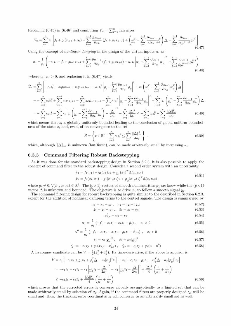
Replacing (6.45) in (6.46) and computing Vn =∑n
i=1 zizi gives
Vn =
n∑
i=1
zi
[
fi + gi(zi+1 + αi)−i−1∑
k=1
∂αi−1
∂xk
(fk + gkxk+1) +
(
ϕT
i−
i−1∑
k=1
∂αi−1
∂xk
ϕT
k
)
∆ −i−1∑
k=1
∂αi−1
∂y(k−1)r
y(k)r
]
(6.47)Using the concept of nonlinear damping in the design of the virtual inputs αi as
αi =1
gi
−cizi − fi − gi−1zi−1 +
i−1∑
k=1
∂αi−1
∂xk
(fk + gkxk+1)− κizi
∣
∣
∣
∣
∣
ϕi−
i−1∑
k=1
∂αi−1
∂xk
ϕk
∣
∣
∣
∣
∣
2
+
i−1∑
k=1
∂αi−1
∂y(k−1)r
y(k)r
)
(6.48)
where ci, κi > 0, and replacing it in (6.47) yields
Vn =n∑
i=1
−ciz2i + zigizi+1 − zigi−1zi−1 − κiz
2i
∣
∣
∣
∣
∣
ϕi−
i−1∑
k=1
∂αi−1
∂xk
ϕk
∣
∣
∣
∣
∣
2
+ zi
(
ϕT
i−
i−1∑
k=1
∂αi−1
∂xk
ϕT
k
)
∆
=−n∑
i=1
ciz2i +
n−1∑
i=1
zigizi+1 −n∑
i=2
zigi−1zi−1 −n∑
i=1
κiz2i
∣
∣
∣
∣
∣
ϕi−
i−1∑
k=1
∂αi−1
∂xk
ϕk
∣
∣
∣
∣
∣
2
+
n∑
i=1
zi
(
ϕT
i−
i−1∑
k=1
∂αi−1
∂xk
ϕT
k
)
∆
=−n∑
i=1
ciz2i −
n∑
i=1
κi
∣
∣
∣
∣
∣
zi
(
ϕi−
i−1∑
k=1
∂αi−1
∂xk
ϕk
)
− ∆
2κi
∣
∣
∣
∣
∣
2
+n∑
i=1
|∆|24κi
≤ −n∑
i=1
ciz2i +
n∑
i=1
‖∆‖2∞
4κi
(6.49)
which means that zi is globally uniformly bounded leading to the conclusion of global uniform bounded-ness of the state xi and, even, of its convergence to the set
S =
x ∈ Rn |
n∑
i=1
ciz2i ≤
n∑
i=1
‖∆‖2∞
4κi
, (6.50)
which, although ‖∆‖∞ is unknown (but finite), can be made arbitrarily small by increasing κi.
6.3.3 Command Filtering Robust Backstepping
As it was done for the standard backstepping design in Section 6.2.3, it is also possible to apply theconcept of command filter to the robust design. Consider a second order system with an uncertainty
x1 = f1(x1) + g1(x1)x2 + ϕ1(x1)
T∆(x, u, t)
x2 = f2(x1, x2) + g2(x1, x2)u+ ϕ2(x1, x2)
T∆(x, u, t)(6.51)
where gi 6= 0, ∀(x1, x2, u) ∈ R3. The (p×1) vectors of smooth nonlinearities ϕ
iare know while the (p×1)
vector ∆ is unknown and bounded. The objective is to drive x1 to follow a smooth signal yr.The command filtering design for robust backstepping is quite similar to the described in Section 6.2.3,
except for the addition of nonlinear damping terms to the control signals. The design is summarized by
z1 = x1 − yr , z2 = x2 − x2,c (6.52)
z1 = z1 − χ1 , z2 = z2 − χ2 (6.53)
x02,c = α1 − χ2 (6.54)
α1 =1
g1(−f1 − c1z1 − s1z1 + yr) , c1 > 0 (6.55)
u0 =
1
g2(−f2 − c2z2 − s2z2 − g1z1 + x2,c) , c2 > 0 (6.56)
s1 = κ1|ϕ1|2 , s2 = κ2|ϕ
2|2 (6.57)
χ1 = −c1χ1 + g1(x2,c − x02,c) , χ2 = −c2χ2 + g2(u− u
0) (6.58)
A Lyapunov candidate can be V = 12 (z
21 + z22). Its time-derivative, if the above is applied, is
V = z1
[
−c1z1 + g1z2 + ϕT
1∆− κ1|ϕ
1|2z1
]
+ z2
[
−c2z2 − g2z1 + ϕT
2∆− κ2|ϕ
2|2z2
]
= −c1z1 − c2z2 − κ1
∣
∣
∣
∣
ϕ1z1 −
∆
2κ1
∣
∣
∣
∣
2
− κ2
∣
∣
∣
∣
ϕ2z2 −
∆
2κ2
∣
∣
∣
∣
2
+|∆|24
(
1
κ1+
1
κ2
)
≤ −c1z1 − c2z2 +‖∆‖2
∞
4
(
1
κ1+
1
κ2
)
(6.59)
which proves that the corrected errors zi converge globally asymptotically to a limited set that can bemade arbitrarily small by selection of κi. Again, if the command filters are properly designed χi will besmall and, thus, the tracking error coordinates zi will converge to an arbitrarily small set as well.
34

Chapter 7
Adaptive Backstepping Design
This chapter introduces a different way of dealing with uncertainties: adaptivity. The backstep-ping design presented in the preceding chapter can acquire such feature in two different ways:directly or indirectly. These two designs are known, respectively, as Integrated Adaptive Back-stepping and Modular Adaptive Backstepping. The modular design is firstly described. This is acertainty equivalence based method, that uses robustness terms and separate on-line estimationof uncertainties. Then, the integrated design is introduced. This design uses tuning functions,defined to satisfy stability conditions, to estimate the uncertainties. The chapter closes with arecently developed integrated design: Immersion and Invariance Adaptive Backstepping.
7.1 Modular Adaptive Backstepping
Differently from the backstepping designs presented so far, the adaptive ones employ a kind of integralnonlinear feedback. This integration lies in the parameter estimation which, in contrast with the staticnonlinear feedback laws previously described, is a type of dynamic feedback.The first adaptive backstepping approach here presented consists in building a robust control law
and estimate the unknown parameter separately. The robustness against estimation errors guaranteesboundedness of the state with respect to the estimation, thus this design is known as Input-to-state StableAdaptive Backstepping.The design process is similar to the one of the robust backstepping described in Section 6.3.2. To
describe the algorithm consider the nth order uncertain system
x1 = f1(x1) + g1(x1)x2 + ϕ1(x1)
T θ(x, u, t)
... (7.1)
xn = fn(x1, . . . , xn) + gn(x1, . . . , xn)u+ ϕn(x1, . . . , xn)
T θ(x, u, t) ,
where u ∈ R, gi(x1, . . . , xi) 6= 0 for any xi ∈ R, i ∈ 1, 2, . . . , n, ϕi(x1, . . . , xi) is a(p × 1) vector of
smooth functions and θ is a (p× 1) vector of unknown functions. The goal is to make the state x1 tracka smooth signal yr.Like in any backstepping design procedure, the first step is to define the error coordinates of the
(tracking) problem zi = xi − αi−1, which have the dynamics
zi =xi − αi−1(x1, . . . , xi, yr, yr, . . . , y(i−1)r , θ)
=fi + gixi+1 + ϕT
iθ −
i−1∑
k=1
∂αi−1
∂xk
(fk + gkxk+1 + ϕT
kθ)−
i−1∑
k=1
∂αi−1
∂y(k−1)r
y(k)r − ∂αi−1
∂θ
˙θ
=fi + gizi+1 + giαi −i−1∑
k=1
∂αi−1
∂xk
(fk + gkxk+1) +
(
ϕT
i−
i−1∑
k=1
∂αi−1
∂xk
ϕT
k
)
θ −i−1∑
k=1
∂αi−1
∂y(k−1)r
y(k)r − ∂αi−1
∂θ
˙θ (7.2)
For simplicity let
wTi = ϕT
i−
i−1∑
k=1
∂αi−1
∂xkϕTk. (7.3)
35

If the control signals αi are defined with both estimated parameters and nonlinear damping terms as
αi =1
gi
[
−cizi − fi − gi−1zi−1 − wTi θ − sizi +
i−1∑
k=1
(
∂αi−1
∂xk
(fk + gkxk+1) +∂αi−1
∂y(k−1)r
y(k)r
)]
(7.4)
where the nonlinear damping term si accounts for the estimation error and estimation update law
si = κi |wi|2+ µi
∣∣∣∣
∂αi−1
∂θ
∣∣∣∣
2
, κi > 0 , µi > 0 (7.5)
If a CLF function is built in the same way as in the robust design procedure as Vi = Vi−1 +12z
2i , the
time-derivative of the of the nth function is
Vn =
n∑
i=1
zizi =
n∑
i=1
[
−ciz2i + ziw
Ti θ − s1z
2i − zi
∂αi−1
∂θ
˙θ
]
=−n∑
i=1
ciz2i −
n∑
i=1
(
κi |wi|2 + µi
∣
∣
∣
∣
∂αi−1
∂θ
∣
∣
∣
∣
2)
z2i +
n∑
i=1
(
wTi θ −
∂αi−1
∂θ
˙θ
)
zi
=−n∑
i=1
ciz2i − κi
n∑
i=1
∣
∣
∣
∣
ziwi −θ
2κi
∣
∣
∣
∣
2
− µi
n∑
i=1
∣
∣
∣
∣
∣
zi∂αi−1
∂θ
T
+˙θ
2µi
∣
∣
∣
∣
∣
2
+1
4
n∑
i=1
(
| ˙θ|2κi
+|θ|2µi
)
≤−n∑
i=1
ciz2i +
1
4
n∑
i=1
(
‖ ˙θ‖2∞
κi
+‖θ‖2
∞
µi
)
(7.6)
which proves the input-to-state stability of zi with respect to θ and˙θ. This property is achieved regardless
of the estimator used, as long as the resulting estimation error and the update law are both bounded.
7.1.1 Nonlinear Extended State Observer
From the survey of estimators done in Section 5.3.2 the Nonlinear Extended State Observer (NESO)appears to be the most suitable for the estimation of unknown time-variable uncertainties. This tendencyis corroborated in (Wang & Gao, 2003), where the NESO proved to have a better performance than aHigh-gain and a Sliding-mode observers in the case of highly variable uncertainty. Furthermore, in (Reale,Ortner, & del Re, 2009) the NESO also outperformed the High-gain observer, the Sliding-mode observerand the Extended Kalman filter in the noise and disturbance rejection control of a combustion enginetest bench simulator including combustion oscillations, noisy measurements and disturbed inputs.The NESO is basically an extended state observer with a nonlinear gain function. The extra state is
used to estimate a specific part of the dynamic model which is not known.Considering again system (7.1), the extended state observer can be written adding n states as
ξi = ϕi(x1, . . . , xi)
T θ(x, u, t) , i ∈ 1, 2, . . . , n (7.7)
resulting in the observer formulation
˙x1 = f1(x1) + g1(x1)x2 + ξ1 − βT
1fal(x, α1, δ1)
˙x2 = f2(x1, x2) + g1(x1, x2)x2 + ξ2 − βT
2fal(x, α2, δ2)
...
˙xn = fn(x1, . . . , xn) + gn(x1, . . . , xn)u+ ξn − βT
nfal(x, αn, δn)
˙ξ1 = −β
T
n+1fal(x, αn+1, δn+1)
˙ξ2 = −β
T
n+2fal(x, αn+2, δn+2)
...
˙ξn = −β
T
2nfal(x, α2n, δ2n)
36

yy = x
y = fal(x)
x1δ
Figure 7.1: Nonlinear gain compared to the linear one for α = 1.
where the estimation gain vectors βihave n entries, all positive. It was assumed that all the states are
measured, thus the estimation error vector x =[x1, . . . , xn
]Tis computed by xi = xi − xi. Furthermore,
fal(x, αi, δi) =
fal(x1, αi, δi)fal(x2, αi, δi)
...fal(xn, αi, δi)
(7.8)
with the function fal being given by (Han, 1995)
fal(xj , αi, δi) =
|xj |αi sign(xj) , |xj | > δi
xj
δ1−αi
i
, |xj | ≤ δi(7.9)
where δi > 0 and 0 < αi ≤ 1. Notice that, for α = 1, (7.9) becomes linear, turning the NESO into anextended state Luenberger observer (fal = x). With this value of α the gains βi can be initially designedby pole placement as a regular linear observer.When the nonlinearities are added the gain function performs as to keep the gain small for large errors
(above δ) and increase it near perfect tracking (below δ) so that the estimator “sticks” to the dynamicsand maintains a small error (see Figure 7.1).The observer, by definition of (7.7), does not use any information from the uncertainty nor from the
regressor function. This feature makes it very versatile, being suitable for a very wide range of disturbedsystems. As for its stability properties, they are derived using the concept of Self-stable Region in (Huang& Han, 2000) for a second order observer.In order to apply the current observer to the modular adaptive backstepping the estimation value and
its time-derivative (the update law) must be bounded. To achieve so one can use the Projection operator,which can impose limits on both quantities forcing the estimation to be bounded. This operator isexplained in Appendix C.2. The update laws are then given by
˙xi = Proj(
fi(xi) + gi(xi)xi+1 + ξi − βT
ifal(x, αi, δi)
)
(7.10)
˙ξi = Proj
(
−βn+i
fal(x, αn+i, δn+i))
(7.11)
7.2 Integrated Adaptive Backstepping
A different approach from the modular design is the integrated design. This method uses the updatelaw as a way to ensure stability of the closed-loop system’s origin. The estimation law is then defined by
37

Lyapunov analysis, which, as it will be seen, does not imply the convergence of the updated parameterto the real value. In fact, that is not a necessary condition for the stability of the closed-loop design.This section begins by presenting the concept of dynamic feedback by tuning functions, being then
extended to higher order systems by recursive design. In both designs the overparametrization is avoided,i.e., the simultaneous multiple estimation of one unknown parameter.
7.2.1 Integrator Backstepping with Tuning Functions
To introduce the design principle behind the integrated adaptive backstepping, we start by consideringthe second order uncertain nonlinear system
x1 = f(x1) + ϕ(x1)T θ + g(x1)x2
x2 = u(7.12)
where (x1, x2, u) ∈ R3 with g(x1) 6= 0, ϕ(x1) a (p×1) vector of smooth nonlinear functions and θ a (p×1)
vector of constant unknown parameters.Having as goal the tracking of a smooth signal yr by the state x1 the design process starts, as the
preceding backstepping methods, by defining the tracking errors z1 = x1 − yr and z2 = x2 − α.The virtual control α should be designed as it was done in Section 6.2.1, i.e., canceling the unstable
nonlinearities. This would yield for the case of known θ
α =1
g(x)
[−c1z1 − f(x)− ϕ(x1)
T θ + yr], c1 > 0 (7.13)
A CLF for the entire system written as V = 12z
21 + 1
2z22 has the time derivative
V = −c1z21 + z1g(x1)z2 + z2
[
u− ∂α
∂x1
(f(x1) + ϕ(x1)
T θ + g(x1)x2
)− ∂α
∂yryr
]
(7.14)
which is positive semi-definite for the input law
u = −c2z2 − g(x1)z1 +∂α
∂x1
(f(x1) + ϕ(x1)
T θ + g(x1)x2
)+
∂α
∂yryr +
∂α
∂yryr , (7.15)
with c2 > 0.Since θ is unknown, the feedback must use an estimate of it: θ. This estimate will have an error
θ = θ − θ which can be accounted for the stability by building the CLF as
V =1
2z21 +
1
2z22 +
1
2θTΓ−1θ , Γ = ΓT > 0 (7.16)
where Γ is the adaptation gain matrix.Taking the time derivative of (7.16) and replacing the true value θ by the estimate θ in (7.13) and in
(7.15) as
α =1
g(x)
[
−c1z1 − f(x)− ϕ(x1)T θ + yr
]
u = −c2z2 − g(x1)z1 +∂α
∂x1
(
f(x1) + ϕ(x1)T θ + g(x1)x2
)
+∂α
∂θ
˙θ +
∂α
∂yryr +
∂α
∂yryr ,
yields
V = −c1z21 − c2z
22 + θ
T(
ϕ(x1)z1 − ϕ(x1)∂α
∂x1z2 − Γ−1 ˙θ
)
(7.17)
where the relation˙θ = − ˙
θ was used.To render (7.17) positive semi-definite the estimate update law can be chosen as
˙θ = Γϕ(x1)
(
z1 −∂α
∂x1z2
)
(7.18)
which replaced in (7.17) results in
V = −c1z21 − c2z
22 ≤ 0 (7.19)
guaranteeing asymptotic tracking of yr by x1.
38

7.2.2 Recursive Design for Higher Order Systems
The procedure described in Section 7.2.1 can be applied recursively to arbitrarily higher order systemsin a parameter strict-feedback system.Consider the following system in the referred form
x1 = f1(x1) + g1(x1)x2 + ϕ1(x1)
T θ
x2 = f2(x1, x2) + g1(x1, x2)x2 + ϕ2(x1, x2)
T θ
...
xn = fn(x1, . . . , xn) + gn(x1, . . . , xn)u+ ϕn(x1, . . . , xn)
T θ ,
(7.20)
where u ∈ R, the function gi(x1, . . . , xi) 6= 0 for any (x1, . . . , xn) ∈ Rn, ϕ
i(x1, . . . , xi) is a (p× 1) vector
of known smooth nonlinearities and θ is a (p× 1) vector of constant unknown parameters.The control goal is to make x1 track a smooth signal yr. The error variables zi = xi − αi−1, with
α0.= yr for i ∈ 1, 2, . . . , n, have the dynamics
zi = xi − αi−1(x1, . . . , xi−1, yr, yr, . . . , y(i−1)r , θ)
= fi + gixi+1 + ϕTiθ −
i−1∑
k=1
∂αi−1
∂xk(fk + gkxk+1 + ϕT
kθ)−
i−1∑
k=1
∂αi−1
∂y(k−1)r
y(k)r − ∂αi−1
∂θ
˙θ
where α0.= yr and xn+1 = αn
.= u.
As done in (7.16) a CLF can be written that accounts for the parameter estimation error as
Vi =1
2
i∑
k=1
z2k +1
2θTΓ−1θ , Γ = ΓT > 0 (7.21)
which has the time derivative
Vi =i∑
k=1
zkzk + θTΓ−1 ˙θ (7.22)
The time derivative of Vi for i = n is
Vn =n∑
i=1
zizi + θTΓ−1 ˙θ
=
n∑
i=1
[
zifi + zigizi+1 + zigiαi + ziϕTiθ − zi
i−1∑
k=1
∂αi−1
∂xk(fk + gkxk+1 + ϕT
kθ)
−zi
i−1∑
k=1
∂αi−1
∂y(k−1)r
y(k)r − zi∂αi−1
∂θ
˙θ
]
− θTΓ−1 ˙θ
(7.23)
where zn+1 = 0.The stabilizing control signals αi can be defined as
αi =1
gi
(
−cizi − fi − gi−1zi−1 − ϕTiθ +
i−1∑
k=1
∂αi−1
∂xk(fk + gkxk+1 + ϕT
kθ) +
i−1∑
k=1
∂αi−1
∂y(k−1)r
y(k)r +∂αi−1
∂θ
˙θ
)
(7.24)with ci > 0 and g0z0 = 0.Applying (7.24) to (7.23) gives
Vn =
n∑
i=1
[
−ciz2i + zigizi+1 − zigi−1zi−1 + ziϕ
T
iθ − zi
i−1∑
k=1
∂αi−1
∂xk
ϕT
kθ
]
− θTΓ−1 ˙
θ
=−n∑
i=1
ciz2i + θ
Tn∑
i=1
ϕizi − θ
Tn∑
i=1
(
i−1∑
k=1
∂αi−1
∂xk
ϕk
)
zi − θTΓ−1 ˙
θ
=−n∑
i=1
ciz2i + θ
T
[
n∑
i=1
(
ϕi−
i−1∑
k=1
∂αi−1
∂xk
ϕk
)
zi − Γ−1 ˙θ
]
(7.25)
39

It is easy to see that for (7.25) to be negative definite the update law can be chosen as
˙θ = Γ
n∑
i=1
(
ϕi−
i−1∑
k=1
∂αi−1
∂xkϕk
)
zi (7.26)
and to verify it, (7.26) shall be applied to (7.25) yielding
Vn = −n∑
i=1
ciz2i ≤ 0 (7.27)
which proves the global asymptotic tracking of yr by x1. It is also guaranteed the convergence of theparameter estimation, although not necessarily to the true value θ.
7.2.3 Design for Time-varying Uncertainties
The integrated design methodology presented so far can only be used for systems with constant un-certainties. However, it can be extended to systems with time-varying uncertainties using addition ofrobustness terms. This design is nothing more than a modular adaptive backstepping law with a tunningfunction estimator. Such method was introduced in (Ge & Wang, 2002) for state feedback control andlater in (Zhou & Wen, 2008) for output feedback laws. Here, only the state feedback design will bedescribed.Consider a system similar to (7.20) but where the θ is non-constant
x1 = f1(x1) + g1(x1)x2 + ϕ1(x1)
T θ(x, u, t)
x2 = f2(x1, x2) + g1(x1, x2)x2 + ϕ2(x1, x2)
T θ(x, u, t)
...
xn = fn(x1, . . . , xn) + gn(x1, . . . , xn)u+ ϕn(x1, . . . , xn)
T θ(x, u, t) ,
(7.28)
where u ∈ R, the control gain function gi(x1, . . . , xi) 6= 0 for any xi ∈ R, i ∈ 1, 2, . . . , n, ϕi(x1, . . . , xi)
is a(p× 1) vector of smooth nonlinearities and θ is a (p× 1) vector of unknown functions.The robustness-added virtual inputs αi are given exactly as (7.4) by
αi =1
gi
−cizi − fi − gi−1zi−1 −(
ϕi−
i−1∑
k=1
∂αi−1
∂xkϕk
)T
θ − sizi
+
i−1∑
k=1
∂αi−1
∂xk(fk + gkxk+1) +
i−1∑
k=1
∂αi−1
∂y(k−1)r
y(k)r
] (7.29)
where the nonlinear damping terms si are written
si = κi
∣∣∣∣∣ϕi−
i−1∑
k=1
∂αi−1
∂xkϕk
∣∣∣∣∣
2
+ µi
∣∣∣∣
∂αi−1
∂θ
∣∣∣∣
2
, κi > 0 , µi > 0 (7.30)
To the estimation update law in (7.26) the projection operator was applied yielding
˙θ = Proj
(
Γn∑
i=1
[
ϕi−
i−1∑
k=1
∂αi−1
∂xkϕk
]
zi
)
(7.31)
The projection operator uses predefined limits to ensure the boundedness of both the estimated param-eter and its time-derivative. This operator is further explained in Appendix C.2.If a Lyapunov function is defined as V =
∑ni=1 z
2i , its time-derivative along the trajectories of the
closed-loop system with feedback laws (7.29) will, as in (7.6), result in
V ≤ −n∑
i=1
ciz2i +
1
4
n∑
i=1
(
‖ ˙θ‖2∞κi
+‖θ‖2∞µi
)
(7.32)
which, provided that the projection algorithm is used, proves the input-to-state stability of zi with respectto the estimation.
40

7.2.4 Proof of Estimation Convergence for Disturbed Systems
Although when using the integrated adaptive backstepping design method the estimation convergenceto the true value of the uncertain parameter is not guaranteed, here a special case is presented in whichthe true parameter value is indeed identified. This proof considers only the systems with added andmatched disturbance, i.e, with constant regressor function. Both constant and time-varying disturbanceswill be considered.Consider a scalar system in the referred form
x = f(x) + g(x)u+ d , (7.33)
where (x, u, d) ∈ R3, d is unknown and g(x) 6= 0, ∀x. The control goal is the same as in the previous
descriptions: make the state x track a smooth reference yr.
Constant Disturbance
Let d be a constant value. Applying the integrated adaptive backstepping method gives the controlinput and estimation update law
u =1
g(x)
(
−f(x)− cz − d+ yr
)
, c > 0 (7.34)
˙d = γz , γ > 0 (7.35)
where z = x− yr is the error coordinate.The tracking and estimation error dynamics in closed-loop system becomes
[
z˙d
]
=
[−c 1−γ 0
] [z
d
]
(7.36)
where d = d− d and˙d = − ˙
d.Since both the control gain c and the estimation gain γ are positive the error system matrix (7.36) is
Hurwitz, which means that both z and d have an asymptotically stable equilibrium at the origin
limt→∞
(x, d) = (yr, d) (7.37)
Time-variable Disturbance
If d(t) is now a function of time, the integrated algorithm has to be modified as described in Section 7.2.3,i.e. a robustness term has to be added to the control input signal (7.34) as
u =1
g(x)
(
−f(x)− cz − d− sz + yr
)
, c > 0 , s = κ > 0 (7.38)
Having now˙d = d− ˙
d, the error dynamics system becomes
[
z˙d
]
=
[−c− κ 1−γ 0
] [z
d
]
+
[01
]
d (7.39)
If the nonlinear damping gain and the estimation gain are given by κ = k1/ε and γ = k2/ε2 the transfer
function from d to the states of (7.39) can be written as
G(s) =ε
(εs)2 + s(ε2c+ εk1) + k2
[ε
εs+ εc+ k1
]
(7.40)
It is easy to verify that limε→0 G(s) = 0, meaning that for high robustness and estimation gains thesystem is able to both track the reference signal and estimate correctly the disturbance.
41

7.3 Command Filtering Adaptive Backstepping
In Section 6.2.3 the introduction of command filters in the backstepping design made it unnecessary tocompute the derivatives of the virtual control signals. In the framework of adaptive backstepping this canalso be very useful, especially in the integrated design, where the estimation update law depends on thesuccessive derivatives of αi. In this section the command filtering design for robustness-added integratedadaptive and modular adaptive backstepping designs will be described. As both use nonlinear dampingterms, their filtered design is similar to the one presented for the robust backstepping. The commandfiltered adaptive backstepping with tuning functions is described in (Yip & Hedrick, 1998) where it isreferred to as Adaptive Dynamic Surface Control. In (Farrell, Polycarpou, & Sharma, 2005) the sameconcept is applied to design an adaptive flight control law. Magnitude and rate constraints can be alsoadded to the controller as it is shown in (Farrell, Polycarpou, & Sharma, 2003). A design with nonlineardamping terms is used in (Zhang & Lin, 2010).Consider a second order nonlinear system
x1 = f1(x) + g1(x)x2 + ϕ1(x)T θ(x, u, t)
x2 = f2(x) + g2(x)u+ ϕ2(x)T θ(x, u, t)
(7.41)
where gi(x) 6= 0, ∀x ∈ R2. Additionally, ϕ
i(x) are (p × 1) vectors of known and smooth nonlinearities,
while θ(x, u, t) is an unknown (p× 1) vector of bounded nonlinear functions. Let the control task be thetracking of a smooth signal yr by the state x1.The first step is, as it became usual, the definition of the error coordinates
z1 = x1 − yr , z2 = x2 − x2,c (7.42)
Let the virtual control α be given by
α1 =1
g1
(
−f1 − c1z1 − s1z1 − ϕT1θ + yr
)
, c1 > 0 (7.43)
where z1 will be defined later on in the design. The nonlinear damping term s1 is
s1 = κ1|ϕ1|2 , κ1 > 0 (7.44)
The signal α1 is corrected to produce x02,c by
x02,c = α1 − χ2 (7.45)
This signal is the raw virtual control, which is then filtered to obtain x2,c and its time-derivative x2,c.In this process limits may be introduced in terms of magnitude and rate. The filter effect in the errorcoordinate z1 can be estimated by
χ1 = −c1χ1 + g1(x2,c − x02,c) (7.46)
The following error coordinates are introduced to remove the filtering effect
z1 = z1 − χ1 , z2 = z2 − χ2 (7.47)
Define the Lyapunov candidate V1 = 12 z
21 . Its time-derivative is given by
V1 = z1
[
f1 + g1x2 + ϕT1θ − yr − χ1
]
= z1
[
f1 + g1(z2 + x2,c − x02,c) + g1(α1 − χ2) + ϕT
1θ − yr − χ1
]
= z1
[
−c1z1 + g1(z2 + x2,c − x02,c)− g1χ2 − s1z1 + ϕT
1θ − χ1
]
= z1
[
−c1z1 + g1z2 + g1(x2,c − x02,c)− s1z1 + ϕT
1θ + c1χ1 − g1(x2,c − x0
2,c)]
= −c1z21 + z1g1z2 − s1z
21 + z1ϕ
T1θ
(7.48)
The raw control signal u0 is given by
u0 =1
g2
(
−f2 − c2z2 − g1z1 − s2z2 − ϕT2θ + x2,c
)
, s2 = κ2|ϕ2|2 (7.49)
42

with c2 > 0 and κ2 > 0.The raw signal u0 is, again, filtered to produce u and u. The effect of this filtering process on z2 is
estimated byχ2 = −c2χ2 + g2(u− u0) . (7.50)
A second Lyapunov function may be defined based on V1 as V2 = V1 + 12 z
22 . This function has the
time-derivative
V2 = V1 + z2
[
f2 + g2(u− u0) + g2u0 + ϕT
2θ − x2,c − χ2
]
= −c1z21 + z1g1z2 − s1z
21 + z1ϕ
T1θ + z2
[
−c2z2 − g1z1 − s2z2 + ϕT2θ]
= −c1z21 − c2z
22 − κ1|ϕ1
|2z21 − κ2|ϕ2|2z22 + z1ϕ
T1θ + z2ϕ
T2θ
= −c1z1 − c2c2 − κ1
∣∣∣∣∣z1ϕ1
+θ
2κ1
∣∣∣∣∣
2
+θ2
4κ1− κ2
∣∣∣∣∣z2ϕ2
+θ
2κ2
∣∣∣∣∣
2
+θ2
4κ2
≤ −c1z1 − c2c2 +‖θ‖2∞4
(1
κ1+
1
κ2
)
(7.51)
which proves the global asymptotic stability of the compensated error zi outside a compact ball aroundthe origin. If the filters are tunned properly, χi will be small and the effect of the filters will be negligible.Hence, the original error coordinates zi will have the same stability properties as zi. The proof of thisstatement uses singular perturbation theory and can be found in (Yip & Hedrick, 1998).The set to which zi converge can be made as small as desired by increasing all κi, as long as the
estimation error θ is bounded. This boundedness is achieved, once again, by the usage of the projectionoperator. In the modular design the estimation law is the described in Section 7.1.1. For the integrateddesign the law (7.31) is simplified by the introduction of command filters becoming
˙θ = Proj
(
Γ
n∑
i=1
ϕizi
)
(7.52)
7.4 Immersion and Invariance Adaptive Backstepping
In this section the recently developed adaptive backstepping control design by Immersion and Invariance(I&I) is introduced. This method uses the definition of an invariant manifold to ensure that all thesolutions staying in its surface converge to the equilibrium state. To achieve so, this theory uses theclosed-loop target dynamics to properly design an estimation law for the adaptive control. The mainliterature on this theory is the book (Astolfi, Karagiannis, & Ortega, 2008).The present section begins by defining the basic concepts behind Immersion and Invariance control
theory. Then the uncertainty observer design is described, followed by the design methodology of thecontroller.The design described in this thesis focus on state feedback laws only, the extension to output feedback
systems is possible as presented in (Karagiannis, Astolfi, & Ortega, 2002; Karagiannis, Jiang, Ortega, &Astolfi, 2004; Karagiannis, Carnevale, & Astolfi, 2007).
7.4.1 Concept of Immersion and Invariance
The Immersion and Invariance control design was first introduced in (Astolfi & Ortega, 2001). Itsname comes from the fact that the design method uses an immersion of the system into the desireddynamics together with the definition of an invariant manifold. To illustrate this principle consider thenonlinear system
x = f(x) + g(x)u , (7.53)
where u ∈ Rm and for x ∈ R
n, g(x) 6= 0. The control objective is to find a law u = v(x) that globallyasymptotically stabilizes the origin. To do so, we first find a target dynamical system
ξ = α(x) , (7.54)
with ξ ∈ Rp, p < n, which is globally asymptotically stable at the origin and has a smooth mapping
x = π(ξ) and a control law such that
π(ξ(0)) = x(0) , (7.55)
π(0) = 0 , (7.56)
43

and
f(π(ξ)) + g(π(ξ))v(π(ξ)) =∂π
∂ξα(ξ) (7.57)
If these conditions are verified, all the trajectories x(t) of the closed-loop system
x = f(x) + g(x)v(x) (7.58)
are images through the mapping π(·) of trajectories ξ(t) of the target system. Having in mind that thetarget dynamics α(x) has an asymptotically stable origin and from (7.56), the trajectories x(t) mustconverge to the origin. This means that to effectively stabilize the system (7.53), the differential equation(7.57) must be solved with initial conditions (7.55) and (7.56).The discussed general theory can be applied to design adaptive control laws for nonlinear systems with
parametric uncertainties. To illustrate the design method consider once again system (7.53), where thefunctions f(x) and g(x) may depend on a vector of uncertain parameters θ ∈ R
q. The adaptive controlproblem is then to find a law
u = v(x, θ) ,˙θ = w(x, θ) (7.59)
such that all the closed-loop trajectories are bounded and asymptotically converge to the equilibriumstate. To do so it is assumed that there is a full-information control law such that the closed-loop systemhas a globally asymptotically stable equilibrium state xe.
Definition 7.1. (adaptive I&I stabilizability)(Astolfi et al., 2008) The system (7.53) is said to beadaptively I&I stabilizable if there exist β(·) and w(·) such that all trajectories of the extended system
x =f(x) + g(x)v(x, θ + β(x)) ,
˙θ =w(x, θ)
are bounded and satisfy
limt→∞
[
g(x(t))v(x(t), θ + β(x(t)))− g(x(t))v(x(t), θ)]
= 0 (7.60)
Condition (7.60) is satisfied by all trajectories x(t) staying on the manifold
M =
(x, θ) ∈ Rn × R
q | θ − θ + β(x) = 0
(7.61)
Additionally, Definition 7.1, together with the existence of a full-information control law v(x, θ) thatrenders xe globally asymptotically stable, implies that all trajectories x(t) of the closed-loop adaptivelyI&I controlled asymptotically converge to xe.It should be noted that the controller developed by I&I method does not follow the certainty equiva-
lence philosophy, in the sense that the parameter estimate is not applied directly to the full-informationfeedback law. Instead, the true parameter θ is replaced by θ + β(x), where the function β(x) adds a
“proportional” action to the “integral” action of the estimate update law˙θ. For so, this kind of adaptive
scheme is also known as nonlinear PI adaptation.One must finally highlight that, because the functions f(x) and g(x) may both depend on the uncertain
parameter θ, it is not guaranteed that the estimate θ converges, but only that it remains bounded. Inmany cases, though, it is indeed possible to establish an equilibrium (x, θ) = (xe, θ) that is globallyasymptotically stable. Such a case is described in example 7.1.
Example 7.1. (I&I adaptive control design)Consider the scalar nonlinear system
x = x+ θex + u (7.62)
where x ∈ R is the state, u ∈ R is the control input and θ ∈ R is a constant unknown parameter. If thevalue of θ was known the feedback
u = −cx− θex , c > 1 (7.63)
would asymptotically stabilize the equilibrium x = 0. As this is not the case, an estimated value mustbe used instead.The earlier described Lyapunov method sugests the definition of a control Lyapunov function such as
V =1
2x2 +
(θ − θ)2
2γ. (7.64)
44

Defining the estimation update law as
˙θ = γxex , γ > 0 . (7.65)
renders the time-derivative of V negative semi-definite
V = −cx2 (7.66)
which proves global stability and convergence of x to zero.The I&I approach, on the other hand, starts by the definition of a one-dimensional manifold as
M =
(x, θ) ∈ R2 | θ − θ + β(x) = 0
(7.67)
where β(x) is a continuous function that will be selected later on. To render the manifold M invariantwe define a off-the-manifold coordinate
η = θ − θ + β(x) (7.68)
which has to be made globally stable at the origin.The system (7.62) can be restricted to the invariant manifold M by writing
x = x+ (θ + β(x))ex + u (7.69)
which means that the feedback
u = −cx+ (θ + β(x))ex , c > 1 (7.70)
completely linearizes the restricted system.The dynamics of the off-the-manifold coordinate can be given by
η =˙θ +
∂β(x)
∂x
(
x+ (θ + β(x)− η)ex + u)
=˙θ +
∂β(x)
∂x(−(c− 1)x− ηex) . (7.71)
Defining the update law as˙θ =
∂β(x)
∂x(c− 1)x (7.72)
yields
η = −∂β(x)
∂xexη . (7.73)
Let a Lyapunov function for η be written
V =η2
2γ. (7.74)
Its time-derivative along the trajectories of (7.73) is
V = − 1
γ
∂β(x)
∂xexη2 (7.75)
which can be rendered negative semi-definite by an appropriate selection of β(x). A possible choice is,for example,
β(x) = γx . (7.76)
The resulting closed-loop system becames a cascade interconnection of two stable systems
x = −(c− 1)x− exη
η = −γexη(7.77)
which can be tuned by defining c and γ. The interconnection makes this design much easier to tune,being the performance of the two subsystems improved via the increase of any of the two gains. Such didnot happen for the tuning function design, where a higher γ does not imply a better regulation behavior.Figure 7.2 compares the responses of the two derived adaptive controllers for γ = 1, c = 2, θ = 3 and
(x0, θ0) = (1, 0). As can be seen, the two controllers drive the system state to zero, although with visiblydifferent performances. The estimated parameters from both designs converge to the true value θ = 3,which is due to the nonzero value of the regressor function ex at the origin.
45

I&ITuning Function
θ
Time [s]
ux
0 5 10 15
0 5 10 15
0 5 10 15
0
1
2
3
4
5
6
−60
−40
−20
0
−2
0
2
4
Figure 7.2: State regulation, control effort and parameter estimation evolutions of the tuning functionadaptive controller and the I&I adaptive design.
7.4.2 Design for Higher Order Systems
The principles introduced in the previous section can be synthesized for the adaptive controller designfor nth order parametric strict-feedback systems. This design was adapted from a less general designintroduced in (Karagiannis & Astolfi, 2008). Consider the following system in the referred form
x1 = f1(x1) + g1(x1)x2 + ϕ1(x1)
T θ
...
xn = fn(x1, . . . , xn) + gn(x1, . . . , xn)u+ ϕn(x1, . . . , xn)
T θ ,
(7.78)
where u ∈ R, the function gi(x1, . . . , xi) 6= 0 for any (x1, . . . , xn) ∈ Rn, ϕ
i(x1, . . . , xi) is a (p× 1) vector
of known smooth nonlinearities and θ is a (p × 1) vector of constant unknown parameters. The controlgoal is to make x1 asymptotically track a smooth reference yr.
Estimator Design
The first step is the design of an overparameterized observer of order np. For this define the off-the-manifold (error) coordinates
ηi= θi − θ + βi(x1, . . . , xi) , i ∈ 1, 2, . . . , n (7.79)
where the estimates θi are the estimator states and βi are smooth functions that will be defined later on.The error dynamics are given by
ηi=
˙θi +
i∑
k=1
∂βi
∂xk
(
fk + gkxk+1 + ϕTkθ)
=˙θi +
i∑
k=1
∂βi
∂xk
(
fk + gkxk+1 + ϕTk
(
θi + βi − ηi
))
(7.80)
46
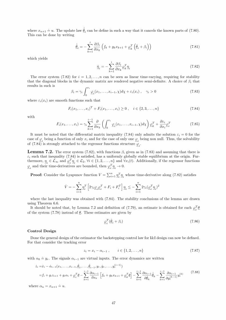
where xn+1.= u. The update law
˙θi can be define in such a way that it cancels the known parts of (7.80).
This can be done by writing
˙θi = −
i∑
k=1
∂βi
∂xk
(
fk + gkxk+1 + ϕTk
(
θi + βi
))
(7.81)
which yields
ηi= −
i∑
k=1
∂βi
∂xkϕTkηi
(7.82)
The error system (7.82) for i = 1, 2, . . . , n can be seen as linear time-varying, requiring for stabilitythat the diagonal blocks in the dynamic matrix are rendered negative semi-definite. A choice of βi thatresults in such is
βi = γi
∫ xi
0
ϕi(x1, . . . , xi−1, χ)dχ+ εi(xi) , γi > 0 (7.83)
where εi(xi) are smooth functions such that
Fi(x1, . . . , xi)T + Fi(x1, . . . , xi) ≥ 0 , i ∈ 2, 3, . . . , n (7.84)
with
Fi(x1, . . . , xi) = γi
i−1∑
k=1
∂
∂xk
(∫ xi
0
ϕi(x1, . . . , xi−1, χ)dχ
)
ϕTk+
∂εi∂xi
ϕTi
(7.85)
It must be noted that the differential matrix inequality (7.84) only admits the solution εi = 0 for thecase of ϕ
ibeing a function of only xi and for the case of only one ϕ
ibeing non null. Thus, the solvability
of (7.84) is strongly attached to the regressor functions structure ϕi.
Lemma 7.2. The error system (7.82), with functions βi given as in (7.83) and assuming that there isεi such that inequality (7.84) is satisfied, has a uniformly globally stable equilibrium at the origin. Fur-thermore, η
i∈ L∞ and ϕT
iηi∈ L2, ∀i ∈ 1, 2, . . . , n and ∀xi(t). Additionally, if the regressor functions
ϕiand their time-derivatives are bounded, then ϕT
iηi→ 0.
Proof: Consider the Lyapunov function V =∑n
i=1 ηTiηiwhose time-derivative along (7.82) satisfies
V =−n∑
i=1
ηTi
[
2γiϕiϕTi+ Fi + FT
i
]
ηi≤ −
n∑
i=1
2γi(ϕTiηi)2
where the last inequality was obtained with (7.84). The stability conclusions of the lemma are drawnusing Theorem 6.6.It should be noted that, by Lemma 7.2 and definition of (7.79), an estimate is obtained for each ϕT
iθ
of the system (7.78) instead of θ. These estimates are given by
ϕTi(θi + βi) (7.86)
Control Design
Done the general design of the estimator the backstepping control law for I&I design can now be defined.For that consider the tracking error
zi = xi − αi−1 , i ∈ 1, 2, . . . , n (7.87)
with α0.= yr. The signals αi−1 are virtual inputs. The error dynamics are written
zi =xi − αi−1(x1, . . . , xi−1, θ1, . . . , θi−1, yr, yr, . . . , y(i−1)r )
=fi + gizi+1 + giαi + ϕT
iθ −
i−1∑
k=1
∂αi−1
∂xk
[
fk + gkxk+1 + ϕT
kθ]
−i−1∑
k=1
∂αi−1
∂θk
˙θk −
i−1∑
k=1
∂αi−1
∂y(k−1)r
y(k)r
(7.88)
where αn = xn+1.= u.
47

Using the estimates from the design of the previous section the virtual controls αi can be defined as
αi =1
gi
[
−κi − fi − ϕT
i(θ + βi) +
i−1∑
k=1
∂αi−1
∂xk
(
fk + gkxk+1 + ϕT
k(θk + βk)
)
+
i−1∑
k=1
∂αi−1
∂θk
˙θk +
i−1∑
k=1
∂αi−1
∂y(k−1)r
y(k)r
]
(7.89)
where κi is a function yet to be defined.The feedback laws (7.89) cause the error dynamics (7.88) to become
zi = −κi + gizz+1 − ϕTiηi+
i−1∑
k=1
∂αi−1
∂xkϕTkηk
(7.90)
Consider the Lyapunov function for the integrated control and estimation laws
Vn =n∑
i=1
ηT η +n∑
i=1
z2i (7.91)
To attain a stable equilibrium, the time-derivative of (7.91) has to be rendered negative (semi-)definiteby design of the feedback function κi.Taking the derivative of (7.91) along the trajectories of (7.90) and using Lemma 7.2 yields
Vn =
n∑
i=1
2ηTη +
n∑
i=1
2zizi ≤ −n∑
i=1
2γi(ϕT
iηi)2 +
n∑
i=1
2
[
−ziκi + zigizz+1 − ziϕT
iηi+ zi
i−1∑
k=1
∂αi−1
∂xk
ϕT
kηk
]
≤−n∑
i=1
2γi(ϕT
iηi)2 +
n∑
i=1
2 [−ziκi + zigizz+1] +n∑
i=1
[
−(
zi√ε+
ϕT
iηi√
ε
)2
+ εz2i +
(ϕT
iηi)2
ε
]
+
n∑
i=1
[
εz2i
i−1∑
k=1
(
∂αi−1
∂xk
)2
+1
ε
i−1∑
k=1
(ϕT
kηk)2 −
i−1∑
k=1
(
zi√ε∂αi−1
∂xk
−ϕT
kηk√ε
)2]
≤−n∑
i=1
[
2γi −1
ε(n− i+ 1)
]
(ϕT
iηi)2 +
n∑
i=1
2 [−ziκi + zigizz+1] +n∑
i=1
εz2i +
n∑
i=1
[
εz2i
i−1∑
k=1
(
∂αi−1
∂xk
)2]
(7.92)
where ε > 0 is constant. The rearranging was performed by squares completion. Some stable quadraticterms were neglected during the simplification.It is easy to see that the function κi defined as
κi = −cizi −ε
2zi − gi−1zi−1 − zi
ε
2
i−1∑
k=1
(∂αi−1
∂xk
)2
, ci > 0 (7.93)
renders (7.92) negative (semi-)definite for
γi ≥1
2ε(n− i+ 1) (7.94)
To prove so, one may replace (7.93) in (7.92) resulting in
Vn ≤ −2
n∑
i=1
ciz2i −
n∑
i=1
[
2γi −1
ε(n− i+ 1)
]
(ϕTiηi)2 (7.95)
which if (7.94) holds gives
Vn ≤ −2
n∑
i=1
ciz2i ≤ 0 (7.96)
that by Theorem 6.6 assures global convergence of both zi and ϕTiηito zero, which guarantees global
tracking of yr by the state x1. This result, as explained, depends on the fulfilling of condition (7.94) andon the existence of εi such that (7.84) is satisfied.
48

7.4.3 Time-varying Uncertainties
The algorithm described so far has unique stability properties in the case of constant uncertain param-eters. In this section it will be proved that, for a special class of systems with scalar regressor functions,the I&I design provides input-to-state stability property to the adaptively controlled system.Consider a system similar to (7.78) but where each state function is affected by a different scalar
time-varying uncertainty, such as
x1 = f1(x1) + g1(x1)x2 + ϕ1(x1)θ1(x, u, t)
...
xn = fn(x1, . . . , xn) + gn(x1, . . . , xn)u+ ϕn(x1, . . . , xn)θn(x, u, t) ,
(7.97)
where u ∈ R and gi(x1, . . . , xi) 6= 0, ∀(x1, . . . , xn) ∈ Rn. The regressor functions ϕi(x1, . . . , xi) and the
uncertainties θi(x, u, t) are both scalar and smooth.Defining the off-the-manifold coordinate as in (7.79), its time-derivative is now given by
ηi =˙θi − θi +
i∑
k=1
∂βi
∂xkxk (7.98)
which, maintaining a similar update law as in (7.81), yields
ηi = −θi −i∑
k=1
∂βi
∂xkϕkηi (7.99)
If βi is chosen in a similar manner as in (7.83) with εi satisfying condition (7.57), then the time-derivativeof a Lyapunov function W =
∑ni=1 η
2i along the trajectories of (7.99) is given by
W =−n∑
i=1
2ηiθi −n∑
i=1
(
2ηi
i∑
k=1
∂βi
∂xkϕkηi
)
≤ −n∑
i=1
2ηiθi −n∑
i=1
2γi(ϕiηi)2 (7.100)
where the inequality was obtained by application of Lemma 7.2.Let the following conditions hold for all regressor functions ϕi:
ϕi 6= 0 , |ϕ−1i | ≤ ρi , ρi > 0 , ∀(x1, . . . , xi) ∈ R
i (7.101)
for a set of positive constants ρi. Then (7.100) can be simplified as
W ≤−n∑
i=1
2(
ηiθi + γi(ϕiηi)2)
≤ −n∑
i=1
γi(ϕiηi)2 −
n∑
i=1
γi
(
ϕiηi +θi
γiϕi
)2
+
n∑
i=1
θ2iγiϕ2
i
(7.102)
≤−n∑
i=1
γi(ϕiηi)2 +
n∑
i=1
θ2iγiϕ2
i
(7.103)
If a control law is designed as done in (7.89) and (7.93), the time-derivative of the Lyapunov functionV = W +
∑ni=1 z
2i will be
V ≤− 2
n∑
i=1
ciz2i −
n∑
i=1
[
γi −1
ε(n− i+ 1)
]
(ϕiηi)2 +
n∑
i=1
θ2iγiϕ2
i
≤ −2
n∑
i=1
ciz2i +
n∑
i=1
ρ2iγi
‖θi‖2∞ (7.104)
where the last inequality holds for
γi ≥1
ε(n− i+ 1) (7.105)
In the presence of smooth uncertainties (continuously differentiable with bounded derivatives), if theregressor functions are such that the conditions (7.101) are satisfied, the gains γi are designed so that(7.105) is true and also if the there is εi such that (7.84) is fulfilled, then (7.104) proves the input-to-state
stability of zi with respect to θ. This means that by increasing the gain γi the compact set around theorigin to which the trajectories zi(t) of the closed-loop system converge can be made arbitrarily small.It should be noted that condition (7.101) is very stringent on the regressor functions. However, it holds
for any constant scalar regressor, i.e., for the problem of additive disturbance estimation and rejection.
49

7.4.4 Command Filtered I&I Control Design
In this section the command filtering method is applied to the Immersion and Invariance design, reducingthe derivation burden and allowing the introduction of magnitude and rate limits. The design process ispartially adapted from (Sonneveldt, 2010) and is here described for system (7.78). It starts, as usual, bydefining the error coordinates zi = xi−xi,c with i ∈ 1, 2, . . . , n. The signals xi,c will be defined furtherahead in the design. The compensated error coordinates are
zi = zi − χi (7.106)
where χi will be defined later on. The dynamics of the compensated errors are given by
˙zi = zi − χi = fi + gixi+1 + ϕTiθ − xi,c − χi (7.107)
where xn+1.= u. Let the raw control signals be defined as
x0i+1,c =
1
gi
(
−fi − cizi − gi−1zi−1 − ϕTi(θi + βi) + xi,c
)
− χi+1 , i ∈ 1, 2, . . . , n− 1
u0 =1
gn
(
−fn − cnzn − gn−1zn−1 − ϕTn(θn + βn) + xn,c
) (7.108)
with ci > 0, cn > 0, x1,c.= yr, z0 = 0 and g0 = 0. These signals are filtered to produce xi+1,c and u and
their derivatives xi+1,c and u. The effect of the filter on the error coordinates is estimated by
χi = −ciχi + gi(xi,c − x0i,c) , i ∈ 1, 2, . . . , n− 1
χn = −cnχn + gn(u− u0)(7.109)
Define the Lyapunov function V =∑n
i=1(z2i + ηT
iηi). Its time-derivative along the trajectories of ˙zi is
V =n∑
i=1
2zi(
fi + gixi+1 + ϕT
iθ − xi,c − χi
)
+n∑
i=1
2ηT
iηi
=n∑
i=1
2zi(
fi + gi(zi+1 + xi+1,c − x0i+1,c) + gix
0i+1,c + ϕ
T
iθ − xi,c − χi
)
+n∑
i=1
2ηT
iηi
=n∑
i=1
2zi(
−cizi + gi(zi+1 + xi+1,c − x0i+1,c)− ϕ
T
iηi− giχi+1 − gi−1zi−1 − χi
)
+n∑
i=1
2ηT
iηi
=n∑
i=1
2zi(
−cizi + gizi+1 − gi−1zi−1 − ϕT
iηi
)
+n∑
i=1
2ηT
iηi
= −n∑
i=1
2ciz2i −
n∑
i=1
2ziϕT
iηi+
n∑
i=1
2ηT
iηi
to which the result of Lemma 7.2 can be applied yielding
V ≤ −n∑
i=1
2ciz2i −
n∑
i=1
2ziϕT
iηi−
n∑
i=1
2γi(ϕT
iηi)2
= −n∑
i=1
(2ci − ε) z2i −n∑
i=1
(
ϕT
iηi√
ε+
√εzi
)2
−n∑
i=1
(
2γi −1
ε
)
(ϕT
iηi)2
≤−n∑
i=1
(2ci − ε) z2i −n∑
i=1
(
2γi −1
ε
)
(ϕT
iηi)2 (7.110)
where ε > 0. Let
ci = ci −ε
2, ci > 0 and γi ≥
1
2ε(7.111)
then (7.110) becomes
V ≤ −n∑
i=1
2ciz2i ≤ 0 (7.112)
proving the global stability of the origin of the compensated tracking errors. Again, if the commandfilters are designed with a high enough bandwidth the compensation signals χi will be small, having anegligible effect on the closed-loop system. Hence, the stability properties of zi can, in that case, beextended to the real tracking errors zi, rendering global tracking of the reference signal.It should be noted that the result of Section 7.4.3 for time-varying uncertainties can be easily extended
to the command filtered design for the same system yielding the same input-to-state stability properties.
50
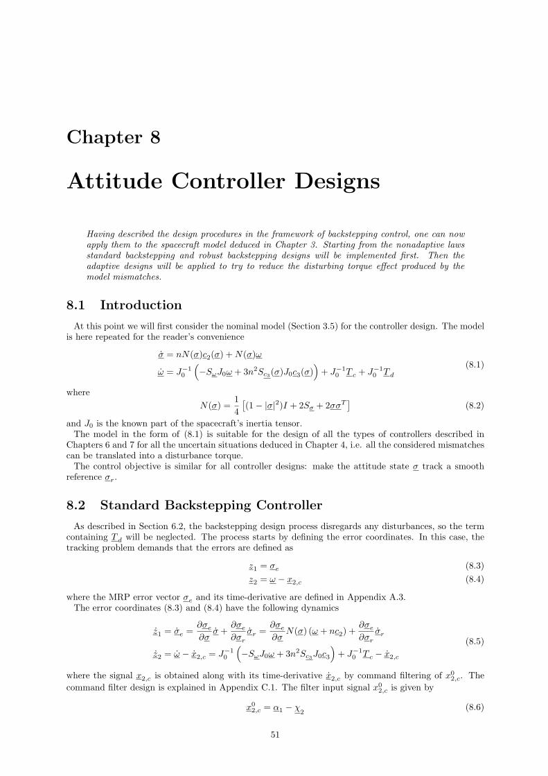
Chapter 8
Attitude Controller Designs
Having described the design procedures in the framework of backstepping control, one can nowapply them to the spacecraft model deduced in Chapter 3. Starting from the nonadaptive lawsstandard backstepping and robust backstepping designs will be implemented first. Then theadaptive designs will be applied to try to reduce the disturbing torque effect produced by themodel mismatches.
8.1 Introduction
At this point we will first consider the nominal model (Section 3.5) for the controller design. The modelis here repeated for the reader’s convenience
σ = nN(σ)c2(σ) +N(σ)ω
ω = J−10
(
−SωJ0ω + 3n2Sc3(σ)J0c3(σ))
+ J−10 T c + J−1
0 T d
(8.1)
where
N(σ) =1
4
[(1− |σ|2)I + 2Sσ + 2σσT
](8.2)
and J0 is the known part of the spacecraft’s inertia tensor.The model in the form of (8.1) is suitable for the design of all the types of controllers described in
Chapters 6 and 7 for all the uncertain situations deduced in Chapter 4, i.e. all the considered mismatchescan be translated into a disturbance torque.The control objective is similar for all controller designs: make the attitude state σ track a smooth
reference σr.
8.2 Standard Backstepping Controller
As described in Section 6.2, the backstepping design process disregards any disturbances, so the termcontaining T d will be neglected. The process starts by defining the error coordinates. In this case, thetracking problem demands that the errors are defined as
z1 = σe (8.3)
z2 = ω − x2,c (8.4)
where the MRP error vector σe and its time-derivative are defined in Appendix A.3.The error coordinates (8.3) and (8.4) have the following dynamics
z1 = σe =∂σe
∂σσ +
∂σe
∂σr
σr =∂σe
∂σN(σ) (ω + nc2) +
∂σe
∂σr
σr
z2 = ω − x2,c = J−10
(
−SωJ0ω + 3n2Sc3J0c3
)
+ J−10 T c − x2,c
(8.5)
where the signal x2,c is obtained along with its time-derivative x2,c by command filtering of x02,c. The
command filter design is explained in Appendix C.1. The filter input signal x02,c is given by
x02,c = α1 − χ
2(8.6)
51
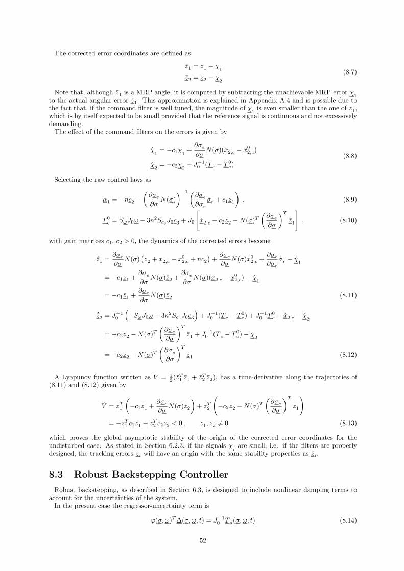
The corrected error coordinates are defined as
z1 = z1 − χ1
z2 = z2 − χ2
(8.7)
Note that, although z1 is a MRP angle, it is computed by subtracting the unachievable MRP error χ1
to the actual angular error z1. This approximation is explained in Appendix A.4 and is possible due tothe fact that, if the command filter is well tuned, the magnitude of χ
1is even smaller than the one of z1,
which is by itself expected to be small provided that the reference signal is continuous and not excessivelydemanding.The effect of the command filters on the errors is given by
χ1= −c1χ1
+∂σe
∂σN(σ)(x2,c − x0
2,c)
χ2= −c2χ2
+ J−10 (T c − T 0
c)
(8.8)
Selecting the raw control laws as
α1 = −nc2 −(∂σe
∂σN(σ)
)−1(∂σe
∂σr
σr + c1z1
)
, (8.9)
T 0c = SωJ0ω − 3n2Sc3J0c3 + J0
[
x2,c − c2z2 −N(σ)T(∂σe
∂σ
)T
z1
]
, (8.10)
with gain matrices c1, c2 > 0, the dynamics of the corrected errors become
˙z1 =∂σe
∂σN(σ)
(z2 + x2,c − x0
2,c + nc2)+
∂σe
∂σN(σ)x0
2,c +∂σe
∂σr
σr − χ1
= −c1z1 +∂σe
∂σN(σ)z2 +
∂σe
∂σN(σ)(x2,c − x0
2,c)− χ1
= −c1z1 +∂σe
∂σN(σ)z2 (8.11)
˙z2 = J−10
(
−SωJ0ω + 3n2Sc3J0c3
)
+ J−10 (T c − T 0
c) + J−10 T 0
c − x2,c − χ2
= −c2z2 −N(σ)T(∂σe
∂σ
)T
z1 + J−10 (T c − T 0
c)− χ2
= −c2z2 −N(σ)T(∂σe
∂σ
)T
z1 (8.12)
A Lyapunov function written as V = 12 (z
T1 z1 + zT2 z2), has a time-derivative along the trajectories of
(8.11) and (8.12) given by
V = zT1
(
−c1z1 +∂σe
∂σN(σ)z2
)
+ zT2
(
−c2z2 −N(σ)T(∂σe
∂σ
)T
z1
)
= −zT1 c1z1 − zT2 c2z2 < 0 , z1, z2 6= 0 (8.13)
which proves the global asymptotic stability of the origin of the corrected error coordinates for theundisturbed case. As stated in Section 6.2.3, if the signals χ
iare small, i.e. if the filters are properly
designed, the tracking errors zi will have an origin with the same stability properties as zi.
8.3 Robust Backstepping Controller
Robust backstepping, as described in Section 6.3, is designed to include nonlinear damping terms toaccount for the uncertainties of the system.In the present case the regressor-uncertainty term is
ϕ(σ, ω)T∆(σ, ω, t) = J−10 T d(σ, ω, t) (8.14)
52

where the regressor is a constant matrix J−10 .
Again, the procedure starts by defining the proper error coordinates
z1 = σe (8.15)
z2 = ω − x2,c (8.16)
where x2,c is, again, a filtered version of x02,c, which is defined exactly as in (8.6).
Having the disturbance term into account, the dynamics of these coordinates are
z1 =∂σe
∂σN(σ) (ω + nc2) +
∂σe
∂σr
σr (8.17)
z2 = J−10
(
−SωJ0ω + 3n2Sc3J0c3
)
+ J−10 T c + J−1
0 T d − x2,c (8.18)
Defining zi and χias in (8.7) and (8.8), respectively, and building the raw control signals as
α1 = −nc2 −(∂σe
∂σN(σ)
)−1(∂σe
∂σr
σr + c1z1
)
, c1 > 0 (8.19)
T 0c = SωJ0ω − 3n2Sc3J0c3 + J0
[
x2,c − c2z2 − sz2 −N(σ)T(∂σe
∂σ
)T
z1
]
, c2 > 0 (8.20)
with the nonlinear damping term
s = J−10 κ(J−1
0 )T = J−10 κJ−1
0 , κ = κT > 0 (8.21)
we obtain the following compensated error dynamics
˙z1 = −c1z1 +∂σe
∂σN(σ)z2 (8.22)
˙z2 = J−10
(
−SωJ0ω + 3n2Sc3J0c3
)
+ J−10 (T c − T 0
c) + J−10 T 0
c + J−10 T d − x2,c − χ
2
= −c2z2 − J−10 κJ−1
0 z2 + J−10 T d −N(σ)T
(∂σe
∂σ
)T
z1 (8.23)
Defining a Lyapunov candidate, again, as V = 12 (z
T1 z1 + zT2 z2), its time-derivative yields
V = zT1
(
−c1z1 +∂σe
∂σN(σ)z2
)
+ zT2
(
−c2z2 − J−10 κJ−1
0 z2 + J−10 T d −N(σ)T
(∂σe
∂σ
)T
z1
)
= −zT1 c1z1 − zT2 c2z2 − zT2 J−10 κJ−1
0 z2 + zT2 J−10 T d
= −zT1 c1z1 − zT2 c2z2 −(
J−10 z2 −
κ−1T d
2
)T
κ
(
J−10 z2 −
κ−1T d
2
)
+TT
d κ−1T d
4
≤ −zT1 c1z1 − zT2 c2z2 +TT
d κ−1T d
4(8.24)
From this it can be concluded that zi is input-to-state stable with respect to T d. As previously stressed,a proper design of the command filters will render small χ
i, which will imply the equivalence of stability
properties between the compensated and the tracking errors. The greater the values chosen for entriesof the matrix κ the smallest the compact set around the origin to which the error coordinates willasymptotically converge. The disturbance, of course, has to be bounded - property that is proved inAppendix B for all the considered uncertain scenarios.
8.4 Modular Adaptive Backstepping Controller
As explained in Section 7.1, the modular adaptive design is very similar to the robust one, in the sensethat it uses nonlinear damping terms, in this case, to account for estimation errors. This estimation isdone separately by an observer and, considering the model (8.1), the parameter being estimated is thedisturbance torque
ϕ(σ, ω)T θ(σ, ω, t) = J−10 T d(σ, ω, t) (8.25)
53

The design procedure for the tracking problem begins, as always, with the definition of the errorcoordinates
z1 = σe (8.26)
z2 = ω − x2,c (8.27)
where x2,c is the output of the command filtering of x02,c, which is given by
x02,c = α1 − χ
2(8.28)
χ2is a correction term, due to the action of the filter, which will be defined later.
The compensated tracking error coordinates are
z1 = z1 − χ1, z2 = z2 − χ
2(8.29)
where the correction terms for the effect of the command filtering have the following dynamics
χ1= −c1χ1
+∂σe
∂σN(σ)(x2,c − x0
2,c) (8.30)
χ2= −c2χ2
+ J−10 (T c − T 0
c) (8.31)
The raw control laws are defined as
α1 = −nc2 −(∂σe
∂σN(σ)
)−1(∂σe
∂σr
σr + c1z1
)
T 0c = SωJ0ω − 3n2Sc3J0c3 + J0
[
x2,c − c2z2 − sz2 −N(σ)T(∂σe
∂σ
)T
z1
]
− Td
(8.32)
with the gain matrices c1, c2 > 0. The nonlinear damping term is given by
s = J−10 κJ−1
0 , κ = κT > 0 (8.33)
Computing dynamics of the compensated errors for the closed-loop system gives
˙z1 =∂σe
∂σN(σ)
(z2 + x2,c − x0
2,c + nc2)+
∂σe
∂σN(σ)(α1 − χ
2) +
∂σe
∂σr
σr − χ1
= −c1z1 +∂σe
∂σN(σ)z2 (8.34)
˙z2 = J−10
(
−SωJ0ω + 3n2Sc3J0c3
)
+ J−10 (T c − T 0
c) + J−10 T 0
c + J−10 T d − x2,c − χ
2
= −c2z2 − J−10 κJ−1
0 z2 + J−10 T d −N(σ)T
(∂σe
∂σ
)T
z1 (8.35)
Let a control Lyapunov function for this problem be written as
V =1
2zT1 z1 +
1
2zT2 z2 (8.36)
Its time-derivative along the trajectories of (8.34) and (8.35) is
V = zT1
(
−c1z1 +∂σe
∂σN(σ)z2
)
+ zT2
(
−c2z2 − J−10 κJ−1
0 z2 + J−10 T d −N(σ)T
(∂σe
∂σ
)T
z1
)
= −zT1 c1z1 − zT2 c2z2 − zT2 J−10 κJ−1
0 z2 + zT2 J−10 T d
= −zT1 c1z1 − zT2 c2z2 −(
J−10 z2 −
κ−1T d
2
)T
κ
(
J−10 z2 −
κ−1T d
2
)
+T
T
d κ−1T d
4
≤ −zT1 c1z1 − zT2 c2z2 +T
T
d κ−1T d
4(8.37)
which implies that, for a bounded estimation error, the compact set to which the compensated error con-verges can be made arbitrarily small by setting the robustness gain κ sufficiently large. This boundednesscan be achieved, for a bounded disturbance, by imposing limits in the estimation through the use of theprojection operator in the estimation law. As mentioned before, the correct tunning of the commandfilters ensures small χi, which renders the tracking errors the same input-to-state stability propertiesproved for the compensated ones.
54

8.4.1 Nonlinear Extended State Observer
According to literature studied, and as described in Section 7.1.1, the Nonlinear Extended State Ob-server is one of the most suitable estimators for time-variable disturbances. In the present case, sincethe disturbance appears only in the dynamics equation, the estimator can be designed in a reduced orderform as
˙ω = Proj(
−J−10 ω × J0ω + 3n2J−1
0 c3(σ)× J−10 c3(σ) + J−1
0 T c + J−10 ξ − β1fal(ω, α1, δ1)
)
˙ξ = Proj (−β2fal(ω, α2, δ2))
(8.38)
where the extra state is the estimated disturbance torque
T d = ξ (8.39)
The estimation error is writtenω = ω − ω (8.40)
and the nonlinear gain is
fal(ω, αi, δi) =
fal(ω1, αi, δi)fal(ω2, αi, δi)fal(ω3, αi, δi)
, i = 1, 2 (8.41)
with
fal(ωj , αi, δi) =
|ωj |αi sign(ωj) , |ωj | > δi
ωj
δ1−αi
i
, |ωj | ≤ δi(8.42)
The estimator dynamics (8.38) can be expressed in terms of estimation error by
˙ω = J−10 ξ − β1fal(ω, α1, δ1)
˙ξ = −h(σ, ω, t)− β2fal(ω, α2, δ2)
(8.43)
withh(σ, ω, t) = T d (8.44)
If αi = 1 then (8.43) becomes[˙ω˙ξ
]
=
[
−β1 J−10
−β2 0
] [ω
ξ
]
−[0I
]
h(σ, ω, t) (8.45)
For diagonal matrices βi, the linear estimator (8.45) allows us to place the poles, for a diagonal matrixJ−10 , using the characteristic polynomial
∆j(s) = s2 + β1js+ β2jJ−10j
, j = 1, 2, 3 (8.46)
where Aj is the jth diagonal element of A.The poles can be chosen, for example, according to bandwidth criteria. Of course, for the estimator to
be stable, both β1 and β2J−10 have to be positive. To understand the gain role on the estimation, analyze
the linear case (8.45) in steady-state, that is
0 = −β1ω + J−10 ξ
0 = −β2ω − h(σ, ω, t)(8.47)
which rearranged givesω = −β−1
2 h(σ, ω, t) , ξ = −J0β1β−12 h(σ, ω, t) (8.48)
The identities (8.48) reveal that, for ω to be small, β2 must have large values and, for ξ to be minimized,not only β2 must be large, but also β1 must be defined as small as possible. Looking at (8.46) this meansthat the estimator target dynamics will have to be defined with a high natural frequency but very lowdamping ratio.As for the nonlinear parameters αi and δi, they are introduced to increase the estimator performance
for a varying disturbance. A small αi decreases the steady state error, while a small δi increases theestimation gain in an increasingly smaller region around the origin improving the tracking performanceof the estimator.
55

8.5 Integrated Adaptive Backstepping Controller
Due to the time-varying nature of the disturbance torque, the integrated adaptive algorithm had tobe modified to include robustness terms, as described in Section 7.2.3. The resulting design is almostidentical to the modular one, using instead a tracking error based integrated estimator.The design can be summarized as using the control laws
x02,c = −nc2 −
(∂σe
∂σN(σ)
)−1(∂σe
∂σr
σr + c1z1
)
− χ2
(8.49)
T 0c = SωJ0ω − 3n2Sc3J0c3 + J0
[
x2,c − c2z2 − sz2 −N(σ)T(∂σe
∂σ
)T
z1
]
− Td (8.50)
s = J−10 κJ−1
0 , κ = κT > 0 (8.51)
with c1, c2 > 0,
z1 = z1 − χ1, z2 = z2 − χ
2(8.52)
and
χ1= −c1χ1
+∂σe
∂σN(σ)(x2,c − x0
2,c) (8.53)
χ2= −c2χ2
+ J−10 (T c − T 0
c) (8.54)
As for the estimation update law, it is given by
˙T d = Proj
(ΓJ−1
0 z2)
(8.55)
where the projection operator is, once again, used to ensure boundedness of the estimation error.Notice that the error driving the estimation is the compensated one. This, when the saturation limits
in the command filters are achieved, avoids the unlearning of the estimation law since the compensatederror will, in such case, converge to zero while the tracking error is increasing.
8.6 Immersion and Invariance Adaptive Backstepping Controller
The last adaptive law here applied is the I&I adaptive backstepping, presented in Section 7.4. Inorder to obtain a fair comparison between control laws, and although the I&I design does not need theinclusion of nonlinear damping terms for stability, the control law is kept equal to the modular adaptiveand integrated adaptive backstepping. This leaves us the task of designing an I&I estimator. It starts bydefining the off-the-manifold coordinates
η = T d − T d + β(ω) (8.56)
which has the dynamics
η =˙T d − T d +
∂β(ω)
∂ωω (8.57)
Using control laws similar to (8.32) which are given by
x02,c = −nc2 −
(∂σe
∂σN(σ)
)−1(∂σe
∂σr
σr + c1z1
)
− χ2
T 0c = SωJ0ω − 3n2Sc3J0c3 + J0
[
x2,c − c2z2 − sz2 −N(σ)T(∂σe
∂σ
)T
z1
]
−(
Td + β(ω))
(8.58)
with gain matrices c1, c2 > 0 and nonlinear damping term
s = J−10 κJ−1
0 , κ = κT > 0 (8.59)
56
then (8.57) becomes
η =˙T d − T d +
∂β(ω)
∂ω
(
−J−10 SωJ0ω + 3n2J−1
0 Sc3J0c3 + J−10 (T c − T 0
c) + J−10 T 0
c + J−10 T d
)
=˙T d − T d +
∂β(ω)
∂ω
(
−c2z2 − sz2 −N(σ)T(∂σe
∂σ
)T
z1 + x2,c + J−10 (T c − T 0
c)− J−10 η
)
=˙T d − T d +
∂β(ω)
∂ω
(
−c2z2 − sz2 −N(σ)T(∂σe
∂σ
)T
z1 + x2,c + χ2− J−1
0 η
)
(8.60)
Defining the update law as
˙T d = −∂β(ω)
∂ω
(
−c2z2 − sz2 −N(σ)T(∂σe
∂σ
)T
z1 + x2,c + χ2
)
(8.61)
renders
η = −T d −∂β(ω)
∂ωJ−10 η (8.62)
In this case, because the regressor is constant, β(ω) admits the solution
β(ω) = γ
∫ ω
0
J−10 dχ = γJ−1
0 ω , γ > 0 (8.63)
Like before, the compensated tracking errors are
z1 = z1 − χ1, z2 = z2 − χ
2(8.64)
Being the effect of the command filters given by
χ1= −c1χ1
+∂σe
∂σN(σ)(x2,c − x0
2,c) (8.65)
χ2= −c2χ2
+ J−10 (T c − T 0
c) (8.66)
where the compensated errors have the dynamics
˙z1 =∂σe
∂σN(σ)
(z2 + x2,c − x0
2,c + nc2)+
∂σe
∂σN(σ)x0
2,c +∂σe
∂σr
σr − χ1
= −c1z1 +∂σe
∂σN(σ)z2 (8.67)
˙z2 = J−10
(
−SωJ0ω + 3n2Sc3J0c3
)
+ J−10 (T c − T 0
c) + J−10 T 0
c + J−10 T d − x2,c − χ
2
= −c2z2 − J−10 κJ−1
0 z2 − J−10 η −N(σ)T
(∂σe
∂σ
)T
z1 (8.68)
Consider the following control Lyapunov function
V = zT1 z1 + zT2 z2 + ηT η (8.69)
where its time-derivative along the trajectories of (8.62), (8.67) and (8.68) is
V = 2zT1
(
−c1z1 +∂σe
∂σN(σ)z2
)
+ 2zT2
(
−c2z2 − J−10 κJ−1
0 z2 − J−10 η −N(σ)T
(∂σe
∂σ
)T
z1
)
+ 2ηT(
−T d − γJ−10 J−1
0 η)
= −2zT1 c1z1 − 2zT2 c2z2 − 2zT2 J−10 κJ−1
0 z2 − 2zT2 J−10 η − 2ηT T d − 2γηTJ−1
0 J−10 η
= −2zT1 c1z1 − 2zT2
(
c2 −1
2ΛΛ + J−1
0 κJ−10
)
z2 −(Λ−1J−1
0 η + Λz2)T (
Λ−1J−10 η + Λz2
)
− ηTJ−10
(γI − Λ−1Λ−1
)J−10 η − γ
(
J−10 η +
1
γJ0T d
)T (
J−10 η +
1
γJ0T d
)
+1
γT
T
d J0J0T d
57

≤ −2zT1 c1z1 − 2zT2
(
c2 −1
2ΛΛ + J−1
0 κJ−10
)
z2 − ηTJ−10
(γI − Λ−1Λ−1
)J−10 η
+1
γT
T
d J0J0T d (8.70)
with Λ = ΛT > 0.Let
c2 = c2 −1
2ΛΛ + J−1
0 κJ−10 > 0 , γI − Λ−1Λ−1 ≥ 0 (8.71)
then (8.70) becomes
V ≤ −2zT1 c1z1 − 2zT2 c2z2 +1
γT
T
d J0J0T d (8.72)
which proves the convergence of the compensated tracking error to a compact set around the origin.The higher the estimation gain γ, the smaller this set will be, provided that the time-derivative of thedisturbance is bounded - property that was proved in Appendix B. A proper design of the commandfilters ensures the convergence of the tracking error to the same compact set. Additionally, by Lemma 7.2we have J−1
0 η → 0 which implies T d + β → T d.
8.7 Gain Selection
All the controller and estimator gains shall now be chosen. In order to make a fair comparison betweencontrollers, the error feedback gains c1 and c2 are selected equal for all designs. The same happens withthe robustness gain κ for the ones that have nonlinear damping terms. The Backstepping controllerdesigns require only that c1 and c2 be positive definite to stabilize the nominal model. It is commonpractice to choose the inner loop gains higher than the outer loop ones. Following this rule the selectedgains are
c1 =
0.1 0 00 0.1 00 0 0.1
, c2 =
1 0 00 1 00 0 1
(8.73)
Since the Backstepping design is not performance based, but instead stability based, it is usually nottrivial to assess the performance of the closed-loop system. To evaluate such performance, consider thedynamics (8.11) and (8.12) written in state space form as
[˙z1˙z2
]
=
[−c1 W (σ, σr)
−W (σ, σr)T −c2
] [z1z2
]
(8.74)
where W (σ, σr) =∂σe
∂σ N(σ). For near perfect tracking (σ ≈ σr) we have W ≈ −1/4I. This allows
the decoupling of (8.74) into three second order systems, one for each angular component, each with acharacteristic polynomial
∆i(s) = s2 + (c1i + c2i)s+ c1ic2i + (WTW )i , i = 1, 2, 3 (8.75)
where Ai is here the ith element of the diagonal of A. Computing the poles yields
pi = −0.176; −0.924 rad/s (8.76)
revealing two first order systems, the inner and the outer loop, with time constants of 1.08 s and 5.68 s,respectively.This analysis leads to the conclusion that, for not excessively demanding reference signals, i.e. whenever
the tracking error is small, the performance should be equivalent to the one of a system with poles at(8.76).Turning the attention to the robustness added designs, from (8.23) it is clear that a positive gain κ acts
as a reinforcement of c2, this way the value for this gain has to be chosen the same order of magnitudeas the inner loop feedback gain. It was selected as
κ = J0KJ0 with K =
1 0 00 1 00 0 1
(8.77)
58

being the equivalent inner loop gain for the robust design: c2+K. With this, the poles move from (8.76)to −0.133,−1.967 rad/s.To design the nonlinear extended state observer gains and parameters one can follow the indications
given in Section 8.4.1: the gain β2 must be chosen larger than β1 in order to reduce the steady-stateestimation errors; a small parameter α (< 1) has a similar effect and additionally decreases the estimationgain for larger errors, avoiding violent behavior in such case; the gain bounding parameter δ should beselected small (< 1) so that the estimator has a very high gain in a small region around the origin,augmenting the estimation tracking performance. Following these trends, and after an iterative process,it was selected as
β1 =
1 0 00 1 00 0 1
, β2 = BJ0 with B =
5 0 00 5 00 0 5
(8.78)
α1 = 0.2 , α2 = 0.4 , δ1 = 0.1 , δ2 = 0.3 (8.79)
The designed gains, for the equivalent Luenberger observer (αi = 1), would yield ωn = 2.24 rad/s andζ = 0.22. In such case, the estimator has a slightly faster dynamics than the closed-loop nonadaptivesystem (8.76). As expected the price of low steady-state error is a lightly damped estimation performance.Nevertheless, the introduction of the nonlinear gain features not only completely eliminates this drawbackbut also makes the estimator faster near the origin. For small state estimation error (ωj ≤ δ1 < δ2) theestimator is linear and has the characteristic polynomial for each angular error component
∆j(s) = s2 +β1j
δ1−α1
1
s+Bj
δ1−α1
1
(8.80)
which has poles with ωn = 3.21 rad/s and ζ = 0.98.The tuning of an integrated adaptive backstepping design, although requiring the selection of only one
positive gain (Γ), is not trivial. As it has been proved in (Krstic et al., 1995), the increase of Γ makes theestimation convergence faster but, for large values, degrades the controller transient performance. Thisinfluence is not clear, making it very difficult to find a good trade-off. In a trial-and-error process theselected value was
Γ = GJ0 with G =
15 0 00 15 00 0 15
(8.81)
Contrarily to the integrated adaptive backstepping the I&I adaptive design is much easier to tune.Because the estimator is designed according to the closed-loop dynamics, forming a cascade of two stablesystems, the increase of the gain γ not only leads to a faster estimation, but also improves the closed-loopdynamic performance. The gain was chosen to be
γ = 50 (8.82)
Although (8.82) might appear large, it must be noted that in the off-the-manifold coordinate dynamics(8.62) it is multiplied by J−1
0 J−10 . The choice of γ was then highly dependent on the inertia matrix of
the nominal spacecraft model.To make sure the gain obeys the conditions (8.71) without explicitly computing a value for Λ, one can
join the two inequalities yielding
c2 + J−10 κJ−1
0 >I
2γ(8.83)
which is clearly satisfied for (8.73) and (8.82) regardless of the magnitude of J−10 κJ−1
0 (by definition ofκ this term is guaranteed to be positive definite).
59

Chapter 9
Simulation and Performance
Analysis
In order to evaluate the performance of the control laws derived in the preceding chapter, a setof simulation scenarios including different uncertainties and disturbances is designed. Then,an attitude trajectory is defined. Finally, the simulation results are presented and discussed.
9.1 Uncertainty Scenarios
In this section three hypothetical uncertainty situations are described. Although they might be insome cases extreme in the sense that, with the robustness of space-certified systems, they would veryhardly occur, it must be noted that their main intent is to test the limits of performance of the builtcontrollers. Nevertheless, whenever possible, the presented situations will be conceived with support ofrealistic dimensions and parameters.The chosen scenarios are: constant inertial mismatch, uncontrolled reaction wheel and moving payload.
9.1.1 Constant Inertial Mismatch
The first situation considered is a constant mismatch in the inertia matrix. Here it is assumed thatthe controller is designed with an inertia matrix that is different from the real one, which is constant.This can be caused by a variety of circumstances, among them: pre-launch imprecise inertial measure-ments; rupture or mechanical part displacement; fuel consumption and tank level management; andinstrument/structure deployment.In (Ziemer, Cubbin, Choueiri, Oraevsky, & Dokukin, 1996) the errors described for the pre-launch
inertial measurements of a spacecraft of similar mass and size to the studied one are 1.5% for the momentsof inertia and 5% for the products of inertia.Assume that during such measurements the principal inertial axes were estimated with an error de-
scribed by a 3-2-1 Euler-angle rotation of (θ1, θ2, θ3) = (10, 10, 10) deg. The measured inertia tensor isgiven by (Schaub & Junkins, 2002)
J0 = CPP′
J(CPP′
)T (9.1)
where J is the real inertia tensor, that was computed in Section 2.2 as
J =
3.083 0 00 3.083 00 0 2.083
Kgm2 (9.2)
The measured tensor is then
J0 =
3.053 0.030 0.1680.030 3.054 −0.1660.168 −0.166 2.143
Kgm2 (9.3)
which represents an error of about 1% in the first two moments of inertia and 3% in the third.Using the uncertainty model representation deduced in Section 4.1, the true inertia is given in terms of
the known part byJ = J0 +∆J (9.4)
60

then the inertial error is
∆J =
0.030 −0.030 −0.168−0.030 0.029 0.166−0.168 0.166 −0.059
Kgm2 (9.5)
9.1.2 Uncontrolled Reaction Wheel
For the second scenario we consider a Reaction Wheel (RW) failure situation. Suppose one of the fourreaction wheels of the spacecraft is uncontrolled and saturated at its maximum speed. It will cause adisturbance torque similar to the one described in Section 4.2.1 for a rotating disk.The reaction wheel specifications this mission were taken from (Bakker, 2009) and are shown in Ta-
ble 9.1. The flywheel (rotating disk) dimensions and mass were assumed based on typical values forsimilar devices, since there is no specified information for it in this case.
Table 9.1: Reaction Wheels Specifications (Bakker, 2009).
Total mass 1.986KgDimensions 0.118× 0.118× 0.115m3
Maximum angular momentum 0.65NmsMaximum torque 0.05NmSpeed range ±4200 rpmFlywheel mass 1KgFlywheel radius 0.055mFlywheel thickness 0.03m
(a) Configuration
l
l
l
β
β
(b) Geometry details
Figure 9.1: Reaction wheel configuration (Bakker, 2009).
In (Bakker, 2009) the RW configuration was studied and it was concluded that the Square-based-pyramidGeometry and Equilateral Tetrahedron Geometry were equivalent and showed better performance thanthe classical one. For this test it was chosen to have an Equilateral Tetrahedron Geometry (Figure 9.1a).The details of this geometry are shown in Figure 9.1b and the geometrical relations are
β = 19.471 deg , a =1
2√3l , b =
√3
2l (9.6)
It is assumed that each flywheel1 has its center of mass in the center of a surface of the tetrahedron.Furthermore, the center of the tetrahedron is the origin of the Body reference frame B (Figure 9.1a).
1From here on we will use the term Reaction Wheel to refer to the rotating disk of the actuation device.
61

Since in (Bakker, 2009) the author does not provide absolute dimensions for the configuration, weassume a triangle side of l = 0.3m. The resulting RW positions are shown in Table 9.2. All the positionvectors are written in B coordinates.
Table 9.2: Reaction wheels position for l = 0.3m.
eB1 (m) eB2 (m) eB3 (m)
RRW1
0.043 0 0.014R
RW2−0.022 0.038 0.014
RRW3
−0.022 −0.038 0.014R
RW40 0 −0.107
As it was referred in Section 4.2.1, in order to transform the inertia matrix of the disk from its referenceframe A′ to the Body frame B we need the direction cosine matrix of such rotation. This can be done byfinding a vector of Euler angles that transforms A′ to B, or the inverse, in a 3-2-1 rotation scheme. Theframe A′ is defined as having the third axis coincident to the rotation axis of the wheel (in the positivedirection) and the remaining axes coplanar to the disk plane. Table 9.3 presents possible Euler anglevectors to transform B into the reference frame of each RW.
Table 9.3: Possible Euler angles from B to A′ with 3-2-1 rotation order.
θ3 (deg) θ2 (deg) θ1 (deg)
RW1 0 90− β 0RW2 30 0 β − 90RW3 −30 0 90− βRW4 0 0 180
For simplicity, and since the control allocation is not treated in this thesis, it is assumed that themaximum available actuation torque remains the same as in the nominal case. It will also be assumedthat the overall known inertia tensor computed in Section 2.2 already includes the moments of inertia ofall four reaction wheels.
9.1.3 Moving Payload
The last scenario introduces the effect of time-varying inertia cased by a moving object inside thespacecraft.Imagine that as payload there is a scientific instrument that has a moving part that was not accounted
for when designing the attitude control system. Furthermore, consider that this part has approximatelya rectangular cuboid form and moves around its own center of mass in a one-axis-rotation motion. Thedisturbance caused by such part is similar to the one modeled in Section 4.2.2.In (Juang, 2004) the attitude disturbance caused by a moving mirror inside the NASA’s GIFTS (Geo-
stationary Imaging Fourier Transform Spectrometer) is deduced and studied. Here, we consider a similarinstrument but with smaller dimensions.Although the on-board spectropolarimeter SPEX is not referred to having any moving part, suppose
it has a moving glass mirror (Figure 9.2b) with the properties presented in Table 9.4. The vector Rb
(Figure 9.2a) represents the position of the mirror’s center of mass in B coordinates and (θ1, θ2, θ3) isthe set of Euler angles necessary to transform B to A′ using a 3-2-1 rotation order. The latter referenceframe is fixed in B and is defined as having the third axis coincident to the rotation axis of the mirrorand the origin in its center of mass. A third reference frame A is defined as being fixed to the mirrorand, similarly to A′, as having the third axis overlapped with the rotation axis of b and the origin in itscenter of mass.Assume the mirror has a sinusoidal motion about the third axis of A described by
θ(t) = Ab sin
(2π
Tbt
)
, ωb(t) = Ab2π
Tbcos
(2π
Tbt
)
, ωb(t) = −Ab
(2π
Tb
)2
sin
(2π
Tbt
)
(9.7)
where Ab, the peak angular amplitude of the movement, and Tb, the period, are presented in Table 9.4.These angular motion functions, as explained in Section 4.2.2, are used to compute the direction cosine
62

matrix from A to A′ and, together with CA′B and Rb, the inertia tensor and its time-derivative in Bcoordinates.Like in the previous scenario, it is assumed that the nominal inertia tensor computed in Section 2.2
already accounts for the mirror in its static position, which is given by the angle θ0.
Table 9.4: Mirror (part b) properties.
Dimensions l × w × h 0.005× 0.05× 0.05m3
Mass 0.03KgPosition Rb [0.30 0.20 0.20] mOrientation (θ1, θ2, θ3) [0 45 45] degMovement Peak Amplitude Ab 45 degMovement Period Tb 15 sθ0 45 deg
eA1
eA2
eA3
ωb
b
lw
h
eA′
2
eA′
1
θ
(a) Defining frames and dimensions.
eB1
eB2eB3
45
45
b
eA′
2
eA′
3
eA′
1
Rb
(b) Orientation and position in B.
Figure 9.2: Moving mirror (part b).
9.2 Simulated Attitude Trajectory
As it was described in Chapter 2, the FAST-D spacecraft is being conceived to collect atmosphericdata. To accomplish so, an attitude scanning maneuver is here defined in terms of MRP. Although inthe project literature only a “yaw oscillating movement” (Maessen & Laan, 2008) is described, we willassume the need for a more general “sweeping” reference.The trajectory chosen for simulation starts from nadir pointing σ0 and steers the spacecraft to orient
with σ1. Then, after a period of rest, the vehicle begins an oscillating movement with a peak-to-peakamplitude of 60 deg between σ1 and σ2. This reference is displayed in Figure 9.3 both in MRP and Eulerangles. The σ points that define it are
σ1 =k1‖k1‖
tan
(30 deg
4
)
, σ2 =k2‖k2‖
tan
(30 deg
4
)
(9.8)
withk1 =
[−1 1 0.5
]T, k2 =
[1 −1 −0.5
]T(9.9)
The angular rate of the unfiltered ramp is 0.3 deg/s, the time constant used for the low-pass filteringwas τ = 30 s and the period of the scanning oscillations is T = 300 s.
63

σ3rσ2rσ1r
σ
Time [s]0 100 200 300 400 500 600 700 800 900 1000 1100
−0.1
−0.05
0
0.05
0.1
(a) Modified Rodrigues Parameters
θ3rθ2rθ1r
EulerAngles
[deg]
Time [s]0 100 200 300 400 500 600 700 800 900 1000 1100
−20−15−10−50510152025
(b) Euler Angles
Figure 9.3: Attitude reference trajectory.
9.3 Controllers Performance
Before presenting the performance assessment of the designed controllers in all defined scenarios, wefirst introduce some important points for the discussion of results.Although the designed uncertainty scenarios might look in some points extreme, the resulting distur-
bance torques are, under normal operation values of angular rate, considerably low. Hence, the trackingerror resulting from them will be in most cases very small, being at times difficult to perceive in thetrajectory-following plots. The referred error will, therefore, be displayed as a one-angle pointing errorexpressed in arcsec. This representation is given by
σe = ke tan
(θe4
)
⇒ θe = 4arctan (‖σe‖) (9.10)
Note that this angle is the most convenient to evaluate the error with respect the requirements definedin Section 2.3
θe ≤ 30 arcsec , |ωe| = |z2| ≤ 1 arcsec/s (9.11)
The pointing accuracy and stability definitions used in this analysis are in accordance to the EuropeanSpace Agency (ESA) Pointing Error Handbook (Dungate, 1993). The defined requirements are espe-cially important during data acquisition periods, i.e. during steady-pointing or scanning maneuvers. Toevaluate and compare the tracking performance in these situations we shall use the Root Mean Square(RMS) of the error. The estimation error of the adaptive laws will also be analyzed through the RMS ofits 2-norm.The control effort will be compared using the actuation absolute workload, quantity that is computed by
considering the energy exchanged between the actuators and the spacecraft as always positive. This meansthat the actuators consume power either to accelerate and decelerate the spacecraft (in any direction).Then, the power needed to apply a torque T c to the spacecraft at ω is
P (t) =
3∑
i=1
|ωi(t)Tci(t)| , (9.12)
64

The absolute workload for an interval t ∈ [t1, t2] is computed as (Schaub & Junkins, 2002)
W =
∫ t2
t1
P (t)dt =
∫ t2
t1
3∑
i=1
|ωi(t)Tci(t)|dt . (9.13)
Table 9.5 displays the limits on the input signals and estimated states imposed by the command filtersand projection operators, respectively. See Appendices C.1 and C.2 for more details.
Table 9.5: Limits imposed on the input signals and estimated states.
Magnitude Rate
x2,c 1 deg/s 0.15 deg/s2
T c 0.05√
43 Nm 6Nm/s
ω 2 deg/s -
T c 0.1Nm -
In (Adams, Bruno, Shah, & Keller, 1998) the attitude control system of an earth observation smallsatellite was implemented at 10Hz. The controllers were here simulated at such frequency and, tominimize the error introduced by the model integration, the model states were propagated at 100Hz.For the simulated 650 km high circular orbit2 the orbital rate is n = 1.073e-3 rad/s.For the presentation and discussion of results the controllers will be referred to as: BS, Static standard
backstepping, RBS, Static robust backstepping, TF Integrated adaptive (tuning function) backstepping,NESO, Modular adaptive backstepping with nonlinear extended state observer and I&I, Immersion andinvariance adaptive backstepping.It should be noted that, for the presentation and comparison of the estimation performance of the I&I
adaptive law, the estimated disturbance, referred to as T d, is in fact the result of the sum T d+β, since itis this value that converges to the true value of T d when the off-the-manifold coordinate η goes to zero.The innovation plots of the nonlinear extended state observer can be found in Appendix E, and testify
the convergence of the observer for all the tested scenarios.
9.3.1 Nominal Performance
In this section the five designed controllers are compared in an uncertainty free scenario following thedefined trajectory.The plots from this simulations can be found in Appendix E.1. As can be seen from Figure E.1 all the
controllers follow both the angular trajectory and the angular rate virtual reference very closely, beingimpossible to distinguish the curves from the several control laws. The differences between them areonly visible at a arcsec scale, as shows the pointing error plot on Figure 9.4 and the rate error plot onFigure 9.5. It might be surprising that, despite having a higher inner loop gain due to the nonlineardamping terms, the static robust backstepping design (RBS) has a larger error than the standard design(BS). In fact, by raising the equivalent inner loop gain and leaving the angular loop gain unchanged, wemoved the faster poles further to the left and the slower ones to the right. As a result, although the rateloop is faster, the angle tracking became slightly slower due to the slower poles.Among the adaptive designs, from the estimation plots on Figure E.2(b), it is possible to recognize
the integrated adaptive behavior displayed by the tuning functions design (TF) and the immersion andinvariance law (I&I), which keep adapting whilst the tracking error is not null (hence, the adaptationdoes not cease during the scanning maneuver). On the contrary, the modular adaptive law (NESO)recognizes the null disturbance even when there is tracking error. Nevertheless, both the NESO andthe I&I show very close performances to the one of the RBS, which is natural since all these controllersinclude nonlinear damping terms. The TF controller, on the other hand, displays the worst tracking errorevolution, which confirms that, in the tuning of such Lyapunov update laws, a fast adaptation may costtracking performance. The described results can be confirmed by the error RMS of the entire trajectoryand of the specific periods of steady-pointing and scanning (Table 9.6).As it happened with the pointing error, the rate error from the NESO and I&I are overlapped with
the one from RBS, which has the same target behavior. Their rate performance is slightly better thanthe one of the BS, consequence of the shift suffered by the faster poles due to the introduction of thenonlinear damping term. The TF controller displays the best rate tracking of the five, consequence of
2The orbit defined for the FAST mission will be close to circular.
65

the Lyapunov-defined estimation law that keeps adapting even when the disturbance (matched in thedynamics equation) is null. This feature, however, degrades the angular tracking performance of thecontroller.All the control laws succeeded in keeping the error θe below 30 arcsec and the rate error |ωe| below
1 arcsec/s during steady-pointing and scanning periods, after the transient peaks.Due to very similar actuation torque profiles (Figure E.2(a)), the actuation workload used by the five
controlled systems is about the same, differing only in tenths of µJ (Table 9.7).
Table 9.6: Angular pointing error RMS θeRMSin the nominal scenario.
BS RBS TF NESO I&I
Entire Trajectory
θeRMS[arcsec] 8.343 9.855 12.422 9.916 10.282
Steady-pointing t ∈ [300, 500] s
θeRMS[arcsec] 0.009 0.012 0.018 0.012 0.012
Scanning Maneuver t ∈ [500, 1100] s
θeRMS[arcsec] 10.059 12.290 15.833 12.329 12.261
I&INESOTFRBSBS
θe[arcsec]
Time [s]0 100 200 300 400 500 600 700 800 900 1000 1100
0
5
10
15
20
25
30
35
40
Figure 9.4: Pointing angular error θe of all control laws in the nominal scenario.
I&INESOTFRBSBS
|ωe|[arcsec/s]
Time [s]0 100 200 300 400 500 600 700 800 900 1000 1100
0
1
2
3
4
5
6
Figure 9.5: Rate error norm of all control laws in the nominal scenario.
Table 9.7: Workload along the entire trajectory in the nominal scenario.
BS RBS TF NESO I&I
W [mJ ] 1.511 1.511 1.512 1.511 1.511
66

9.3.2 Constant Inertial Mismatch
This section analyzes the different controllers performances in the presence of a constant inertial mis-match as described in Section 9.1.1.The plots resulting from this simulation are in Appendix E.2. Again, all the σ and ω evolutions are
very close to the reference signals (Figures E.3(a) and E.3(b)), being impossible to draw conclusions fromthe plot of this parameter. Looking at a smaller scale at Figure 9.6, the pointing error curves revealthat the static controllers suffered a great decrease of performance, falling out of the desired boundsduring the scanning maneuver. However, the steady-pointing performance was the one to deteriorate themost (Table 9.8). Nevertheless, the error in static situation is still very small, which is easily explainedanalyzing the disturbance torque expression. In this scenario it is given by
T d(σ, ω) = −J0(∆J∗SωJ + J−10 Sω∆J)ω + 3n2J0(∆J∗Sc
3J + J−1
0 Sc3∆J)c3 + J0∆J∗T c , (9.14)
Two terms of (9.14) vanish as ω, T c → 0. In steady-pointing the angular rate is extremely small(ω = −nc2) and so is the control torque keeping the spacecraft in a constant and slow rotation. In suchcase the disturbing torque will be the same order of magnitude as the gravity gradient torque, which dueto the close-to-cubical form of the studied spacecraft, is nominally very small.The robust design (RBS), contrarily to the nominal case, performed better than the standard design
(BS) thanks to a higher gain in the dynamics loop, which is exactly where the disturbances occur. Writingthe Lyapunov function for the error as V = 1
2 (zT1 z1 + zT2 z2) its time-derivative for this case is
V = −zT1 c1z1 − zT2 cωz2 + zT2 J−10 T d (9.15)
which by squares completion yields
V = −zT1 c1z1 −(
z2 −c−1ω J−1
0 T d
2
)T
cω
(
z2 −c−1ω J−1
0 T d
2
)
+TT
d J−10 c−1
ω J−10 T d
4
≤ −zT1 c1z1 +TT
d J−10 c−1
ω J−10 T d
4(9.16)
where cω is the equivalent inner-loop gain. (9.16) proves that the MRP error z1 asymptotically convergesto a compact set around the origin given by
Ω =
z1 ∈ R
3 | ‖z1‖ <1
2
√
TTd J
−10 c−1
ω J−10 T d
cσ
, (9.17)
where cσ is the value of the diagonal elements of c1, which were selected equal. It is easy to see that, forthe same c1, J0 and T d, a larger gain cω results in smaller set Ω and, thus, in a smaller tracking error z1.For the standard design cω = c2 while in the robust law it is augmented to cω = c2 +K, explaining thesmaller error for the latter control design.The adaptive controllers all maintained the performance showed in the nominal scenario, revealing the
benefit of the dynamic feedback (Table 9.8). Again the NESO and the I&I had very close behaviors,having now the lowest errors of all five laws. The tuning functions design (TF) displays a clearly worseestimation than the other two adaptive laws (Figure E.4(b)), showing some coupling between the first and
the second components of T d. This is corroborated by the RMS of the estimation error from the threeidentifiers during the scanning maneuver after the estimation transitory peak. Such data is displayed inTable 9.9, where the error RMS is also compared to the total disturbance RMS. The TF estimator hasan error of 33% of the total disturbance RMS, which is much higher than the (about) 3% achieved bythe other two adaptive laws.The rate tracking performance was roughly maintained by all adaptive control laws, once again respect-
ing the limits outside the transient peaks in the beginning and ending of maneuvers, as shows Figure 9.7.The static laws, on the contrary, suffered a considerable increase of rate error, leaving the required boundduring the scanning movement.Finally, because the actuation torque used by the controllers was very close to the nominal case (Fig-
ure E.4(a)), the workload was about the same compared to such case (Table 9.10).
67

Table 9.8: Angular pointing error RMS θeRMSin the presence of constant inertial mismatch.
BS RBS TF NESO I&I
Entire Trajectory
θeRMS[arcsec] 23.831 18.872 12.436 9.937 10.294
Ratio to Nominal 2.856 1.915 1.001 1.002 1.001
Steady-pointing t ∈ [300, 500] s
θeRMS[arcsec] 0.375 0.232 0.018 0.011 0.012
Ratio to Nominal 43.426 19.374 0.991 0.989 0.997
Scanning Maneuver t ∈ [500, 1100] s
θeRMS[arcsec] 31.157 24.572 15.842 12.342 12.263
Ratio to Nominal 3.097 1.999 1.001 1.001 1.000
I&INESOTFRBSBS
θe[arcsec]
Time [s]0 100 200 300 400 500 600 700 800 900 1000 1100
0
10
20
30
40
50
60
70
80
Figure 9.6: Pointing error θe of all control laws in the presence of constant inertial mismatch.
I&INESOTFRBSBS
|ωe|[arcsec/
s]
Time [s]0 100 200 300 400 500 600 700 800 900 1000 1100
0
1
2
3
4
5
6
Figure 9.7: Rate error norm for all controllers in the presence of constant inertial mismatch.
Table 9.9: Estimation error RMS during scanning motion for t ∈ [505, 1100] s in the presence of constantinertial mismatch.
TF NESO I&I
TdRMS[µNm] 13.726 1.189 0.891
Ratio to TdRMS0.336 0.029 0.022
Table 9.10: Workload along the entire trajectory in the presence of constant inertial mismatch.
BS RBS TF NESO I&I
W [mJ ] 1.511 1.511 1.512 1.511 1.511
9.3.3 Uncontrolled Reaction Wheel
In this section we analyze the response of the system controlled by the designed laws when subjectedto a gyroscopic moment caused by a saturated RW. Considering the actuator configuration defined in
68
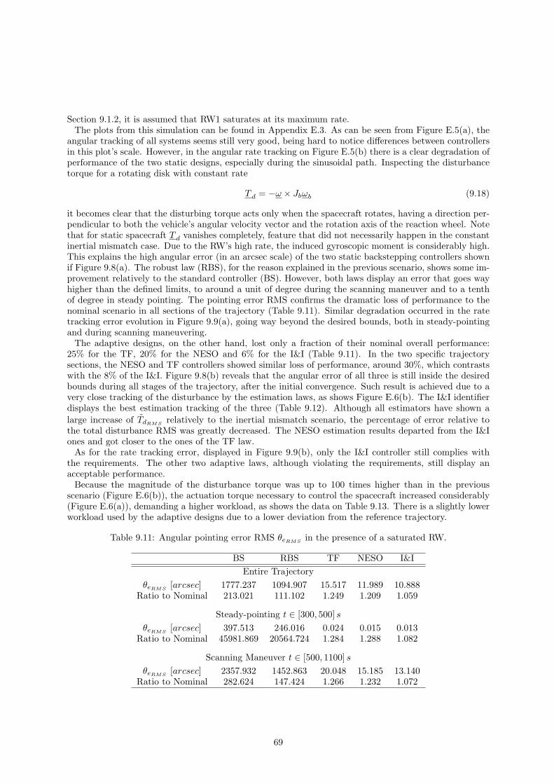
Section 9.1.2, it is assumed that RW1 saturates at its maximum rate.The plots from this simulation can be found in Appendix E.3. As can be seen from Figure E.5(a), the
angular tracking of all systems seems still very good, being hard to notice differences between controllersin this plot’s scale. However, in the angular rate tracking on Figure E.5(b) there is a clear degradation ofperformance of the two static designs, especially during the sinusoidal path. Inspecting the disturbancetorque for a rotating disk with constant rate
T d = −ω × Jbωb (9.18)
it becomes clear that the disturbing torque acts only when the spacecraft rotates, having a direction per-pendicular to both the vehicle’s angular velocity vector and the rotation axis of the reaction wheel. Notethat for static spacecraft T d vanishes completely, feature that did not necessarily happen in the constantinertial mismatch case. Due to the RW’s high rate, the induced gyroscopic moment is considerably high.This explains the high angular error (in an arcsec scale) of the two static backstepping controllers shownif Figure 9.8(a). The robust law (RBS), for the reason explained in the previous scenario, shows some im-provement relatively to the standard controller (BS). However, both laws display an error that goes wayhigher than the defined limits, to around a unit of degree during the scanning maneuver and to a tenthof degree in steady pointing. The pointing error RMS confirms the dramatic loss of performance to thenominal scenario in all sections of the trajectory (Table 9.11). Similar degradation occurred in the ratetracking error evolution in Figure 9.9(a), going way beyond the desired bounds, both in steady-pointingand during scanning maneuvering.The adaptive designs, on the other hand, lost only a fraction of their nominal overall performance:
25% for the TF, 20% for the NESO and 6% for the I&I (Table 9.11). In the two specific trajectorysections, the NESO and TF controllers showed similar loss of performance, around 30%, which contrastswith the 8% of the I&I. Figure 9.8(b) reveals that the angular error of all three is still inside the desiredbounds during all stages of the trajectory, after the initial convergence. Such result is achieved due to avery close tracking of the disturbance by the estimation laws, as shows Figure E.6(b). The I&I identifierdisplays the best estimation tracking of the three (Table 9.12). Although all estimators have shown a
large increase of TdRMSrelatively to the inertial mismatch scenario, the percentage of error relative to
the total disturbance RMS was greatly decreased. The NESO estimation results departed from the I&Iones and got closer to the ones of the TF law.As for the rate tracking error, displayed in Figure 9.9(b), only the I&I controller still complies with
the requirements. The other two adaptive laws, although violating the requirements, still display anacceptable performance.Because the magnitude of the disturbance torque was up to 100 times higher than in the previous
scenario (Figure E.6(b)), the actuation torque necessary to control the spacecraft increased considerably(Figure E.6(a)), demanding a higher workload, as shows the data on Table 9.13. There is a slightly lowerworkload used by the adaptive designs due to a lower deviation from the reference trajectory.
Table 9.11: Angular pointing error RMS θeRMSin the presence of a saturated RW.
BS RBS TF NESO I&I
Entire Trajectory
θeRMS[arcsec] 1777.237 1094.907 15.517 11.989 10.888
Ratio to Nominal 213.021 111.102 1.249 1.209 1.059
Steady-pointing t ∈ [300, 500] s
θeRMS[arcsec] 397.513 246.016 0.024 0.015 0.013
Ratio to Nominal 45981.869 20564.724 1.284 1.288 1.082
Scanning Maneuver t ∈ [500, 1100] s
θeRMS[arcsec] 2357.932 1452.863 20.048 15.185 13.140
Ratio to Nominal 282.624 147.424 1.266 1.232 1.072
69

RBSBS
θ e[arcsec]
Time [s]
0 100 200 300 400 500 600 700 800 900 1000 11000
500
1000
1500
2000
2500
3000
3500
4000
(a) Static controllers
I&INESOTF
θ e[arcsec]
Time [s]0 100 200 300 400 500 600 700 800 900 1000 11000
10
20
30
40
50
(b) Adaptive controllers
Figure 9.8: Angular pointing error θe in the presence of a saturated RW.
RBSBS
|ωe|[arcsec/s]
Time [s]0 100 200 300 400 500 600 700 800 900 1000 11000
50
100
150
200
250
300
350
400
(a) Static controllers
I&INESOTF
|ωe|[arcsec/s]
Time [s]0 100 200 300 400 500 600 700 800 900 1000 11000
1
2
3
4
5
6
(b) Adaptive controllers
Figure 9.9: Rate error norm in the presence of saturated RW.
70

Table 9.12: Estimation error RMS during scanning motion for t ∈ [505, 1100] s in the presence of asaturated RW.
TF NESO I&I
TdRMS[µNm] 46.653 32.834 13.705
Ratio to TdRMS0.010 0.007 0.003
Table 9.13: Workload along the entire trajectory in the presence of a saturated RW.
BS RBS TF NESO I&I
W [mJ ] 1.862 1.859 1.853 1.853 1.853
9.3.4 Moving Payload
The final tested scenario, described in Section 9.1.3, concerns the disturbance caused by a movingmirror from a spectrometer in the spacecraft’s payload. In this section the performances of the designedcontrollers are evaluated in the presence of such disturbance. The plots from this simulation can be foundin Appendix E.4.Similarly to all the previous simulations, the angular behavior of all systems is indistinguishable from
the reference in the σ plots, Figure E.7(a). Some trembling can, however, be perceived in the angularrate tracking in Figure E.7(b). If, as before, we analyze the disturbance torque expression, which is givenby
T d(σ, ω, t) = J0∆J∗(t)(−ω × J(t)ω + T c + T g(t)) + (−ω ×∆Jb(t)ω +∆T g(t))
− J0J−1(t)(ω × Jb(t)ωb +
˙∆Jb(t)(ω + ωb) + Jb(t)ωb)(9.19)
it will turn out to be dominated by the mirror’s angular acceleration term. This term, due to the smalldimensions of the moving piece, can be approximated by
T d ≈ −J0J−1Jbωb = −J0 (J
−10 +∆J∗)
︸ ︷︷ ︸
≈J−1
0
(Jb0 +∆Jb)︸ ︷︷ ︸
≈Jb0
ωb ≈ −Jb0 ωb (9.20)
The disturbance’s dominant frequency is then the mirror’s motion frequency fb = 1/15 ≈ 0.06(6)Hz,which is 20 times higher than the frequency of the scanning movement (fσr
= 1/300 ≈ 0.003(3)Hz).Note that this is in contrast to what happened in the previous scenarios, where the disturbance wasdominated by the reference signal frequency fσr
. The main challenge in this scenario, is then, not themagnitude of the disturbance, but its higher frequency. Looking at the angular error from the staticcontrollers in Figure 9.10(a), it becomes clear the presence of the frequency fb. The disturbing signal,unlike before, resulted in steady-pointing and scanning errors with close amplitudes for these controllers.Note that also in Table 9.14 the error RMS of both static laws is about the same in the two trajectorysections. This fact confirms the prevalence of the mirror angular acceleration term over the spacecraft’sangular velocity dependent terms in (9.19).From Figure 9.10(a) one can deduce that, although the error of both static controllers falls out of the
30 arcsec requirement, a slightly higher inner loop gain in BS or robustness gain in RBS would be enoughto bring both errors inside this boundary. However, applying this increasing-the-gain reasoning to therate error in Figure 9.11(a) would result in extremely high control gains, as the signals reach as much as10-15 times the value of the desired limits. The rate error amplitude is, like the angular error, similar insteady-pointing and in scanning.The adaptive laws, contrarily to the static ones and as it is visible in Figure 9.10(b), were able to
drastically decrease the influence of the mirror’s movement in the pointing error. Note that the amplitudeof the oscillations with frequency fb is much lower than in Figure 9.10(a). As Table 9.14 shows, theadaptive controllers managed to maintain the overall trajectory performance displayed in the nominalcase. However, there has been a great increase in the steady-pointing error of all three, especially of theTF and NESO controllers. The latter control law has actually the worst steady-pointing performanceamong the tested adaptive schemes. This is also visible in Figure 9.10(b). The scanning performanceof the three control laws was not seriously affected, having suffered only a slight increase in the error.Although the estimation plot in Figure E.10 shows very good tracking of all three identifiers, it is whenanalyzing the estimation error RMS data in Table 9.15, that differences arise. From this data it is clear thegeneral increase of relative error (ratio to TdRMS
) comparing to the uncontrolled reaction wheel scenario.Again, the NESO estimator displayed the largest loss of performance, being close to the TF estimationlaw. Again, the I&I showed by far the best estimation capabilities.
71
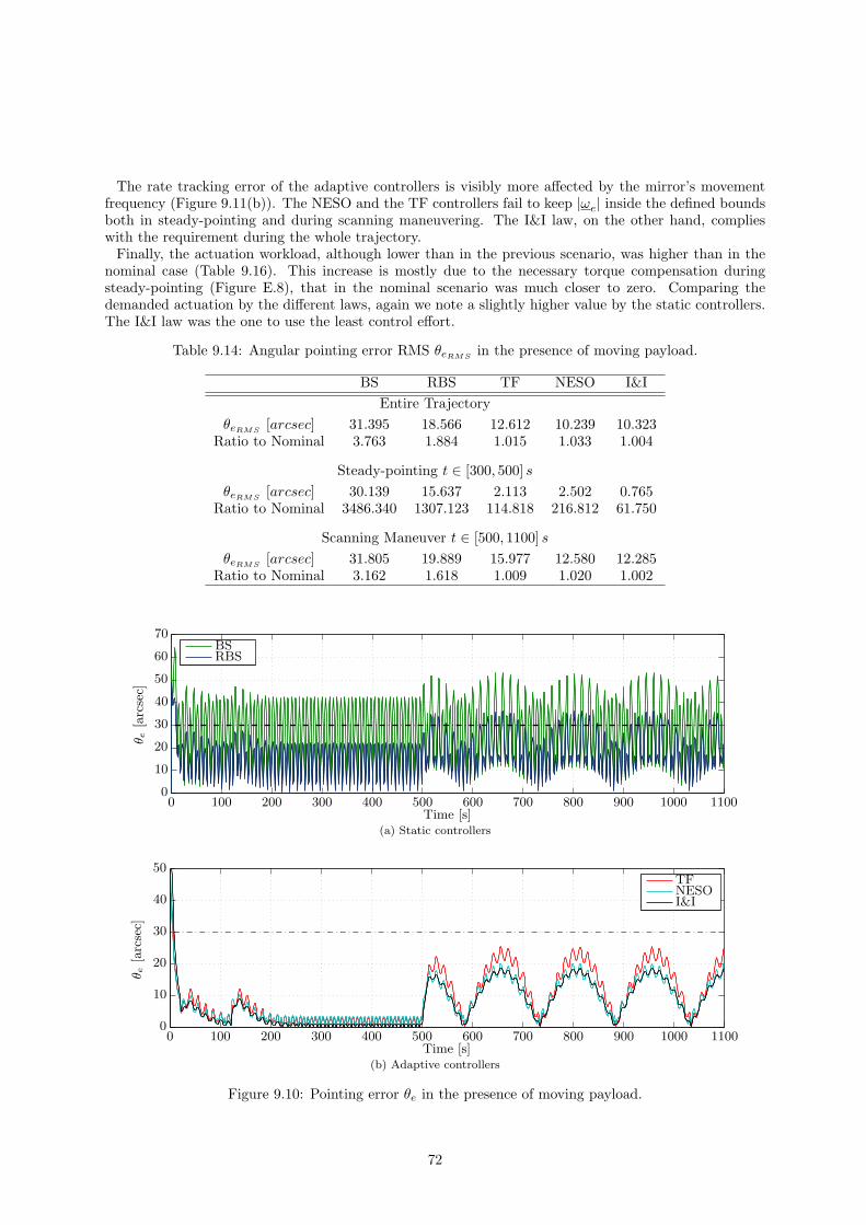
The rate tracking error of the adaptive controllers is visibly more affected by the mirror’s movementfrequency (Figure 9.11(b)). The NESO and the TF controllers fail to keep |ωe| inside the defined boundsboth in steady-pointing and during scanning maneuvering. The I&I law, on the other hand, complieswith the requirement during the whole trajectory.Finally, the actuation workload, although lower than in the previous scenario, was higher than in the
nominal case (Table 9.16). This increase is mostly due to the necessary torque compensation duringsteady-pointing (Figure E.8), that in the nominal scenario was much closer to zero. Comparing thedemanded actuation by the different laws, again we note a slightly higher value by the static controllers.The I&I law was the one to use the least control effort.
Table 9.14: Angular pointing error RMS θeRMSin the presence of moving payload.
BS RBS TF NESO I&I
Entire Trajectory
θeRMS[arcsec] 31.395 18.566 12.612 10.239 10.323
Ratio to Nominal 3.763 1.884 1.015 1.033 1.004
Steady-pointing t ∈ [300, 500] s
θeRMS[arcsec] 30.139 15.637 2.113 2.502 0.765
Ratio to Nominal 3486.340 1307.123 114.818 216.812 61.750
Scanning Maneuver t ∈ [500, 1100] s
θeRMS[arcsec] 31.805 19.889 15.977 12.580 12.285
Ratio to Nominal 3.162 1.618 1.009 1.020 1.002
RBSBS
θe[arcsec]
Time [s]0 100 200 300 400 500 600 700 800 900 1000 1100
0
10
20
30
40
50
60
70
(a) Static controllers
I&INESOTF
θe[arcsec]
Time [s]0 100 200 300 400 500 600 700 800 900 1000 1100
0
10
20
30
40
50
(b) Adaptive controllers
Figure 9.10: Pointing error θe in the presence of moving payload.
72

RBSBS
|ωe|[arcsec/s]
Time [s]0 100 200 300 400 500 600 700 800 900 1000 11000
5
10
15
20
25
(a) Static controllers
I&INESOTF
|ωe|[arcsec/s]
Time [s]0 100 200 300 400 500 600 700 800 900 1000 11000
1
2
3
4
5
(b) Adaptive controllers
Figure 9.11: Rate error norm in the presence of moving payload.
Table 9.15: Estimation error RMS during scanning motion for t ∈ [505, 1100] s in the presence of movingpayload.
TF NESO I&I
TdRMS[µNm] 26.939 23.919 8.826
Ratio to TdRMS0.172 0.152 0.056
Table 9.16: Workload along the entire trajectory in the presence of moving payload.
BS RBS TF NESO I&I
W [mJ ] 1.671 1.664 1.661 1.661 1.656
9.3.5 Influence of the Sampling Time
All deduced adaptive laws use integration steps for the computation of the disturbance estimate. Thisfact makes their performance especially dependent on the frequency at which the control law is imple-mented. So far, this frequency has been 10Hz. How would the performance of the designed controllers(static and adaptive) be if the frequency was different?To assess such influence, the simulations of the two last scenarios (uncontrolled reaction wheel and
moving payload) were repeated for all controllers at frequencies of 5, 20 and 50Hz. These scenarios werehere selected for being the most aggressive in terms of disturbance magnitude and disturbance frequency,respectively. The error RMS from these simulations is presented in Tables 9.17 and 9.18, while Table 9.19displays the ratio of estimation error RMS to the total disturbance RMS for both scenarios, during thescanning motion.The NESO and I&I controlled systems diverged for the 5Hz frequency due to high estimation gains.
To still show the performance of these controllers at the referred frequency, their estimation gains werereduced to
γ = 25 , (9.21)
73

for the I&I and
β2 = BJ0 , B =
2 0 00 2 00 0 2
, (9.22)
for the NESO, having the other parameters of this observer remained unchanged. Note that altering theestimator gains did not change the target dynamics of the referred controlled systems and, therefore,their nominal performance. The new gains were only applied to the simulations at 5Hz.As expected, the general trend is the improvement of performance with the increase of frequency and
the opposite for the decrease. It is clear the larger variation of results of the adaptive laws in bothscenarios, proving the hypothesis of higher dependence of the adaptive schemes on the implementationsampling time. In fact, in the presence of a saturated RW, the performances of the static controllers showonly insignificant changes (in the order of tenths of a percent). Only in the presence of a moving payloadthe static laws display a considerable change of error RMS, although it is always smaller than in theadaptive schemes. In this scenario the robust backstepping design (RBS) shows a higher sensitivity tothe simulation frequency than the standard design (BS). The steady-pointing performance of the staticlaws is approximately constant in both disturbance scenarios.
Table 9.17: Angular pointing error RMS θeRMS[arcsec] in the presence of a saturated RW for different
simulation frequencies. Ratio to RMS value at 10Hz shown in brackets.
f BS RBS TF NESO I&I
Entire Trajectory
5Hz 1778.083(1.000)
1095.681(1.001)
25.641(1.652)
24.794∗(2.068)
19.856∗(1.824)
20Hz 1776.788(1.000)
1094.541(1.000)
11.738(0.756)
8.839(0.737)
7.223(0.663)
50Hz 1776.792(1.000)
1094.500(1.000)
10.560(0.681)
7.798(0.650)
5.817(0.534)
Steady-pointing t ∈ [300, 500] s
5Hz 396.412(0.997)
245.333(0.997)
0.039(1.638)
0.032∗(2.143)
0.026∗(2.037)
20Hz 396.397(0.997)
245.325(0.997)
0.017(0.723)
0.010(0.697)
0.008(0.593)
50Hz 397.508(1.000)
246.013(1.000)
0.015(0.629)
0.009(0.577)
0.005(0.375)
Scanning Maneuver t ∈ [500, 1100] s
5Hz 2358.317(1.000)
1453.387(1.000)
33.972(1.695)
32.814∗(2.161)
26.279∗(2.000)
20Hz 2357.462(1.000)
1452.454(1.000)
14.628(0.730)
10.390(0.684)
7.467(0.568)
50Hz 2357.492(1.000)
1452.416(1.000)
12.703(0.634)
8.448(0.556)
4.655(0.354)
Looking now at the error from the adaptive controllers, one can see that the performance (ratio)evolution in the presence of a saturated RW for different f is similar in both trajectory stages (steady-pointing and scanning). In the case of moving payload the major changes in performance happen duringthe sinusoidal maneuver. The estimation error from the three adaptive laws, computed during thismaneuver in both scenarios, shows that only TF and NESO reduce their error with the increase offrequency. From these two, the NESO is clearly the most sensitive to the estimation sampling time,having an error decrease of about 22% for 50Hz in the two disturbance situations. Such sensitivity arisesfrom the higher order, and thus higher number of integrations, of the extended state observer. The I&Iestimator, on the other hand, is unaffected by the increase of frequency. Hence, the improvements of
∗ The designed controller diverged. Result obtained with a different estimation gain.
74

Table 9.18: Angular pointing error RMS θeRMS[arcsec] in the presence of moving payload for different
simulation frequencies. Ratio to RMS value at 10Hz shown in brackets.
f BS RBS TF NESO I&I
Entire Trajectory
5Hz 34.098(1.086)
24.394(1.314)
23.993(1.902)
19.539∗(1.908)
18.588∗(1.801)
20Hz 30.669(0.977)
16.874(0.909)
7.502(0.595)
6.548(0.640)
6.542(0.634)
50Hz 30.461(0.970)
16.431(0.885)
5.463(0.433)
5.218(0.510)
5.066(0.491)
Steady-pointing t ∈ [300, 500] s
5Hz 30.486(1.012)
15.750(1.007)
2.095(0.991)
5.860∗(2.342)
1.499∗(1.959)
20Hz 30.020(0.996)
15.606(0.998)
2.116(1.001)
2.158(0.863)
0.767(1.003)
50Hz 29.948(0.994)
15.588(0.997)
2.118(1.002)
1.954(0.781)
0.768(1.004)
Scanning Maneuver t ∈ [500, 1100] s
5Hz 36.544(1.149)
29.252(1.471)
31.738(1.986)
25.360∗(2.016)
24.568∗(2.000)
20Hz 30.490(0.959)
16.798(0.845)
8.198(0.513)
6.531(0.519)
6.180(0.503)
50Hz 30.079(0.946)
15.823(0.796)
3.810(0.238)
3.144(0.250)
2.570(0.209)
Table 9.19: Estimation error RMS ratio to total disturbance RMS (TdRMS/TdRMS
) for t ∈ [505, 1100] s atseveral frequencies in both scenarios. Ratio to the value at 10Hz in brackets.
Saturated RW Moving Payload
f TF NESO I&I TF NESO I&I
5Hz 0.012(1.146)
0.017∗(2.333)
0.006∗(2.033)
0.234(1.364)
0.366∗(2.398)
0.122∗(2.160)
20Hz 0.010(0.932)
0.006(0.861)
0.003(1.000)
0.152(0.884)
0.131(0.859)
0.056(1.000)
50Hz 0.009(0.913)
0.006(0.778)
0.003(1.000)
0.146(0.849)
0.118(0.775)
0.056(1.000)
tracking performance of this control law are only due to the better performance of the target dynamicswith a higher f . At 5Hz the NESO and I&I still generally show the best performances of all fivecontrollers, although having had an estimator gain reduction. A different way of having the NESOless sensitive to the controller’s frequency, and thus working better at low frequencies, is by letting theestimator iterate multiple times per control iteration. This attenuates the violent effect of the highestimation gains by improving the integration accuracy. Of course, this is only possible if there is enoughcomputing capacity available, even more since this observer has twice the number of states of the otheradaptation laws.
9.4 Summary of Results
In this section a brief summary of the main results of the tested scenarios is presented.
• In the disturbance-free scenario the standard backstepping (BS) proved to be the design with theleast pointing error. The robust backstepping law (RBS), due to a shift of the close-loop polescaused by the introduction of the nonlinear damping term, has a slightly slower angular trackingand, therefore, a larger error. The modular adaptive (NESO) and the immersion and invariance
75

(I&I) backstepping designs are able to achieve a performance close to the target dynamics, which isthe same as the RBS. The tuning functions adaptive backstepping controller (TF) displays the worsttracking behavior, confirming that, when tune this Lyapunov based design, fast adaptation coststracking performance. All control laws complied with the error requirements, using very similarcontrol workload.
• The introduction of a constant inertial mismatch resulted in a considerable increase in the errorof the static control laws. The RBS, for the robustness terms and contrarily to the nominal case,achieved a better performance than the BS controller. The adaptive controllers all maintained theirnominal tracking performance in all stages of the trajectory, showing the benefits of adaptation.The I&I and NESO identifiers displayed a much better disturbance estimation than the one fromTF. The error magnitude bounds were only met by the adaptive designs. The actuation workloadwas approximately the same as in the nominal case.
• The disturbance caused by a saturated reaction wheel proved to be the most demanding in termsof magnitude. Here, the error curves from the static laws reached as high as about a unit ofdegree, which is unbearably large. The adaptive designs, on the other hand and thanks to a closedisturbance estimation, only lost a small fraction of their nominal performance. Among thesedynamic feedback laws, the I&I was the one to stay closer to the disturbance-free behavior. Onlythe adaptive controllers complied with the pointing error requirements. As for the pointing stabilitybound, just the I&I was able to meet it. The adaptive laws used slightly less control workload.
• The main challenge posed by the moving payload scenario was the relatively high frequency of thedisturbance. In this situation, although the maximum tracking error of the static controllers wasonly a notch higher than the desired limit, the high frequency content of the signal caused the rateerror to oscillate completely out of the defined bound. The adaptive laws, again, maintained theoverall performance close to the nominal one. However, the steady-pointing error grew considerablyrelatively to the disturbance-free scenario. In terms of estimation, the I&I observer outperformed theremaining two identifiers. Once again, the adaptive designs managed to keep the error magnitudebelow the limit, although only the immersion and invariance law was able to steer the spacecraftinside the rate error bound. The adaptive designs, like in the previous case, used slightly lessworkload than the static laws. The I&I used the least control effort.
• The simulation of the last two scenarios using different control implementation frequencies revealedthat the adaptive performances, unlike the static ones, depend considerably on the sampling time.Among the tested estimators, the one of the NESO emerged as the most sensitive to changes in ∆t,as it has twice the number of integration steps of the other estimators. The I&I, on the other hand,displayed no significant estimation changes with the increase of simulation frequency. However,the tracking performance of this control law was the one to improve the most in both scenarios(in percentage). This happens because the estimation error of this law is the lowest of the threefor all frequencies, making the variation of performance of the target dynamics alone represent abigger slice of the overall performance. Due to the high estimation gains, the NESO and I&I lawsdiverged for f = 5Hz. A reduction of gain was enough to solve the numerical problem. Despitesuch reduction, these controllers outperformed the remaining ones at the referred frequency.
• The saturation limits defined for the command filters were not achieved during any of the performedsimulations.
76

Chapter 10
Conclusions and Recommendations
The final conclusions of the research described in this dissertation are summarized in this chap-ter. A set of recommendations and related future work possibilities are also presented.
10.1 Final Conclusions
The research presented in this dissertation focused on the robust and adaptive nonlinear attitude controlfor precise maneuvering of a rigid-body spacecraft model in terms of Modified Rodrigues Parametersperturbed by a set of different inertial-related disturbance torques. Such perturbation sources includeda constant mismatch in the inertia tensor, a faulty saturated reaction wheel and a moving spectrometermirror in the spacecraft’s payload. A survey of control designs and adaptive schemes for nonlinear systemsresulted in the selection of Backstepping, for its versatility and strong stability basis, as the base controldesign for the robust and adaptive attitude control laws.From the work described in this dissertation several conclusions can be draw, namely:
• In Chapter 7, it was possible to prove the convergence of the tuning function estimation to the truevalue of an additive unknown parameter (constant regressor), both for constant and time-variantuncertainty. In the same chapter, the immersion and invariance backstepping control law, which inthe literature is typically applied to systems with constant unknown parameters, was proved to beinput-to-state stable in the presence of time-variant uncertainties under certain circumstances.
• During the gain selection process, in Chapter 8, the tuning functions based law (TF) turned outto be very difficult to tune, being the choice of estimation gain a trade-off between fast identifierconvergence and good transient performance. The immersion and invariance controller (I&I), onthe other hand, emerged as the easiest to tune among the designed adaptive controllers. Because itis composed of two cascade interconnected stable systems, the increase of estimation gain not onlyspeeds up the update law but also considerably improves the system’s tracking performance.
• From the simulations run in a disturbance-free scenario, in Chapter 9, all controllers showed closeperformances, being the standard backstepping controller the one to have the lowest tracking errorand the TF law the one to have the highest. The remaining adaptive controllers succeeded toachieve the target dynamics behavior, which was similar to the one of the robust backsteppingcontrol law (RBS). All controlled systems met the pointing accuracy and stability requirements.
• Among the tested perturbations, the ones caused by a saturated reaction wheel and by a movingpayload mirror proved to be the most challenging for the control systems, one for its high magnitudeand the other for its relatively high frequency, respectively.
• The static control laws failed to keep both the pointing error and rate tracking error below therequirements in all disturbance scenarios. The adaptive schemes, on the contrary, proving thebenefit of dynamic feedback, succeeded to maintain a consistent behavior, having lost only a smallfraction of their nominal angular tracking performance before all tested perturbations. The pointingerror from these controllers was in all scenarios lower than the required. As for the pointing stabilitycriterion, only the I&I was able to meet it for all considered disturbances. The remaining adaptivelaws did not comply with such criterion for the two most aggressive perturbations.
• In terms of estimation, the I&I and the modular adaptive backstepping (NESO) identifiers showed agreat improvement over the much simpler tuning function estimator. However, the NESO denoted
77

the largest loss of estimation performance with the increase of disturbance frequency. The I&Idisplayed the best estimation capabilities in all perturbed scenarios.
• Although the workload used by all systems was similar for each scenario, it was possible to noticea slightly lower actuation effort required by the adaptive schemes in the two most challengingdisturbance cases. This is a direct consequence of lower tracking error.
• Having all controlled systems been run at different sampling times in the presence of the twomost aggressive perturbations, the results showed a generalized improve of performance with theincrease of implementation frequency. The improvement was much more evident for the adaptivecontrollers, proving the expected higher dependence of these laws on such simulation parameter.This dependence along with high estimation gain, made the NESO and I&I laws diverge for afrequency lower than the initially used. The reduction of the estimation gain allowed convergenceof both controllers at such frequency. The NESO identifier emerged as the most sensitive to ∆t.
• Among the designed controllers the I&I and NESO were by far the best in all scenarios. However, theI&I was the one to display the most consistent performance. The estimator design with prescribedclose-loop dynamics by system restriction to an invariant manifold, forming an easy-to-tune cascadeinterconnection of two stable systems, not only yielded the best attitude tracking before all testedperturbations but also outperformed the remaining controllers for all tested frequencies. Anothermajor advantage of this design is its input-to-state stability property with respect to the disturbancederivative, rather than to the estimation error, avoiding the need for projection operator.
10.2 Recommendations
Quite conclusive results were obtained, however, the present research can be further refined by investi-gating aspects not covered in this dissertation.
• For further simulation of the current control designs, the control allocation problem should beconsidered. In (Bakker, 2009) this topic was treated by including the dynamics of reaction wheelsand a pseudo-inverse allocation strategy. This subject could be taken to an even higher level byconsidering the RW’s motor dynamics and by performing the allocation with a more sophisticatedalgorithm that allows the assignment of actuator magnitude and rate constraints. Such algorithmcan be a quadratic programming scheme like the one described in (Harkegard, 2004). If thisapproach is followed, a possible optimization cost function could include the working principle of areaction wheel (Schaub & Junkins, 2002): the larger the rotation rate of the flywheel the more powernecessary to produce a required torque. Actuation time-delay can be treated as an uncertainty bythe adaptive backstepping controller as it is described in (Bresch-Pietri, Chauvin, & Petit, 2011).
• The tests described in this report did not include measurement noise. Not only should the simulationinclude such feature, but also the controllers should be designed taking it into account. StochasticLyapunov analysis can be a useful tool to derive a control law stable in probability as described in(Deng & Krstic, 1997) for a static backstepping law and in (Wu, Xie, & Zhang, 2007) for an adaptivebackstepping one. A possible way to strengthen the adaptive laws driven by tracking error againstmeasurement noise is to add dead-zones (Ioannou & Sun, 1996). This turns the adaptation off in asmall region around the origin, avoiding erratic estimator behavior due to noise amplification.
• The performed control design and analysis concerned only the most precision-demanding operationmode, used for scientific data acquisition. However, in order to obtain a more complete attitudecontrol system, that can be used during the entire FAST mission, the remaining mission modesshould be considered. For obvious reasons this extension might require the definition of severalgains according to the operating mode and even, for detumbling mode control, the suppressionof the angular control loop to perform angular rate regulation. This type of controller can beeasily designed by linear angular rate feedback with adaptive disturbance rejection, making use ofLyapunov stability arguments concerning the Coriolis term of the dynamics equation and treatingthe small gravity gradient induced torque as a disturbance.
• Although very aggressive disturbances were modeled to test the designed control laws, furthertesting in the presence of environmental disturbances is recommended. These can include inducedmagnetic torque, aerodynamic torque and solar radiation torque (Larson & Wertz, 2005). Thelast two, however, should have especially low magnitudes due to the quasi-cubical geometry of thespacecraft.
78

Bibliography
Adams, D., Bruno, D., Shah, P., & Keller, B. (1998). Precision Control, Knowledge and Orbit Determi-nation on a Small Spacecraft Bus: The OrbView-4 Attitude Control System. In 12th AIAA/USUConference on Small Satellites.
Aghili, F. (2011). Ripple Suppression of BLDC Motors With Finite Driver/Amplifer Bandwidth at HighVelocity. IEEE Transactions on Control Systems Technology , 19 (2), 391-397.
Artstein, Z. (1983). Stabilization with Relaxed Controls. Nonlinear Analysis , 7 , 1163-1173.Ascher, U. M., & Petzold, L. R. (1998). Computer Methods for Ordinary Differential Equations and
Differential-Algebraic Equations. SIAM.Astolfi, A., Karagiannis, D., & Ortega, R. (2008). Nonlinear and Adaptive Control with Applications.
Springer-Verlag.Astolfi, A., & Ortega, R. (2001). Immersion and Invariance: A New Tool for Stabilization and Adaptive
Control of Nonlinear Systems. In IFAC Symposium on Nonlinear Control System Design.Bakker, G. (2009). A Fault-tolerant Nonlinear Spacecraft ADCS Design in terms of Modified Rodrigues
Parameters. Unpublished master’s thesis, Delft University of Technology.Beer, F. P., Johnston, E. R., & Eisenberg, E. R. (2004). Vector Mechanics for Engineers: Statics (7th
ed.). McGraw-Hill.Blanchini, F. (2009). Lyapunov Methods in Robustness. An Introduction - Lecture notes in Automatic
Control. (Dipartimento di Matematica e Informatica, Universita di Udine, Italy)Bresch-Pietri, D., Chauvin, J., & Petit, N. (2011). Adaptive Backstepping for Uncertain Systems With
Time-Delay On-Line Update Laws. In American Control Conference.Coxeter, H. S. M. (1969). Introduction to Geometry (Second ed.). John Wiley & Sons.Deng, H., & Krstic, M. (1997). Stochastic Nonlinear Stabilization- I: A backstepping Design. Systems &
Control Letters , 32 , 143-150.Dungate, D. G. (1993). ESA Pointing Error Handbook. ESTEC, ESA-NCR-502, Issue 1.Farrell, J. A., Polycarpou, M., & Sharma, M. (2003). Adaptive Backstepping with Magnitude, Rate,
and Bandwidth Constraints: Aircraft Longitude Control. In Proceedings of the Annual AmericanControl Conference.
Farrell, J. A., Polycarpou, M., & Sharma, M. (2004). On-Line Approximation Based Control of UncertainNonlinear Systems with Magnitude, Rate and Bandwidth Constraints on the States and Actuators.In Proceeding of the 2004 American Control Conference.
Farrell, J. A., Polycarpou, M., & Sharma, M. (2005). Backstepping Based Flight Control with AdaptiveFunction Approximation. Journal of Guidance, Control and Dynamics , 28 , 1089-1102.
Farrell, J. A., Polycarpou, M., Sharma, M., & Dong, W. (2009). Command Filtered Backstepping. IEEETransactions on Automatic Control , 54 , 1391-1395.
Fujimoto, K., Yokoyama, M., & Tanabe, Y. (2010). I&I-based Adaptive Control of a Four-rotor MiniHelicopter. In 36th Annual Conference on IEEE Industrial Electronics Society.
Ge, S. S., & Wang, J. (2002). Robust Adaptive Stabilization for Time Varying Uncertain NonlinearSystems with Unknown Control Coefficients. In 41st IEEE Conrerenee on Deeision and Control.
Gill, E., Maessen, D., Laan, E., Kraft, S., & Zheng, G. T. (2010). Atmospheric Aerosol Characterizationwith the Dutch-Chinese FAST Formation Flying Mission. Acta Astronautica, 66 , 1044-1051.
Goldstein, H., Poole, C., & Safko, J. (2002). Classical Mechanics. Addison Wesley.Grotens, R. (2010). Fault Tolerant Control with Sliding Modes and Control Allocation. Unpublished
master’s thesis, Delft University of Technology.Guo, J., Maessen, D., Gill, E., Moon, S., & Zheng, G. T. (2009). Status of the FAST Mission: Micro-
Satellite Formation Flying for Technology, Science and Education. In 60th International Astronau-tical Congress.
Han, J. (1995). A Class of Extended State Observers for Uncertain Systems. Control and Decision,10 (1), 85-88. (In Chinese)
79
Han, J. (2009). From PID to Active Disturbance Rejection Control. IEEE Transactions on IndustrialElectronics , 56 (3), 900-906.
Hanson, A. J. (2006). Visualizing Quaternions (T. Cox, Ed.). Morgan Kaufmann - Elsevier.Harkegard, O. (2004). Dynamic Control Allocation Using Constrained Quadratic Programming. Journal
of Guidance, Control and Dynamics , 276 , 1028-1034.Huang, Y., & Han, J. (2000). Analysis and Design for the Second Order Nonlinear Continuous Extended
States Observer. Chinese Science Bulletin, 45 , 1938-1944.Ioannou, P., & Sun, J. (1996). Robust Adaptive Control. Prentice Hall.Isidori, A. (1995). Nonlinear Control Systems (Third ed.). Springer.Jørgensen, J. L., Denver, T., Betto, M., & Jørgensen, P. S. (2003). Microasc a Miniature Star Tracker.
In Small Satellites for Earth Observations, 4th International Symposium of the IAA.Juang, J. (2004). Instrument Attitude Precision Control (Tech. Rep.). Langley Research Center, Virginia:
NASA.Junkins, J. L., & Singla, P. (2004). How Nonlinear Is It? A Tutorial on Nonlinearity of Orbit and
Attitude Dynamics. Journal of Astronautical Sciences , 52 , 7-60.Karagiannis, D., & Astolfi, A. (2005). Nonlinear Observer Design Using Invariant Manifolds and Appli-
cations. In 44th IEEE Conference on Decision and Control.Karagiannis, D., & Astolfi, A. (2008). Nonlinear adaptive control of systems in feedback form: An
alternative to adaptive Backstepping. Systems & Control Letters , 57 , 733-739.Karagiannis, D., Astolfi, A., & Ortega, R. (2002). Adaptive Output Feedback Stabilization of a Class of
Nonlinear Systems. In 41st IEEE Conference on Decision and Cootrol.Karagiannis, D., Carnevale, D., & Astolfi, A. (2007). Output Feedback Stabilisation of a Class of Non-
linear Systems via Reduced-order Observers and Certainty Equivalence. In 46th IEEE Conferenceon Decision and Control.
Karagiannis, D., Jiang, Z. P., Ortega, R., & Astolfi, A. (2004). Output Feedback Stabilization of a Classof Uncertain Nonlinear Systems. In American Control Conference.
Khalil, H. K. (1996). Adaptive Output Feedback Control olf Nonlinear Systems Represented by Input-Output Models. IEEE Transactions on Automatic Control , 41 , 177-188.
Khalil, H. K. (2002). Nonlinear Systems (Third ed.). Prentice Hall.Kokotovic, P., & Arcak, M. (2001). Constructive Nonlinear Control: A Historical Perspective. Autimatica,
37 , 637-662.Kristiansen, R., & Nicklasson, P. J. (2005). Satellite attitude control by quaternion-based backstepping.
In Proceedings of the American Control Conference (Vol. 2, p. 907 - 912).Krstic, M., Kanellakopoulos, I., & Kokotovic, P. V. (1995). Nonlinear and Adaptive Control Design.
Wiley-Interscience.Laan, E. (2009). The Spectropolarimeter for Planetary Exploration - SPEX. Presentation at the
NVR/VSV Symposium on Small Satellites, Delft, The Netherlands.Larson, W. J., & Wertz, J. R. (2005). Space Mission Analysis and Design (Third ed.). Microcosm Press
and Kluwer Academic Publishers.Li, C., & Ma, G. (2007). Adaptive Backstepping Control for Attitude Tracking of a Spacecraft. In IEEE
International Symposium on Industrial Electronics.Luenberger, D. (1966). Observers for Multivariable Systems. IEEE Transactions on Automatic Control ,
11 (2), 190-197.Maessen, D., Guo, J., Gill, E., Gunter, B., Chu, Q. P., Bakker, G., et al. (2009). Conceptual Design
of the FAST-D Formation Flying Spacecraft. In 7th IAA Symposium on Small Satellites for EarthObservation.
Maessen, D., Guo, J., Gill, E., Laan, E., Moon, S., & Zheng, G. T. (2009). Mission Design of theDutch-Chinese FAST Micro-Satellite Mission. In 7th IAA Symposium on Small Satellites for EarthObservation.
Maessen, D., & Laan, E. (2008). Formation Flying Orbital Geometry of the Dutch-Chinese Chinese FASTMicro FAST Micro-Satellite Satellite Mission Mission. Presentation at Astrocon V Conference.
Moon, S., Hannemann, S., Bentley, M. S., Kraft, S., Wielinga, K., Kroesbergen, E., et al. (2008). AMiniaturized Laser Altimeter and Stereo Camera for a Microsatellite Formation Mission. In SmallSatellites Systems and Services (4S) Symposium.
Murugesan, S. (1981). An Overview of Electric Motors for Space Applications. IEEE Transactions onIndustrial Electronics and Control Instrumentation, IECI-28 (4), 260-265.
Nijmeijer, H., & Schaft, A. van der. (1990). Nonlinear Dynamical Control Systems. Springer-Verlag.Pomet, J., & Praly, L. (1992). Adaptive Nonlinear Regulation: Estimation from the Lyapunov Equation.
IEEE Transactions on Automatic Control , 37 , 729-740.
80

Radice, G., & Casasco, M. (2007). On Different Parameterisation Methods to Analyse Spacecraft AttitudeManoeuvres in the Presence of Attitude Constraints. The Aeronautical Journal , 111 , 335-342.
Reale, G., Ortner, P., & del Re, L. (2009). Nonlinear Observers for Closed-Loop Control of a CombustionEngine Test Bench. In American Control Conference.
Ren, Z., Wang, W., & Shen, Z. (2011). New Robust Fault-tolerant Controller for Self-repairing FlightControl Systems. Journal of Systems Engineering and Electronics , 22 (1), 77-82.
Robertson, B., & Stoneking, E. (2003). Satellite GN&C Anomaly Trends. In 26th Annual AAS Guidanceand Control Conference.
Rugh, W. J., & Shamma, J. S. (2000). Research on Gain Scheduling. Automatica, 36 , 1401-1425.Ruocchio, C., Accardo, D., Rufino, G., Mattei, S., & Moccia, A. (1999). Development and Testing of
a Fully Autonomous Star Tracker. In Digest of the 2nd International Symposium of the IAA onSmall Satellites for Earth Observation.
Sastry, S., & Bodson, M. (1989). Adaptive Control, Stability, Convergence, and Robustness (T. Kailath,Ed.). Prentice Hall.
Schaub, H., & Junkins, J. L. (1996). Stereographic Orientation Parameters for Attitude Dynamics: AGeneralization of the Rodrigues Parameters. Journal of the Astronautical Sciences , 44 , 1-19.
Schaub, H., & Junkins, J. L. (2002). Analytical Mechanics of Aerospace Systems. AIAA.Schaub, H., Tsiotras, P., & Junkins, J. L. (1995). Principal Rotation Representations of Proper NxN
Orthogonal Matrices. International Journal of Engineering Science, 33 (15), 2277-2295.Shuster, M. D. (1993). A Survey of Attitude Representations. The Journal of Astronautical Sciences ,
41 (4), 439-517.Sieberling, S., Chu, Q. P., & Mulder, J. A. (2010). Robust Flight Control Using Incremental Nonlin-
ear Dynamic Inversion and Angular Acceleration Prediction. Journal of Guidance, Control andDynamics , 33 (6), 1732-1742.
Slotine, J. E., & Li, W. (1991). Applied Nonlinear Control (First ed.). Prentice Hall.Sonneveldt, L. (2010). Adaptive Backstepping Flight Control for Modern Fighter Aircraft. Unpublished
doctoral dissertation, Delf University of Technology.Sonneveldt, L., van Oort, E., Chu, Q. P., & Mulder, J. A. (2010). Immersion and Invariance Based
Nonlinear Adaptive Flight Control. In AIAA Guidance, Navigation and Control Conference andExhibit.
Sun, D. (2007). Comments on Active Disturbance Rejection Control. IEEE Transactions on IndustrialElectronics , 54 (6), 3428-3429.
Tsiotras, P. (1994). New Control Laws for the Attitude Stabilization of Rigid Bodies. In IFAC Symposiumon Automatic Control in Aerospace.
van Oort, E., Sonneveldt, L., Chu, Q. P., & Mulder, J. A. (2007). Modular Adaptive Input-to-stateStable Backstepping of a Nonlinear Missile Model. In AIAA Guidance, Navigation and ControlConference and Exhibit.
van Oort, E., Sonneveldt, L., Chu, Q. P., & Mulder, J. A. (2010). Full Envelope Modular AdaptiveControl of a Fighter Aircraft using Orthogonal Least-Squares. Journal of Guidance, Navigationand Dynamics , 33 (5), 1461-1472.
Vukic, Z., Kuljaca, L., Donlagic, D., & Tesnjak, S. (2003). Nonlinear Control Systems. Marcel Dekker.Wang, W., & Gao, Z. (2003). A Comparison Study of Advanced State Observer Design Techniques. In
American Control Conference.Wang, W., Hameed, T., & Ren, Z. (2009). Extended State Observer-based Robust Fault-tolerant Con-
troller for Flight Control Surface Failures. In The Ninth International Conference on ElectronicMeasurement and Instruments.
Wedershoven, J. A. M. M. (2010). Analysis of Nonlinear Dynamic Inversion based control law designs:Application to an F-16 Model. Unpublished master’s thesis, Delft University of Technology.
Wie, B. (2008). Space Vehicle Dynamics and Control (Second ed.; J. A. Schetz, Ed.). AIAA.Wiesel, W. E. (1997). Spaceflight Dynamics (Second ed.). Irwin/McGraw-Hill.Wu, Z. J., Xie, X. J., & Zhang, S. Y. (2007). Adaptive Backstepping Controller Design Using Stochastic
Small-gain Theorem. Autimatica, 43 , 608-620.Yang, Z. (2010). An Improved Adaptive Robust Motion Controller Combined with Disturbance Observer.
In IEEE International Conference on Control Applications.Yang, Z., Hara, S., Kanae, S., Wada, K., & Su, C. (2010). An Adaptive Robust Nonlinear Motion Con-
troller Combined With Disturbance Observer. IEEE Transactions on Control Systems Technology ,18 (2), 454-462.
Yang, Z., Tsubakihara, H., Kanae, S., Wada, K., & Su, C. (2006). A Novel Robust Nonlinear MotionController with Disturbance Observer. In IEEE International Conference on Control Applications.
Yip, P. P., & Hedrick, J. K. (1998). Adaptive Dynamic Surface Control: A Simplified Algorithm for
81

Adaptive Backstepping Control of Nonlinear Systems. International Journal of Control , 71 , 959-979.
Yuan, R., Fan, G., Yi, J., & Yu, W. (2009). Robust Attitude Controller for Unmanned Aerial VehicleUsing Dynamic Inversion and Extended State Observer. In Second International Conference onIntelligent Computation Technology and Automation.
Zhang, X.-Y., & Lin, Y. (2010). A Robust Adaptive Dynamic Surface Control for Nonlinear Systemswith Hysteresis Input. Acta Automatica Sinica, 36 , 1264-1271.
Zheng, Q. (2009). On Active Disturbance Rejection Control: Stability Analysis And Applications InDisturbance Decoupling Control. Unpublished doctoral dissertation, Cleveland State University.
Zhou, J., & Wen, C. (2008). Adaptive Backstepping Control of Uncertain Systems. Springer.Zhu, Z., Xia, Y., Fu, M., & Wang, S. (2010). Attitude Tracking of Rigid Spacecraft Based on Ex-
tended State Observer. In 3rd International Symposium on Systems and Control in Aeronauticsand Astronautics (p. 621-626).
Ziemer, J. K., Cubbin, E. A., Choueiri, E. Y., Oraevsky, V., & Dokukin, V. (1996). Pulsed PlasmaPropulsion for a Small Satellite: Mission COMPASS P3OINT. In 32nd AIAA/ASME/SAE/ASEEJoint Propulsion Conference and Exhibit.
82

Appendix A
Modified Rodrigues Parameters
A.1 MRP Kinematics Derivation
In this section the MRP kinematics is obtained through the derivation of the quaternion parameterkinematics.First, to arrive at the matrix N(q), consider the Rodrigues formula in matrix form (direction cosine
matrix) written in terms of quaternions (3.17)
C(q, q4) = I − 2q4Sq + 2S2q ,
or in matrix form as
C(q, q4) =
1− 2(q22 + q23) 2(q1q2 + q3q4) 2(q1q3 − q2q4)2(q1q2 − q3q4) 1− 2(q21 + q23) 2(q2q3 + q1q4)2(q1q3 + q2q4) 2(q2q3 − q1q4) 1− 2(q21 + q22)
(A.1)
which can be replaced in Poisson’s kinematic differential equation for the direction cosine matrix (3.7)yielding
C = −SωBOC = −SωBO
(I − 2q4Sq + 2S2
q
),
The diagonal elements of C are
C =
−4(q2q2 + q3q3) ∗ ∗∗ −4(q1q1 + q3q3) ∗∗ ∗ −4(q1q1 + q2q2)
Matching these elements with the diagonal entries of −SωBOC yield the system
−4(q2q2 + q3q3) = 2ωBO3 (q1q2 − q3q4)− 2ωBO
2 (q1q3 + q2q4)
−4(q1q1 + q3q3) = −2ωBO3 (q1q2 + q3q4) + 2ωBO
1 (q2q3 − q1q4)
−4(q1q1 + q2q2) = 2ωBO2 (q1q3 − q2q4)− 2ωBO
1 (q2q3 + q1q4)
which, arranged into matrix form gives
0 q2 q3q1 0 q3q1 q2 0
q1q2q3
=1
2
0 (q1q3 + q2q4) −(q1q2 − q3q4)−(q2q3 − q1q4) 0 (q1q2 + q3q4)(q2q3 + q1q4) −(q1q3 − q2q4) 0
ω1
ω2
ω3
BO
This system can be solved for[q1 q2 q3
]Tresulting in
q1q2q3
=1
2
q4 −q3 q2q3 q4 −q1−q2 q1 q4
ω1
ω2
ω3
BO
=1
2(Sq + q4 I)ω
BO
To obtain the time derivative of the forth quaternion we take the time-derivative of the Holonomicconstraint
d
dt
(q24 + qT q
)= 2q4q4 + 2qT ˙q = 0
q4 = − 1
q4qT ˙q = − 1
2q4qT (Sq + q4 I)ω
BO = −1
2qTωBO
83

It is now possible to write the kinematics equation for the four quaternion parameters in the form of(3.1)
[˙qq4
]
=1
2
[Sq + q4 I−qT
]
ωBO (A.2)
Knowing that the modified Rodrigues parameters are given in terms of the quaternions parameters by(3.8)
σ =q
1 + q4(A.3)
the MRP time-derivative can be expressed as
σ =1
1 + q4˙q − q
(1 + q4)2q4 (A.4)
Replacing the quaternion kinematics (A.2) in (A.4) gives
σ =1
2
(1
1 + q4Sq +
q41 + q4
I +1
(1 + q4)2qqT
)
ωBO (A.5)
The relations
q =2σ
1 + |σ|2 , q4 =1− |σ|21 + |σ|2 (A.6)
can be replaced in (A.5) yielding the MRP kinematics
σ =1
4
[2Sσ + (1− |σ|2)I + 2σσT
]ωBO (A.7)
withωBO = ω + nc2(σ) (A.8)
A.2 MRP Algebra
In this section some quaternion operations are extended to the MRPs. These include: composition,multiplication and division.The quaternion composition operation is obtained from the multiplication of cosine direction matrices
and is defined as (Shuster, 1993)
C(q′′) = C(q′)C(q) ⇒ q′′ = q′ ⊗ q =
[q4q
′ + q′4q − q′ × qq4q
′4 − qT q′
]
(A.9)
This operation can be applied to MRP by using the identities
q =2σ
1 + |σ|2 , q4 =1− |σ|21 + |σ|2 , (A.10)
which gives
σ′′ = σ′ ⊗ σ =2σ′ + 2σ − 4Sσ′σ
(1 + |σ|2)(1 + |σ′|2) + (1− |σ|2)(1− |σ′|2)− 4σTσ′
=(1− |σ|2)σ′ + (1− |σ′|2)σ − 2Sσ′σ
1 + |σ|2|σ′|2 − 2σTσ′ (A.11)
A similar operation, the quaternion multiplication, is defined as
q′′ = q q′ ⇒ σ′′ = σ σ′ (A.12)
The composition and multiplication operations are related by σ σ′ ≡ σ′ ⊗ σ.The inverse of the quaternion multiplication, the quaternion division, is defined
q = q′′ q′ (A.13)
84

and can be related to the multiplication rule using the inverse quaternion (Shuster, 1993)
q−1 .=
[−qq4
]
(A.14)
by
q = q′′ q′ = q′′ q′−1 = q′−1 ⊗ q′′ =
[−q′′4 q
′ + q′4q′′ + q′ × q′′
q′′4 q′4 + q′′T q′
]
(A.15)
The logic used in quaternion algebra can be applied to MRPs
σ = σ′′ σ′ = σ′′ (−σ′) = (−σ′)⊗ σ′′ =(1− |σ′|2)σ′′ − (1− |σ′′|2)σ′ + 2Sσ′σ′′
1 + |σ′′|2|σ′|2 + 2σ′′Tσ′ (A.16)
A.3 MRP Error and Error Rate Derivations
The angular error in terms of Modified Rodrigues Parameters can be defined in two different ways: theMRP necessary to go from the desired attitude till the actual one, or the inverse rotation order. Here weuse the latter which is expressed by
σr = σ σe = σe ⊗ σ (A.17)
The MRP error can then be given by
σe = σr ⊗ (−σ) =(1− |σ|2)σr − (1− |σr|2)σ − 2Sσσr
1 + |σ|2|σr|2 + 2σTσr
=Num
Den(A.18)
The time-derivative of the MRP error is given by
σe =∂σe
∂σσ +
∂σe
∂σr
σr =1
Den
[(∂Num
∂σ− σe
∂Den
∂σ
)
σ +
(∂Num
∂σr
− σe
∂Den
∂σr
)
σr
]
(A.19)
where
∂Num
∂σ= −2σrσ
T − (1− |σr|2)I + 2Sσr,
∂Den
∂σ= |σr|2σT + 2σT
r , (A.20)
∂Num
∂σr
= 2σσTr + (1− |σ|2)I − 2Sσ ,
∂Den
∂σr
= |σ|2σTr + 2σT , (A.21)
A.4 Compensated MRP Tracking Error Approximation
In the framework of command filtering backstepping, the compensated tracking error is used to “hide”the true tracking error from the control algorithm in case of actuator saturation in order to avoid in-stability. This error is computed by subtracting the effect of the command filters χ (that include thesaturation limits) to the true tracking error z. In regular states this is a linear operation, however inangular representations such as quaternion parameters or MRPs this, in principle, has to be computedusing the angular error definition. In MRP algebra the true error MRP σz is equal to the “bearable” (orcompensated) error MRP σz rotated an amount equal to the “unbearable” excess error σχ
σz = σz σχ (A.22)
which inverted into division form gives
σz = σz σχ =(1− |σχ|2)σz − (1− |σz|2)σχ − 2Sσz
σχ
1 + |σz|2|σχ|2 + 2σTz σχ
(A.23)
If the reference signals are designed to be slow enough for the controllers to track them with a reasonableperformance and taking into consideration the saturation limits of actuators, then the tracking error and,simultaneously, the “unbearable” amount of error will both be small
σz 1 , σχ 1
⇒ σz ≈ σz − σχ ≡ z ≈ z − χ (A.24)
where the approximation (A.24) was obtained by neglecting all the quadratic terms.
85

Appendix B
Boundedness of the Disturbance
Torque
In the framework of robust and adaptive backstepping the property of boundedness is of the utmostimportance. As it was shown in Chapters 6 and 7, the input-to-state stability property of the robustness-added algorithms depend on the boundedness of the disturbance and sometimes even of its time-derivative.For the practical implementation, the use of command filters simplifies the robust designs by requiring,in most cases, only that the perturbation value does not grow to infinity. The exception is the Immersionand Invariance which for the proof of input-to-state stability needs boundedness of T d.In this appendix it will be proved that, for the considered scenarios, the disturbance torque and its
time-derivative are both bounded under the condition of bounded input torque and bounded state which,by the inclusion of command filters and use of MRP shadow parameter, are both satisfied.
B.1 Norm Tools
Here some mathematical tools are presented that will be used in the following sections to analyze theboundedness of the disturbance vector.The 2-norm of a vector is given by
‖v‖ =√
|v1|2 + |v2|2 + · · ·+ |vn|2 (B.1)
and satisfies the triangular inequality
‖v + w‖ ≤ ‖v‖+ ‖w‖ (B.2)
The induced 2-norm of a m× n matrix can be given by (Ioannou & Sun, 1996)
‖A‖ = sup‖v‖=1
‖Av‖ , v ∈ Rn (B.3)
and has the following properties
‖Av‖ ≤ ‖A‖‖v‖ , v ∈ Rn (B.4)
‖AB‖ ≤ ‖A‖‖B‖ (B.5)
‖A+B‖ ≤ ‖A‖+ ‖B‖ (B.6)
The cross-product operation can be expressed as
v × w = ‖v‖‖w‖ sin(θ)n , (B.7)
where θ is the angle from v to w and n is the unit vector normal to the plane containing v and w in thedirection given by the right-hand rule.Applying the 2-norm to (B.7) yields
‖v × w‖ = ‖v‖‖w‖| sin(θ)| ≤ ‖v‖‖w‖ (B.8)
Let A ∈ Rm×n and w ∈ R
n be bounded. There is a positive finite constant γ such that
‖Aw‖ ≤ ‖A‖‖w‖ ≤ γ‖w‖ (B.9)
then, using (B.8), the following inequality holds
‖v ×Aw‖ ≤ γ‖v‖‖w‖ (B.10)
86
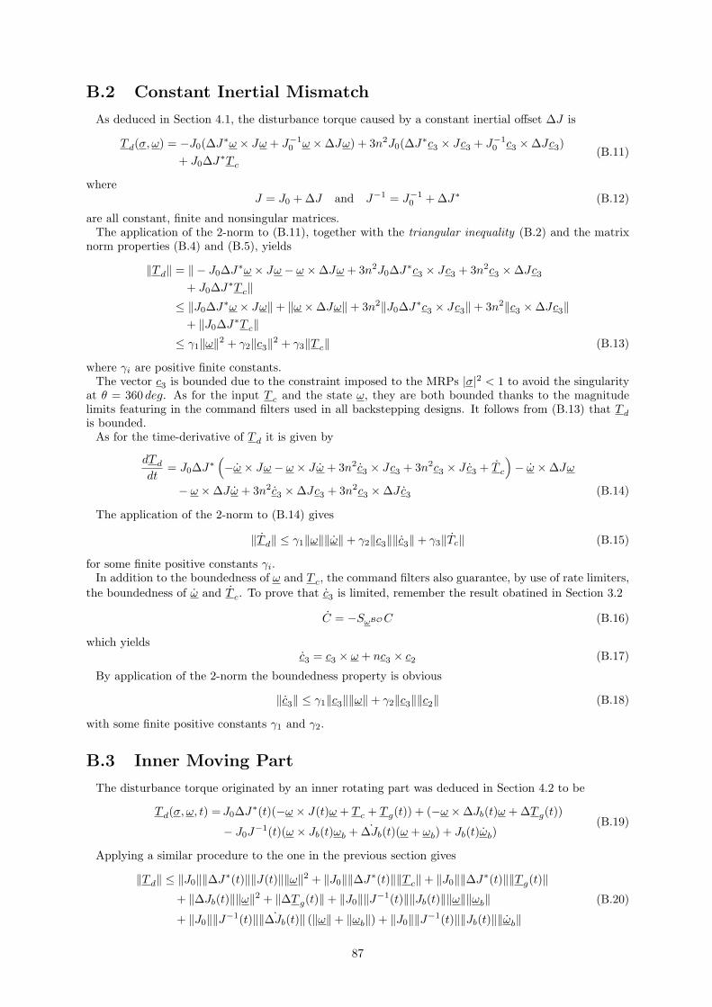
B.2 Constant Inertial Mismatch
As deduced in Section 4.1, the disturbance torque caused by a constant inertial offset ∆J is
T d(σ, ω) = −J0(∆J∗ω × Jω + J−10 ω ×∆Jω) + 3n2J0(∆J∗c3 × Jc3 + J−1
0 c3 ×∆Jc3)
+ J0∆J∗T c
(B.11)
whereJ = J0 +∆J and J−1 = J−1
0 +∆J∗ (B.12)
are all constant, finite and nonsingular matrices.The application of the 2-norm to (B.11), together with the triangular inequality (B.2) and the matrix
norm properties (B.4) and (B.5), yields
‖T d‖ = ‖ − J0∆J∗ω × Jω − ω ×∆Jω + 3n2J0∆J∗c3 × Jc3 + 3n2c3 ×∆Jc3+ J0∆J∗T c‖
≤ ‖J0∆J∗ω × Jω‖+ ‖ω ×∆Jω‖+ 3n2‖J0∆J∗c3 × Jc3‖+ 3n2‖c3 ×∆Jc3‖+ ‖J0∆J∗T c‖
≤ γ1‖ω‖2 + γ2‖c3‖2 + γ3‖T c‖ (B.13)
where γi are positive finite constants.The vector c3 is bounded due to the constraint imposed to the MRPs |σ|2 < 1 to avoid the singularity
at θ = 360 deg. As for the input T c and the state ω, they are both bounded thanks to the magnitudelimits featuring in the command filters used in all backstepping designs. It follows from (B.13) that T d
is bounded.As for the time-derivative of T d it is given by
dT d
dt= J0∆J∗
(
−ω × Jω − ω × Jω + 3n2c3 × Jc3 + 3n2c3 × Jc3 + T c
)
− ω ×∆Jω
− ω ×∆Jω + 3n2c3 ×∆Jc3 + 3n2c3 ×∆Jc3 (B.14)
The application of the 2-norm to (B.14) gives
‖T d‖ ≤ γ1‖ω‖‖ω‖+ γ2‖c3‖‖c3‖+ γ3‖Tc‖ (B.15)
for some finite positive constants γi.In addition to the boundedness of ω and T c, the command filters also guarantee, by use of rate limiters,
the boundedness of ω and T c. To prove that c3 is limited, remember the result obatined in Section 3.2
C = −SωBOC (B.16)
which yieldsc3 = c3 × ω + nc3 × c2 (B.17)
By application of the 2-norm the boundedness property is obvious
‖c3‖ ≤ γ1‖c3‖‖ω‖+ γ2‖c3‖‖c2‖ (B.18)
with some finite positive constants γ1 and γ2.
B.3 Inner Moving Part
The disturbance torque originated by an inner rotating part was deduced in Section 4.2 to be
T d(σ, ω, t) = J0∆J∗(t)(−ω × J(t)ω + T c + T g(t)) + (−ω ×∆Jb(t)ω +∆T g(t))
− J0J−1(t)(ω × Jb(t)ωb +
˙∆Jb(t)(ω + ωb) + Jb(t)ωb)(B.19)
Applying a similar procedure to the one in the previous section gives
‖T d‖ ≤ ‖J0‖‖∆J∗(t)‖‖J(t)‖‖ω‖2 + ‖J0‖‖∆J∗(t)‖‖T c‖+ ‖J0‖‖∆J∗(t)‖‖T g(t)‖+ ‖∆Jb(t)‖‖ω‖2 + ‖∆T g(t)‖+ ‖J0‖‖J−1(t)‖‖Jb(t)‖‖ω‖‖ωb‖+ ‖J0‖‖J−1(t)‖‖ ˙∆Jb(t)‖ (‖ω‖+ ‖ωb‖) + ‖J0‖‖J−1(t)‖‖Jb(t)‖‖ωb‖
(B.20)
87

with
‖∆J∗(t)T g(t)‖ = ‖∆J∗(t)(T g0+∆T g)‖ ≤ 3n2(‖∆J∗(t)c3 × J0c3‖+ ‖∆J∗(t)c3 ×∆Jb(t)c3‖)
≤ 3n2‖J0‖‖∆J∗(t)‖‖c3‖2 + 3n2‖∆J∗(t)‖‖∆Jb(t)‖‖c3‖2 ,(B.21)
Physically, an unbounded inertia implies the possibility of either infinite mass or infinite distance to therotation axis. It is then possible to conclude on the boundedness of all the inertia matrices in the studiedscenarios by Reductio ad absurdum. Their inverse is guaranteed to be bounded since, by definition, aninertia matrix is always nonsingular for a real object (with 3 non null dimensions).
As for the inertia time-derivative ˙∆Jb(t) it can be computed by
˙∆Jb(t) =d
dt
∑
mi∈b
mi
(rTi ri − rir
Ti
)=∑
mi∈b
mi
(2rTi ri − rir
Ti − rir
Ti
)
= −∑
mi∈b
mi
(Sωb
rirTi + rir
Ti Sωb
), (B.22)
considering only a rotational motion of b, i.e. ri = ωb × ri. From (B.22) it is obvious that a boundedangular velocity of the piece b, together with finite dimensions, results in a bounded time-derivative ofJb. Similar conclusions can be drawn for the consecutive derivatives of the inertia matrix by consideringboundedness the equivalent derivatives of the angular position of the part b.Using the matrix norm properties (B.4)-(B.6) the norm (B.20) becomes
‖T d‖ ≤ γ1‖ω‖2 + γ2‖T c‖+ γ3‖c3‖2 + γ4‖ω‖‖ωb‖+ γ5‖∆Jb(ωb)‖(‖ω‖+ ‖ωb‖) + γ6‖ωb‖ (B.23)
for some positive finite constants γi.Additionally to the boundedness of the states and input signal, the angular velocity and acceleration
of the part b must be bounded, also since the boundedness of the inertia time-derivative requires ωb tobe bounded. If this is satisfied T d is bounded.The time-derivative of T d is given in the case of moving inner part by
dT d
dt= J0
˙∆J∗(t)[
−ω × J(t)ω + T c + T g(t)]
+ J0∆J∗(t)
[
−ω ×(
∆Jb(t)ω + J(t)ω)
−ω × J(t)ω + Tc + Tg(t)]
− ω ×∆Jb(t)ω − ω ×(
˙∆Jb(t)ω +∆Jb(t)ω)
+ ∆T g(t)
− J0˙∆J∗(t)
[
ω × Jb(t)ω + ˙∆Jb(t)(ω + ωb) + Jb(t)ωb
]
− J0J−1(t)
[
ω × Jb(t)ω
+ω × (∆Jb(t)ω + Jb(t)ω) + ∆Jb(t)(ω + ωb) +˙∆Jb(t)(ω + ωb) + ∆Jb(t)ωb + Jb(t)ωb
]
(B.24)
where the time-derivative of the gravity induced torque is
T g = T g0+ ∆T g = 3n2
[
c3 × J0c3 + c3 × J0c3 + c3 ×∆Jb(t)c3 + c3 × (∆Jb(t)c3 +∆Jb(t)c3)]
(B.25)
The 2-norm of (B.24) can be proved to be
‖Td‖ ≤ ‖ ˙∆J∗(ωb)‖[
γ1‖ω‖2 + γ2‖T c‖+ γ3‖c3‖2 + γ4‖ωb‖+ ‖∆Jb(ωb)‖ (γ5‖ω‖+ γ6‖ωb‖)]
+ ‖∆Jb(ωb)‖(γ7‖ω‖2 + γ8‖c3‖2 + γ9‖ω‖+ γ10‖ωb‖) + γ11‖c3‖‖c3‖+ γ12‖ω‖‖ω‖+ ‖∆Jb(ωb, ωb)‖(γ13‖ω‖+ γ14‖ωb‖) + γ15‖Tc‖+ γ16‖ωb‖ (B.26)
for some positive finite constants γi.The inequality (B.26) implies that, for the disturbance’s time-derivative to be bounded, additionally
to the conditions necessary for the boundedness of T d, the time-derivative of the angular acceleration ofthe piece b must also be bounded.
88

Appendix C
Command Filter and Parameter
Projection
C.1 Command Filter
As described in Sections 6.2.3, 6.3.3, 7.3 and 7.4.4 the backstepping design can be simplified by theuse of command filters. These compute the time-derivative of the virtual control inputs as well as filterthe signal itself being able to impose magnitude and rate constraints. This appendix presents the filterdesign used for this thesis’s simulations.In (Farrell et al., 2003) the filter is given by:
[xf1
xf2
]
=
[0 10 −2ζωn
] [xf1
xf2
]
+
[0
2ζωn
]
sat
(ω2n
2ζωn
[sat(x0
c)− xf1
])
(C.1)
[xc
xc
]
=
[1 00 1
] [xf1
xf2
]
(C.2)
where x0c is the filter input signal and xf1 , xf2 are filter states. The filter can be better understood
through Figure C.1.
ω2n
2ζωn
2ζωn
Figure C.1: Command filter design with magnitude and rate limiters (Farrell et al., 2004).
When the signals are not saturated the filter (C.1) becomes:[xf1
xf2
]
=
[0 1
−ω2n −2ζωn
] [xf1
xf2
]
+
[0ω2n
]
x0c (C.3)
which is equivalent to the tranfer function:
Q(s) =ω2n
s2 + 2ζωns+ ω2n
[1s
]
(C.4)
where ζ and ωn are, respectively, the damping coefficient and the natural frequency of the filter. Thelatter has to be selected high enough so that the effect of the filter, when the signals are not saturated,is neglectable.
89

This filter philosophy can be implemented in discrete-time by using finite differences and Euler inte-gration. This is done by:
[xf1(k)xf2(k)
]
=
[1 00 0
] [xf1(k − 1)xf2(k − 1)
]
+
[∆t1
]
sat
(
sat(x0c(k)
)− xf1(k − 1)
∆t
)
(C.5)
[xc(k)xc(k)
]
=
[1 00 1
] [xf1(k)xf2(k)
]
(C.6)
The working principle of the discrete-time version is simple (see Figure C.2): the input raw signal x0c(k)
is passed through a saturation block to limit its magnitude to Mm. Then, with finite differences, theslope between sat(x0
c(k)) and xc(k − 1) is computed and its value is compared to the rate saturationlimits Mr.
k − 1 k − 1k k
xc(k − 1) xc(k − 1)
Mm
Mm
x0c(k) x0
c(k)
sat(x0c(k))
xc(k)
Mr
Mr
xc(k) = sat(x0c(k))
Figure C.2: Command filter magnitude saturated output (left plot) and rate saturated output (rightplot).
If the limiters are not in effect the filter becomes:[xf1(k)xf2(k)
]
=
[0 0
− 1∆t 0
] [xf1(k − 1)xf2(k − 1)
]
+
[11∆t
]
x0c(k) (C.7)
which yields xc(k) equal to x0c(k) and xc(k) directly computed through finite differences between x0
c(k)and xc(k − 1).The saturation operator can be defined with a hyperspherical set as:
sat(x) =
x if ‖x‖ < M
xM
‖x‖ otherwise(C.8)
or with a hypercubical set as:
sat(xi) =
xi if |xi| < Mi
sign(xi)Mi otherwise(C.9)
Implementation
Two command filters are used in the design of the adaptive control laws: one for the virtual control x2, cand one for the control input T c. The former signal is a reference for the inner loop, i.e. is an angularrate. As the integration and differentiation are defined by the frequency of the simulation (through thetime step value), the only features left to design are the saturation sets for the filtered signals and theirrates. The four sets are chosen hyperspherical and with the limits presented in Table C.1.The present dissertation focus on precise pointing control, therefore the operating envelope should be
defined so that all sensors are active and able to provide their best performance. Among the sensorsavailable the most accurate are typically the autonomous star trackers (Larson & Wertz, 2005), however,these sensors can only work properly below a certain angular rate value. In (Jørgensen, Denver, Betto,
90

Table C.1: Saturation sets limits.
Mm Mr
x2,c 1 deg/s 0.15 deg/s2
T c 0.05√
43 Nm 6Nm/s
& Jørgensen, 2003) the common star tracker requirement for maximum operating rate is |ω| < 1 deg/s.As for the maximum admissible angular acceleration the requirements vary considerably, in (Ruocchio,Accardo, Rufino, Mattei, & Moccia, 1999) it is indicated to be |ω| < 0.15 deg/s2. Higher values arecommon, nevertheless, we will take the most conservative for the sake of generality. The value for themagnitude limit of the control torque corresponds to the radius of the spherical torque envelope producedby the Tetrahedral reaction wheel configuration (Bakker, 2009). The maximum torque rate generatedby the reaction wheel set can be estimated from the bandwidth of the RW motor torque control system.In (Murugesan, 1981), the most common type of electric motor used in space reaction wheels is said tobe the (iron-less) brushless DC motor. A large size motor of this type with torque control can have, asdescribed in (Aghili, 2011), a bandwidth of 100 rad/s. Since no information was found regarding smallerscale motors of such type, and knowing that the smaller the motor the higher the bandwidth and thusthe higher torque rate produced, again for conservativeness we will take this value. The maximum torquerate was then estimated assuming a first order transfer function and taking the rounded value of theproduct of the maximum torque and the bandwidth.
C.2 Parameter Projection
In the framework of modular adaptive backstepping (Section 7.1) the property of input-to-state stabilityof the tracking error with respect to the disturbance estimation requires boundedness of the estimatedvalue. This is also required for the integrated adaptive design when the uncertainty is time-variable(Section 7.2.3). The most common way to achieve such property is by using Parameter Projection. Thismethod constrains the estimated values to a defined convex set Ω which is known to contain the trueparameter/disturbance value:
Ω = θ ∈ Rp | P(θ) ≤ 0 (C.10)
The simplest way is to stop the update law when the estimation reaches the boundary of the defined set∂Ω (Ioannou & Sun, 1996; Sastry & Bodson, 1989):
˙θ =
τ if θ ∈ Ω
τ if θ ∈ ∂Ω and θTτ ≤ 0
0 otherwise
(C.11)
where τ is the update law. This type of solution was used with success in an adaptive backstepping designwith tuning functions of a spacecraft attitude controller in (Li & Ma, 2007). However, the discontinuousnature of its definition might pose stability issues. A “smoothed” projection operator have been proposedin (Pomet & Praly, 1992) and from it many designs have been suggested. One of them, proposed in(Khalil, 1996), defines two projection operators: one based on a compact ball set and another using ona convex hypercube set.If the estimation limits are defined as a hyperspherical set around the origin, the function P(θ) can be
defined as:
P(θ) =θTθ −M2
δ(C.12)
where δ > 0 is a small constant and M is the radius of the spherical set. May us define a slightly largerset:
Ωδ = θ ∈ Rp | P(θ) ≤ 1 (C.13)
The smaller the value selected for δ the closer Ωδ will be to the originally desired set:
Ω = θ ∈ Rp | θT θ ≤ M2 (C.14)
91

In (Pomet & Praly, 1992) the “smoothed” projection is given by:
Proj (τ) =
τ if P(θ) ≤ 0
τ if P(θ) > 0 and ∇P(θ)τ ≤ 0
τ − P(θ)∇P(θ)τ
‖∇P(θ)‖2∇P(θ)T otherwise
(C.15)
where for ease of notation ∇P(θ) = ∂P(θ)
∂θ. Having defined (C.12) then (C.15) becomes:
Proj (τ) =
τ if θTθ ≤ M2
τ if θTθ > M2 and θ
Tτ ≤ 0
τ − (θTθ −M2)
δ‖θ‖2θTτ θ otherwise
(C.16)
Analyzing (C.15) one can see that, when the parameter estimation satisfies P(θ) ≤ 0 the update law is
not changed. On the other hand, when 0 < P(θ) ≤ 1 the update law is subtracted a vector perpendicular
to the boundary P(θ) = λ, resulting in a smooth update law from λ = 0, which gives τ , to λ = 1, yieldinga vector tangent the sphere. This is nothing more than “projecting” the out-of-bounds estimation to theboundary surface.
Implementation
The defined operator is to be used in the modular adaptive backstepping and in the integrated adaptivedesigns. In the former, it is applied both to the disturbance torque and angular velocity estimation laws
of the NESO, while in the latter design, since only the uncertainty is estimated, only to˙T d.
In (Bakker, 2009) the nominal torque envelope of the Tetrahedron reaction wheel configuration wasfound to be a sphere. For the projection set of the disturbance torque, is then only natural to choose aboundary close to the actuator performance limits. However, since the command filters are in use, it isnot mandatory to keep the disturbance rejection request, and thus the disturbance estimation, below theRW saturation limits. Actually, it is beneficial to maintain the estimated value correct, although it is notphysically possible for the spacecraft to reject it right away. This can be easily justified by accountingfor the effect of the command filters: even when the control actuation saturates the estimators willnot unlearn, as the signals are being compensated, making the control law always aware of the trueuncertainty values and allowing disturbance rejection as soon as control effort is available. On the otherhand, if the estimation is “blocked” by projection algorithm the controller will no longer know about thereal value of the disturbance and, when the actuators unsaturate, the estimation will still need to “catchup”.As for the projection of the angular rate, it should obey the same principle and, this way, be defined
with a slightly larger set than the chosen angular rate envelope.The projection set parameters for the two variables are then selected as shown in Table C.2.
Table C.2: Projection sets.
M δ
ω 2 deg/s 0.02 deg/s
T d 0.1Nm 0.001Nm
92
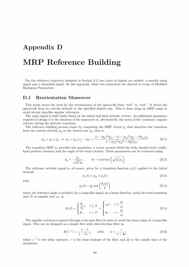
Appendix D
MRP Reference Building
For the reference trajectory designed in Section 9.2, two types of signals are needed: a smooth rampsignal and a sinusoidal signal. In this appendix, these two maneuvers are derived in terms of ModifiedRodrigues Parameters.
D.1 Reorientation Maneuver
This mode serves the need for the reorientation of the spacecraft from “rest” to “rest”. It drives thespacecraft from its current attitude to the specified desired one. This is done using an MRP ramp toavoid abrupt step-like angular references.The ramp signal is built easily based on the initial and final attitude vectors. An additional parameter
required to design it is the duration of the maneuver or, alternatively, the norm of the (constant) angularvelocity during the attitude transition.The reference building process starts by computing the MRP vector σt that describes the transition
from the current attitude σ0 to the desired one σd, that is
σd = σt ⊗ σ0 ⇒ σt = σd ⊗ (− σ0) =(1− |σ0|2)σd − (1− |σd|2)σ0 − 2Sσ
0σd
1 + |σ0|2|σd|2 + 2σT0 σd
(D.1)
The transition MRP σt provides two quantities: a vector around which the body should rotate (right-hand positive rotation) and the angle of the total rotation. These parameters can be extracted using
kt =σt
√
σTt σt
, θt = 4arctan
(√
σTt σt
)
(D.2)
The reference attitude signal is, of course, given by a transition function σt(t) applied to the initialattitude
σr(t) = σ0 σt(t) (D.3)
with
σt(t) = kt tan
(θr(t)
4
)
(D.4)
where the reference angle is modeled, for a ramp-like signal, as a linear function, using the total transitiontime Tt or angular rate ωt, as
θr(t) =
θtTt
t , t ≤ T
θt , t > T
=
ωtt , t ≤ θtωt
θt , t >θtωt
(D.5)
The angular evolution is passed through a low-pass filter in order to avoid the sharp edges of a ramp-likesignal. This can be designed as a simple first order discrete-time filter as
H(z−1) =1− λ
1− λz−1with λ =
τ
τ +∆t(D.6)
where z−1 is the delay operator, τ is the time-constant of the filter and ∆t is the sample time of thesimulation.
93

D.2 Scanning Maneuver
This maneuver drives the spacecraft in a sinusoidal manner around a fixed axis, allowing the measuringinstruments to “sweep” a certain area of the Earth’s surface, for example.The first step to design the reference signal is defining the two attitude vectors of the extremes of the
oscillations, σmax and σmin. Then, the oscillation axis and angular amplitude are extracted from thetransition MRP, computed between σmax and σmin
σt =(1− |σmin|2)σmax − (1− |σmin|2)σmax − 2Sσmin
σmax
1 + |σmin|2|σmax|2 + 2σTminσmax
(D.7)
The axis vector kr and the angle amplitude Aθ are
kr =σt
√
σTt σt
, Aθ = 4arctan
(√
σTt σt
)
(D.8)
The reference is again given as a rotation applied to the initial attitude of the sinusoidal motion σmin
σr(t) = σmin σt(t) (D.9)
with
σt(t) = kt tan
(θr(t)
4
)
(D.10)
The reference angle has the evolution
θr(t) =Aθ
2
[
1− cos
(2π
Trt
)]
(D.11)
where Tr is the defined period of the sinusoidal motion.For the reference signal defined by (D.10) and (D.11) to be applied, the spacecraft has to be first steered
to σmin, using, for example, a ramp reference described in the previous section.
94

Appendix E
Additional Plots
In this appendix the remaining plots from the simulations analyzed in Chapter 9 are displayed.
95

E.1 Nominal Scenario
σ3
σ2
σ1
σ3r
σ2r
σ1r
σ
Time [s]
σ
Time [s]
σ
Time [s]
σ
Time [s]
σ
Time [s]
I&I
NESOTF
RBSBS
0 200 400 600 800 1000
0 200 400 600 800 10000 200 400 600 800 1000
0 200 400 600 800 10000 200 400 600 800 1000
−0.1
−0.05
0
0.05
0.1
−0.1
−0.05
0
0.05
0.1
−0.1
−0.05
0
0.05
0.1
−0.1
−0.05
0
0.05
0.1
−0.1
−0.05
0
0.05
0.1
(a) Angular parameter
ω3
ω2
ω1
x2,c3
x2,c2
x2,c1
ω[rad/s]
Time [s]
ω[rad/s]
Time [s]
ω[rad/s]
Time [s]
ω[rad/s]
Time [s]
ω[rad/s]
Time [s]
I&I
NESOTF
RBSBS
0 200 400 600 800 1000
0 200 400 600 800 10000 200 400 600 800 1000
0 200 400 600 800 10000 200 400 600 800 1000
−0.01
−0.005
0
0.005
0.01
−0.01
−0.005
0
0.005
0.01
−0.01
−0.005
0
0.005
0.01
−0.01
−0.005
0
0.005
0.01
−0.01
−0.005
0
0.005
0.01
(b) Angular rate
Figure E.1: Angular parameter and rate tracking in the nominal scenario.
96

Tc3
Tc2
Tc1
T[N
m]
Time [s]
T[N
m]
Time [s]
T[N
m]
Time [s]
T[N
m]
Time [s]
T[N
m]
Time [s]
I&I
NESOTF
RBSBS
0 200 400 600 800 1000
0 200 400 600 800 10000 200 400 600 800 1000
0 200 400 600 800 10000 200 400 600 800 1000
×10−3
×10−3×10−3
×10−3×10−3
−1
−0.5
0
0.5
1
−1
−0.5
0
0.5
1
−1
−0.5
0
0.5
1
−1
−0.5
0
0.5
1
−1
−0.5
0
0.5
1
(a) Control troque
011
Td3Td2Td1
ω3
ω2
ω1
Td3Td2Td1
T[N
m]
Time [s]
T[N
m]
Time [s]
T[N
m]
Time [s]
Time [s]
ω[rad/s]
I&I
NESOTF
NESO (innovation)
00 200200 400400 600600 800800 10001000
0 200 400 600 800 10000 200 400 600 800 1000
×10−4
×10−4×10−5
−2
−1
0
1
−2
−1
0
1
2
−5
0
5
−2
0
2
×10−5
(b) Disturbance torque estimation
Figure E.2: Applied control torque and disturbance torque estimation in the nominal scenario.
97

E.2 Constant Inertial Mismatch
σ3
σ2
σ1
σ3r
σ2r
σ1r
σ
Time [s]
σ
Time [s]
σ
Time [s]
σ
Time [s]
σ
Time [s]
I&I
NESOTF
RBSBS
0 200 400 600 800 1000
0 200 400 600 800 10000 200 400 600 800 1000
0 200 400 600 800 10000 200 400 600 800 1000
−0.1
−0.05
0
0.05
0.1
−0.1
−0.05
0
0.05
0.1
−0.1
−0.05
0
0.05
0.1
−0.1
−0.05
0
0.05
0.1
−0.1
−0.05
0
0.05
0.1
(a) Angular parameter
ω3
ω2
ω1
x2,c3
x2,c2
x2,c1
ω[rad/s]
Time [s]
ω[rad/s]
Time [s]
ω[rad/s]
Time [s]
ω[rad/s]
Time [s]
ω[rad/s]
Time [s]
I&I
NESOTF
RBSBS
0 200 400 600 800 1000
0 200 400 600 800 10000 200 400 600 800 1000
0 200 400 600 800 10000 200 400 600 800 1000
−0.01
−0.005
0
0.005
0.01
−0.01
−0.005
0
0.005
0.01
−0.01
−0.005
0
0.005
0.01
−0.01
−0.005
0
0.005
0.01
−0.01
−0.005
0
0.005
0.01
(b) Angular rate
Figure E.3: Angular parameter and rate tracking in the presence of a constant inertial mismatch.
98

Tc3
Tc2
Tc1
T[N
m]
Time [s]
T[N
m]
Time [s]
T[N
m]
Time [s]
T[N
m]
Time [s]
T[N
m]
Time [s]
I&I
NESOTF
RBSBS
0 200 400 600 800 1000
0 200 400 600 800 10000 200 400 600 800 1000
0 200 400 600 800 10000 200 400 600 800 1000
×10−3
×10−3×10−3
×10−3×10−3
−1
−0.5
0
0.5
1
−1
−0.5
0
0.5
1
−1
−0.5
0
0.5
1
−1
−0.5
0
0.5
1
−1
−0.5
0
0.5
1
(a) Control torque
011
Td3Td2Td1
ω3
ω2
ω1
Td3Td2Td1
T[N
m]
T[N
m]
Time [s]
T[N
m]
Time [s] Time [s]
Time [s]
ω[rad/s]
I&I
NESOTF
NESO (innovation)
00 200200 400400 600600 800800 10001000
0 200 400 600 800 10000 200 400 600 800 1000
×10−4
×10−4×10−4
×10−5
−2
−1
0
1
−2
−1
0
1
2
−1
0
1
−2
0
2
(b) Disturbance torque estimation
Figure E.4: Applied control torque and disturbance torque estimation in the presence of a constantinertial mismatch.
99

E.3 Uncontrolled Reaction Wheel
σ3
σ2
σ1
σ3r
σ2r
σ1r
σ
Time [s]
σ
Time [s]
σ
Time [s]
σ
Time [s]
σ
Time [s]
I&I
NESOTF
RBSBS
0 200 400 600 800 1000
0 200 400 600 800 10000 200 400 600 800 1000
0 200 400 600 800 10000 200 400 600 800 1000
−0.1
−0.05
0
0.05
0.1
−0.1
−0.05
0
0.05
0.1
−0.1
−0.05
0
0.05
0.1
−0.1
−0.05
0
0.05
0.1
−0.1
−0.05
0
0.05
0.1
(a) Angular parameter
ω3
ω2
ω1
x2,c3
x2,c2
x2,c1
ω[rad/s]
Time [s]
ω[rad/s]
Time [s]
ω[rad/s]
Time [s]
ω[rad/s]
Time [s]
ω[rad/s]
Time [s]
I&I
NESOTF
RBSBS
0 200 400 600 800 1000
0 200 400 600 800 10000 200 400 600 800 1000
0 200 400 600 800 10000 200 400 600 800 1000
−0.01
−0.005
0
0.005
0.01
−0.01
−0.005
0
0.005
0.01
−0.01
−0.005
0
0.005
0.01
−0.01
−0.005
0
0.005
0.01
−0.01
−0.005
0
0.005
0.01
(b) Angular rate
Figure E.5: Angular parameter and angular rate tracking in the presence of a saturated RW.
100
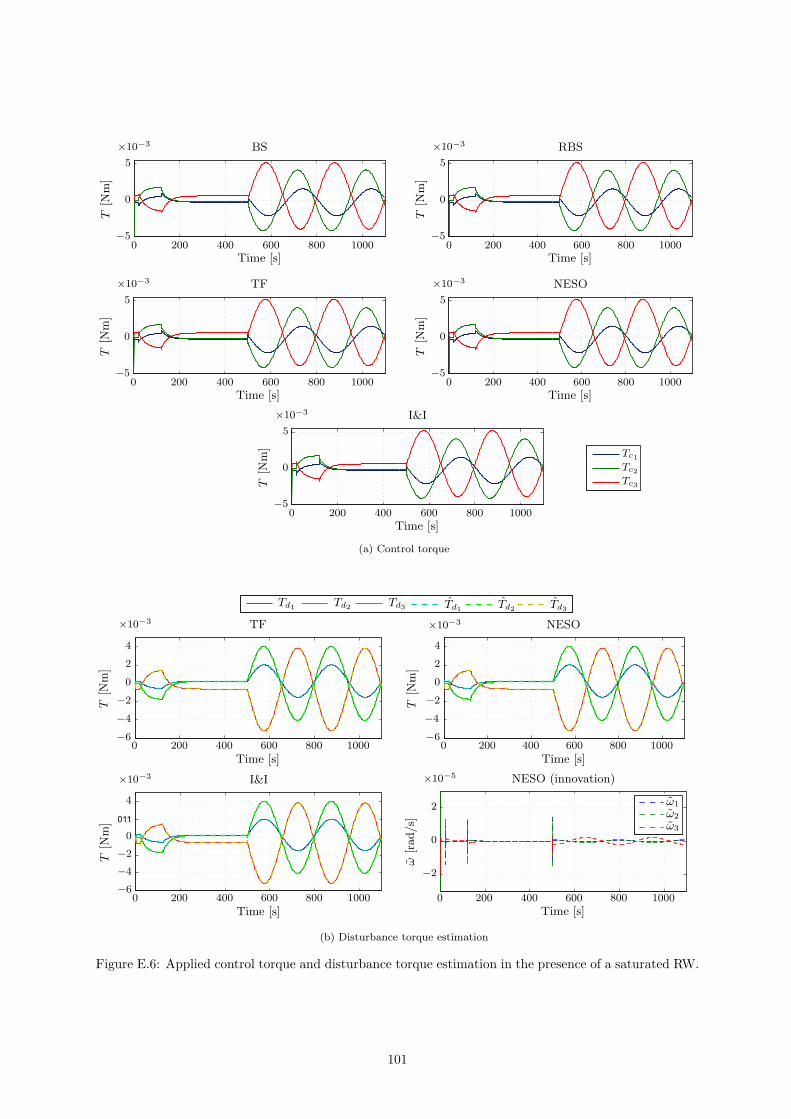
Tc3
Tc2
Tc1
T[N
m]
Time [s]
T[N
m]
Time [s]
T[N
m]
Time [s]
T[N
m]
Time [s]
T[N
m]
Time [s]
I&I
NESOTF
RBSBS
0 200 400 600 800 1000
0 200 400 600 800 10000 200 400 600 800 1000
0 200 400 600 800 10000 200 400 600 800 1000
×10−3
×10−3×10−3
×10−3×10−3
−5
0
5
−5
0
5
−5
0
5
−5
0
5
−5
0
5
(a) Control torque
011
Td3Td2Td1
ω3
ω2
ω1
Td3Td2Td1
T[N
m]
Time [s]Time [s]
T[N
m]
Time [s]
T[N
m]
Time [s]
ω[rad/s]
I&I
NESOTF
NESO (innovation)
00 200200 400400 600600 800800 10001000
0 200 400 600 800 10000 200 400 600 800 1000
×10−3×10−3
×10−3 ×10⁻⁵
−6
−4
−2
0
4
−6
−4
−2
0
2
4
−6
−4
−2
0
2
4
−2
0
2
(b) Disturbance torque estimation
Figure E.6: Applied control torque and disturbance torque estimation in the presence of a saturated RW.
101
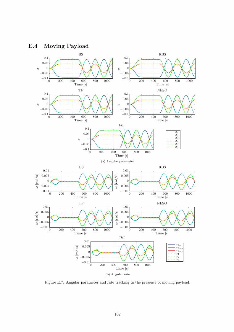
E.4 Moving Payload
σ3
σ2
σ1
σ3r
σ2r
σ1r
σ
Time [s]
σTime [s]
σ
Time [s]σ
Time [s]
σ
Time [s]
I&I
NESOTF
RBSBS
0 200 400 600 800 1000
0 200 400 600 800 10000 200 400 600 800 1000
0 200 400 600 800 10000 200 400 600 800 1000
−0.1
−0.05
0
0.05
0.1
−0.1
−0.05
0
0.05
0.1
−0.1
−0.05
0
0.05
0.1
−0.1
−0.05
0
0.05
0.1
−0.1
−0.05
0
0.05
0.1
(a) Angular parameter
ω3
ω2
ω1
x2,c3
x2,c2
x2,c1
ω[rad/s]
Time [s]
ω[rad/s]
Time [s]
ω[rad/s]
Time [s]
ω[rad/s]
Time [s]
ω[rad/s]
Time [s]
I&I
NESOTF
RBSBS
0 200 400 600 800 1000
0 200 400 600 800 10000 200 400 600 800 1000
0 200 400 600 800 10000 200 400 600 800 1000
−0.01
−0.005
0
0.005
0.01
−0.01
−0.005
0
0.005
0.01
−0.01
−0.005
0
0.005
0.01
−0.01
−0.005
0
0.005
0.01
−0.01
−0.005
0
0.005
0.01
(b) Angular rate
Figure E.7: Angular parameter and rate tracking in the presence of moving payload.
102

Tc3
Tc2
Tc1
T[N
m]
Time [s]
T[N
m]
Time [s]
T[N
m]
Time [s]T
[Nm]
Time [s]
T[N
m]
Time [s]
I&I
NESOTF
RBSBS
0 200 400 600 800 1000
0 200 400 600 800 10000 200 400 600 800 1000
0 200 400 600 800 10000 200 400 600 800 1000
×10−3
×10−3×10−3
×10−3×10−3
−1
−0.5
0
0.5
1
−1
−0.5
0
0.5
1
−1
−0.5
0
0.5
1
−1
−0.5
0
0.5
1
−1
−0.5
0
0.5
1
Figure E.8: Applied control torque in the presence of moving payload.
ω3
ω2
ω1
ω[rad/s]
Time [s]
NESO (innovation)
0 100 200 300 400 500 600 700 800 900 1000 1100
×10−5
−2
−1
0
1
2
Figure E.9: NESO rate estimation error (innovation) in the presence of moving payload.
103
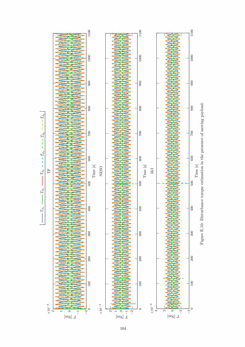
Td3
Td2
Td1
Td3
Td2
Td1
T[Nm]
Tim
e[s]
T[Nm]
Tim
e[s]
T[Nm]
Tim
e[s]
I&I
NESO
TF
0100
200
300
400
500
600
700
800
900
1000
1100
0100
200
300
400
500
600
700
800
900
1000
1100
0100
200
300
400
500
600
700
800
900
1000
1100
×10−4
×10−4
×10−4
−4
−2024
−2
−1012
−2
−1012
Figure
E.10:
Disturban
cetorqueestimationin
thepresence
ofmovingpayload
.
104