UNIVERSIDADE DA BEIRA INTERIOR Engenharia

Space Tether Systems Uniform Rotations of a Dumbbell-like System

Simão António da Rocha e Brito de Aguiã Morant

Dissertação para obtenção do Grau de Mestre em

Engenharia Aeronáutica (Ciclo de Estudos Integrado)

´

Orientador: Prof. Doutora Anna D. Guerman Co-orientador: Prof. Doutor Denilson P. S. dos Santos

Co-orientador: Prof. Doutor Pedro V. Gamboa

Covilhã, Junho 2014

ii

Left blank

iii

Dedication

I would like to dedicate this work to a few special people to whom I’m really thankful:

To my girlfriend Joana, who had to endure my bad temper in my sleepless nights and never-

ending days.

To my parents, who believed me and made me believe.

To Prof. Denilson Santos and his wife Heliene, who have accompanied me tirelessly in my work,

and to whom I’m grateful for all the attention they had with me. I will never forget the siri

dance that inspired me with laughs through the last months.

And at last, but not least, Prof. Anna Guerman, who kindly guided me and offered me the

possibility to work in a field where dreams are beyond the sky.

iv

Left blank

v

Acknowledgment

I am grateful to Fundação para a Ciência e a Tecnologia, who offered me a research grant in

the context of this dissertation, and to Prof. Anna Guerman, who made this grant possible.

vi

Left blank

vii

Abstract

In this dissertation, a dumbbell-like system is analyzed, considering two mass points connected

by a massless and rigid tether with variable length; its center of mass moves along an elliptic

Keplerian orbit. This kind of a system, in a certain type of configurations, is a simple

conceptualization of a space elevator. The system motion is obtained using the Lagrangian

formulation in a central gravitational field. The laws of control are considered for the system’s

rotation around its center of mass; those include the uniform rotations or permanent

orientation with respect to the local vertical. The stability conditions are obtained for the first

case, analyzing the equation in variations and using the Floquet theory. The results show that

there are regions of eccentricities where stability is found. Lastly, a dynamic numerical

simulator is created, where the implementation of the results can be tested.

Key-words

Tether Systems, Space Elevator, Dumbbell-like System, Stability of Solutions, Floquet Theory,

Monodromy Matrix.

viii

Left blank

ix

Resumo

Nesta dissertação, um sistema tipo halteres é analisado, considerando dois pontos de massa

conectados com um cabo rígido, sem massa e com variações do comprimento, e com o centro

de massa movendo-se segundo uma órbita Kepleriana. Este tipo de sistema, num certo tipo de

configuração, é uma simples conceptualização do elevador espacial. O movimento do sistema

é obtido com recurso à Formulação Lagrangiana num Campo Gravitacional Central. As leis de

controlo são consideradas para uma rotação do sistema à volta do seu centro de massa. Essas

incluem rotações uniformes e uma orientação permanente. As condições de estabilidade para

o primeiro caso foram obtidas, analisando a respectiva equação em variações e utilizando a

Teoria de Floquet. Os resultados mostraram que existem intervalos dos valores de

excentricidade onde a estabilidade é encontrada. Por último, um simulador numérico e

dinâmico foi criado, para se testar a implementação destes resultados.

Palavras-chave

Sistemas Ligados por Cabos, Elevador Espacial, Sistema Tipo Halteres, Estabilidade, Teoria de

Floquet, Matriz de Monodromia.

x

Left blank

xi

Index

Chapter 1- Introduction ...................................................................................................................................................................................... 1

1.1 General Purpose ................................................................................................................................................................................. 2 Chapter 2- Literature Review .......................................................................................................................................................................... 3

2.1 Historical Perspective...................................................................................................................................................................... 3 2.2 The general concept ......................................................................................................................................................................... 3 2.3 Applications and missions of tethers in space structures.............................................................................................. 4 2.4 Attitude Control .................................................................................................................................................................................. 7

Gravity-gradient stabilization ........................................................................................................................................ 8 2.5 State of the art ..................................................................................................................................................................................... 9

Chapter 3– Mathematical model of a two body tethered satellite system (TSS)................................................................. 13 3.1 Introduction ...................................................................................................................................................................................... 13 3.2 Mathematical model ...................................................................................................................................................................... 14

3.2.1 Center of mass..................................................................................................................................................................... 15 3.2.2 Positions of the system ................................................................................................................................................... 15 3.2.3 Potential energy of the system ................................................................................................................................... 16 3.2.4 Kinetic energy of the system ........................................................................................................................................ 17 3.2.5 The Lagrangian equations of motion ....................................................................................................................... 18

Chapter 4– Control laws .................................................................................................................................................................................. 21 4.1 Uniform rotations ........................................................................................................................................................................... 21

Tether behavior .................................................................................................................................................................. 22 4.2 Permanent orientation ................................................................................................................................................................. 32

Tether behavior .................................................................................................................................................................. 33 Chapter 5– Stability conditions .................................................................................................................................................................... 39

5.1 Monodromy Matrix ........................................................................................................................................................................ 39 Chapter 6- Simulations..................................................................................................................................................................................... 45

6.1 Dynamic Behavior .......................................................................................................................................................................... 45 System Earth – Satellite – Ballast............................................................................................................................... 45 System Earth – Moon - Ballast .................................................................................................................................... 47 System Earth – ISS - Space Module ........................................................................................................................... 49 System Moon – SMART1 – Satellite .......................................................................................................................... 50 System Titan – SST1 – SSTM ........................................................................................................................................ 52

6.2 Tether actuating force .................................................................................................................................................................. 53 6.3 Energy analysis ................................................................................................................................................................................ 55

Chapter 7– Conclusions ................................................................................................................................................................................... 57 Bibliography .......................................................................................................................................................................................................... 59 Annex 1 .................................................................................................................................................................................................................... 61 Annex 2 .................................................................................................................................................................................................................... 63

xii

Left blank

xiii

List of Figures

Figure 1.1 Artist Concept of a Space Elevator, from NASA Online Image Gallery _____________________________________ 1 Figure 2.1 Konstantin Tsiolkovsky ______________________________________________________________________________________ 3 Figure 2.2.1 Deployment overview scheme from Bartoszek Engineering _____________________________________________ 4 Figure 2.3.1.a Communication Antenna ________________________________________________________________________________ 6 Figure 2.3.1.b Electrodynamic Power Generation ______________________________________________________________________ 6 Figure 2.3.1.c Mars Observer ____________________________________________________________________________________________ 6 Figure 2.3.1.d Comet Sample Return____________________________________________________________________________________ 6 Figure 2.3.2 Shuttle TSS-1 Mission concept ____________________________________________________________________________ 7 Figure 2.4.1 Acting forces on a dumbbell tether system _______________________________________________________________ 8 Figure 2.5.1 Crawler system____________________________________________________________________________________________ 10 Figure 2.5.2 Equilibrium configurations ______________________________________________________________________________ 12 Figure 3.1.1 Satellite system connected with a tether _________________________________________________________________ 13 Figure 3.1.2 Dumbbell-like system composed by a massless tether and two mass points. ___________________________ 14 Figure 4.1.1.1 Tether logarithmic ratio for different eccentricities and 𝜔 = 0 ______________________________________ 22 Figure 4.1.1.2 Tether logarithmic ratio for different eccentricities and 𝜔 = 1 ______________________________________ 22 Figure 4.1.1.3 Tether logarithmic ratio for different eccentricities and 𝜔 = 2 ______________________________________ 23 Figure 4.1.1.4 Tether logarithmic ratio for different eccentricities and 𝜔 = 3 ______________________________________ 23 Figure 4.1.1.5 Tether logarithmic ratio for different eccentricities and 𝜔 = 3/4 ___________________________________ 24 Figure 4.1.1.6 Tether logarithmic ratio for different eccentricities and 𝜔 = 5/4 ___________________________________ 24 Figure 4.1.1.7 Tether logarithmic ratio approximation comparison and 𝜔 = 0 ____________________________________ 25 Figure 4.1.1.8 Tether logarithmic ratio approximation comparison and 𝜔 = 1 ____________________________________ 26 Figure 4.1.1.9 Tether logarithmic ratio approximation comparison and 𝜔 = 4 ____________________________________ 26 Figure 4.1.1.10 Tether logarithmic ratio approximation comparison and 𝜔 = 3/4 ________________________________ 27 Figure 4.1.1.11 Approximation error for 𝑒 = 0.04 ____________________________________________________________________ 27 Figure 4.1.1.12 Approximation error for 𝑒 = 0.5 _____________________________________________________________________ 28 Figure 4.1.1.13 Tether logarithmic ratio - Contour Plot for 𝑒 = 0.1_________________________________________________ 29 Figure 4.1.1.14 Tether logarithmic ratio - Contour Plot for 𝑒 = 0.3_________________________________________________ 29 Figure 4.1.1.15 Tether logarithmic ratio - Contour Plot for 𝑒 = 0.5_________________________________________________ 30 Figure 4.1.1.16 Tether logarithmic ratio - Contour Plot for 𝑒 = 0.1 and periodic findings ________________________ 31 Figure 4.1.1.17 Tether logarithmic ratio - Contour Plot for 𝑒 = 0.3 and periodic findings ________________________ 31 Figure 4.1.1.18 Tether logarithmic ratio - Contour Plot for 𝑒 = 0.5 and periodic findings ________________________ 32 Figure 4.2.1.1 Tether logarithmic ratio for different eccentricities for 𝜑0 = 0 _____________________________________ 33 Figure 4.2.1.2 Tether logarithmic ratio for different eccentricities for 𝜑0 = 1 _____________________________________ 33 Figure 4.2.1.3 Tether logarithmic ratio for different eccentricities for 𝜑0 = 2 _____________________________________ 34 Figure 4.2.1.4 Tether logarithmic ratio for different eccentricities for 𝜑0 = 3 _____________________________________ 34 Figure 4.2.1.5 Tether logarithmic ratio approximation comparison with 𝜑0 = 0 __________________________________ 35 Figure 4.2.1.6 Tether logarithmic ratio approximation comparison with 𝜑0 = 1__________________________________ 35 Figure 4.2.1.7 Tether logarithmic ratio approximation comparison with 𝜑0 = 3/4 _______________________________ 36 Figure 4.2.1.8 Approximation error for eccentricity = 0.04 ___________________________________________________________ 36 Figure 4.2.1.9 Tether logarithmic ratio - Contour Plot for 𝑒 = 0.1 __________________________________________________ 37 Figure 4.2.1.10 Tether logarithmic ratio - Contour Plot for 𝑒 = 0.3_________________________________________________ 37 Figure 4.2.1.11 Tether logarithmic ratio - Contour Plot for 𝑒 = 0.5_________________________________________________ 38 Figure 5.1.1 Stability Indicator for 𝜔 = −4;−3;−2 ________________________________________________________________ 41 Figure 5.1.2 Stability Indicator for 𝜔 = 32; 52; 72 ___________________________________________________________________ 41 Figure 5.1.3 Stability Indicator for 𝜔 = 1 ____________________________________________________________________________ 42 Figure 5.1.4 Stability Indicator for 𝜔 = 0 ____________________________________________________________________________ 42 Figure 5.1.5 Contour Plot of the different values of stability _________________________________________________________ 44 Figure 6.1.1.1 Geostationary Satellite Simulation with 𝑚2 = 200 𝑘𝑔, 𝑙0 = 190 𝑘𝑚, 𝜑 = 0.08𝜈 +2.17398,𝑂𝑟𝑏𝑖𝑡 𝑛𝑢𝑚𝑏𝑒𝑟 = 2 ___________________________________________________________________________________________ 46 Figure 6.1.1.2 Geostationary Satellite Simulation zoom with 𝑚2 = 200 𝑘𝑔, 𝑙0 = 190 𝑘𝑚, 𝜑 = 0.08𝜈 +2.17398,𝑂𝑟𝑏𝑖𝑡 𝑛𝑢𝑚𝑏𝑒𝑟 = 4 ___________________________________________________________________________________________ 46 Figure 6.1.1.3 Observation Satellite Simulation with 𝑚2 = 200 𝑘𝑔, 𝑙0 = 134.56 𝑘𝑚, 𝜑 = −1.2𝜈 −0.816814,𝑂𝑟𝑏𝑖𝑡 𝑛𝑢𝑚𝑏𝑒𝑟 = 2 __________________________________________________________________________________________ 47 Figure 6.1.2 Earth – Moon - Ballast Simulation (Space Elevator) with 𝑚2 = 10 000 𝑘𝑔, 𝑙0 = 20% semi − latus −rectum, 𝜑 = 0,𝑂𝑟𝑏𝑖𝑡 𝑛𝑢𝑚𝑏𝑒𝑟 = 15 ___________________________________________________________________________________ 48 Figure 6.1.3.1 ISS Simulation Zoom with 𝑚2 = 3000 𝑘𝑔, 𝑙0 = 130 𝑘𝑚,𝜑 = 0.2 𝜈 + 1.05558,𝑂𝑟𝑏𝑖𝑡 𝑛𝑢𝑚𝑏𝑒𝑟 = 2 ___________________________________________________________________________________________________________________________ 49 Figure 6.1.3.2 ISS Simulation with 𝑚2 = 15000 𝑘𝑔, 𝑙0 = 135.94 𝑘𝑚, 𝜑 = 0,𝑂𝑟𝑏𝑖𝑡 𝑛𝑢𝑚𝑏𝑒𝑟 = 20 ________________ 50 Figure 6.1.4 SMART1 Simulation with 𝑚2 = 2130 𝑘𝑔, 𝑙0 = 129.56 𝑘𝑚, 𝜑 = 0.2𝜈 + 2.11115,𝑂𝑟𝑏𝑖𝑡 𝑛𝑢𝑚𝑏𝑒𝑟 = 2 ___________________________________________________________________________________________________________________________ 51

xiv

Figure 6.1.5.1 SST1 Simulation with 𝑚2 = 100 𝑘𝑔, 𝑙0 = 147.56 𝑘𝑚, 𝜑 = −2.02664𝜈 −1.82007,𝑂𝑟𝑏𝑖𝑡 𝑛𝑢𝑚𝑏𝑒𝑟 = 2 __________________________________________________________________________________________ 52 Figure 6.1.5.2 SST1 Simulation with 𝑚2 = 100 𝑘𝑔, 𝑙0 = 147.56 𝑘𝑚, 𝜑 = 2.62574 − 1.82007,𝑂𝑟𝑏𝑖𝑡 𝑛𝑢𝑚𝑏𝑒𝑟 = 2 __________________________________________________________________________________________________________________________ 53 Figure 6.2.1 Earth – Satellite – Ballast variation force in function of 𝜈 for 𝑚2 = 200 𝑘𝑔, 𝑙0 = 130 𝑘𝑚, 𝜑 = 0.2ν +0.2, 𝑂𝑟𝑏𝑖𝑡 𝑛𝑢𝑚𝑏𝑒𝑟 = 4 ________________________________________________________________________________________________ 54 Figure 6.2.2 Earth – ISS – Space Module with 𝑚2 = 10 000 𝑘𝑔, 𝑙0 = 130 𝑘𝑚, 𝜑 = 0.2ν + 0.2, 𝑂𝑟𝑏𝑖𝑡 𝑛𝑢𝑚𝑏𝑒𝑟 = 4 __________________________________________________________________________________________________________________________ 54 Figure 6.2.3 Earth – ISS – Space Module with 𝑚2 = 10 000 𝑘𝑔, 𝑙0 = 130 𝑘𝑚, 𝜑 = 0.94ν +0.0628319,𝑂𝑟𝑏𝑖𝑡 𝑛𝑢𝑚𝑏𝑒𝑟 = 4________________________________________________________________________________________ 55 Figure 6.3.1 Kinetic energy for System Earth – ISS – Space Module with 𝑚2 = 10 000 𝑘𝑔, 𝑙0 = 130 𝑘𝑚, 𝜑 =0.2ν + 0.2, 𝑂𝑟𝑏𝑖𝑡 𝑛𝑢𝑚𝑏𝑒𝑟 = 8 ________________________________________________________________________________________ 56 Figure 6.3.2 Potential energy for System Earth – ISS – Space Module with 𝑚2 = 10 000 𝑘𝑔, 𝑙0 = 130 𝑘𝑚, 𝜑 =0.2ν + 0.2, 𝑂𝑟𝑏𝑖𝑡 𝑛𝑢𝑚𝑏𝑒𝑟 = 8 ________________________________________________________________________________________ 56 Figure A.2.1 Tether logarithmic ratio for different eccentricities and 𝜔 = 1/4 ____________________________________ 63 Figure A.2.2 Tether logarithmic ratio for different eccentricities and 𝜔 = 1/2 ____________________________________ 63 Figure A.2.3 Tether logarithmic ratio for different eccentricities and 𝜔 = −3 ______________________________________ 64 Figure A.2.4 Tether logarithmic ratio for different eccentricities and 𝜔 = −2 _____________________________________ 64 Figure A.2.5 Tether logarithmic ratio for different eccentricities and 𝜔 = −1/4 __________________________________ 65 Figure A.2.6 Tether logarithmic ratio for different eccentricities and 𝜔 = −1/2 __________________________________ 65 Figure A.2. 7 Tether logarithmic ratio for different eccentricities and 𝜔 = −3/4 __________________________________ 66 Figure A.2. 8 Tether logarithmic ratio for different eccentricities and 𝜔 = −5/4 __________________________________ 66 Figure A.2. 9 Tether logarithmic ratio for different eccentricities and 𝜔 = 3/4 ____________________________________ 67 Figure A.2. 10 Tether logarithmic ratio for different eccentricities and 𝜔 = 5/4 ___________________________________ 67 Figure A.2. 11 Tether logarithmic ratio for different eccentricities and 𝜔 = −3 ____________________________________ 68 Figure A.2. 12 Tether logarithmic ratio for different eccentricities and 𝜔 = −2 ____________________________________ 68 Figure A.2. 13 Tether logarithmic ratio for different eccentricities and 𝜔 = −3/4 _________________________________ 69 Figure A.2. 14 Tether logarithmic ratio for different eccentricities and 𝜔 = −5/4 _________________________________ 69

xv

List of Tables

Table 1. Stability conditions ................................................................................................................................................................... 43 Table 2. System Earth – Satellite – Ballast Properties ............................................................................................................... 45 Table 3. System Earth – Moon – Ballast Properties ..................................................................................................................... 48 Table 4. System Earth – ISS – Space Module Properties ............................................................................................................ 49 Table 5. Moon – SMART1 – Satellite Properties ............................................................................................................................ 51 Table 6. System Titan – SST1 – SSTM Properties .......................................................................................................................... 52 Table 7. TSS missions till 2013 .............................................................................................................................................................. 61

xvi

Left blank

xvii

List of Acronyms

UBI Universidade da Beira Interior

TSS Tethered Satellite System

CG Center of Gravity

CM Center of Mass

ISS International Space Station

𝑒 Eccentricity

𝜈 True anomaly

𝜑 Angle of rotation of the system around the center of mass

V Potential Energy

T Kinetic Energy

l Tether length

𝑙0 Initial tether length

𝑙𝑖 Length from the center of mass to point i

𝑚𝑖 Mass of point i

xviii

Left blank

1

Chapter 1 - Introduction

Nowadays, we foresee the future of our civilization as a high-tech society, where the space

journey makes part of our quotidian life. A society like that needs some robust infrastructures

that make possible the transport of merchandise and people. Space elevator is one of the best

options available, since it does not need rockets to reach space. Compared with rocket

propulsion [1], as V. Kaithi wrote, "the space elevator can provide easier, safer, faster and

cheaper access to space exploration".

An Earth space elevator is a transport system composed by a long tether, connecting Earth and

a ballast in a geostationary orbit. The cable will have to be very strong, since it will have some

physical challenges, as referred in Section 2.2. Despite those difficulties, the advances in

materials like carbon fibers do make this elevator possible, at least to be considered. Even

though we will not surely see this structure in the next years, there are being made interesting

analysis, studying the different aspects of such giant structure and developing technologies to

accomplish the main objective.

Artificial satellites have been suggested to launch the tether. The cable will start downwards,

from a geostationary orbit, and falling into Earth – in some point in the Equatorial line. To

conceptualize some missions, it is important to study the dynamics of such systems, and ensure

stability is achieved.

Figure 1.1 Artist Concept of a Space Elevator, from NASA Online Image Gallery

2

1.1 General Purpose

Since 1960th several researchers have been studying the possibilities to control attitude motion

of space systems with variable mass distributions with the intention to control spacecraft

dynamics. One of the purposes of this control can be implementation of a specific attitude

motion required by the mission and stabilization of such motion with respect to perturbations.

Here we consider dynamics of a two-body tether systems in a central Newtonian gravitational

field. The perturbations of motion can occur for several factors, such as atmospheric drag, solar

pressure, tether deployment, n-body perturbations, among others which are not discussed

here. We assume that the center of mass of the system moves along a Keplerian orbit and study

attitude dynamics, control, and stability of such dumbbell-like configuration. The motion’s

equation is written using Lagrangian formulation writing down the Kinetic and Potential Energy,

and considering the possibility to control the tether length to implement a specific rotation

around the system’s center of mass. We also present a numerical simulator created for this

goal.

3

Chapter 2 - Literature Review

2.1 Historical Perspective

In 1895, the Eiffel tower became the inspiration for Konstantin Tsiolkovsky. The Russian

scientist dedicated his life to the study of astronautics and rocket physics and, encouraged by

the tower, saw the opportunity to explore the outer space with the edification of a structure

that could reach the space. That structure, in Tsiolkovsky idea, would have a tether in the top

of it and it would extend for kilometers [2].

Although it seems a science fiction, just like in more than 80 sci-fi books and movies where

such space tower appears, , since the 1980s scientists have performed several studies to

evaluate a real scenario for space elevator (see, e.g., Swan and Swan [3]).

Figure 2.1 Konstantin Tsiolkovsky

2.2 The general concept

The first concept of a Space Elevator, as referred previously, is based on Tsiolkovksy's idea. He

regarded some problems mostly concerned with the structure itself. According to [4] some of

these problems were:

The tether material;

The susceptibility to vibrations;

4

The wobble from Coriolis force;

The space debris;

Social and Environmental Risks;

Collisions with meteoroids and micrometeorites;

Corrosion;

Radiation and consequent ionization.

The concept proposed by Edwards and Westling [5] consists in one long tether of about 1 meter

in width and of an insignificant thickness (macromolecules size), attached to Earth and

extending to the outer space. Figure 2.2.1 shows the concept and the deployment phases of

the space elevator.

Figure 2.2.1 Deployment overview scheme from Bartoszek Engineering

2.3 Applications and missions of tethers in space

structures

To understand the concept of a space elevator, it is important to comprehend the dynamics of

space systems connected with tethers. Space tether systems have been quite important in

space exploration, since first applied in Gemini XI, in 1966. After that, the tethers have been

used in several missions, providing passive attitude stabilization, while creating an artificial

gravity and reducing the need to use the propellant.

5

As a matter of fact, there have been lots of applications attributed to the space tethers. The

fundamental book of Beletsky and Levin [6] provides a review of a good amount of applications

and makes an interesting analysis of the dynamics of space tether systems.

In [7], Cartmell and McKenzie focus on some interesting applications:

Two-dimensional tethered constellations;

Construction of a passive space facility with tethers separating platforms;

Payload orbit raising and lowering;

Elevator using tethers to the orbit transfers (from LEO to GEO);

Tensions systems for solar sails.

Cosmo and Lorenzini [8] offer a good description of various applications. The list is very long

including:

Multiprobe for Atmospheric Studies

Gravity Wave Detection Using Tethers

Earth-Moon /Mars-Moon Tether Transport System

Rotating Controlled-Gravity Laboratory

Tethered Space Elevator

Electrodynamic Power and Thrust Generation

Communication Antenna

Aerocapture with Tethers for Planetary Exploration

Comet/Asteroid Sample Return

Mars Tethered Observer

Tethered Lunar Satellite for Remote Sensing

(see Figures 2.3.1)

6

Figure 2.3.1.a Communication Antenna Figure 2.3.1.b Electrodynamic Power

Generation

Figure 2.3.1.c Mars Observer Figure 2.3.1.d Comet Sample Return

As listed above, tethers do have an important role in future space exploration. In formation

flying systems, tethers are able to provide simple solutions to some problems of creating a

convenient nominal motion, e.g., a state of equilibrium. As referred in [9] by M. v. Pelt, the

different altitudes and the different time-launches of the satellites in formation or even the

fact that the Earth is not perfectly round, make them to orbit in slightly different velocities,

meaning they would drift away from each other, destroying therefore an intended formation

configuration. Although the propulsion systems are still capable to correct the trajectory, they

are limited and sometimes don’t provide the required precision. Tethers offer a direct physical

effect in the attitude control system, providing the means to the stabilization of the system.

We focus in this subject in Section 2.4.

7

Some missions using TSS have been quite significant. As referred before, Gemini XI was the first

one, using a tether to provide artificial gravity. John Hoffman et al. [10] analyze the dynamics

of the tether to provide artificial gravity for the ASTOR (Advanced Safety Tether Operation and

Reliability) project. In 1992, the mission Shuttle TSS-1 tested the TSS concept on the Space

Shuttle, where the dynamics of TSS were evaluated [11] (see Figure 2.3.2). PMG mission

successfully tested an electrodynamic tether [12], being able to convert electricity from orbital

energy. In Table 2 [13] (see Annex 1) one can see numerous TSS missions. The same article

explores all the mission’s details. One important application conferred to space tether systems

could be the use of net systems connected with tethers for debris capture and removal [14], as

in 2010 the percentage of drift objects (space debris) in orbit around Earth were about 49% of

the total.

Figure 2.3.2 Shuttle TSS-1 Mission concept

2.4 Attitude Control

Attitude control, according to [15], refers to “maintenance of a desired, specified attitude

within a given tolerance”. Correctly determined, it allows the satellite system to be correctly

oriented in the required orbit, giving some adjusts in its orientation over time and correcting

perturbations. Those adjustments can be done in different ways:

Spin stabilization;

Momentum wheels;

Control moment gyros;

Solar sails;

8

Gravity-gradient stabilizations;

Etc.

The corrections in attitude usually need sensors for measuring the position in the orbit frame.

Gravity-gradient stabilization

Satellite tether systems can use the tether to provide gravity-gradient stabilization. This

passive stabilization, also known as tidal stabilization, uses the appropriate body mass

distribution and the gravitation field applied and does not require an active control system with

sensors and actuators.

Consider a motion in a circular orbit of a simple dumbbell-like system, composed by two masses

connected with a tether. When aligned with the local vertical, the two masses experiment

different forces, as shown in Figure 2.4.1. The centrifugal force is larger in the upper element,

but the gravitational force is weaker. On the contrary, the gravity force acting on the lower

mass is larger, but the respective centrifugal force is weaker.

Figure 2.4.1 Acting forces on a dumbbell tether system

As one can notice (see, e.g., [8]), the resultant forces act on the system as a stabilization

mechanism, forcing it into a vertical orientation. Therefore the system possesses two stable

9

equilibrium configurations, one shown in Figure 2.4.1, and the other inverse with respect to

the local horizontal. (Note that for the case of a three-dimensional asymmetric rigid body, the

same physical mechanism results in 24 equilibrium configurations, four of which are stable1.)

The above example shows that for the motion in orbital environment the center of mass (cm)

of the system normally doesn’t coincide with its center of gravity (cg). Moreover, it is clear

that the orbital motion of a large space system, such as a large tethered structure, cannot be

separated from its attitude motion and therefore its orbit differs from the orbit of a point with

the same mass (that is, from the respective Keplerian orbit). However, when the tether lengths

are not too large, this difference is extremely small and will be neglected here.

2.5 State of the art

Some of the recent efforts done on the study of dynamic and control of space tethers systems

show that the gravity-gradient is a natural and elegant solution to provide stabilization [10]

[16]. However, some problems have been identified and referred to in several articles [17] [18]

[19].

In [17], E.C. Lorenzini and J. Ashenberg note that the tether can be sometimes misaligned with

respect to the local vertical at the center of mass. The orbital eccentricity itself produces small

perturbations that influence the system stability. The same authors suggest an active

stabilization mechanism based on the torque provided by the tether’s tension. That mechanism

can be implemented linking the tether to a rigid attachment fixed in the space station and

adding a torque motor to it. This way, the torque is controlled actively. The authors developed

a LQR (Linear Quadratic Regulator) controller taking into account the eccentricity of the

Keplerian orbit, while the other papers at the time considered only circular orbits.

In [18] and [19], M. Pascal studies control laws for the tether deployment and retrieval. She

states that in almost all studies, the law of deployment/retrieval is chosen “a priori” as linear

or exponential law. The author combines different laws for fast and simple motions with

analytical solutions for in-plane and out-of-plane motions, for massless and massive tethers and

for circular and elliptical orbits. In the first article M. Pascal focuses on a crawler system, where

a sub-satellite climbs the tether towards the Space Station, contrary to the notion of the tether

being pulled to it. A scheme of a possible crawler system is represented in Figure 2.5.1 [20].

1 P. C. Hughes, Spacecraft Attitude Dynamics. Dover Publications, 2004, 592 pp.

10

Figure 2.5.1 Crawler system

A. Djebli and M. Pascal deepen the study of advantages for the crawler system in [21], resulting

in faster variation of the orbital parameters compared to conventional methods. The article

suggests this system to attain orbital modifications. As a negative consequence, the change in

absolute energy and the tether tension variations are higher than usual. A relevant adding are

the radial and azimuthal accelerations trough Earth, causing some perturbations in the motion.

Some TSS state of the art applications have already been mentioned in Section 2.3. The review

article of Cartmell & McKenzie [7] refers to the use of tethers as tension mechanisms in solar

sail structures for trajectory corrections. An electrodynamic tether system can also create an

artificial electric field, transferring momentum from charged particles of the solar wind to the

system. The respective propulsion system e-sail (from solar wind electric sail, [22]) is already

being tested in the ESTCube-1, ESA satellite. Tethers can also provide links for lower-altitude

payloads and high-altitude solar sails and cube sails. An example of a cube sail is considered in

[23], with a tether being a 260m long reflecting film. The ProSEDS mission, listed in Table 7

(Annex 1), was supposed to launch an electrodynamic tether system, with 15 km of length, in

which 10 km would be of insulated material, and the remaining would be conductor. The

mission was cancelled because of the possibility to collide with the ISS. Collisions problems

between tethers in de-orbiting missions are also referred by [7], noting that if 40 de-orbits via

TSS happens in a year, it means that only 4 tethers are in the space at a certain time, which

reduce the probability of collisions events. The review article [7] does an exhaustive study of

tethers.

11

Several authors study attitude dynamics of TSS in different configurations. Two-body and three-

body systems have been mostly studied, but even tethered satellite constellations have been

analyzed. In [24] the dynamics of three-body TSS is examined, with the cm following a circular

orbit. A similar geometrical draw of the system is retracted in Chapter 3. In the referred article,

a constant tether length constraint is also considered and equilibrium configurations are

presented, as seen in Figure 2.5.2. Numerical results are given for several tether parameters,

including tether lengths, tether speeds variations, and tether tensions. A dual spacecraft

configuration that uses tethers for body connection [25], is suggested, with some interesting

arrangements: parallel, parachute and single tether-connected body geometries.

In [26] and [27], A. Guerman considers the general problem of steady-state motions of a

tethered satellite system in a circular orbit. All in-plane equilibrium configurations for arbitrary

satellite masses and the tether lengths are found analytically in [26]. In [27] all possible spatial

equilibrium configurations are described, and several classes of three-dimensional tethered

formations are found. Tetrahedral formations which are of special interest for space

applications are examined in detail, including the stability analysis, by Guerman et al. in [28].

In [29], S. Yu presents a control law for the tether length (known as range rate control

algorithm) and demonstrates the equilibrium state as a function of the rotation angle. A circular

and an orbital case are analyzed. Perturbations of motion are considered, namely the

gravitational, centrifugal, and Coriolis forces.

A. K. Misra [30] addresses the nonlinear motions of a three dimensional TSS. Hamiltonian

formulation is used and Poincaré sections for planar (pitch) and coupled motion (pitch and roll)

are shown [31]. Non-chaotic motion is found for pitch and roll angles inferior or equal to 26˚,

as the Lyapunov exponent approaches zero over time. The same article evaluates the effect of

aerodynamic and electrodynamic forces as well as the lifetime prediction and orbital decay of

the system.

A. Burov, I. Kosenko, and A. Guerman in [32] study the dynamics of a moon-anchored tether

with a material point at its end for variable tether length. The two-dimensional problem is

addressed as a simple model for the lunar elevator. In this problem, some particular solutions

of the motion equation are derived, choosing a specific control law for the tether length and

finding radial and oblique configurations for the system geometry, while defining regions of

stability and instability for each case.

12

Figure 2.5.2 Equilibrium configurations

In [33] (W. Zhang and M. Yao), the periodic solution and stability of a tethered satellite system

are found. As the authors refer, and should be cited, “the total mechanical energy of the system

is minimum when the motion coincides with the periodic solution”, implying that “the periodic

solution is the minimum energy solution, and the periodic solution in an elliptic orbit has the

same significance as the equilibrium state in a circular orbit from the mechanical point of

view”. The search of periodic solutions provides information about the equilibrium and/or

critical solutions.

In [34], dynamics of a dumbbell composed by two masses connected by a lightweight tether is

analyzed in an elliptic orbit. The system can serve as a simplified model for a two-body tether

connected spacecraft. The article focuses on a specific tether control law to guarantee a

uniform rotation of the system in terms of the true anomaly. Study of chaotic and regular

motion, as well as stability analysis are also done.

13

Chapter 3 – Mathematical model of a

two body tethered satellite system

(TSS)

3.1 Introduction

The main objective of this dissertation is to analyze dynamics of a two bodies TSS in an elliptical

orbit. The image of such system can be seen in Figure 3.1.1. The model is a dumbbell-like

system, with the two mass points connected with a rigid and massless tether. The system’s

center of mass moves along an elliptic Keplerian orbit fixed in an inertial reference frame EXY

connected to the center of the Earth (Fig. 3.1.2).

Figure 3.1.1 Satellite system connected with a tether

For the following analysis, each satellite is considered as a mass point and the tether is assumed

to be massless. In this model, the positions of the two mass points are described with respect

to the position of the center of mass of the system (C). The angles υ and φ represent the true

anomaly and the angle between the tether and the position vector of the cm EC, respectively,

ρ is the distance from E to C, l1and l2 are the distances between the mass points m1 and m2

and C, respectively, the length of the tether is 𝑙 = 𝑙1 + 𝑙2.

14

Figure 3.1.2 Dumbbell-like system composed by a massless tether and two mass points.

3.2 Mathematical model

The mathematical model is obtained in the following steps [34]:

i. Position of the center of mass based on 𝑙1and 𝑙2 lengths;

ii. ρ, r1and 𝑟2 description based on Keplerian orbits;

iii. Potential Energy;

iv. Kinetic Energy;

v. Lagrange Equations of Motion.

15

3.2.1 Center of mass

Remembering the definition of the center of mass, and considering

𝑙 = 𝑙1 + 𝑙2 ( 1 )

(Figure 3.1.2), one obtains:

𝑚1 ∗ 𝑙1 = 𝑚2 ∗ 𝑙2

( 2 )

Substituting Equation ( 1 ) in to Equation ( 2 ), arrives at:

𝑙1 =𝑚2 ∗ 𝑙

𝑚1 + 𝑚2

( 3 )

𝑙2 =𝑚1 ∗ 𝑙

𝑚1 + 𝑚2

( 4 )

With these equations, the length of each part of the tether is known in function of the masses

𝑚1, 𝑚2, and the total tether length 𝑙.

3.2.2 Positions of the system

As stated before (see Section 2.4), we consider here that the size of the system is small

compared to the orbit dimensions, which allows the motion to be described by the Keplerian

formula:

𝜌 =𝑝

1 + 𝑒 ∗ 𝑐𝑜𝑠(𝜈)

( 5 )

with

𝑝 as the focal parameter,

e as the eccentricity,

𝜈 as the true anomaly

The meaning of the above parameters can be seen in [35] (Chapter 2). The system coordinates

are:

𝑥0 = 𝜌 ∗ 𝑐𝑜𝑠 (𝜈)

𝑦0 = 𝜌 ∗ 𝑠𝑖𝑛 (𝜈) ( 6 )

𝑥1 = 𝑥0 + 𝑙1 ∗ 𝑐𝑜𝑠 (𝜈 + 𝜑)

𝑦1 = 𝑦0 + 𝑙2 ∗ 𝑠𝑖𝑛 (𝜈 + 𝜑)

16

𝑥2 = 𝑥0 − 𝑙2 ∗ 𝑐𝑜𝑠 (𝜈 + 𝜑)

𝑦2 = 𝑦0 − 𝑙2 ∗ 𝑠𝑖𝑛 (𝜈 + 𝜑)

where

𝑥0 and 𝑦0 are the components of the position vector of the center of mass, 𝑟0⃗⃗ ⃗

𝑥1 and 𝑦1 are the components of the position vector of the point mass 1, 𝑟1⃗⃗⃗

𝑥2 and 𝑦2 are the components of the position vector of the point mass 2, 𝑟2⃗⃗ ⃗

{

𝑟0⃗⃗ ⃗ = (𝑥0, 𝑦0)

𝑟1⃗⃗⃗ = (𝑥1, 𝑦1)

𝑟2⃗⃗ ⃗ = (𝑥2, 𝑦2)

( 7 )

3.2.3 Potential energy of the system

The potential energy of the system can be obtained using the following expression:

𝑉 = −∑𝜇0 ∗ 𝑚𝑖

‖𝑟𝑖⃗⃗ ‖

𝑛

𝑖=1

( 8 )

where:

n represents the number of total mass points of the system

𝑚𝑖 represents the mass of the point

𝑟𝑖⃗⃗ represents the position vector of the point mass with respect to the Earth’s center

𝜇0 = 𝐺 ∗ 𝑀

G represents the universal gravitational constant

M is the mass of the Earth

For the problem in study, Equation ( 8 ) reads

𝑉 = −𝜇0 ∗ 𝑚1

‖𝑟1⃗⃗⃗ ‖−

𝜇0 ∗ 𝑚2

‖𝑟2⃗⃗ ⃗‖

( 9 )

Introducing two new variables 𝜇 and 𝑚:

17

𝜇 =𝑚1

𝑚

( 10 )

𝑚 = 𝑚1 + 𝑚2

( 11 )

Equation ( 9 ) becomes:

𝑉 = −𝜇0 ∗ 𝑚 (𝜇

‖𝑟1⃗⃗⃗ ‖+

1 − 𝜇

‖𝑟2⃗⃗ ⃗‖)

( 12 )

or

𝑉 = −𝜇0 ∗ 𝑚 (𝜇

√𝑥12 + 𝑦1

2+

1 − 𝜇

√𝑥22 + 𝑦2

2)

( 13 )

Introducing a new variable λ,:

𝜆 =𝑙

𝑝

( 14 )

and assuming λ ≪ 1, i.e., the tether length is much smaller than the focal parameter 𝑝, one

can write the Taylor series expansion of 2nd order for 𝑉 as:

𝑉 = −𝑚 𝜇0 (1 + 𝑒 ∗ 𝑐𝑜𝑠(𝜈))

𝑝+

𝑚 (−1 + 𝜇) 𝜇 𝜇0 (1 + 𝑒 ∗ 𝑐𝑜𝑠(𝜈))3 (1 + 3 ∗ 𝑐𝑜𝑠(2 𝜑))𝜆2

4𝑝

( 15 )

Here we omit the terms of the third and higher orders with respect to λ.

3.2.4 Kinetic energy of the system

The kinetic energy of the system can be obtained using the following equation:

𝑇 = ∑𝑚𝑖 ∗ 𝑣𝑖

2

2

𝑛

𝑖=1

( 16 )

where

n represents the number of total mass points of the system

𝑚𝑖 represents the mass of the point i

18

𝜈𝑖⃗⃗ represents the vector velocity of the point mass i

Since

𝑣𝑖 = ‖𝑟𝑖⃗⃗ ‖̇

( 17 )

while denoting

( )̇ =𝑑

𝑑𝑡

( 18 )

one obtains

𝑣𝑖 = √𝑥�̇�2 + 𝑦�̇�

2

( 19 )

Returning to Equation ( 16 ),

𝑇 =𝑚1 ∗ (𝑥�̇�

2 + 𝑦�̇�2)

2+

𝑚2 ∗ (𝑥2̇2 + 𝑦2̇

2)

2

( 20 )

𝑇 =1

4𝑚 [

2𝑝2(1 + 𝑒2 + 2𝑒 𝑐𝑜𝑠 𝜈)�̇�2

(1 + 𝑒 𝑐𝑜𝑠 𝜈)4− 2(−1 + 𝜇)𝜇(𝑙2̇ + 𝑙2(�̇� + �̇�)2)]

( 21 )

3.2.5 The Lagrangian equations of motion

The Lagrangian equations of motion are known as differential equations of system motion in

generalized coordinates. In fact, the Lagrangian equations provide a simple way to obtain the

system positions in function of time [36, 37]. It was decided to choose the Lagrangian

formulation because it allows us to define the global positions of the system through potential

and kinetic energy and in function of generalized coordinates, unlike the needs to define all

the forces and coordinates involved, as in Newtonian formulation.

The Lagrangian equation is:

𝑑

𝑑𝑡(

𝜕𝐿

𝜕�̇�𝑗

) −𝜕𝐿

𝜕𝑞𝑗

= 𝑄𝑗

( 22 )

where 𝐿 = 𝑇 − 𝑉 , 𝑞𝑗 is the generalized coordinate and 𝑄𝑗 is the generalized force actuating in

the system.

19

For the conservative case one has:

𝑑

𝑑𝑡(

𝜕𝐿

𝜕�̇�𝑗

) −𝜕𝐿

𝜕𝑞𝑗

= 0

( 23 )

For the following analysis, the generalized coordinates are 𝜑 and 𝑙 and the system is only under

the gravitational forces. Two equations can be obtained:

𝑑

𝑑𝑡(𝜕𝐿

𝜕�̇�) −

𝜕𝐿

𝜕𝜑= 0

𝑑

𝑑𝑡(𝜕𝐿

𝜕𝑙̇) −

𝜕𝐿

𝜕𝑙= 0

( 24 )

Defining 𝜑 or 𝑙 as a function of time allows one to find the remaining parameter as a control

for system, as can be seen in Chapter 4. It has been chosen to define the desirable law for re-

orientation 𝜑 = 𝜑(𝑡) and obtain the respective control law for the tether length 𝑙 = 𝑙(𝑡).

Therefore, the first equation in Equations ( 24 ) should be studied. After some simplifications,

it becomes:

𝑙 (3 𝜇0 𝑠𝑖𝑛(2𝜑)(𝑒 cos(𝜈) + 1)3 + 2𝑝3(�̈� + �̈�)) + 4𝑝3𝑙(̇�̇� + �̇�) = 0

( 25 )

All these variables are time-related. For a more advantageous formulation, consider new

independent variable, the true anomaly 𝜈. A new change of variables and definitions is

introduced:

( )′ =𝑑

𝑑𝜈

( 26 )

�̇� = 𝜔0(1 + 𝑒 𝑐𝑜𝑠 𝜈)2

( 27 )

with

𝜔02 =

𝜇0

𝑝3

( 28 )

The chain rule applies here, where

(𝑓 𝑜 𝑔)′(𝑐) = (𝑓′𝑜 𝑔)(𝑐) ∗ 𝑔′(𝑐) ( 29 )

and �̈� becomes

ν̈ = −2𝑒 𝜇0 𝑠𝑖𝑛 (𝜈)(𝑒 𝑐𝑜𝑠 𝜈 + 1)3

𝑝3

( 30 )

20

For the other parameters, the same change occurs, although the result is suppressed:

�̇� = 𝜑′ ∗ �̇�

( 31 )

�̈� = 𝜑′′ ∗ �̇� ∗ �̇� + 𝜑′ ∗ �̈�

( 32 )

𝑙 ̇ = 𝑙′ ∗ �̇�

( 33 )

𝑙 ̈ = 𝑙′′ ∗ �̇� ∗ �̇� + 𝑙′ ∗ �̈�

( 34 )

Substituting all these variables, Equation ( 25 ) becomes:

(𝑒 𝑐𝑜𝑠(𝜈) + 1) (4𝑙′ (𝜑′ + 1)(𝑒 𝑐𝑜𝑠(𝜈) + 1)

+ 𝑙(2𝜑′′(𝑒 𝑐𝑜 𝑠 𝜈 + 1) − 4𝑒 𝑠𝑖𝑛(𝜈)𝜑′ − 4𝑒 𝑠𝑖𝑛(𝜈) + 3 𝑠𝑖𝑛(2𝜑))) = 0

( 35 )

which can be rearranged as

(1 + 𝑒 𝑐𝑜𝑠 𝜈) ∗ 𝜑′′ + 2 [𝑙′

𝑙∗ (1 + 𝑒 𝑐𝑜𝑠 𝜈) − 𝑒 ∗ 𝑠𝑖𝑛 𝜈] (1 + 𝜑′) + 3 𝑐𝑜𝑠𝜑 𝑠𝑖𝑛𝜑 = 0

( 36 )

a well-known equation [34] [38]. Note that this equation does not depend on the mass of the

system.

21

Chapter 4 – Control laws

At this stage, the Lagrangian equations of motion have been derived. Now we can choose the

desired variation of the system’s attitude 𝜑 = 𝜑(𝜈) (the programmed re-orientation of the

tether) and obtain the equation for the respective control law for the tether length 𝑙 = 𝑙(𝜈).

Two modes of the behavior of 𝜑 are presented: the uniform rotations and fixed orientation with

respect to the local vertical. Each case is analyzed independently.

4.1 Uniform rotations

For uniform rotations, the control law can assume the following form [34] [39]:

𝜑 = 𝜔 𝜈 + 𝜑0

( 37 )

This relation means that the actual angle of rotation depends on the initial condition 𝜑0, the

variation of 𝜈 and a constant 𝜔 (angular velocity).

Equation ( 36 ) can be rewritten:

2 [𝑙′

𝑙(1 + 𝑒 𝑐os(𝜈)) − 𝑒 sin(ν)] (1 + ω) − 3 cos(ω 𝜈 + 𝜑0 ) sin(ω 𝜈 + 𝜑0) = 0

( 38 )

Resolving this equation for 𝑙´

𝑙, yields

𝑙′

𝑙=

2𝑒 sin ν + 2𝑒 𝜔 𝑠in 𝜈 − 3𝑐os(𝜔𝜈 + 𝜑0)sin(𝜔𝜈 + 𝜑0)

2(1 + 𝜔)(1 + 𝑒 𝑐os 𝜈)

( 39 )

which is equivalent to

𝑙′

𝑙=

𝑒 𝑠𝑖𝑛 𝜈

1 + 𝑒 𝑐𝑜𝑠 𝜈−

3 𝑠𝑖𝑛 (2(𝜔𝜈 + 𝜑0))

4(1 + 𝜔)(1 + 𝑒 𝑐𝑜𝑠 𝜈)

( 40 )

22

Tether behavior

Equation ( 40 ) allows one to obtain the tether length l as a function of 𝜈. However, in the

general case, analytical integration of (40) is not possible. For some values of 𝜔 the control law

can be obtained in the close form; for other values of angular velocity 𝜔 the integration has to

be performed numerically.

Here, some results are presented assuming that 𝜑0 = 0.

Figure 4.1.1.1 Tether logarithmic ratio for different eccentricities and 𝜔 = 0

Figure 4.1.1.2 Tether logarithmic ratio for different eccentricities and 𝜔 = 1

23

Figure 4.1.1.3 Tether logarithmic ratio for different eccentricities and 𝜔 = 2

Figure 4.1.1.4 Tether logarithmic ratio for different eccentricities and 𝜔 = 3

It is interesting to note that all the tether variations for those 𝜔 seem to be periodic. One can

see that with increase of 𝜔, the logarithmic curves have more oscillations, those being more

noticable for small values of eccentricity. Inverse rotations (𝜔 < 0) are similar to those

24

presented (see Annex 2). For fractional values of 𝜔, the tether may not assume a 2𝜋 periodic

behavior.

Figure 4.1.1.5 Tether logarithmic ratio for different eccentricities and 𝜔 = 3/4

Also, as can be seen from Equation (38), for 𝜔 = −1 the solutions do not exist.

Figure 4.1.1.6 Tether logarithmic ratio for different eccentricities and 𝜔 = 5/4

For more simulations, see Annex 2.

25

Although an analytical integration of Equation ( 40 ) is not possible, an approximation has been

made to obtain a general formulation of the tether length for each 𝜈. The results use the Taylor

series of the 4th order and are presented below.

The approximation of the right-hand term of Equation ( 40 ) is:

𝑒4 (−3 𝑐𝑜𝑠4(𝜈) 𝑠𝑖𝑛(2𝜈𝜔)

4(𝜔 + 1)− 𝑠𝑖𝑛(𝜈) 𝑐𝑜𝑠3(𝜈))

+ 𝑒3 (3 𝑐𝑜𝑠3(𝜈) 𝑠𝑖𝑛(2𝜈𝜔)

4(𝜔 + 1)+ 𝑠𝑖𝑛(𝜈) 𝑐𝑜𝑠2(𝜈))

+ 𝑒2 (−3 𝑐𝑜𝑠2(𝜈) 𝑠𝑖𝑛(2𝜈𝜔)

4(𝜔 + 1)− 𝑠𝑖𝑛(𝜈) 𝑐𝑜𝑠(𝜈))

+ 𝑒 (3 𝑐𝑜𝑠(𝜈) 𝑠𝑖𝑛(2𝜈𝜔)

4(𝜔 + 1)+ 𝑠𝑖𝑛(𝜈)) −

3 𝑠𝑖𝑛(2𝜈𝜔)

4(𝜔 + 1)

( 41 )

considering 𝑒 ≪ 1. This expression allows integration, though the results are quite cumbersome

and are omitted here. Some results are plotted below.

Figure 4.1.1.7 Tether logarithmic ratio approximation comparison and 𝜔 = 0

26

Figure 4.1.1.8 Tether logarithmic ratio approximation comparison and 𝜔 = 1

Figure 4.1.1.9 Tether logarithmic ratio approximation comparison and 𝜔 = 4

The simulations above are made for 𝑒 = {0.04 , 0.1 ,0.3, 0.5}. Note the similarity between the

direct integration and the use of the approximation. Even for the fractional values of the

angular velocity the approximation via Taylor series is very precise (see Figure 4.1.1.10).

27

Figure 4.1.1.10 Tether logarithmic ratio approximation comparison and 𝜔 = 3/4

The error of the approximation for 𝜔 = 0 and for 𝑒 = 0.04 and 𝑒 = 0.5, can be seen in Figures

4.1.1.11 and 4.1.1.12.

Figure 4.1.1.11 Approximation error for 𝑒 = 0.04

28

Figure 4.1.1.12 Approximation error for 𝑒 = 0.5

The error increases as eccentricity also increases, since the approximation has been made

considering 𝑒 ≪ 1. Simulations for other values of 𝜔 and 𝑒 result in similar error ranges.

It should be noted this approximation introduces some new critical cases, where solutions don’t

exist. These critical cases correspond to 𝜔 = {0;1

2; 1;

3

2; 2; −

1

2; −

3

2; −2}, as indeterminations

appear. Although some of the graphics using the approximation for those 𝜔 are presented in

this document, the neighborhood was taken into account.

The contour plots can also be a good tool to illustrate the tether behavior as function of 𝜔 and

𝑒. At Figures 4.1.1.13 - 4.1.1.15 it is possible to see the logarithmic values of the tether ratio

𝑙

𝑙0 for some eccentricities (the color legend refers to those values):

29

Figure 4.1.1.13 Tether logarithmic ratio - Contour Plot for 𝑒 = 0.1

Figure 4.1.1.14 Tether logarithmic ratio - Contour Plot for 𝑒 = 0.3

30

Figure 4.1.1.15 Tether logarithmic ratio - Contour Plot for 𝑒 = 0.5

Those contours are obtained using the already described approximation. Note the similarity in

white regions between the two graphics, as they represent the indeterminate cases from the

approximation.

For periodicity analyzes (in terms of 𝜈), the same plots are done, but for a larger range of the

independent variable 𝜈 (Figures 4.1.1.16, 4.1.1.17 and 4.1.1.18).

31

Figure 4.1.1.16 Tether logarithmic ratio - Contour Plot for 𝑒 = 0.1 and periodic findings

Figure 4.1.1.17 Tether logarithmic ratio - Contour Plot for 𝑒 = 0.3 and periodic findings

32

Figure 4.1.1.18 Tether logarithmic ratio - Contour Plot for 𝑒 = 0.5 and periodic findings

As it can be seen, in the last three figures (Figures 4.1.1.16, 4.1.1.17 and 4.1.1.18), none shown

a fully-periodic behavior for the range of 𝜔 chosen. In fact, the integration of the Equation

( 41 ) leads to the appearance of non-periodic solutions; they can be seen in the mentioned

figures.

4.2 Permanent orientation

In many cases (such as, e.g., for GPS data transmission), the satellite should keep its orientation

with respect to the local vertical. As stated in Chapter 2, such orientation in a circular orbit

can be kept via proper mass distribution of a satellite. However, in an elliptic orbit, the

permanent orientation of the system with respect to the local vertical requires some sort of

active control. Here we consider the possibility to control the orientation of two-body tethered

system by changing the tether’s length.

This control law can assume the following expression:

𝜑 = 𝜑0

( 42 )

33

allowing to rewrite Equation ( 40 ) into

𝑙′

𝑙=

𝑒 𝑠𝑖𝑛 𝜈

1 + 𝑒 𝑐𝑜𝑠 𝜈−

3 𝑠𝑖𝑛 (2𝜑0)

4(1 + 𝑒 𝑐𝑜𝑠 𝜈)

( 43 )

Tether behavior

As before, the closed-form integration is also not possible. Therefore numerical integration has

been performed for a number of values of 𝜑0, obtaining the control laws shown in Figures

4.2.1.1-4.2.1.4.

Figure 4.2.1.1 Tether logarithmic ratio for different eccentricities for 𝜑0 = 0

Figure 4.2.1.2 Tether logarithmic ratio for different eccentricities for 𝜑0 = 1

34

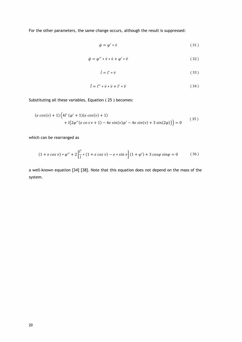
Figure 4.2.1.3 Tether logarithmic ratio for different eccentricities for 𝜑0 = 2

Figure 4.2.1.4 Tether logarithmic ratio for different eccentricities for 𝜑0 = 3

Further simulations are presented in Annex 2. Note the similarity of the first case, 𝜑0 = 0, with

the linear case for 𝜔 = 0, as it is an equivalent equation.

35

In the case of permanent orientation for values 𝜈 = 𝑘 𝜋 (𝑘 as an even integer) the tether length

should change its behavior discontinuously. In this case the implementation of the control along

the whole orbit is impossible.

For an analytical solution, an approximation of 4th order using the Taylor series is also done

allowing the integration of Equation ( 43 ). Some solutions are plotted in Figures 4.2.1.5 -

4.2.1.7.

Figure 4.2.1.5 Tether logarithmic ratio approximation comparison with 𝜑0 = 0

Figure 4.2.1.6 Tether logarithmic ratio approximation comparison with 𝜑0 = 1

36

Figure 4.2.1.7 Tether logarithmic ratio approximation comparison with 𝜑0 = 3/4

As it can be seen in Figures 4.2.1.6 and 4.2.1.7, the approximation only works for [0,𝜋], since

the approximation can’t accomplish the abrupt change at 𝜈 = 𝜋. The associated error for 𝑒 =

0.04 and 𝜑0 = 1 is shown in Figure 4.2.1.8. :

Figure 4.2.1.8 Approximation error for eccentricity = 0.04

The contours can also be seen in Figures 4.2.1.9, 4.2.1.10 and 4.2.1.11, respectively, for 𝑒 =

0.1, 𝑒 = 0.3 and 𝑒 = 0.5.

37

Figure 4.2.1.9 Tether logarithmic ratio - Contour Plot for 𝑒 = 0.1

Figure 4.2.1.10 Tether logarithmic ratio - Contour Plot for 𝑒 = 0.3

38

Figure 4.2.1.11 Tether logarithmic ratio - Contour Plot for 𝑒 = 0.5

Analyzing periodicity in this case is not in question, as the error of the approximation is quite

large, as seen in Figure 4.2.1.8.

39

Chapter 5 – Stability conditions

In the following chapter, the monodromy matrix is obtained to analyze stability with respect

to small perturbations (𝛿𝜑) of the orientation angle 𝜑.

Consider the equation studied in Section 4.1:

𝜑 = 𝜔 𝜈 + 𝜑0

( 44 )

Analyzing the neighborhood of the point 𝜑0 = 0, it follows:

𝜑 = 𝜔 𝜈 + 𝛿𝜑

( 45 )

Substituting Equations ( 40 ) and ( 45 ) to Equation ( 36 ), one obtains

(1 + 𝑒 cos ν)δφ′′ + 3 sin(𝜔𝜈 + δφ)cos(𝜔𝜈 + δφ) −3(1 + 𝜔 + 𝛿𝜑′)

1 + 𝜔𝑐𝑜𝑠(𝜔𝜈)𝑠𝑖𝑛(𝜔𝜈) = 0

( 46 )

or the nonlinear equation of perturbed motion [34]. The linearized equation is obtained through

trigonometric simplifications, with the above equation being rewritten as:

(1 + 𝑒 cos ν)δφ′′ +3

2 (2 cos(2𝜔𝜈)δφ −

sin(2ων)δφ′

1 + 𝜔) = 0

( 47 )

Equation ( 47 ) is the equation in variations. It is now possible to analyze its stability using the

Floquet theory [40], as this equation is a linearized differential equation of the second order

with periodic coefficients. The linearized equation constricts this analysis to small variations

of 𝜑. Applying Floquet theory, it is necessary to find the monodromy matrix for this equation.

5.1 Monodromy Matrix

Consider now a system of equations 𝒚 = 𝐴𝒙. For the following purpose, observe the change of

variables:

𝛿𝜑 = 𝑋1

𝛿𝜑′ = 𝑋2

40

The system can be written as:

[𝑋1′

𝑋2′] = 𝐴 [

𝑋1

𝑋2]

( 48 )

[𝑋1′

𝑋2′] = [

0 1

−3𝑐𝑜𝑠(2 𝜔 𝜈)

1 + 𝑒 𝑐𝑜𝑠 𝜈

3 𝑠𝑖𝑛(2 𝜔 𝜈)

2(1 + 𝜔)(1 + 𝑒 𝑐𝑜𝑠 𝜈)

] [𝑋1

𝑋2]

( 49 )

Some steps have to be done to obtain the monodromy matrix, based on Floquet theory [40]:

1. Do a loop, where variations occur for:

a. 𝜔, from -4 to 4, and

b. 𝑒, from 0 to 1

and include the next steps.

2. Resolve the numerical ordinary differential equations, substituting firstly:

a. 𝑋1 = 0 𝑎𝑛𝑑 𝑋2 = 1

and secondly,

b. 𝑋1 = 1 𝑎𝑛𝑑 𝑋2 = 0.

Call the solutions given by a. as [𝑎1𝑎2

] and the solutions given by b. as [𝑏1𝑏2

].

3. Create a matrix 𝐵[𝜈, 𝜔, 𝑒] where the solution of 2.a. and 2.b. are as follow:

a. 𝐵 = [𝑎1 𝑎2𝑏1 𝑏2

]

4. Create the monodromy matrix M, that obeys:

a. 𝑀[𝜈, 𝜔, 𝑒] = 2 − |𝑇𝑟 𝐵|

Note that the creation of B depends on the parameters 𝜈, 𝜔, and 𝑒. The size of the matrices B

and M depends directly with the step size defined for each parameter. Here, the step size of 𝜔

and 𝑒 was chosen = 0.01. Since the stability is related with periodicity, the matrix M was plotted

below for the value 𝜈 = 2𝜋. The indicator of stability is given by the ordinate and stability

corresponds to Tr B between 0 and 2 (0 < 2 − |𝑇𝑟 𝐵| ≤ 2), where Tr B means Trace of the matrix

B. Positive values between the described boundaries correspond to the stability of the solution

(linear approximation), negative values correspond to instability and zero values correspond to

critical cases. Figures 5.1.1, 5.1.2, 5.1.3 and 5.1.4 represent matrix M, analyzing different 𝜔.

41

Figure 5.1.1 Stability Indicator for 𝜔 = {−4;−3;−2}

As it can be seen, in the case where 𝜔 = {−4;−3;−2}, stability is found for several values of

eccentricity, with 𝜔 = −3 being the value where stability corresponds to larger intervals of

eccentricities.

Fractional numbers can be seen in Figure 5.1.2.

Figure 5.1.2 Stability Indicator for 𝜔 = {3 2⁄ ; 5 2⁄ ; 7 2⁄ }

42

Figure 5.1.3 Stability Indicator for 𝜔 = 1

In the case were 𝜔 = 1 (Figure 5.1.3), stability is only found for small values of eccentricity.

Figure 5.1.4 Stability Indicator for 𝜔 = 0

At Figure 5.1.4 (𝜔 = 0), there is a constant stability, having, nonetheless, some critical points

around 𝑒 ≅ 0.25 and 𝑒 ≅ 0.75.

43

Table 1 shows stability conditions, in function of some values of 𝜔. There are intervals of 𝑒

values where stability is always met.

Table 1. Stability conditions

Stability Conditions

𝝎 Interval of stability for 𝑒

0 𝑒 𝜖 [0, 0.99]

1 𝑒 = 0.88

2 𝑒 𝜖]0, 0.55]

3 𝑒 𝜖]0, 0.09]𝑈[0.97, 0.98]

4 𝑒 𝜖]0, 0.42]

-2 𝑒 𝜖]0, 0.54]

-3 𝑒 𝜖]0, 0.78]

-4 𝑒 𝜖]0 ,0.29]𝑈[0.91, 0.93]

Precison: 2 decimal cases

Those values have been obtained independently of the other system’s parameters, like mass of

the bodies, or gravitational force.

A contour plot of the stability range in function of 𝜔 and 𝑒 can be seen in Figure 5.1.5. The

figure shows the values where stability is found and complements Table 1.

44

Figure 5.1.5 Contour Plot of the different values of stability

45

Chapter 6 - Simulations

Simulations are quite important for mission conceptualization. They allow one to verify all the

consequences of previous work. A 2D simulator has been created to verify the properties of the

system motion. To be able to explore the dynamic demonstration with control features, a free

plugin from Wolfram Mathematica, called CDF Player (http://www.wolfram.com/cdf-player/)

should be installed.

6.1 Dynamic Behavior

Some images have been taken of the simulator, and are shown below for different

cases/considerations. Short descriptions of each case are presented.

System Earth – Satellite – Ballast

Table 2. System Earth – Satellite – Ballast Properties

System Properties considered

Satellite’s mass 1000 kg

Semi-latus rectum

Geostationary: 29 422 km

Navigation: 13 822 km

Observation: 6728 km

Eccentricity 0.003

Ballast’s mass suggestion 10% satellite’s mass

In Figure 6.1.1.1 a simulation of a geostationary satellite and a counterweight (ballast) can be

seen, and a zoom on the moving points can be seen at Figure 5.1.1.2. The satellite mass is

chosen to be 1000 kg, and the ballast possesses variable mass (with a limit). The control for

choosing a geostationary, a navigation, or an observation satellite can only be seen in the

system Earth – Satellite – Ballast.

46

Figure 6.1.1.1 Geostationary Satellite Simulation with 𝑚2 = 200 𝑘𝑔, 𝑙0 = 190 𝑘𝑚, 𝜑 = 0.08𝜈 +

2.17398,𝑂𝑟𝑏𝑖𝑡 𝑛𝑢𝑚𝑏𝑒𝑟 = 2

Figure 6.1.1.2 Geostationary Satellite Simulation zoom with 𝑚2 = 200 𝑘𝑔, 𝑙0 = 190 𝑘𝑚, 𝜑 = 0.08𝜈 +

2.17398,𝑂𝑟𝑏𝑖𝑡 𝑛𝑢𝑚𝑏𝑒𝑟 = 4

47

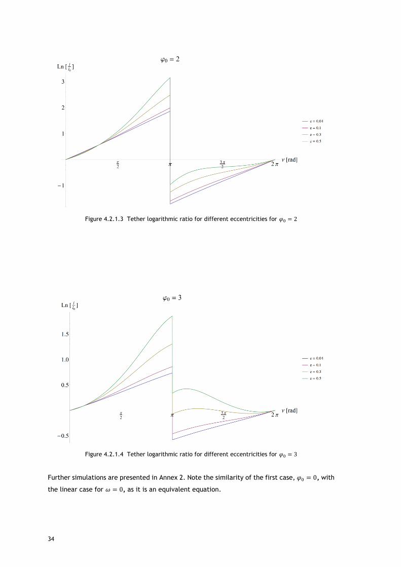
Figure 6.1.1.1 and Figure 6.1.1.2 show, in dark blue color, the mass point of the satellite, in

green the counterweight and in pink the position of the center of mass. Each point has a dashed

line that follows its motion in the same color of the respective point.

Figure 6.1.1.3 Observation Satellite Simulation with 𝑚2 = 200 𝑘𝑔, 𝑙0 = 134.56 𝑘𝑚, 𝜑 = −1.2𝜈 −

0.816814,𝑂𝑟𝑏𝑖𝑡 𝑛𝑢𝑚𝑏𝑒𝑟 = 2

Figure 6.1.1.3 shows simulation for the same system from an observation orbit. It can be seen

that the tether is too long, as it crosses the Earth.

System Earth – Moon - Ballast

This system is a simplification of the Space Elevator. For a Moon Space Elevator, it should be

remembered that the fixed angle has to be 𝜑 = 0, to allow the system to always be directed

through the Earth’s center.

48

Table 3. System Earth – Moon – Ballast Properties

System Properties considered

Moon’s mass 7.34767309 × 1022 kg

Semi-latus rectum 382843 km

Eccentricity 0.0549

Ballast’s mass suggestion 10 000 kg

The result can be seen in Figure 5.1.1.4, and shows to be an excellent solution to the Space

Elevator. A size limit for the tether is done automatically (limiting the maximum value of the

initial size 𝑙0 to 20% of the semi-latus rectum), to obtain the best solution.

Figure 6.1.2 Earth – Moon - Ballast Simulation (Space Elevator) with 𝑚2 = 10 000 𝑘𝑔, 𝑙0 = 20% semi −

latus − rectum, 𝜑 = 0, 𝑂𝑟𝑏𝑖𝑡 𝑛𝑢𝑚𝑏𝑒𝑟 = 15

49

System Earth – ISS - Space Module

In this case, the International Space Station (ISS) and a (fictitious) Space Module are simulated

(Figure 6.1.3.1). The properties of the system are represented in Table 4.

Table 4. System Earth – ISS – Space Module Properties

System Properties considered

ISS’s mass 50 000 kg

Semi-latus rectum 6799 km

Eccentricity 0.0004123

Ballast’s mass suggestion 1 000 kg

In this simulation it is possible to see that the center of mass is always moving in the same

path, but small position’s variations of the ISS (dark blue point) do make considerable changes

in the Space Module motion (as the green path suggests).

Figure 6.1.3.1 ISS Simulation Zoom with 𝑚2 = 3000 𝑘𝑔, 𝑙0 = 130 𝑘𝑚, 𝜑 = 0.2 𝜈 +

1.05558,𝑂𝑟𝑏𝑖𝑡 𝑛𝑢𝑚𝑏𝑒𝑟 = 2

50

Consider now the same system (Figure 6.1.3.2), but with the Space Module weighing 15 000 kg.

The non-rotating option is activated now (fixed angle) and the satellite points always to the

center of the Earth. After 20 orbits, the bodies describe the same path.

Figure 6.1.3.2 ISS Simulation with 𝑚2 = 15000 𝑘𝑔, 𝑙0 = 135.94 𝑘𝑚, 𝜑 = 0, 𝑂𝑟𝑏𝑖𝑡 𝑛𝑢𝑚𝑏𝑒𝑟 = 20

System Moon – SMART1 – Satellite

SMART 1 [41] is a satellite of ESA (European Space Agency) that orbited Moon. A simulation of

this satellite connected with another one can be seen in Figure 6.1.4.

51

Table 5. Moon – SMART1 – Satellite Properties

System Properties considered

SMART1’s mass 2130 kg

Semi-latus rectum 1838 km

Eccentricity 0.003

Ballast’s mass suggestion 1000 kg

In Figure 6.1.4, the trace of the second satellite is omitted. The simulation shows that the

parameters (like mass and tether length) of the mission SMART1 are executable.

Figure 6.1.4 SMART1 Simulation with 𝑚2 = 2130 𝑘𝑔, 𝑙0 = 129.56 𝑘𝑚, 𝜑 = 0.2𝜈 +

2.11115,𝑂𝑟𝑏𝑖𝑡 𝑛𝑢𝑚𝑏𝑒𝑟 = 2

52

System Titan – SST1 – SSTM

Two fictitious modules have been studied, namely SST1 (Space System in Titan 1) and SSTM

(Space System in Titan – Module), as seen in Figures 6.1.5.1 and 6.1.5.2.

Table 6. System Titan – SST1 – SSTM Properties

System Properties considered

SST1’s mass 2130 kg

Semi-latus rectum 3575 km

Eccentricity 0.0288

Ballast’s mass suggestion 100 kg

Although it is almost imperceptible, the variations of 𝜔 create a wave effect variation in the

system positions for this case. It can only be seen in the animation.

Figure 6.1.5.1 SST1 Simulation with 𝑚2 = 100 𝑘𝑔, 𝑙0 = 147.56 𝑘𝑚, 𝜑 = −2.02664𝜈 −

1.82007,𝑂𝑟𝑏𝑖𝑡 𝑛𝑢𝑚𝑏𝑒𝑟 = 2

53

Figure 6.1.5.2 SST1 Simulation with 𝑚2 = 100 𝑘𝑔, 𝑙0 = 147.56 𝑘𝑚, 𝜑 = 2.62574 −

1.82007,𝑂𝑟𝑏𝑖𝑡 𝑛𝑢𝑚𝑏𝑒𝑟 = 2

In all the presented simulations, the values of some parameters are chosen beforehand, but

can be changed any time. These options are helpful to analyze the system and can even serve

to understand the meaning of the stability conditions, as Chapter 5 predicts.

6.2 Tether actuating force

As it has been noted before, the only force actuating on the system is the gravitational

attraction. As Hao Wen et al. refer in [16], the force in the tether can be calculated as:

𝑇𝐹𝑜𝑟𝑐𝑒 =𝜇 ∗ 𝑚1 ∗ 𝑚2

𝑟12 ∗ 𝑟2

2 ∗𝑟2

3 − 𝑟13

𝑚1 ∗ 𝑟1 + 𝑚2 ∗ 𝑟2

( 50 )

For a numerical analysis of the influence of the gravitational force on the tether, it can be seen

as a function of 𝜈 (Figures 6.2.1, 6.2.2, and 6.2.3).

54

Figure 6.2.1 Earth – Satellite – Ballast variation force in function of 𝜈 for 𝑚2 = 200 𝑘𝑔, 𝑙0 =

130 𝑘𝑚, 𝜑 = 0.2ν + 0.2, 𝑂𝑟𝑏𝑖𝑡 𝑛𝑢𝑚𝑏𝑒𝑟 = 4

As Figure 6.2.1 shows, the force is small, which corresponds to the expectations, as the two-

body masses are small. For the ISS system, for example, considering a space module of 10 000

kg, the force actuating in the tether is seen in Figure 6.2.2:

Figure 6.2.2 Earth – ISS – Space Module with 𝑚2 = 10 000 𝑘𝑔, 𝑙0 = 130 𝑘𝑚, 𝜑 = 0.2ν +

0.2, 𝑂𝑟𝑏𝑖𝑡 𝑛𝑢𝑚𝑏𝑒𝑟 = 4

55

The maximum value of the tether force appears at 𝜈 = 9.54 𝜋, and reaching 46.15 N

(compression). In every simulation, increasing the initial size of the tether and/or the mass of

the second body will increase the order of values of the force actuating on the tether. The

parameters chosen for 𝜑 also change the force values, as can be seen in Figure 6.2.3:

Figure 6.2.3 Earth – ISS – Space Module with 𝑚2 = 10 000 𝑘𝑔, 𝑙0 = 130 𝑘𝑚, 𝜑 = 0.94ν +

0.0628319,𝑂𝑟𝑏𝑖𝑡 𝑛𝑢𝑚𝑏𝑒𝑟 = 4

This means that the control law of 𝜑 has a direct impact on the forces applied to the tether.

6.3 Energy analysis

Analysis of the energy balance allows one to perform the global analysis of the system. The

kinetic and potential energies can be seen in Figure 6.3.1 and Figure 6.3.2.

56

Figure 6.3.1 Kinetic energy for System Earth – ISS – Space Module with 𝑚2 = 10 000 𝑘𝑔, 𝑙0 =

130 𝑘𝑚, 𝜑 = 0.2ν + 0.2, 𝑂𝑟𝑏𝑖𝑡 𝑛𝑢𝑚𝑏𝑒𝑟 = 8

Figure 6.3.2 Potential energy for System Earth – ISS – Space Module with 𝑚2 = 10 000 𝑘𝑔, 𝑙0 =

130 𝑘𝑚, 𝜑 = 0.2ν + 0.2, 𝑂𝑟𝑏𝑖𝑡 𝑛𝑢𝑚𝑏𝑒𝑟 = 8

Kinetic and potential energies tend to oscillate, and inverse to each one, which has been

expected, as it is a conservative system.

57

Chapter 7 – Conclusions

We consider here dynamics of a two-body tethered satellite system in an elliptic geocentric

orbit. The satellites are represented as massive points connected by a light rigid link. The

tether length is assumed to be small compared to the orbit dimensions, so the orbit of the

system center of mass is supposed to be Keplerian. To describe the system motion, we deduce

the respective Lagrangian equations. These equations are used to find the control law for the

tether length that causes some programmed attitude motion of the tethered system.

We consider two types of the programmed motion: the uniform rotations of the tether and the

permanent orientation of the tether with respect to the local vertical. Substitution of the law

of motion to the Lagrangian equation permits us to obtain the differential equation for the

control; its analytical integration is not always possible and the following study is done

combining numerical analysis and approximation.

The numerical simulations of the system dynamics show that it is possible to use changes of the

tether’s length to keep uniform rotation of the tether, as well as its permanent orientation

with respect to the local vertical. The only exception is the case of 𝜔 = −1 that corresponds

to a fixed orientation of the tether in the absolute space. For all other values of the tether’s

angular velocities, including the case 𝜔 = 0 (a fixed orientation with respect to the local

vertical), one can find the control law 𝑙 = 𝑙(𝜈) that implements the referred motion. Such

control laws can be 2-π periodic for integral values of 𝜔; for some values the control laws are

not periodic.

For small values of eccentricity e the control law can be found analytically using the Taylor

series. The resulting closed-form solutions are rather cumbersome, but quite accurate for small

e as they practically coincide with the numerically obtained control laws.

Stability of the permanent rotations has been studied using the Floquet theory. The intervals

of eccentricity where the stability conditions hold true have been found for a number of angular

velocities.

For the permanent orientations with respect to the local vertical, it is found that the

orientation keeping along the whole orbit is possible only for some specific values of the

orientation angle 𝜑, e.g., for 𝜑 = 0. For other configurations, the control laws are

discontinuous making it impossible to implement the respective motion at least at a part of the

orbit.

To provide the visualization of the obtained results and to facilitate the perception of the

system dynamics, a numerical simulator of the tethered connected system has been

implemented using the Mathematica 9 software. The simulations performed using this tool

58

confirm the previously obtained results. In addition, several tethered system with realistic

parameters have been simulated and their dynamics studied and visualized.

The analysis presented here show a number of important properties of two-body tethered

systems. However, it is based on a simplified model that neglects the mass of the tether and

its flexibility and elasticity, as well as several perturbations, such as aerodynamics forces and

solar pressure. The future work should implement a more realistic system model. The other

possible direction of the research is connected with the analysis of large-scale tether system

dynamics, when the orbital motion of the system cannot be separated from its attitude

dynamics.

59

Bibliography

[1] V. Kaithi, "Design of Space Elevator," Texas, 2008.

[2] J. Arneson, "Konstantin Tsiolkovsky," March 2007. [Online]. Available: http://www.thelivingmoon.com/45jack_files/03files/Tsiolkovsky_001_Intro.html. [Accessed 14 September 2013].

[3] C. W. Swan and P. A. Swan, "Why we need a space elevator," Space Policy, vol. 22, pp. 86-91, April 2006.

[4] G. Dvorsky, "Why we'll probably never build a space elevator," February 2013. [Online]. Available: http://io9.com/5984371/why-well-probably-never-build-a-space-elevator. [Accessed 13 September 2013].

[5] B. C. Edwards and E. A. Westling, The Space Elevator: A Revolutionary Earth-to-Space Transportation System, BC Edwards, 2003.

[6] V. V. Beletsky and E. M. Levin, Dynamics of space tether systems, vol. 83, American Astronautical Society, 1993.

[7] M. P. Cartmell and D. J. McKenzie, "A review of space tether research," Progress in Aerospace Sciences, vol. 44, pp. 1-21, November 2008.

[8] M. L. Cosmo and E. C. Lorenzini, Tethers in Space Handbook, Cambridge, Massachusetts: Smithsonian Astrophysical Observatory, 1997.

[9] M. v. Pelt, Space tethers and space elevators, Springer, Ed., Copernicus Books, 2009.

[10] J. H. Hoffman, A. Mazzoleni and A. Santangelo, Design of an Artificial Gravity Generating Tethered Satellite System, New Mexico: American Institute of Physics, 2001.

[11] N/A, "Nasa Science Missions," NASA, [Online]. Available: http://science.nasa.gov/missions/tss/. [Accessed 23 February 2014].

[12] K. Fluegel, "Johnson Space Center," NASA, 25 June 1993. [Online]. Available: http://www.nasa.gov/centers/johnson/news/releases/1993_1995/93-049.html. [Accessed 23 February 2014].

[13] Y. Chen, R. Huang, X. Ren, L. He and Y. He, "History of the Tether Concept and Tether Missions: A Review," ISRN Astronomy and Astrophysics, vol. 2013, 16 January 2013.

[14] G. Zhai and Z. Jing-rui, "Space Tether Net System for Debris Capture and Remov l," in 4th International Conference on Intelligent Human-Machine Systems and Cybernetics, Nanchang, China, 2012.

[15] O. L. d. Weck, "Attitude Determination and Control (ADCS)," 2001. [Online]. Available: http://ocw.mit.edu/courses/aeronautics-and-astronautics/16-851-satellite-engineering-fall-2003/lecture-notes/l9_acs.pdf. [Accessed 11 February 2013].

[16] H. Wen, D. P. Jin and H. Y. Hu, "Advances in dynamics and control of tethered satellite systems," Acta Mech Sin, vol. 24, pp. 229-241, 2008.

[17] J. Ashenberg and E. C. Lorenzini, "Active gravity-gradient stabilization of a satellite in elliptic orits," Acta Astronautica, vol. 45, no. 10, pp. 619-627, March 1999.

[18] M. Pascal, A. Djebli and L. E. Bakkali, "Laws of deployment/retrieval in tether connected satellites systems," Acta Astronautica, vol. 45, no. 2, pp. 61-73, 1999.

[19] M. Pascal, "On fast retrieval laws for tethered satellite systems," Acta Astronautica, vol. 50, no. 8, p. 461–470, 2002.

[20] B. C. Edwards, "The Space Elevator," NASA Institute for Advanced Concepts, 2000.

[21] A. Djebl and M. Pascal, "A new method for the orbital modification of a tether connected satellite system," Acta Mechanica, vol. 167, pp. 113-122, 2004.

[22] J. Pekka, J.-P. Lebreton, S. Merikallio, M. Paton, G. Mengali and A. A. Quarta.

[23] A. Pukniel, V. Coverstone, R. Burton and D. Carroll, "The dynamics and control of the CubeSail mission: A solar sailing demonstration," Advances in Space Research, vol. 48, pp. 1902-1910, 2011.

[24] A. K. Misra, Z. Amier and V. J. Modi, "Attitude dynamics of three-body tethered systems," Acta Astronautica, vol. 17, no. 10, pp. 1059-1068, 1988.

[25] K. Kumar and K. D. Kumar, "Tethered dual spacecraft configuration: a solution to attitude control problems," Aerospace Science and Technology, vol. 4, pp. 495-505, 2000.

[26] A. D. Guerman, "Equilibria of multibody chain in orbit plane," Jorunal of Guidance, Control and Dynamics, vol. 26, no. 6, pp. 942-948, 2003.

60

[27] A. D. Guerman, "Spatial equilibria of multibody chain in a circular orbit," Acta Astronautica, vol. 58, no. 1, pp. 1-14, 2006.

[28] A. D. Guerman, "Stationary configurations of tetrahedral tethered satellite formation," Journal of Guidance, Control and Dynamics, vol. 31, no. 2, pp. 424-428, 2008.

[29] S. Yu, "Tethered Satellite System Analysis (1) - two-dimensional case and regular dynamics," Acta Astronautica, vol. 47, no. 12, pp. 849-858, 2000.

[30] A. K. Misra, "Dynamics and control of tethered satellite systems," Acta Astronautica, vol. 63, pp. 1169-1177, 2008.

[31] W. Dittrich and M. Reuter, "Poincaré Surface of Sections, Mappings," in Classical and Quantum Dynamics, Springer, 1994, pp. 155-163.

[32] A. A. Burov, I. I. Kosenko and A. D. Guerman, "Dynamics of a moon-anchored tether with variable length," Advances in the Astronautical Sciences, vol. 142, pp. 3495-3507, 2012.

[33] W. Zhang and M. H. Yao, "Periodic solutions and stability of a tethered satellite system," Mecahnics Research Communications - Elsevier, vol. 44, pp. 24-29, 2012.

[34] A. A. Burov, I. I. Kosenko and A. D. Guerman, "Uniform rotations of a two-body tethered system in an elliptic orbit," in 64th International Astrounautical Congress, Beijing, China, 2013.

[35] H. D. Curtis, Orbital Mechanics for Engineering Students, Daytona Beach, Florida: Elsevier, 2010.

[36] A. D. Guerman, Dinâmica dos Sistemas Mecânicos - 1. Métodos da mecânica analítica, Covilhã, 2002.

[37] J. A. Shapiro, Classical Mechanics, 2010.

[38] A. A. Burov, "Oscillations of a Vibrating Dumbbell on an Elliptic Orbit," Doklady Physics, vol. 56, no. 3, pp. 182-185, 2011.

[39] A. A. Burov, A. D. Guerman and I. I. Kosenko, "Dynamics of tethered system connected to moon surface," in DyCoSS - 2nd IAA Conference on Dynamics and Control of Space Systems, Rome, 2014.

[40] J. Yang, "Basic Floquet Theory," 2011. [Online]. Available: http://www.emba.uvm.edu/~jxyang/teaching/Floquet_theory_Ward.pdf. [Accessed 12 June 2014].

[41] D. P. S. d. Santos, A. B. Prado, L. Casalino and G. Colasurdo, "Optimal trajectories using gravity assisted maneuver and solar electric propulsion (SEP) towards near-earth-objects," Journal of Aerospace Engineering, vol. 1, no. 2, p. 51, 2008.

[42] M. Navabi, N. Nasiri and M. Dehghan, "Modeling and numerical simulation of linear and nonlinear spacecraft attitude dynamics and gravity gradient moments: A comparative study," Commun Nonlinear Sci Numer Simulat, vol. 17, pp. 1065-1084, 2012.

61

Annex 1

In Section 2.3 were presented some applications and mission of satellite tether systems. Here,

a complete list is shown of important missions (with or without succeeded status).

Table 7. TSS missions till 2013

Mission Year Sponsor Orbit Length Status

Gemini XI 1967 NASA LEO 50 m Launched

Gemini XII 1967 NASA LEO 30 m Launched

TPE-1 1980 NASA/ISAS Suborbital 400 m Launched

TPE-2 1981 NASA/ISAS Suborbital 500 m Launched

TPE-3 (CHARGE-1) 1983 NASA/ISAS Suborbital 500 m Launched

CHARGE-2 1985 NASA/ISAS Suborbital 500 m Launched

MAIMIK 1986 NASA/NDRE LEO 400 m Launched

ECHO-7 1988 USAF Suborbital — Launched

OEDIPUS-A 1989 NRC/NASA/CRC/CSA Suborbital 958 m Launched

CHARGE-2B 1992 NASA/ISAS Suborbital 500 m Launched

TSS-1 (STS-46) 1992 NASA/ASI LEO 267 m Launched

SEDS-1 1993 NASA LEO 20 m Launched

PMG 1993 NASA LEO 500 m Launched

SEDS-2 1994 NASA LEO 20 m Launched

OEDIPUS-C 1995 NASA/NRC/CRC/CSA Suborbital 1 km Launched

62

TSS-1R (STS-75) 1996 NASA/ASI LEO 19.6 km Launched

TSS-2 (STS-75) 1996 NASA LEO 100 m Cancelled

TiPS 1996 NRO/NRL LEO 4 km Launched

YES 1997 ESA/Delta-Utec LEO 35 m Launched

ATEx 1999 NRO/NRL LEO 22 m Launched

PICOSATs 2000 Aerospace

corporation LEO 30 m Launched

MEPSI 2002 Aerospace

corporation LEO 15.2 m Launched

ProSEDS 2003 NASA LEO 15 m Cancelled

MAST 2007 NASA/TUI/Stanford LEO 1 km Launched

YES2 2007 ESA/Delta-Utec LEO 31.7 m Launched

STARS 2009 Kagawa university LEO 5 m Launched

T-REX 2010 ISAS/JAXA LEO 300 m Launched

TEPCE 2013 NRO/NRL LEO 1 km Planning

63

Annex 2

In Chapter 4 an analysis was done for 𝜑 control laws. The graphics of other simulations done

can be seen in the present annex. The following graphics were obtained with the previous

substitution of 𝜔 and consequent integration.

2.1 Uniform rotations

Figure A.2.1 Tether logarithmic ratio for different eccentricities and 𝜔 = 1/4

Figure A.2.2 Tether logarithmic ratio for different eccentricities and 𝜔 = 1/2

64

Figure A.2.3 Tether logarithmic ratio for different eccentricities and 𝜔 = −3

Figure A.2.4 Tether logarithmic ratio for different eccentricities and 𝜔 = −2

65

Figure A.2.5 Tether logarithmic ratio for different eccentricities and 𝜔 = −1/4

Figure A.2.6 Tether logarithmic ratio for different eccentricities and 𝜔 = −1/2

66

Figure A.2. 7 Tether logarithmic ratio for different eccentricities and 𝜔 = −3/4

Figure A.2. 8 Tether logarithmic ratio for different eccentricities and 𝜔 = −5/4

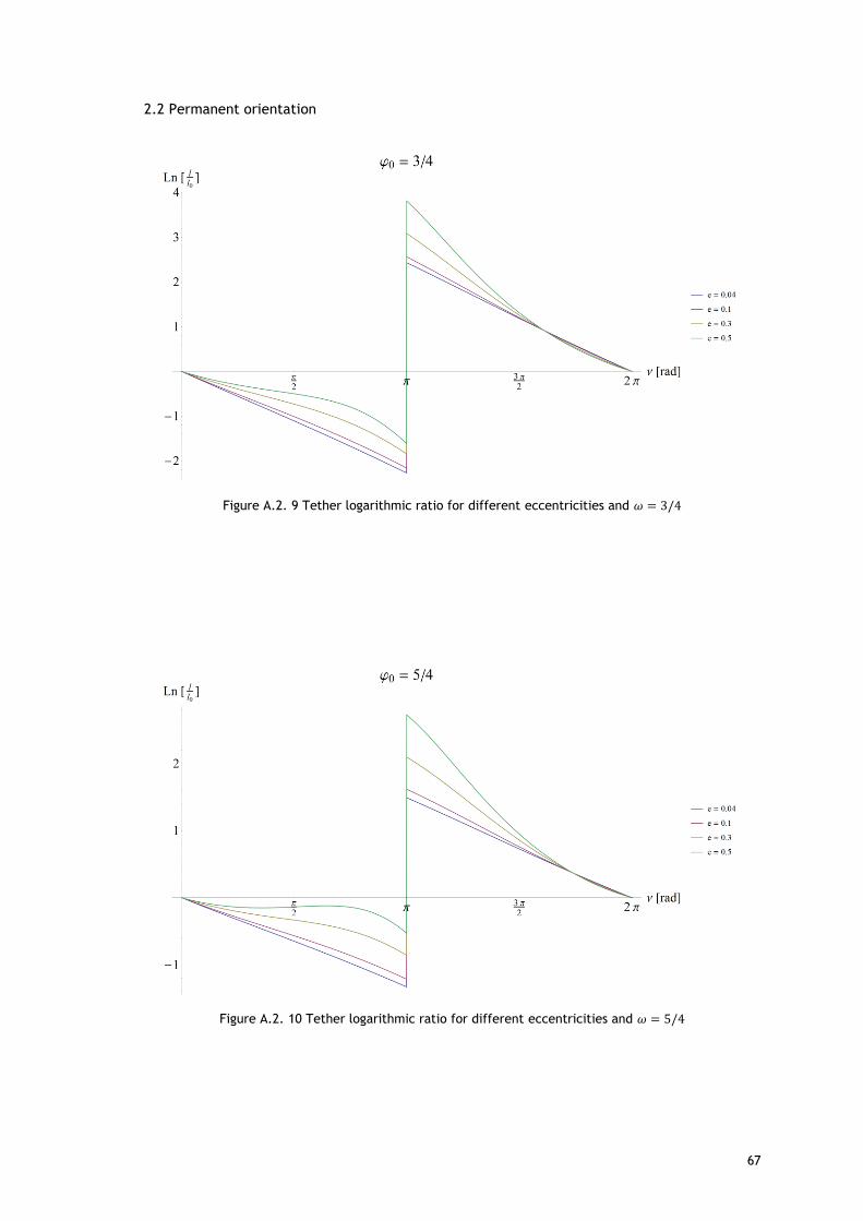
67

2.2 Permanent orientation

Figure A.2. 9 Tether logarithmic ratio for different eccentricities and 𝜔 = 3/4

Figure A.2. 10 Tether logarithmic ratio for different eccentricities and 𝜔 = 5/4

68

Figure A.2. 11 Tether logarithmic ratio for different eccentricities and 𝜔 = −3

Figure A.2. 12 Tether logarithmic ratio for different eccentricities and 𝜔 = −2

69

Figure A.2. 13 Tether logarithmic ratio for different eccentricities and 𝜔 = −3/4

Figure A.2. 14 Tether logarithmic ratio for different eccentricities and 𝜔 = −5/4