Embed Size (px)
Citation preview
UNIVERSIDADE DE LISBOA FACULDADE DE CIÊNCIAS
DEPARTAMENTO DE FÍSICA
ANALYSIS OF THE EXTRATROPICAL
STRATOSPHERE-TROPOSPHERE CIRCULATION
COUPLING USING A 3D NORMAL MODE APPROACH
Margarida da Conceição Rasteiro Magano Lopes Rodrigues Liberato
DOUTORAMENTO EM FÍSICA
(Meteorologia)
2008


UNIVERSIDADE DE LISBOA FACULDADE DE CIÊNCIAS
DEPARTAMENTO DE FÍSICA
ANALYSIS OF THE EXTRATROPICAL
STRATOSPHERE-TROPOSPHERE CIRCULATION
COUPLING USING A 3D NORMAL MODE APPROACH
Margarida da Conceição Rasteiro Magano Lopes Rodrigues Liberato
DOUTORAMENTO EM FÍSICA
(Meteorologia)
Tese orientada pelo Professor Doutor Carlos da Camara, Professor Associado do Departamento de Física da Faculdade de Ciências da Universidade de Lisboa e pelo Professor Doutor José Manuel Castanheira, Professor Auxiliar do Departamento de Física da
Universidade de Aveiro
2008


i
ACKNOWLEDGEMENTS
First of all, I would like to thank my supervisors. I am especially indebted to Prof.
José Manuel Castanheira for introducing me to the 3D Normal Modes enchanted,
though physically based, world. I am grateful for his guidance, his enthusiasm, his
neverending persistence, confidence and patience as well as for all his suggestions for
further research. Without his constructive support and encouragement, friendship and
advice this thesis would not have been finished. I am especially grateful to Prof.
Carlos da Camara for suggesting this research theme and for being my supervisor, for
his advice and support as well as for his friendship.
I am also extremely thankful to my friend and PhD colleague, Célia Gouveia for her
unconditional friendship and endless patience and support, share of information,
valuable suggestions and fruitful scientific discussions, which helped overcoming
difficulties and broadened my scientific interests and research. I am also thankful to
Dr. Ricardo Trigo for his friendship and support, words of motivation, suggestions,
share of information as well as enthusiastic and varied conversations, some science-
related, many not, contributing to make each visit to FCUL a gratifying experience.
I am thankful to the University of Trás-os-Montes e Alto Douro, where I have been
teaching since 1998, for granting a three-year leave for full time scientific research,
and for allowing my participation at all the International Scientific Conferences and
Symposiums where I have presented scientific results. A word of recognition and
acknowledgment is also due to my colleagues at the Physics Department for support
that eased the last several years and made work a more enjoyable experience.

ii
Finally, a very special thought towards my family and close friends, for the love they
have always demonstrated, for their neverending patience, support and
encouragement. To my husband, José António, who provided more love and support
than anyone could deserve, and to my daughters, Catarina and Helena, I dedicate this
work.
The Portuguese Foundation of Science and Technology (FCT) partially supported this
research (Grant SFRH / BD / 32640 / 2006).

iii
ABSTRACT
The annular nature of the leading patterns of the Northern Hemisphere winter
extratropical circulation variability is analysed by means of a Principal Component
Analysis (PCA) of tropospheric geopotential height fields followed by lagged
correlations of relevant Principal Components with the stratospheric polar vortex
strength as well as with a proxy of midlatitude tropospheric zonal mean zonal
momentum anomalies.
Results suggest that two processes, occurring with a time scale separation of about
two weeks, contribute for the Northern Annular Mode (NAM) spatial structure. Polar
vortex anomalies appear to be associated with midlatitude tropospheric zonal
momentum anomalies leading the vortex. Zonal mean zonal wind anomalies of the
same sign lagging the vortex are then observed in the troposphere at high latitudes.
Tropospheric variability patterns which seem to respond to the polar vortex variability
have a hemispheric scale. A dipolar structure may be observed only over the Atlantic
basin that resembles the North Atlantic Oscillation pattern (NAO), but with the node
line shifted northward.
The association between zonal symmetric components of the tropospheric and
stratospheric circulations is further confirmed by a PCA on the barotopic component
of the Northern winter atmospheric circulation. Results show that a zonally
symmetric component of the middle and lower tropospheric circulation variability
exists at high latitudes. At the middle latitudes obtained results suggest that the
zonally symmetric component, as identified in other works, is artificially
overemphasized by the usage of PCA on single isobaric tropospheric levels.
The 3-Dimensional normal mode expansion of the atmospheric general circulation
was also used to relate the variability of the stratospheric polar vortex to the energy
variability of the forcing planetary waves. Positive (negative) anomalies of the energy

iv
associated with the first two baroclinic modes of planetary Rossby waves with zonal
wavenumber 1 are followed by downward progression of negative (positive)
anomalies of the vortex strength. The analysis of the correlations between individual
Rossby modes and the vortex strength further contributed to confirm the result from
linear theory that the waves which force the vortex are those associated with the
largest zonal and meridional scales.
Keywords: stratospheric polar vortex; wave-mean flow interaction; Northern Annular
Mode; Artic Oscillation; North Atlantic Oscillation; 3D normal mode; planetary or
Rossby waves; Stratospheric Sudden Warming and Stratospheric Final Warming.

v
RESUMO
Nas últimas décadas assistiu-se a um interesse crescente pelo estudo da interacção
entre a troposfera e a estratosfera extratropicais. A atenção dedicada a este tema
justifica-se, em boa parte, pela relação existente entre a variabilidade estratosférica e
os modos anulares na troposfera. Cada vez mais se tem maior evidência de que os
processos dinâmicos na estratosfera desempenham um papel significativo na
variabilidade climática da troposfera através de uma larga gama de escalas temporais.
Com efeito, as relações estatísticas entre a intensidade do vórtice polar e a circulação
troposférica estendem-se até à superfície, podendo tornar-se úteis para a previsão do
tempo à escala mensal [Baldwin e Dunkerton 2001], bem como para uma melhor
compreensão da variabilidade climática.
O acoplamento dinâmico estratosfera-troposfera tem influência na variabilidade
climática da circulação troposférica [Perlwitz e Graf 1995; Thompson e Wallace
1998; Castanheira e Graf 2003], tendo Perlwitz e Graf [1995] mostrado que anomalias
da circulação estratosférica exercem influência sobre os regimes de circulação da
troposfera e posteriormente sugerido que a reflexão de ondas planetárias
desempenhava papel importante [Perlwitz e Graf 2001a]. Outros autores [Hines 1974;
Geller e Alpert 1980; Schmitz e Grieger 1980; Perlwitz e Harnik 2003] têm
igualmente sugerido a reflexão descendente da energia das ondas pela estratosfera de
volta à troposfera como constituindo um mecanismo pelo qual a estratosfera pode
afectar a troposfera.
Nas latitudes elevadas do Hemisfério Norte, a variabilidade da estratosfera é
dominada por intensificações e desacelerações “esporádicas” do vórtice polar, que
ocorrem com escalas temporais da ordem de semanas a meses durante o Inverno
[Holton e Mass 1976; Yoden 1990; Scott e Haynes 1998]. O forçamento troposférico
da variabilidade estratosférica é então explicado pela propagação vertical de ondas,
que transferem momento e energia para a estratosfera. Contudo, os mecanismos
vi
dinâmicos pelos quais a troposfera reage a variações da estratosfera não estão ainda
bem compreendidos. Muitos estudos recentes do acoplamento dinâmico entre a
estratosfera e a troposfera enfatizam a dinâmica do escoamento médio zonal
relacionada com os Modos Anulares [Baldwin e Dunkerton 1999; 2001; Kuroda e
Kodera 1999; Kodera et al. 2000; Christiansen 2001; Ambaum e Hoskins 2002; Black
2002; Polvani e Kushner 2002; Plumb e Semeniuk 2003]. Acresce que as
observações, em particular, mostram que anomalias elevadas na intensidade do
vórtice polar estratosférico descem à baixa estratosfera, sendo seguidas por regimes
meteorológicos troposféricos anómalos semelhantes ao Modo Anular do Hemisfério
Norte (NAM) [Baldwin e Dunkerton 1999; 2001; Thompson et al. 2002].
O fenómeno de aquecimento súbito estratosférico (SSWs - Sudden Stratospheric
Warmings) domina a variabilidade da circulação estratosférica durante o Inverno do
Hemisfério Norte, tendo-se que os SSWs envolvem interacções entre o escoamento
zonal da estratosfera polar e as ondas planetárias de propagação ascendente,
principalmente com números de onda zonal 1 e 2 [Andrews et al. 1987]. Durante um
SSW as temperaturas estratosféricas polares aumentam e o escoamento médio zonal
enfraquece dramaticamente num curto intervalo de tempo. Com este enfraquecimento
do escoamento zonal, a circulação estratosférica torna-se extremamente assimétrica e
o vórtice estratosférico polar é afastado do pólo. Nos casos mais dramáticos, as
temperaturas podem subir cerca de 50 K, e o escoamento estratosférico circumpolar
pode reverter em apenas alguns dias [Limpasuvan et al. 2004].
Nesta conformidade, procede-se ao estudo da natureza anular dos principais padrões
de variabilidade da circulação extratropical durante o Inverno do Hemisfério Norte e
apresentam-se resultados que evidenciam a separação entre as componentes anular e
não anular da variabilidade da circulação atmosférica do Hemisfério Norte. Efectua-se
uma Análise em Componentes Principais dos campos troposféricos da altura do
geopotencial, procedendo-se, em seguida, a um estudo das correlações desfasadas das
Componentes Principais relevantes com a intensidade do vórtice polar estratosférico e
com um proxy das anomalias das médias zonais do vento zonal nas latitudes médias

vii
da troposfera. Os dados utilizados consistem em reanálises do European Centre for
Medium-Range Weather Forecasts (ECMWF ERA-40) [Uppala et al. 2005]
Os resultados sugerem que os processos, que contribuem para a estrutura espacial do
NAM, ocorrem em duas fases distintas, separadas por cerca de duas semanas.
Anomalias das médias zonais do vento zonal nas latitudes médias da troposfera
precedem, em cerca de uma semana, anomalias, de igual sinal, na intensidade do
vórtice polar. Posteriormente às anomalias do vórtice polar, observam-se anomalias,
de igual sinal, no vento médio zonal, na troposfera em latitudes elevadas. Estes
resultados sugerem, pois, que o padrão dominante da variabilidade troposférica (o
NAM), abundantemente referido na literatura, representa variabilidade associada a
uma mistura de processos desfasados no tempo. Os padrões de variabilidade
troposféria, que surgem como resposta à variabilidade do jacto polar boreal,
apresentam uma escala hemisférica embora contenham uma estrutura dipolar,
localizada apenas sobre a bacia Atlântica. Embora esse dipolo se assemelhe ao padrão
da NAO, a linha nodal surge deslocada para Norte.
A natureza dinâmica da AO e da NAO é ainda investigada através de uma nova
abordagem que combina os métodos tradicionais multivariados, como a Análise em
Componentes Principais, com um procedimento de filtragem dinâmica baseado na
análise tridimensional de modos normais da circulação global da atmosfera, cuja
utilização se justifica na medida em que proporciona uma filtragem dos dados
determinada pela própria natureza termohidrodinâmica do escoamento atmosférico.
Com efeito, para além da decomposição da análise de Fourier em número de onda
zonal, o esquema de modos normais permite ainda uma separação nas escalas
espaciais meridional e vertical e, sobretudo, assegura uma decomposição do campo da
circulação nas suas componentes rotacional e divergente. Os dados utilizados
consistem em reanálises do National Centers for Environmental Prediction–National
Center for Atmospheric Research (NCEP-NCAR; Kalnay et al. 1996; Kistler et al.
2001). Analisam-se as variabilidades anular e não anular da circulação extratropical
durante o Inverno do Hemisfério Norte, tendo-se que os resultados obtidos mostram

viii
que metade da variabilidade mensal da circulação barotrópica, com simetria zonal, do
Hemisfério Norte, representada pela primeira EOF, é estatisticamente distinta da
variabilidade remanescente. A correlação dos índices NAM da baixa estratosfera com
as séries temporais diárias das anomalias da circulação projectadas sobre a primeira
EOF é elevada (r > 0.7), evidenciando o facto de que a variabilidade anular se estende
desde a estratosfera até à troposfera.
A realização de uma Análise em Componentes Principais à variabilidade residual do
campo da altura do geopotencial aos 500-hPa – definida como a variabilidade
remanescente após subtracção do campo da altura do geopotencial aos 500-hPa
projectado sobre o índice NAM da baixa estratosfera – revela também um padrão com
uma componente zonalmente simétrica nas latitudes médias. Contudo, esta
componente zonalmente simétrica surge na segunda EOF da variabilidade residual e
corresponde a dois dipolos independentes sobre os oceanos Pacífico e Atlântico. Estes
resultados evidenciam a existência, nas latitudes elevadas, de uma componente
zonalmente simétrica da variabilidade da circulação da baixa e média troposferas. Nas
latitudes médias, a componente zonalmente simétrica da variabilidade da circulação –
a existir – é, pois, artificialmente enfatizada pela utilização da Análise em
Componentes Principais em níveis isobáricos troposféricos únicos.
O acoplamento dinâmico estratosfera-troposfera foi também estudado através da
análise da energia associada às ondas planetárias. A expansão em modos normais
tridimensionais da circulação geral da atmosfera proporciona a separação da energia
total (cinética + potencial disponível) da atmosfera entre energia associada a ondas
planetárias ou de Rossby e a ondas gravítico-inerciais, com estruturas verticais
barotrópica ou baroclínicas. A análise, aqui efectuada, distingue-se das análises
tradicionais, pois o forçamento estratosférico é diagnosticado em termos das
anomalias da energia total associada a ondas tridimensionais, em vez das anomalias
dos fluxos de calor e de momento associados a componentes de Fourier obtidas
através de uma decomposição unidimensional da circulação atmosférica.

ix
No contexto da dinâmica da interacção entre as ondas e o escoamento médio e através
do estudo das correlações desfasadas entre a intensidade do jacto polar e a energia das
ondas, investigou-se a forma como o vórtice polar oscila em função da energia total
das ondas de Rossby. Foi também analisada a forma como ambas as escalas, zonal e
meridional, dos modos de Rossby interagem com a intensidade do vórtice. Os
resultados indicam que um aumento da energia total é acompanhado por um aumento
da propagação de ondas de número de onda zonal 1 para a estratosfera, que
desaceleram o jacto. A análise da correlação entre os modos de Rossby individuais e a
intensidade do vórtice confirmam ainda os resultados da teoria linear que indicam que
as ondas que forçam o vórtice polar são as associadas com as maiores escalas zonal e
meridional.
Finalmente, efectuaram-se análises de compósitos aos dois tipos de fenómenos de
aquecimento súbito estratosférico, nomeadamente aos episódios ditos de
deslocamento e de separação, tendo os respectivos compósitos revelado que se
encontram associados a mecanismos dinâmicos distintos. Mostra-se que os fenómenos
de aquecimento súbito estratosférico do tipo deslocamento são forçados por anomalias
positivas da energia, associadas com os dois primeiros modos baroclínicos das ondas
planetárias de Rossby com número de onda zonal 1. Por outro lado, os fenómenos de
aquecimento súbito estratosférico do tipo separação são forçados por anomalias
positivas da energia, associadas com as ondas planetárias de Rossby com número de
onda zonal 2, surgindo o modo barotrópico como a componente mais importante. De
referir, finalmente, que no que respeita aos fenómenos de aquecimento final
estratosférico, os resultados obtidos sugerem que o mecanismo dinâmico é semelhante
ao dos fenómenos de aquecimento súbito estratosférico do tipo deslocamento.
Palavras Chave: vórtice polar estratosférico; interacção entre ondas e escoamento
médio; modo anular; NAO e AO; modos normais 3D; ondas planetárias ou de
Rossby; aquecimento súbito estratosférico.

xi
TABLE OF CONTENTS
ACKNOWLEDGEMENTS............................................................................................i
ABSTRACT................................................................................................................. iii
RESUMO.......................................................................................................................v
TABLE OF CONTENTS..............................................................................................xi
LIST OF FIGURES .....................................................................................................xv
LIST OF TABLES................................................................................................... xxiii
LIST OF ACRONYMS .............................................................................................xxv
1. INTRODUCTION .....................................................................................................1
2. THEORETICAL BACKGROUND...........................................................................5
2.1. Waves in the atmosphere ....................................................................................5
2.2. Zonal mean dynamical structure of the atmosphere ...........................................5
2.3. Planetary or Rossby waves and stratospheric vortex dynamics..........................9
3. DATA AND METHODS ........................................................................................15
3.1. Three-dimensional Normal Mode Decomposition ...........................................16
3.1.1. 3D Normal Mode Decomposition Scheme................................................18
3.2. Principal Component Analysis .........................................................................21
3.2.1. PCA on filtered transformed space ............................................................23
3.2.2. On the physical meaning of EOFs .............................................................25
3.3. Data and Data Preparation ................................................................................27

xii
3.3.1. Projection onto 3D normal modes .............................................................27
3.3.2. PCA............................................................................................................29
3.3.3. Stratospheric Polar Vortex Strength Indices..............................................29
3.3.4. Midwinter Sudden Warming Events..........................................................29
3.3.5. Stratospheric Final Warming Events .........................................................33
3.3.6. Climatology and Anomalies ......................................................................34
3.3.7. Statistical Significance of Anomalies ........................................................34
4. BRIDGING THE ANNULAR MODE AND NORTH ATLANTIC
OSCILLATION PARADIGMS...................................................................................37
4.1. Extratropical Atmospheric Circulation Variability...........................................38
4.1.1. Space-time variability of horizontal circulation ........................................38
4.1.1.1. NH winter season teleconnection patterns..........................................40
4.1.1.2. AO and Annular Modes ......................................................................46
4.1.2. Vertical Coupling.......................................................................................49
4.1.3. NAO and NAM paradigms ........................................................................53
4.1.4. The Timescale of teleconnection patterns..................................................57
4.2. Principal Component Analysis .........................................................................59
4.2.1. Extratropical tropospheric circulation variability ......................................60
4.2.2. Stratospheric-Tropospheric connection .....................................................62
4.2.3. Variability linearly decoupled from the midlatitude zonal mean zonal
wind......................................................................................................................68
4.2.3.1. The effect of filtering ..........................................................................74
4.3. Annular versus non-annular circulation variability ..........................................76

xiii
4.3.1. 3D normal modes dynamical filtering .......................................................76
4.3.2. Tropospheric variability decoupled from the stratosphere ........................84
4.3.2.1. 1000-hPa geopotential height field .....................................................90
5. WAVE ENERGY ASSOCIATED WITH THE VARIABILITY OF THE
STRATOSPHERIC POLAR VORTEX ......................................................................95
5.1. Energy spectra associated with climatological circulation and wave
transience .................................................................................................................96
5.1.1. Energy associated with wave transience....................................................97
5.1.2. Variability of wave energy.......................................................................100
5.2. Study of Vortex Variability – the classical approach .....................................104
5.3. Study of Vortex Variability – the energy perspective ....................................112
5.3.1. Lagged correlations between the vortex strength and the wave energy ..114
5.3.1.1. Zonal dependence .............................................................................114
5.3.1.2. Meridional dependence.....................................................................117
5.3.1.3. SSW events .......................................................................................120
5.3.2. SFW events ..............................................................................................124
6. CONCLUSIONS....................................................................................................127
REFERENCES ..........................................................................................................133


xv
LIST OF FIGURES
Figure 2.1 – Longitudinally averaged zonal component of wind in troposphere and
stratosphere for December to March (Northern Hemisphere winter). Negative
regions correspond to westward winds (contour: 5 m/s). The winter hemisphere
has strong eastward jets in the stratosphere (the “polar vortex”) while the
summer hemisphere has strong westward winds. The field is based on monthly
mean zonal wind from ECMWF (ERA-40) Reanalysis covering the period 1958-
2002........................................................................................................................6
Figure 3.1 – Vertical structure functions of the barotropic m = 0 and the first four
baroclinic modes (m = 1,…,4) of the NCEP–NCAR atmosphere. It is worth
noting that the NCEP–NCAR database only extends up to the 10-hPa level. .....28
Figure 3.2 – Polar stereographic plot of geopotential height (contours) on the 10-hPa
pressure surface. Contour interval is 0.4 km, and shading shows potential
vorticity greater than 4.0×10⁻⁶ K kg-1 m2 s-1. (a) A vortex displacement type
warming that occurred in February 1984. (b) A vortex splitting type warming
that occurred in February 1979 (Figure 1 from Charlton and Polvani [2007]). ..31
Figure 4.1 – Strongest negative correlation i
ρ on each one-point correlation map,
plotted at the base grid point (originally referred to as “teleconnectivity”) for (a)
SLP and (b) 500-hPa height. Correlation fields were computed over 45 winter
months from 1962-1963 to 1976-1977. Negative signs have been omitted and
correlation coefficients multiplied by 100. Regions where 60i
ρ < are unshaded;
60 75i
ρ≤ < stippled lightly; 75i
ρ≤ stippled heavily. Arrows connect centres of
strongest teleconnectivity with the grid point, which exhibits strongest negative
correlation on their respective one-point correlation maps (Figure 7 from
Wallace and Gutzler [1981])................................................................................41
xvi
Figure 4.2 – One-point correlation map showing correlation coefficients between SLP
at the grid point 30°N, 20°W, and SLP at every grid point. Based on same 45-
month data set as Figure 4.1. Contour interval is 0.2 (Figure 8b from Wallace
and Gutzler [1981])..............................................................................................43
Figure 4.3 – The NAO in January as depicted in the RPCA of Barnston and Livezey
[1987]...................................................................................................................43
Figure 4.4 – Monthly mean 500-hPa height and SLP fields regressed on standardized
PC1 and PC2 of monthly mean DJFM SLP anomalies poleward of 20ºN, based
on data for the period 1958–99. Contour interval 1.5 hPa for SLP and 15 m for
500-hPa height; negative contours are dashed. The latitude circles plotted
correspond to 30º and 45ºN (Figure 1 from Quadrelli and Wallace [2004b]). ....45
Figure 4.5 – Difference between the mean SLP in the two vortex regimes (SVR-
WVR). Contour interval is 0.75 mb. Negative contours are dashed and the zero
contour line has been suppressed. The shading indicates where the mean
difference is significant at least at the 95% confidence level (Figure 8 from
Castanheira and Graf [2003])...............................................................................57
Figure 4.6 – Regression patterns (EOFs) of the 1000-hPa geopotential height on
standardized PCs of 15-days running mean climatological anomalies, north of
30ºN. EOFs 1, 2 and 3 explain 19.0%, 11.8% and 10.3% of the climatological
variability, respectively. Contour interval is 10 gpm, and negative contours are
dashed. .................................................................................................................61
Figure 4.7 – As in Figure 4.6 but for 500-hPa geopotential height field. EOFs 1, 2 and
3 explain 15.1%, 11.2% and 9.8% of the total variability, respectively. Contour
interval is 15 gpm.................................................................................................61
Figure 4.8 – Meridional profiles of the zonal mean amplitude of the first (solid line)
and second (dashed line) EOFs of the 500-hPa geopotential height variability.
The amplitudes were normalized to one standard deviation of the respective
PCs. ......................................................................................................................64

xvii
Figure 4.9 – Lagged correlations between the 50-hPa zonal mean zonal wind at 65ºN
(U50 (65)) and the first two PCs of the 500-hPa geopotential height fields. The
curve U500 represents the lagged correlation between the U50 (65) index and the
500-hPa zonal mean zonal wind in the latitudinal belt 45–55ºN. The bottom
plot is similar to the top one but considering only U50 (65) anomalies above or
below one standard deviation. Positive lags mean that the stratospheric wind is
leading..................................................................................................................65
Figure 4.10 – Schematic interpretation of the correlations in Figure 4.9. ...................67
Figure 4.11 – As in Figure 4.6 but for the residual geopotential height variability.
EOFs 1, 2 and 3 explain 17.7%, 11.8% and 11.4% of the 1000-hPa residual
variability, respectively........................................................................................68
Figure 4.12 – As in Figure 4.7 but for the residual geopotential height variability.
EOFs 1, 2 and 3 explain 13.5%, 13.1% and 11.6% of the 500-hPa residual
variability, respectively........................................................................................69
Figure 4.13 – Meridional profiles of the zonal mean amplitude of the first EOF of the
residual 500-hPa geopotential height variability (solid line) and second EOF of
the total 500-hPa geopotential height variability (dashed line). The amplitudes
are normalized to one standard deviation of the respective PCs. ........................69
Figure 4.14 – Lagged correlations between the 50-hPa zonal mean zonal wind at 65ºN
and the leading PCs of the total (solid line) and residual (dashed line)
variabilities of (top) 1000-hPa and (bottom) 500-hPa geopotential height fields.
Positive lags mean that the stratospheric wind is leading....................................72
Figure 4.15 – As in Figure 4.14 but considering only 50-hPa zonal mean zonal wind
anomalies above or below one standard deviation. .............................................73
Figure 4.16 – As Figure 4.9 (bottom) but (a) considering unfiltered (i.e. not averaged)
time series and (b) considering only the intraseasonal variability. The curve
PC1res represents the lagged correlation between the U50 (65) index and the

xviii
leading PC of the 500-hPa geopotential height residual variability. ...................75
Figure 4.17 – (Top) Zonal mean meridional structures of the leading EOFs of the
barotropic circulation and of the 500-hPa geopotential height (Z500). (Bottom)
Zonal mean meridional structures of the leading EOFs of the Z500 variability
and of the Z500 variability regressed onto the 70-hPa NAM. U500 and Z500
(U500R and Z500R) denote the velocity and the 500-hPa geopotential height
(regressed on the 70-hPa NAM). U00 and Z00 denote the velocity and
geopotential height of the barotropic circulation. The structures are normalized to
one standard deviation of the respective PCs. The geopotential height and the
velocity units are respectively gpm and 10-1 × ms-1. ...........................................78
Figure 4.18 – (Top) First three EOF patterns of the 500-hPa geopotential height
variability. (Middle) Regression pattern of the Z500 field onto the 70-hPa NAM.
(Bottom) As in the top panel, but for the residual variability, i.e. the variability
that remained after subtraction of Z500 regressed on the 70-hPa NAM. The
patterns are normalized to 1 standard deviation of the respective PCs. The values
in the right top of each panel are the percentages of variance represented by each
(EOF, PC) pair. Contour interval is 10 gpm, except in the regression pattern
where the contour interval is 7.5 gpm..................................................................81
Figure 4.19 – Lagged correlations between the daily data projections onto the first
EOF of the barotropic mode and the NAM indices. Solid curves are for
stratospheric NAMs from 10-hPa (black) to 150-hPa (light gray). The dashed red
curve is for 1000-hPa NAM and the dashed blue curve is for 500-hPa NAM.
Positive lags mean that NAM indices are leading. ..............................................82
Figure 4.20 – Correlation between the zonal wind means in the longitude sectors of
[90ºE, 225ºE] and [90ºW, 30ºE]. The black curve corresponds to daily
anomalies. The blue and the red lines correspond to daily anomalies smoothed by
11-day and 31-day running means, respectively..................................................83

xix
Figure 4.21 – (Top) Zonal mean meridional structures of the first EOFs of the total
and residual Z500 variabilities. (Bottom) Zonal mean meridional structures of the
first EOFs of the total and the second EOF of the residual variability. U500R and
Z500R denote the meridional profiles of the velocity and geopotential height
associated with the EOFs of the residual variability, respectively. .....................86
Figure 4.22 – Correlation maps between Z500 residual anomalies and the four time
series defined over the Pacific (Pac.), Siberia (Sib.), Iceland (Ice.) and over the
Bering Strait (Ber.) centres (see the text for the definition of these centres).
Contour interval is 0.15. The solid thick lines represent the zero contours.........88
Figure 4.23 – As in Figure 4.18 but for the 1000-hPa geopotential height field
(Z1000). Contour interval is 5 gpm. ....................................................................91
Figure 4.24 – Correlation maps between Z1000 residual anomalies and the three
1000-hPa anomaly time series defined over the Atlantic (Atl.), Pacific (Pac.) and
Iceland (Ice.) centres (see the text for the definition of these centres). Contour
interval is 0.15. The solid thick lines represent the zero contours. ......................92
Figure 4.25 – (Top) Regression maps of the Z1000 residual anomalies on the three
normalized 1000-hPa anomaly time series defined over the Atlantic (Atl.),
Pacific (Pac.) and Iceland (Ice.) centres (see the text for the definition of these
centres). (Bottom) As in the top but regressing out also the variability associated
with the PC2. Contour interval is 5 gpm. The solid thick lines represent the zero
contours................................................................................................................93
Figure 5.1 – Spectra of transient energy of wavenumber one (top) and two (bottom)
Rossby modes associated with the barotropic (m=0) and the first four baroclinic
components (m=1,2,3,4). .....................................................................................99
Figure 5.2 – Extended winter mean energy (1958 – 2005) of the Rossby modes with
wavenumbers s = 1 and 2 associated with: (left page) barotropic (m = 0); and the
first two baroclinic (top) m = 1 and (bottom) m = 2 structures. Both the complete

xx
spectra (solid blue) and the spectra for low frequency waves (dashed red) are
represented for each wavenumber. ....................................................................101
Figure 5.3– Extended winter variability spectra of the Rossby modes with
wavenumbers s = 1 and 2 associated with: (top) barotropic (m = 0); and (bottom)
the first two baroclinic (m = 1, 2) structures. ....................................................103
Figure 5.4 – Spatial structure of zonal winds corresponding to a different direction of
a unit vector in a plane constructed by EOF 1 and EOF 2. Panels show
patterns corresponding to one rotation from -135º to 180º. Number on
each panel indicates an angle of rotation φ in equation
( ) ( )cos 1 s 2P A EOF en EOFφ φ φ= ⋅ + ⋅ . EOF 1 and EOF 2 correspond to phases
φ = 0º and 90º (as marked). Contour interval is 2.5 ms-1, and negative values are
shaded (Figure 2 from Kodera et al. [2000]). ....................................................107
Figure 5.5 – Lagged correlations at six levels in the stratosphere between NAM
indices and wave energy associated with wavenumber s=1 m=1. Solid (open)
circles identify lags of maximum anticorrelation (correlation). Positive lags mean
that energy is leading. ........................................................................................115
Figure 5.6 – As in Figure 5.5 but for wave energy associated with wavenumber
s=1 m=2.............................................................................................................115
Figure 5.7 – Lagged correlations between the energy associated to Rossby modes with
wavenumber s=1 and baroclinic structure m=1 and the NAM indices at the same
six levels in the stratosphere. Solid (dashed) curves show the largest
anticorrelations or correlations for positive (negative) lags. .............................118
Figure 5.8 – As in Figure 5.7 but for wave energy associated with wavenumber
s=1 m=2.............................................................................................................118
Figure 5.9 – Time change in energy associated to Rossby modes with wavenumber
s = 1 and baroclinic structure m = 2. Solid line represents the autocorrelation of
the sum of energy associated with meridional indices l = 2, 3, 4 and 5. Dashed
xxi
line represents the lagged correlations between the sum of energy of the
same meridional indices and the energy of the Rossby mode with meridional
index l = 8..........................................................................................................119
Figure 5.10 – Daily composites of intraseasonal anomalies of wave energy for SSW
events of the displacement type (top s = 1; and bottom s = 2). Day 0 refers to the
central date of the event. Solid (open) symbols identify mean values of
intraseasonal anomalies that statistically differ from zero at the 5% (10%)
significance level. ..............................................................................................122
Figure 5.11 – Daily composites of intraseasonal anomalies of wave energy for
SSW events of the split type (top s = 1; and bottom s = 2). Day 0 refers to the
central date of the event. Solid (open) symbols identify mean values of
intraseasonal anomalies that statistically differ from zero at the 5% (10%)
significance level. ..............................................................................................123
Figure 5.12 – Daily composites of intraseasonal anomalies of wave energy for SFW
events (top s = 1; and bottom s = 2). Day 0 refers to the central date of the event.
Solid (open) symbols identify mean values of intraseasonal anomalies that
statistically differ from zero at the 5% (10%) significance level.......................125


xxiii
LIST OF TABLES
Table 3.1 – List of SSW events that were considered in this work. SSW events were
identified in the NCEP–NCAR dataset based on the algorithm developed by
Charlton and Polvani [2007]. Letters D and S in the second column identify
displacement- and split-type SSW events, respectively. Here ∆T refers to area-
weighted means of the polar cap temperature anomaly at the 10-hPa level, during
periods from 5 days before up to 5 days after the central dates of each event. ...32
Table 4.1 – Correlations between the first three PCs of the 1000-hPa geopotential
height and the first three PCs of the 500-hPa geopotential height (boldface values
are above the 99% significance level). ................................................................62
Table 4.2 – Lagged correlations between the first three PCs of the 1000-hPa (500-
hPa) geopotential height and the 50-hPa zonal mean zonal wind at 65ºN (U50
(65)). Shown are the lagged correlations with maximum absolute values, and the
numbers in parentheses indicate the lag in days for their occurrence. Positive lags
mean that the stratosphere is leading. Boldface values are above the 99%
significance level. The last two rows are similar to the first two rows but
considering only U50 (65) anomalies above or below one standard deviation.....63
Table 4.3 – As in Table 4.1 but for the residual geopotential height variability (Note
that the order of the 1000-hPa PC2 and PC3 was changed in the table). ...........70
Table 4.4 – As in Table 4.2 but for the residual geopotential height variability. ........71
Table 4.5 – Correlations between the time series of the area weighted averages of the
Z500 residual anomalies over the Pacific (Pac.), the Siberia (Sib.), the Icelandic
(Ice.) and the Bering Strait (Ber.) centres. The time series were smoothed by a
31-days running mean. The asterisk denotes values statistically different from 0
at the level p=0.05, using one-sided test. .............................................................89
Table 5.1 – Percentages of random composites that have a number of statistically
significant (at 5% level) positive (negative) anomalies greater than the obtained
xxiv
number of statistically significant positive (negative) anomalies in the observed
composite of displacement-type SSW events. Cases where the percentage of
random composites is smaller than 5% are shown in boldface. ........................121
Table 5.2 – Same as in Table 5.1, but for the split-type SSW events........................124
Table 5.3 – Same as in Table 5.1, but corresponding to SFW events. ......................126

LIST OF ACRONYMS
AM Annular Mode
AO Artic Oscillation
CPCA Combined Principal Component Analysis
CCA Canonical Correlation Analysis
ECMWF European Centre for Medium-Range Weather Forecasts
EP Eliassen–Palm
EOF Empirical Orthogonal Function
NAM Northern Hemisphere Annular Mode
NAO North Atlantic Oscillation
NCEP National Centers for Environmental Prediction
NCAR National Center for Atmospheric Research
NH Northern Hemisphere
NPO North Pacific Oscillation
NPO/WP North Pacific Oscillation/West Pacific
PAM Polar Annular Mode
PC Principal Component
PCA Principal Component Analysis
PNA Pacific/North American
PV Potential Vorticity
QBO Quasi-Biennial Oscillation
RPCA Rotated Principal Component Analysis
xxv
.

xxvi
SAM Southern Annular Mode
SAT Surface Air Temperature
SFW Stratospheric Final Warming
SH Southern Hemisphere
SLP Sea Level Pressure
SO Southern Oscillation
SSW Stratospheric Sudden Warming
SVD Singular Value Decomposition
SVR Strong Vortex Regime
U50 (65) 50-hPa zonal mean zonal wind at 65ºN
U500 (45-55) 500-hPa zonal mean zonal wind averaged in the 45–55ºN latitudinal
band
U00 wind speed of the barotropic circulation
U500 500-hPa zonal mean zonal wind
U500R 500-hPa zonal mean zonal wind regressed on the 70-hPa NAM
VI Vortex Intensification
WKBJ Wentzel–Kramers–Brillouin–Jeffries
WMO World Meteorological Organization
WVR Weak Vortex Regime
Z00 geopotential height of the barotropic circulation
Z1000 1000-hPa geopotential height
Z500 500-hPa geopotential height
Z500R 500-hPa geopotential height regressed on the 70-hPa NAM

1. INTRODUCTION
In the last decade an increasing number of observational and model studies strongly
suggests that deviations in the stratospheric mean state associated to natural
variability and external forcing may have a significant effect on tropospheric climate
through the dynamical linkage between the two atmospheric layers.
The primary mechanism of dynamical troposphere-stratosphere coupling is the
upward propagation of planetary or Rossby waves from the troposphere into the
stratosphere. These waves whose origin lies upon the rotation and sphericity of the
Earth [Rossby 1939] are generated in the troposphere by orography and heat sources.
The stratospheric mean flow is then modified when Rossby waves grow enough to
break and be absorbed. The subsequent circulation in both the stratosphere and
troposphere may be in turn influenced through downward propagation of wave-
induced stratospheric anomalies.
Changes in the tropospheric circulation may therefore have a substantial effect on the
circulation of the stratosphere. Since wave propagation is on the whole from the
tropospheric source up into the stratospheric sink, an effect of the stratosphere on the
troposphere is not as straightforward. The stratospheric basic state, however, has a
direct effect on the propagation characteristics of the waves [e.g., Charney and Drazin
1961; Matsuno 1970]. As a result, zonal mean flow anomalies in the stratosphere will
modify the waves and accordingly their interaction with the mean flow.
An interesting aspect of the dynamics of troposphere- stratosphere coupling is the one
linked to annular modes (AMs) which are dominant variability patterns that arise in
the Northern and Southern extratropics throughout the troposphere and the
stratosphere. The strong coupling, presented by AMs, between troposphere and
stratosphere, is considered by some authors as being intrinsic to the dynamics of the
zonally symmetric polar vortex. AMs also exhibit a meridional seesaw between the
polar region and the midlatitudes. Most prominent among AMs is the Northern
Chapter 1
2
Annular Mode (NAM) or Arctic Oscillation (AO) which is highly correlated with the
North Atlantic Oscillation (NAO) pattern. According to Wallace [2000], and despite
being highly correlated, there is a clear distinction between the AO and NAO
paradigms which is essential to the understanding of the physical mechanisms
associated to Northern Hemisphere (NH) variability.
The aim of the present thesis is to further investigate the physical nature of both AO
and NAO by means of a novel approach that combines traditional multivariate
methods, such as Principal Component Analysis (PCA) with a dynamical filtering
procedure based on 3-D normal modes of atmospheric variability.
We begin by discussing the annular nature of the leading isobaric empirical
orthogonal functions (EOFs) of the NH winter extratropical circulation variability. It
will be shown that the NAM spatial structure may result from the contribution of
processes occurring at two different times, separated by about 2 weeks, namely i)
midlatitude tropospheric zonal mean zonal wind anomalies occurring before
stratospheric anomalies (polar vortex anomalies) and ii) zonal mean zonal wind
anomalies of the same sign that are observed in the troposphere at high latitudes, after
polar vortex anomalies. It is worth emphasizing that the separation of the two
processes is of particular importance in studies of the tropospheric response to
changes originated in the stratosphere, e.g. changes in stratospheric chemical
composition and related climate changes. It is suggested that, whereas the NAM
indices represent zonally symmetric zonal wind anomalies which spread from mid to
high latitudes, the annularity of tropospheric response to stratospheric anomalies is
confined to high latitudes. Moreover, even though tropospheric variability patterns,
which appear to respond to polar vortex variability, have a hemispheric scale, a
dipolar structure only appears over the Atlantic basin. This dipole resembles the NAO
pattern, but its node line is shifted northward. The midlatitude zonal mean zonal wind
anomalies tend in turn to occur before vortex anomalies and do not seem to take part
on the downward progression of vortex anomalies.

Chapter 1
3
Using a 3D normal modes dynamical filtering approach we investigate differences
between the meridional profile of EOF1 of the barotropic zonally symmetric
circulation and the zonally symmetric components of the annular modes defined at
single isobaric tropospheric levels (EOF1). Results allow us to conclude that a large
fraction of the midlatitude zonally symmetric variability, as represented by the leading
EOF at single isobaric tropospheric levels, is not linearly associated with stratospheric
variability.
The dynamic troposphere-stratosphere coupling and the specific problem of the
variability of the stratospheric polar vortex are also studied from the point of view of
planetary wave energetics. Performed analysis relies on 3D normal mode expansion
and it may be noted that the adopted procedure mainly departs from traditional ones in
respect to the wave forcing, which is here assessed in terms of total energy amounts
associated with Rossby waves. Within the context of wave-mean flow interaction, we
further investigate how the polar night jet oscillates with total energy of Rossby
waves through lagged correlations between the vortex strength and the wave energy.
We also pay attention to the way both the zonal and the meridional scales of Rossby
modes interact with the vortex strength. Recently, a set of observational studies
[Limpasuvan et al. 2004; 2005; McDaniel and Black 2005; Black et al. 2006;
Nakagawa and Yamazaki 2006; Charlton and Polvani 2007] has focused on the daily
evolution of strong vortex anomalies, polar vortex intensification, the life cycle of
stratospheric sudden warming (SSW) events and the evolution of stratospheric final
warming (SFW) events. Accordingly, an analysis of displacement- and split-type
SSW events and of SFW events is also performed that reveals the distinct wave
dynamics involved in the two types.
In Chapter 2 there is a brief discussion of some relevant aspects of the atmospheric
circulation, namely the zonal mean circulation, planetary waves and stratospheric
vortex dynamics. Chapter 3 introduces data and methods, with special emphasis on
the three-dimensional (3D) normal mode expansion scheme of the atmospheric
general circulation. Main results are presented and discussed in chapters four and five;
Chapter 1
4
the annular nature of the leading patterns of the NH winter extratropical circulation
variability is revisited in chapter 4 and evidence is presented of the separation of both
components of annular and non-annular variability of the NH atmospheric circulation.
The annular versus non-annular variability of the northern winter extratropical
circulation is also reassessed, based on reanalysis data which were dynamically
filtered by 3D normal modes. Results in this chapter have been included in
Castanheira et al. [2007] and Castanheira et al. [2008]. Chapter 5 presents an analysis,
relying on the 3D normal mode expansion, which is performed on the energetics of
planetary wave forcing associated with the variability of the wintertime stratospheric
polar vortex [Liberato et al. 2007]. Concluding remarks are included in the last
chapter.

2. THEORETICAL BACKGROUND
2.1. Waves in the atmosphere
Atmospheric waves may be classified according to their physical properties and their
restoring mechanisms; buoyancy or internal gravity waves owe their existence to
stratification; inertio-gravity waves result from a combination of stratification and
Coriolis effects; planetary or Rossby waves are due to the beta-effect or, more
generally, to the northward gradient of potential vorticity.
Atmospheric waves may be also classified into free waves and forced waves, the latter
as opposed to the former having to be continuously maintained by an excitation
mechanism of given phase speed and wavenumber.
Some waves may propagate in all directions, whereas others may be trapped or
evanescent in some directions. Most planetary (or Rossby) waves in the stratosphere
and mesosphere appear to propagate upward from forcing regions in the troposphere,
but under certain circumstances horizontally propagating planetary waves may be
trapped in the vertical.
Atmospheric waves may be further separated into stationary waves, i.e those waves
whose phase surfaces are fixed with respect to the earth, and travelling waves, i.e.
those whose surfaces of constant phase move. It may be noted that information is
carried by both types since it propagates with the wave train (with group velocity) and
not with individual components (with phase speed). Another distinction may be made
between waves whose amplitudes are time-varying and steady waves, i.e. those whose
amplitudes are independent of time, denoted as steady waves.
2.2. Zonal mean dynamical structure of the atmosphere
The circulation of the middle atmosphere varies strongly in height, latitude, and

Chapter 2
6
longitude. However, the most systematic variations are found in latitude and height..
Figure 2.1 shows a height-latitude cross-section of longitudinal average of zonal
wind. Differences are well apparent between the winter hemisphere, where the flow is
dominated by an eastward “polar vortex” and the summer hemisphere, where the flow
is westward.
Figure 2.1 – Longitudinally averaged zonal component of wind in troposphere and stratosphere for December to March (Northern Hemisphere winter). Negative regions correspond to westward winds (contour: 5 m/s). The winter hemisphere has strong eastward jets in the stratosphere (the “polar vortex”) while the summer hemisphere has strong westward winds. The field is based on monthly mean zonal wind from ECMWF (ERA-40) Reanalysis covering the period 1958-2002.

Chapter 2
7
The development of the theory of wave mean-flow interaction in the 1960s and 1970s
was stimulated by some of the questions posed by the observed state of the middle
atmosphere. In particular it has long been known that an explanation of the
longitudinally averaged state requires systematic effects of the deviations of the actual
circulation from the mean to be taken into account. Such deviations are usually
termed waves or eddies. The essence of the theory of wave mean-flow interaction is
that there is long-range momentum transport between the location where the waves
are generated and the location where the waves break or dissipate. This theory has
been providing a useful quantitative framework for understanding the circulation of
the middle atmosphere and is discussed in detail e.g. in Andrews et al. [1987] and
references therein.
In the wave mean-flow description the flow is conveniently split into a longitudinal
average (or zonal mean part), defined as
( ) ( ) ( )21
0, , 2 , , ,A z t A z t d
π
φ π λ φ λ−
= ∫ (2.1)
and disturbance (or wave part), given by
( )' , , ,A z t A Aλ φ ≡ − (2.2)
Using this separation, the quasi-geostrophic equations in the β-plane take the form
[Equations 3.5.5 Andrews et al. 1987]
0 *u
f vt
∂− =
∂G (2.3)
0* 0w Qt z
θθ ∂∂+ − =
∂ ∂ (2.4)
( )0
0
* 1* 0
vw
y zρ
ρ
∂ ∂+ =
∂ ∂ (2.5)
0 0z
Hu R
f ez H y
κ θ−∂ ∂+ =
∂ ∂ (2.6)

Chapter 2
8
where ( , ,u v w ) are the velocity components; Ω is the angular speed of rotation of the
earth; 0 02 sinf φ= Ω is the Coriolis parameter; ( ), ,x y z are the eastward, northward
and vertical log-pressure coordinates, with lnS
pz H
p = −
( p being the pressure
and S
p a standard reference pressure), 0
0
RTH
g≡ is a mean scale height ( 0T being a
constant reference temperature); t is the time; Φ is the geopotential; θ is the potential
temperature; ( ) ( )0 0
zHz T z e
κ
θ = , where ( )0T z is a reference temperature, with
p
Rc
κ = ( R being the gas constant for dry air and cp the isobaric specific heat
capacity); Q is the net diabatic heating rate, and ( *, *v w ) is the residual mean
meridional circulation, given by [Equations 3.5.4 Andrews et al. 1987]
0
0 0
0
' '1*
' '*
a
a
vv v
z z
vw w
y z
ρ θ
ρ θ
θ
θ
∂≡ −
∂ ∂ ∂
∂≡ +
∂ ∂ ∂
(2.7)
where a
v and a
w are the meridional and vertical ageostrophic velocities.
The set of equations (2.3) – (2.6) are the so-called transformed Eulerian equations.
This formulation of the zonal mean equation takes into account the near cancellation
of eddy and the ageostrophic mean meridional flow processes.
It may be noted that term G of equation (2.3) is the zonal force, which contains the
effect of the large scale Rossby waves and the drag effect of unresolved eddies (such
as gravity waves), i.e.
G F X= ∇ ⋅ +
, (2.8)
where the first term, which accounts for the large scale effect, is the divergence of the
Eliassen-Palm flux (EP flux)

Chapter 2
9
1
00 0 00, ' ', ' 'F v u f v
z
θρ ρ θ
− ∂ ≡ − ∂
(2.9)
and X represents the force due to unresolved eddies.
2.3. Planetary or Rossby waves and stratospheric vortex dynamics
According to Haynes [2005], on the large scale and on timescales greater than a day,
the extratropical stratosphere is well described as a “balanced” system in which
potential vorticity (PV) is a single time-evolving scalar field materially conserved in
adiabatic, frictionless motion, and from which all other dynamical fields may be
instantaneously determined through a PV “inversion” [McIntyre 2003a,b and
references therein]. Considering small amplitude deviations with respect to a
background flow, a linearized form of the PV conservation equation may be obtained,
which allows for a set of solutions usually described as a Rossby waves.
The dynamics of Rossby waves involves adiabatic horizontal advection (i.e. advection
along θ-surfaces) of PV, which has a strong pole-to-pole gradient, with resulting
changes in temperature and pressure fields and vertical displacement of fluid parcels.
The balance assumption excludes other waves, such as inertio-gravity waves and
acoustic waves.
Planetary-scale Rossby waves (also known as planetary waves) are an essential
feature of the dynamics of the troposphere and stratosphere, as they are excited and
continually maintained in the troposphere, mainly by flow over topography and by
latent heat release, and then propagate from the troposphere up into the stratosphere
and the mesosphere.
In the context of Rossby waves, the zonal force G has to represent the propagation,
breaking, and vortex interaction behaviour and therefore has to be a complicated
nonlinear (and, as yet, undetermined) function of the mean flow and of wave sources.

Chapter 2
10
The first major study of stratospheric planetary waves was performed by Charney and
Drazin [1961], using quasi-geostrophic theory on a β-plane. In the frame of this
theory the geostrophic wind is given by
( ), ,g g
u vy x
ψ ψ ∂ ∂≡ −
∂ ∂ (2.10)
where
( )0
0
1
fψ ≡ Φ − Φ (2.11)
is the geostrophic stream function and ( )0 zΦ is a suitable reference geopotential
profile; note that the definition of ψ involves 0f and not 0f f yβ= + .
Following the linearization performed for the full quasi-geostrophic set of equations
[Equations 3.2.9 of Andrews et al. 1987] the linearized version of the quasi-
geostrophic potential vorticity equation may be written as
' ' 'q
u q v Zt x y
∂ ∂ ∂ + + =
∂ ∂ ∂ (2.12)
where 'q is the disturbance quasi-geostrophic potential vorticity
2 21
0 02 2
' ' ''q
x y z z
ψ ψ ψρ ρ ε−∂ ∂ ∂ ∂
≡ + + ∂ ∂ ∂ ∂
(2.13)
''v
x
ψ∂=
∂ is the northward geostrophic wind,
q
y
∂
∂ is the basic northward quasi-
geostrophic potential vorticity gradient
21
0 02
q u u
y y z zβ ρ ρ ε−
∂ ∂ ∂ ∂≡ − −
∂ ∂ ∂ ∂ (2.14)
and 'Z denotes the nonconservative terms.

Chapter 2
11
Considering a basic zonal flow ( ),u u y z= , taking
2
0f
Nε
=
as constant (where
N is the “buoyancy frequency”), setting the nonconservative terms to zero ( ' 0Z = )
and assuming a stationary wave solution of zonal wavenumber cos
sk
a φ=
( ) ( )/ 2' Re ,ik x ctz H
e y z eψ − = Ψ (2.15)
we obtain
2 22
2 20kn
y zε
∂ Ψ ∂ Ψ+ + Ψ =
∂ ∂ (2.16)
where 2
kn is the squared refractive index [Dickinson 1968], for zonal wavenumber k
and phase speed c , given by.
( )( )
2 2
2
1,
4k
qn y z k
u c y H
ε∂= − −
− ∂ (2.17)
It is expected that waves propagate in regions where 2 0k
n > and that they become
evanescent in regions where 2 0k
n < .
Vertically propagating stationary planetary waves in the stratosphere were studied in
detail by Matsuno [1970], based on the hypothesis of stationary waves in the NH
winter stratosphere being forced from the troposphere. Matsuno [1970] used a
linearized quasi-geostrophic potential vorticity equation in spherical coordinates, and
considered a stationary wave solution of zonal wavenumber, s .
The vertical propagation of stationary Rossby waves from the troposphere into the
stratosphere depends on zonal wind and the horizontal wavenumber [Charney and
Drazin 1961]. The Charney-Drazin classic result shows that waves propagate upward
only through flow that is weakly eastward relative to phase speed (with maximum
relative flow speed from propagation decreasing as length scale decreases) and only if
the scale of the waves is sufficiently large. On the basis of this very simple model,

Chapter 2
12
wavenumber 1 (s = 1) propagates in westerlies weaker than about 28 m s-1,
wavenumber 2 propagates in westerlies weaker than about 16 m s-1. Given that the
dominant forcing of stratospheric Rossby waves is geographically stationary,
Charney-Drazin criterion for vertical propagation of stationary Rossby waves makes
evident the role of Rossby waves (and vortex dynamics) in shaping the winter
stratospheric circulation and the dynamics of the longitudinal mean flow. It further
provides a basic explanation of why the winter stratosphere (with eastward flow
around the pole; see Figure 2.1) is much more disturbed than the summer stratosphere
(with westward flow around the pole) and why the disturbances in the winter
stratosphere tend to have much larger scales than is typical of the troposphere below
[Haynes 2005].
Dynamical mechanisms operating in stratospheric flows, namely reversible
displacements and distortions of the polar vortex may be studied through the time
evolution of the PV field. McIntyre and Palmer [1983; 1984] used PV maps and
associated reversible displacements and distortions of the polar vortex with upward
propagating Rossby waves. They also analysed the nonlinear stirring of the PV field
outside the vortex, calling this region outside the vortex the stratospheric “surf zone”,
and identified it with the breaking of upward propagating Rossby waves.
The two-dimensional vorticity equation became a simple and computationally
inexpensive proxy for three-dimensional balanced systems, and a number of
numerical studies of two-dimensional stratosphere-like flows gave important insights
into the dynamics of the stratospheric polar vortex and surf zone. This method was
first used by Juckes and McIntyre [1987] who showed material coherence of the
vortex (i.e. the high PV core of the vortex), which, even for quite large-amplitude
forcing, experienced reversible deformation but with almost no transport of fluid
between interior and exterior. They also explained the strong stirring effect of the
disturbed flow outside the vortex, which tended to pull filaments of material out of the
edge of the vortex and mix them into the exterior flow.

Chapter 2
13
When the wave forcing is strong enough, the main vortex may be significantly
displaced from the pole, strongly deformed in shape, or even split into two, and these
events are known as “sudden stratospheric warmings”. They are noticeable as very
rapid increases in temperature, due to adiabatic warming through descent. In the
Northern Hemisphere SSWs occur in mid-winter in about half of winters, on average,
and there is also often a sudden-warming-like event at the end of winter - the “final
warming”. These disturbances to the vortex are generally stronger in the Northern
Hemisphere than in the Southern Hemisphere, as expected from the distinction of
topography and proportion of ocean versus land.
In the winter stratosphere, Rossby waves are primary responsible for driving the
Brewer-Dobson circulation [Holton et al. 1995], for formation of the “surf zone”
through irreversible isentropic mixing related to Rossby wave breaking [McIntyre and
Palmer 1984] and for sudden stratospheric warmings [Matsuno 1971; Holton 1976;
Labitzke 1982; McIntyre 1982]. An increased number of studies show that
stratospheric response to upward propagating Rossby waves has a tendency to
propagate downward. Observational and model studies in the last decade suggest that
variations in the stratospheric mean state caused by natural variability and external
forcing might have a significant effect on the tropospheric circulation and climate
through the dynamical link between the two atmospheric layers [e. g. Kodera 1993;
Graf et al. 1994; 1995; Perlwitz and Graf 1995; Shindell et al. 1999a,b; Hartmann et
al. 2000; Robock 2000; Christiansen 2001; Baldwin and Dunkerton 2001; Plumb and
Semeniuk 2003; Polvani and Waugh 2004; Perlwitz and Harnik 2004]. There is now
evidence of downward dynamical links between the stratosphere and troposphere
which may determine, for example, the effect on surface weather and climate of
stratospheric aerosol changes due to volcanic eruptions and may imply a strong role
for the stratosphere in determining future changes in the tropospheric climate due to
increases in carbon dioxide and other greenhouse gases.


3. DATA AND METHODS
In this chapter we introduce the three-dimensional (3D) normal mode expansion
scheme of the atmospheric general circulation. Former applications of this
methodology are presented with the aim of showing its significance in the study of
global circulation variability. A short description of the 3D normal modes of the
linearized primitive equations is also given. In addition to this method, we discuss the
applications of PCA on the NH extratropical circulation and refer to some of the
physical/dynamical aspects involved as well as to the problems of the EOF technique
which are due to statistical uncertainties as well as to those that are inherent to the
method itself. In the last part of the chapter we refer to the global reanalysis data used
and describe the data preparation performed for this research. Indices representing the
strength of the stratospheric polar vortex are described and we present data series of
SSW and SFW events that will be analysed. A reference to climatology and anomalies
is performed and we present the bootstrap technique that allows estimating the
statistical significance of anomalies.

Chapter 3
16
3.1. Three-dimensional Normal Mode Decomposition
The use of the 3D normal mode decomposition in the study of global circulation
variability has been discussed in several works [e.g., Castanheira 2000; Castanheira et
al. 2002; Tanaka and Tokinaga 2002; Tanaka et al. 2004]. The orthogonal projection
of the atmospheric circulation field onto 3D normal mode functions, as originally
presented by Kasahara and Puri [1981], allows partitioning the circulation field into
gravity and rotational components, a feature that makes of normal modes an important
tool, both in objective data analysis and in model initialization [Daley 1991]. The
problem involves solving a linearized system of primitive equations with the aim of
building up an orthogonal base of functions, and is therefore a problem of free
oscillations [Castanheira et al. 1999].
Global energetics analysis using 3D normal mode functions [Kasahara and Puri 1981;
Tanaka 1985; Tanaka and Kung 1988; Castanheira et al. 1999] lays the grounds for a
unified frame encompassing the three, 1-dimensional spectral energetics, respectively,
in the zonal, meridional and vertical domains. Castanheira et al. [1999] stress that this
method further allows the separation of the atmospheric circulation between planetary
(Rossby) and inertio-gravity waves. It also allows each zonal wave to be decomposed
into a number of meridional scales. Moreover, the 3D normal mode scheme identifies
the contribution of each wave for the global total energy.
In another study Castanheira et al. [2002] give more evidence of the importance of
using 3D normal mode decomposition in the study of atmospheric circulation. These
authors point out that the search for recurrent atmospheric circulation patterns is
usually performed by means of statistical analysis of gridded field variables [e.g.,
Wallace and Gutzler 1981; Preisendorfer 1988; Kushnir and Wallace 1989;
Bretherton et al. 1992]. However, in order to obtain statistically stable solutions, the
number of degrees of freedom must be kept small. This means that one must consider
a limited region of the atmosphere, i. e. limited horizontal areas as well as a small

Chapter 3
17
number of vertical levels. Besides, the uncovered patterns are based on a purely
statistical approach and their physical significance is usually tested, a posteriori, by
the fraction of explained variability, by the significance level of the computed
statistics, or by retrieving similar patterns from different subsets of the data [e.g.,
North et al. 1982; Livezey and Chen 1983; Kushnir and Wallace 1989]. Castanheira et
al. [2002] also mention another type of approach that consists on a prefiltering of data
by means of a Fourier analysis allowing isolating the most relevant zonal
wavenumbers or by means of a spherical harmonic analysis aiming to select both the
most important zonal wavenumbers and meridional scales [e.g., Schubert 1986;
Nakamura et al. 1987]. The physical reason for using spherical harmonics comes from
the fact that they are eigensolutions of the nondivergent barotropic vorticity equation
over the sphere, with the same dispersion relationship of the Rossby–Haurwitz waves.
It may be noted that spherical harmonics also appear as asymptotic forms of wave
solutions of the linearized shallow water equations [Longuet-Higgins 1968]. The
search for circulation patterns by means of an analysis performed in the phase spaces
of either Fourier or spherical harmonics coefficients does bring some a priori meaning
to the uncovered patterns due to the fact that the obtained statistics are computed on
the amplitudes of functions that are believed to represent spatial structures of physical
entities. However, the nondivergent barotropic vorticity equation does not account for
the vertical stratification of the atmosphere and is certainly not an adequate approach
for the intertropical circulation.
The linearization of the atmospheric primitive equations around a basic state at rest
may be viewed as an oversimplification in the sense that it disregards the nonlinearity
of the real atmosphere and does not account for a climatological wind. However, in
spite of these important limitations, a set of linearized primitive equations does grasp
much more of the physics of the real atmosphere than does the nondivergent
barotropic vorticity equation. On the other hand, the normal modes — free
oscillations — of the linearized system are vector functions defined over the whole
atmosphere and represent, simultaneously, the horizontal wind and mass fields. This

Chapter 3
18
allows for the possibility of a dynamically consistent filtering of the atmospheric
circulation [Daley 1991].
In our study the motivation for the use of this method lies on the assumption that the
more physically based the entities are, from which statistics are derived, the more
physical meaning may be assigned to the uncovered patterns.
The following section presents the method described by Castanheira et al. [2002] and
Liberato et al. [2007] for the use of 3D atmospheric normal modes in the study of
global atmospheric circulation variability.
3.1.1. 3D Normal Mode Decomposition Scheme
A short description of the 3D normal modes of the linearized primitive equations is
given in this section.
A hydrostatic and adiabatic atmosphere may freely oscillate around a reference state
at rest. For such an atmosphere, the primitive equations, linearized with respect to a
basic state at rest having a pressure-dependent temperature distribution T0(p), may be
written in the following form
0
12 sin 0
cos
12 sin 0
10
uv
t a
vu
t a
Vp S p t
φθ
θ λφ
θθ
φ
∂ ∂− Ω + =
∂ ∂
∂ ∂+ Ω + =
∂ ∂
∂ ∂ ∂ − ∇ ⋅ =
∂ ∂ ∂
(3.1)
where ( ), , pλ θ are the longitude, latitude and pressure coordinates; φ , the perturbed
geopotential field, is the deviation from the basic state geopotential profile Φ0(p); and
−=
p
T
p
kT
p
RS
d
d 000 (3.2)
is the static stability parameter of the reference state. The remaining symbols in

Chapter 3
19
Equations 3.1 and 3.2 are the horizontal wind components (u, v), the earth's radius a,
the angular speed of earth's rotation Ω, the specific gas constant R, and the ratio k of
specific gas constant to specific heat at constant pressure.
As model boundary conditions, it is assumed that dp dtω = vanishes as p → 0 and
that the linearized geometric vertical velocity w dz dt= vanishes at a constant
pressure, ps, near the earth's surface.
As described in e.g. Tanaka [1985] and references therein, the vertical and horizontal
structures of each mode of oscillation may be separated by means of the technique of
separation of variables. The horizontal structure is identical to that of a free oscillation
mode of an incompressible, homogeneous, hydrostatic and inviscid fluid over a
rotating sphere. The free oscillations – normal modes – of the linearized primitive
equations (Equation 3.1) may be written in the form
( ) ( ) ( )
( )
( )
( ), ,
exp 2 expm m
mslmsl
Uu
v i t G p is C iV
Zα α
θ
ν λ θ
φ θ
= − Ω ⋅
(3.3)
where ( ), ,m m m m
C diag gh gh gh= is a diagonal matrix of scaling factors, with g the
earth's gravity and hm the equivalent height. Gm(p) are the separable vertical structures
and m is a vertical index. The horizontal structures are given by the product of a zonal
wave with wavenumber s and a vector ( ) ( ) ( ),
, ,T
mslU iV Z
αθ θ θ which defines the
meridional profiles of the wave. Because the meridional index l is associated with the
number of zeros of the meridional profiles, it may be regarded as an index of the
meridional scale of the motion. The index α = 1, 2, 3 refers to westward travelling
inertio-gravity waves, Rossby planetary waves and eastward travelling inertio-gravity
waves, respectively. ν is a dimensionless frequency.
The normal modes form a complete orthogonal basis that allows the expansion of the
horizontal wind and the geopotential fields [Daley 1991; Castanheira 2000;

Chapter 3
20
Castanheira et al. 2002; Tanaka 2003].
( ) ( ) ( )
( )
( )
( )
3
0 0 1
,
expmsl m m
m s l
msl
Uu
v w t G p is C iV
Z
α
α
α
θ
λ θ
φ θ
∞ ∞ ∞
= =−∞ = =
= ⋅
∑∑∑∑ (3.4)
The expansion coefficients are obtained by means of a vertical projection onto the
vertical structure functions, Gm(p),
0
1ˆˆ ˆ( , , ) ( , , ) ( )sp
T T
m m
s
u v u v G p dpp
φ φ= ∫ (3.5)
followed by an horizontal projection onto the horizontal structures,
( ) ( ) ( ) ( ) ( ),
, exp , ,T
msl mslH is U iV Z
α
αλ θ λ θ θ θ=
( )2 2 1
02
1 ˆˆ ˆ( )* ( , , ) cos2
T
msl msl m mw H C u v d d
ππ
α α
π
φ θ θ λπ
−
−
= ⋅∫ ∫
(3.6)
It may be noted that it has been assumed that the vertical structures, Gm(p), and the
horizontal structures, ( ),mslHα λ θ
have unitary norms. The superscript T denotes the
transpose, and ( )* denotes the complex conjugate of the transpose.
It may be shown that the squared expansion coefficients are proportional to the Total
(i.e. Kinetic + Available Potential) energy per unit area associated with the respective
modes [Castanheira et al. 1999, and references therein]
( ) ( )2
twc
hptE msl
s
ms
msl
αα = (3.7)
For s = 0, one has c0 = 4 and in such case 0m lE
α represents the total energy associated
with a zonal symmetric α mode with vertical and meridional indices (m,l),
respectively. For s≥1, msl
Eα represents the total energy of the complex conjugate pair
of modes ( ),mslα and ( )( ),m s lα − and therefore cs = 2.

Chapter 3
21
3.2. Principal Component Analysis
Since their introduction in meteorology [Obukhov 1947; Lorenz 1956; Kutzbach
1967] empirical orthogonal function (EOF) or principal component analysis (PCA)
have become customary as a convenient means of representing climatological fields.
PCA is a multivariate statistical technique whose aim is to extract spatio-temporal
information when dealing with datasets formed by a large number of variables that are
not statistically independent. This technique allows computing an optimal new system
of uncorrelated variables, referred to as principal components (PCs). Each PC is
expressed as a linear combination of the original variables, the coefficients of the
linear combination being referred to as the EOF of the corresponding PC. Since PCs
are uncorrelated, the total variance of the original dataset may be expressed as the
sum of the variances of each PC. PCs are usually ranked in terms of decreasing
explained variance and the dimensionality of the dataset may be often reduced by
retaining a relatively low number of PCs that explain a sufficiently high part of the
total variance. PCA is one of the most important methods in multivariate statistics. If
the structure of the data is inherently linear (e. g., if the underlying distribution is
Gaussian), then PCA is an optimal feature extraction algorithm; however, if the data
contain a nonlinear lower-dimensional structure, it will not be detectable by PCA.
PCA is a well-studied subject and standard references exist describing the method and
its implementation [Preisendorfer 1988; Wilks 1995; 2005; von Storch and Zwiers
1999; 2002]. Among the wide range of applications, reduction of data dimensionality
for data interpretation and forecasting [e.g. Wallace and Gutzler 1981; Barnston and
Livezey 1987; Miller et al. 1997] is worth being mentioned in the context of the
global circulation of the atmosphere.
PCA is a purely statistical procedure, in the sense that it is entirely based on
computing the eigenvectors and eigenvalues of the covariance (or correlation) matrix
of the data. However, the first EOF/PC pairs often reflect physically meaningful

Chapter 3
22
patterns, which are associated to physical mechanisms whose signatures in the dataset
are captured by PCA. When such is the case, besides reducing data dimensionality,
PCA leads to a better characterization and understanding of the original dataset.
EOFs are defined as the eigenvectors of the spatial cross-covariance matrix of the data
to be analyzed [e.g., Jolliffe 1986]. In the context of our research, we will consider
covariances of time series at different grid points. The eigenvectors are linear
combinations of the individual station or grid point data and are uncorrelated with
each other. Weights of the linear combination for the various stations or grid points
may be represented as contour maps, and their patterns are of great interest [North et
al. 1982].
EOFs are optimal in explaining total variance with any specified number of spatial
patterns. The first EOF explains most of the temporal variance in the dataset among
all possible spatial fields. The subsequent EOFs are mutually orthogonal (in space and
time) and successively explain less variance. However, the interpretation of EOFs as
physical/dynamical modes of variability has always to be made with much care
[Ambaum et al. 2001]. North [1984] or Mo and Ghil [1987] are two examples where
connection between the results of PCA, which are statistical in nature, and the
underlying dynamics of the system under consideration has been successfully
performed.
By construction EOFs are constrained by their mutual orthogonality. Accordingly, if a
dataset is a linear superposition of two patterns that are not orthogonal, the EOF
analysis will not yield these patterns. At the same time, EOFs present a strong
tendency to reach the simplest possible spatial structure inside the domain. This
tendency leads to strong dependence of EOFs on the shape of the spatial domain [e.g.,
Richman 1986].
Ambaum et al. [2001] also refer that EOF analysis is nonlocal in the sense that the
loading values at two different spatial points in an EOF do not simply depend on the
time series at those two points but depend on the whole dataset, a feature that may

Chapter 3
23
lead to locally counterintuitive results. This contrasts with the one-point correlation
analyses used to define teleconnections [Wallace and Gutzler 1981], for which the
patterns may be interpreted locally. Ambaum et al. [2001] stress this point by noting
that two same-signed points in an EOF do not necessarily have correlated time series.
These authors state that the nonlocal nature of EOFs demands a careful interpretation
of the pattern structure of any particular EOF.
EOFs also have statistical uncertainties that must be carefully evaluated. North et al.
[1982] presented a rule of thumb that allows assessing whether a given EOF is likely
to be subject to large sampling fluctuations. The rule is simply based on the
assumption that if the sampling error of a particular eigenvalue, λ, is comparable to or
larger than the spacing between λ and a neighbouring eigenvalue, then the sampling
errors for the EOF associated with that particular eigenvalue will be comparable to the
size of the neighbouring EOF. If such is the case, then if a group of true eigenvalues,
λi, lie within one or two δλ of each other, then they form an “effectively degenerate
multiplet”, and sample eigenvectors are a random mixture of the true eigenvectors.
For instance, North et al. [1982] state that Wallace and Gutzler [1981] provide
another example of the variability of EOF patterns from one sample to another on
their investigation for the NH wintertime geopotential height field. The rule of thumb
described here indicates that the first two pairs of EOFs derived from the record
available to those authors are likely to be mixed by sampling fluctuations, which was
borne out in their analysis of a similar but independent record.
3.2.1. PCA on filtered transformed space
PCA may be also applied to data that were previously filtered either by means of a
Fourier analysis allowing isolating the most relevant zonal wavenumbers or by means
of a spherical harmonic analysis aiming to select both the most important zonal
wavenumbers and meridional scales. This methodology was presented by Castanheira
et al. [2002] who, by using also 3D normal mode decomposition, also uncovered

Chapter 3
24
horizontal patterns of atmospheric circulation variability by means of a PCA
performed on the time series of the projection coefficients. A set of selected
coefficients were ordered in a column vector
( ) ( ) ( ) ( )' ' ' '
1 2, ,..., ,...,T
qw t w t w t w tβ (3.8)
where β stands for a quartet of indices (msl,α) and q is the number of modes that were
retained in the analysis. Next the complex variance–covariance matrix was computed
( ) ( )' '
' ' *
1
1
1
N
t
S w t w tN
βββ β=
=−∑ (3.9)
and then the eigenvalue and eigenvector problem was solved
( ) ( )'
'
'
k k kS e eββ
β
β λ β=∑ (3.10)
All eigenvalues are real because the variance–covariance matrix S is Hermitian.
Finally, replacing the msl
wα coefficients in the expansion in Equation 3.4 by the
respective components ( )ke β of the eigenvector êk allows retrieving the atmospheric
circulation pattern associated with a global variance k
λ .
It is worth stressing that the 3D structures of the free oscillations of an adiabatic and
hydrostatic atmosphere around a basic state at rest are used as a physical filtering for
atmospheric data. Moreover, the filtering procedure allows considering
simultaneously the three primitive variables (u, v, φ) over the whole atmosphere.
Accordingly, the computed statistics do not simply rely on the information provided
by a single variable of circulation, such as the 500-hPa geopotential field.
Using the above-described method, Castanheira et al. [2002] isolated two classical
patterns in the barotropic (m = 0) component of the circulation, one resembling the
Pacific/North America (PNA) pattern, the other similar to the North Atlantic
Oscillation (NAO) pattern. Associating the barotropic and the second baroclinic
components, a coupling in variability was retrieved between the strength of the winter

Chapter 3
25
stratospheric polar vortex and the tropospheric circulation over the North Atlantic.
The authors stressed that those modes had only been recovered by means of statistical
analysis and that this was the first study that showed their existence in physically
filtered fields. Moreover the obtained results make clear that the observed winter
pattern of NAO is not a simple atmospheric mode of variability, but results instead
from mean flow wave interaction that modulates tropospheric planetary Rossby
waves.
3.2.2. On the physical meaning of EOFs
In recent years the EOF technique has been largely used to identify potential physical
modes. Whereas North et al. [1982] and Richman [1986] have discussed the problem
of statistical uncertainty in the estimation of the EOFs, Dommenget and Latif [2002]
concentrate on problems of the EOF technique which are not due to statistical
uncertainties but are more inherent to the method itself. Their discussion is mostly
focused on the differences among spatial patterns, but taking into account that each
pattern is related to a specific time series. Patterns that do show large differences in
the spatial structures will, in general, have large differences in the corresponding time
series as well.
In a simple low-dimensional example Dommenget and Latif [2002] consider three
modes of variability. According to the authors, the three modes may be interpreted as
the ‘‘real physical modes’’ of the domain. From a mathematical point of view all
representations of this simple low-dimensional example are equally valid, but from a
physical point of view the authors have been looking for the representation which
most clearly points toward the real physical modes of the problem.
By construction the EOF analysis maximizes the explained variance in the leading
EOFs. This will generally lead to the fact that only a few EOF patterns are needed to
explain a large amount of variability. In this artificial example the two leading EOFs
explain more than 95% of the total variance. However, since Dommenget and Latif’s

Chapter 3
26
[2002] artificial example has three modes, these authors conclude that this indicates
that the EOF analysis will, in general, underestimate the complexity of the problem.
Their main conclusions may be summarized as follows.
•••• Teleconnection patterns as derived from the orthogonal analysis may not
necessarily be interpreted as teleconnections that are associated with a
potential physical process.
•••• The centers of action as derived from the EOF methods do not need to be the
centers of action of the real physical modes.
•••• The PCs of the dominant patterns are often a superposition of many different
modes that are uncorrelated in time and that are often modes of remote regions
that have no influence on the region in which the pattern of the considered PC
has its centre of action.
North [1984] had already demonstrated that individual EOF modes correspond to
individual physical modes only in the very limited class of linear dynamical systems,
for which the linear operator commutes with its adjoint. By studying the mean and
covariance structure of an idealized zonal jet that fluctuates in strength, position, and
width, Monahan and Fyfe [2006] obtained analytic results demonstrating that in
general individual EOF modes may not be interpreted in terms of individual physical
processes.
In fact, EOF analysis may produce zonally symmetric leading patterns even when , in
particular, the dynamics is not zonally coherent on hemispheric length scales
[Ambaum et al. 2001; Gerber and Vallis 2005]. As shown by these authors,
performing a PCA on a variability field dominated by independent dipolar structures,
like the NAO or the North Pacific Oscillation/West Pacific pattern (NPO/WP), one
may obtain leading EOF patterns with a high degree of zonal symmetry.
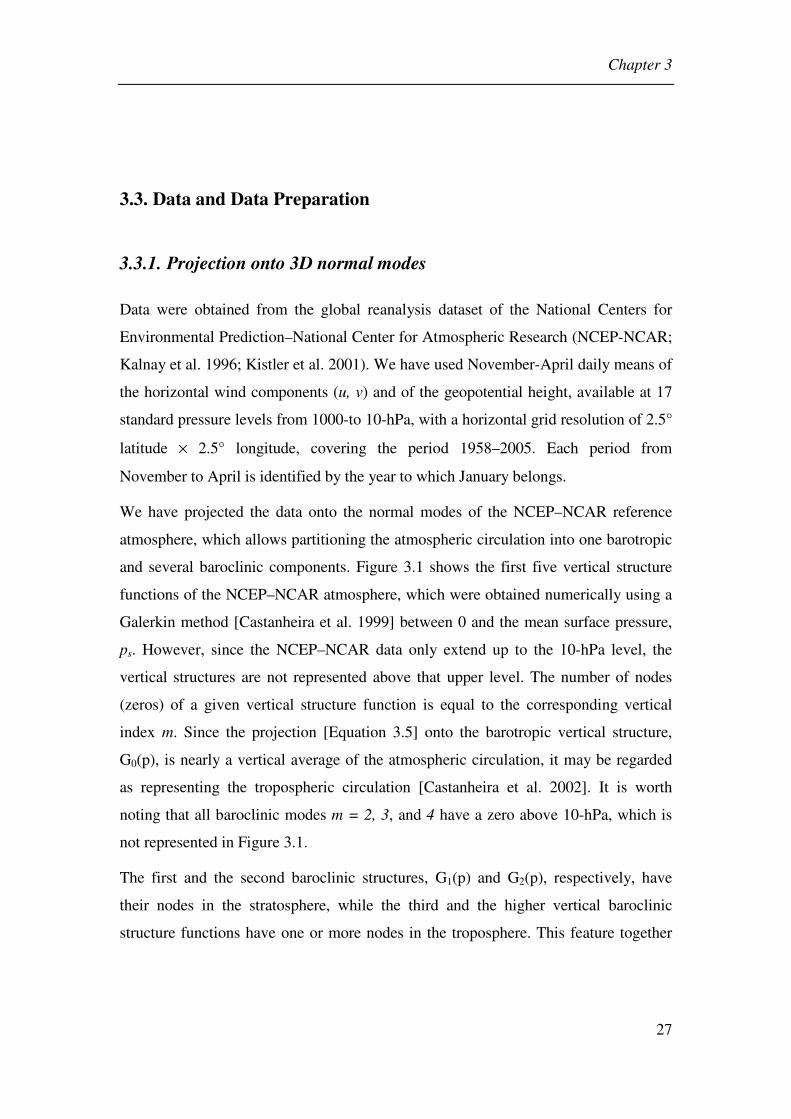
Chapter 3
27
3.3. Data and Data Preparation
3.3.1. Projection onto 3D normal modes
Data were obtained from the global reanalysis dataset of the National Centers for
Environmental Prediction–National Center for Atmospheric Research (NCEP-NCAR;
Kalnay et al. 1996; Kistler et al. 2001). We have used November-April daily means of
the horizontal wind components (u, v) and of the geopotential height, available at 17
standard pressure levels from 1000-to 10-hPa, with a horizontal grid resolution of 2.5°
latitude × 2.5° longitude, covering the period 1958–2005. Each period from
November to April is identified by the year to which January belongs.
We have projected the data onto the normal modes of the NCEP–NCAR reference
atmosphere, which allows partitioning the atmospheric circulation into one barotropic
and several baroclinic components. Figure 3.1 shows the first five vertical structure
functions of the NCEP–NCAR atmosphere, which were obtained numerically using a
Galerkin method [Castanheira et al. 1999] between 0 and the mean surface pressure,
ps. However, since the NCEP–NCAR data only extend up to the 10-hPa level, the
vertical structures are not represented above that upper level. The number of nodes
(zeros) of a given vertical structure function is equal to the corresponding vertical
index m. Since the projection [Equation 3.5] onto the barotropic vertical structure,
G0(p), is nearly a vertical average of the atmospheric circulation, it may be regarded
as representing the tropospheric circulation [Castanheira et al. 2002]. It is worth
noting that all baroclinic modes m = 2, 3, and 4 have a zero above 10-hPa, which is
not represented in Figure 3.1.
The first and the second baroclinic structures, G1(p) and G2(p), respectively, have
their nodes in the stratosphere, while the third and the higher vertical baroclinic
structure functions have one or more nodes in the troposphere. This feature together

Chapter 3
28
with the large amplitude presented by G1(p) and G2(p) in the stratosphere make these
vertical structure functions especially sensitive to the stratospheric circulation
features.
Projections onto the vertical structure functions were then followed by projections
onto the horizontal normal modes [Equation 3.6], allowing to obtain the complex
wave amplitudes, i.e., the coefficients mslwα . Finally the total energy associated with
each planetary Rossby or gravity wave characterized by a given vertical structure m
and a given wavenumber s was obtained by summing the energy as given in Equation
3.7 for all meridional indices l.
Figure 3.1 – Vertical structure functions of the barotropic m = 0 and the first four baroclinic modes (m = 1,…,4) of the NCEP–NCAR atmosphere. It is worth noting that the NCEP–NCAR database only extends up to the 10-hPa level.

Chapter 3
29
3.3.2. PCA
We have also used the 1000- and 500-hPa geopotential height fields and the zonal
wind data as obtained from the European Centre for Medium-Range Weather
Forecasts (ECMWF) ReAnalysis (ERA-40) datasets [Uppala et al. 2005]. We have
computed daily means, with a 2.5° latitude × 2.5° longitude horizontal grid resolution,
for 45 winters (November to March) from 1958 to 2002. A PCA was then performed
on the NH extratropical circulation north of 30ºN at 1000- and 500-hPa isobaric
levels. Vertical connection between the obtained patterns and the vortex strength was
finally assessed by means of lagged correlations between the respective PCs and the
U50 (65) index described bellow.
3.3.3. Stratospheric Polar Vortex Strength Indices
In our study the strength of the polar vortex is represented by means of the
stratospheric Northern Hemisphere annular mode (NAM) time series as computed by
Baldwin and Dunkerton [2001] (NAM indices, covering the period 1958-2006, were
kindly made available by M. Baldwin).
The strength of the stratospheric polar vortex is also represented by the 50-hPa zonal
mean zonal wind at 65ºN, here denoted as the U50 (65) index. Considering the 15-day
running means, the correlation between the NAM index at 50-hPa and the U50 (65)
index is 0.96. Hence, the much simpler zonal mean wind is nearly identical with the
50-hPa NAM index.
3.3.4. Midwinter Sudden Warming Events
Following the World Meteorological Organization (WMO) definition, a major
midwinter stratospheric warming event occurs when the zonal mean zonal wind at
60°N and 10-hPa becomes easterly, and the gradient of 10-hPa zonal mean
Chapter 3
30
temperature becomes positive between 60° and 90°N. Charlton and Polvani [2007]
adhered to this more widely used WMO definition of SSW events (easterly winds at
10-hPa and 60°N) and examined both the NCEP–NCAR and the 40-yr ECMWF
ReAnalysis (ERA-40) datasets in the extended winter (November–March). These
authors developed a more sophisticated algorithm, based on the sign of the zonal
mean zonal wind, to automatically extract SSW events from large datasets and
distinguish between different types of SSW events.
Charlton and Polvani [2007] distinguish between different types of SSW events,
based on the synoptic structure in the middle stratosphere. Following O’Neill [2003],
one type of SSW events, the so-called vortex displacement, is characterized by a clear
shift of the polar vortex off the pole, and its subsequent distortion into a “comma
shape” during the extrusion of a vortex filament; an example is given in Figure 3.2a.
The other type of SSW events, the so-called vortex split, is easily recognizable in that
the polar vortex breaks up into two pieces of comparable size (Figure 3.2b). While
these two types of SSW events are often associated with large amplitudes of
longitudinal wavenumbers 1 and 2, respectively, a simple Fourier decomposition is
not sufficient to identify them [Waugh 1997, their appendix].

Chapter 3
31
Figure 3.2 – Polar stereographic plot of geopotential height (contours) on the 10-hPa pressure surface. Contour interval is 0.4 km, and shading shows potential vorticity greater than 4.0××××10-6 K kg-1 m2 s-1. (a) A vortex displacement type warming that occurred in February 1984. (b) A vortex splitting type warming that occurred in February 1979 (Figure 1 from Charlton and Polvani [2007]).
Table 3.1 shows the list of SSW events that were used in the present work as
identified in the NCEP–NCAR reanalysis dataset by means of the algorithm
developed by Charlton and Polvani [2007]. Since we have restricted the computation
of daily energies to the periods from 1 November to 30 April, and due to the fact that
we will have to compute composites starting 35 days before and ending 35 days after
the central date of each SSW event, we have excluded from the analysis all events
with central dates before 6 December (i.e., one vortex split and two vortex

Chapter 3
32
displacements). However, composites computed for shorter time intervals and
including the three excluded SSW events led to results identical to the ones that will
be presented.
Table 3.1 – List of SSW events that were considered in this work. SSW events were identified in the NCEP–NCAR dataset based on the algorithm developed by Charlton and Polvani [2007]. Letters D and S in the second column identify displacement- and split-type SSW events, respectively. Here ∆T refers to area-weighted means of the polar cap temperature anomaly at the 10-hPa level, during periods from 5 days before up to 5 days after the central dates of each event.
Central date Type ∆∆∆∆T (K) Central date Type ∆∆∆∆T (K)
30 Jan 1958 S 7.8 29 Feb 1980 D 11.5
16 Jan 1960 D 5.9 24 Feb 1984 D 11.1
23 Mar 1965 S 4.4 2 Jan 1985 S 13.0
8 Dec 1965 D 6.7 23 Jan 1987 D 10.2
24 Feb 1966 S 3.1 8 Dec 1987 S 14.1
8 Jan 1968 S 12.0 14 Mar 1988 D 11.7
13 Mar 1969 D 4.3 22 Feb 1989 S 12.8
2 Jan 1970 D 6.8 15 Dec 1998 D 12.7
17 Jan 1971 S 9.6 25 Feb 1999 S 11.0
20 Mar 1971 D -2.9 20 Mar 2000 D 5.3
2 Feb 1973 S 6.6 11 Feb 2001 D 6.3
22 Feb 1979 S 3.7 2 Jan 2002 D 12.9

Chapter 3
33
3.3.5. Stratospheric Final Warming Events
Concurrently, Black et al. [2006] studied the evolution of SFW events. In the
stratosphere each winter season concludes with a rather abrupt transition from
circumpolar westerly winds to easterlies. This annual breakdown of the polar vortex is
known as the stratospheric final warming (SFW). Their observational study on the
relationship between SFW events and the Northern extratropical circulation found that
SFW events strongly organize the large-scale circulation of the stratosphere and
troposphere. SFW events were defined as the final time during which the zonal mean
zonal wind at 70°N drops below 0 without returning to a specified positive threshold
value until the subsequent autumn. The criterion was applied to 5-day averages at 10-
and 50-hPa zonal mean zonal winds with thresholds of 10 and 5 m s-1, respectively.
We will compute composites of daily energies from 40 days before to 20 days after
the central dates of each SFW event identified at the 50-hPa level. Event dates were
kindly made available by R. X. Black and are based on the NCEP–NCAR reanalysis
dataset covering the 47-yr period 1958–2004. The list of SFW events includes the 22
earliest events and the 22 latest events but our composite analysis will restrict to 19
earliest events (i.e. those events with central dates earlier than 20 days before 30
April). If central dates were chosen up to 10 days before 30 April and composites
were built up from 40 days before to 10 days after the central dates of each SFW
event, then a set of 30 events would be retained. However, we have verified that
similar features were obtained with both samples during the common period (i.e. from
40 days before to 10 days after the central dates).

Chapter 3
34
3.3.6. Climatology and Anomalies
For every variable, we have removed the respective seasonal cycle, which was
estimated by computing at each day the respective interannual mean and then by
smoothing the obtained time series of daily interannual means with a 31-day running
average. Daily values of the energy for the total circulation (i.e. climatology +
anomaly field) were computed before the seasonal cycle was removed. Similarly,
daily anomalies of the other fields were obtained by subtracting the seasonal cycle
from the original daily means. A 15-day running mean was applied to the anomalies,
in order to filter out shorter time scales.
On the other hand since we intend to analyze composites of the daily energy during
stratospheric events, there is the need to remove the interannual components, which
for each extended winter was estimated by the respective winter average. Accordingly
all anomalies used in our work represent intraseasonal fluctuations (i.e. departures
from the respective winter averages).
3.3.7. Statistical Significance of Anomalies
Statistical significance of anomalies in the energy composites was assessed by means
of resampling tests, also known as rerandomization or Monte-Carlo tests. This
approach to non-parametrical testing is based on the construction of artificial datasets
of the same size as the actual data from a given real dataset, which are obtained by
resampling the observations [e.g. Wilks 2005]. In single-sample situations a very
useful technique is the so-called “bootstrap”, which operates by construction of the
artificial data sets using sampling with replacement from the original data.
Conceptually, the sampling process is equivalent, in this case, to writing each of the n
data values (say, n periods of daily energies of 60 consecutive days) on n separate
slips of paper and putting all of them in a hat. To construct one bootstrap sample, the

Chapter 3
35
slips of paper are drawn one by one from the hat, with replacement, being this process
repeated a large number of times (typically nB=1,000 to 10,000 random periods). A
particular time series of the original dataset may be drawn several times, or not at all,
in a given bootstrap sample.
Bootstrap is used here to estimate confidence intervals around observed values of a
test statistic. This procedure may be applied to any test statistic, since bootstrap
method does not depend on the analytical form of its sampling distribution.
Confidence regions are easily approached using the percentile method, which is a
straightforward procedure. To form a (1–α)% confidence interval, one simply finds
the values of the parameter estimates defining the largest and the smallest 2B
n α× of
the nB random samples. This method was also used on the subsequent studies, varying
the number of elements on the bootstrap estimate.

4. BRIDGING THE ANNULAR MODE AND NORTH
ATLANTIC OSCILLATION PARADIGMS
In this chapter the annular nature of the leading patterns of the NH winter
extratropical circulation variability is revisited, and evidence is presented of the
separation of both components of annular and non-annular variability of the NH
atmospheric circulation. The analysis relies on a PCA of tropospheric geopotential
height fields and lagged correlations with the stratospheric polar vortex strength and
with a proxy of midlatitude tropospheric zonal mean zonal momentum anomalies.
Results suggest that two processes, occurring at different times, contribute to the
NAM spatial structure. Polar vortex anomalies appear to be associated to midlatitude
tropospheric zonal mean zonal wind anomalies occurring before stratospheric
anomalies. Following polar vortex anomalies, zonal mean zonal wind anomalies of
the same sign are observed in the troposphere at high latitudes. The separation
timescale between the two signals is about 2 weeks. It is suggested that the leading
tropospheric variability patterns found in the literature represent variability associated
with both processes. The tropospheric variability patterns which appear to respond to
the polar vortex variability have a hemispheric scale but show a dipolar structure only
over the Atlantic basin. The dipole resembles the NAO pattern, but with the node line
shifted northward. These results have been published in Castanheira et al. [2007].
The annular versus non-annular variability of the northern winter extratropical
circulation is reassessed on the second part of this chapter, based on reanalysis data
which were dynamically filtered by 3D normal modes. Results show that one half of
the monthly variability of the barotropic zonally symmetric circulation of the NH is
statistically distinct from the remaining variability, and being explained by its leading
EOF alone. The daily time series of the circulation anomalies projected onto the
leading EOF is highly correlated (r ≥ 0.7) to the lower stratosphere NAM indices,
Chapter 4
38
showing that annular variability extends from the stratosphere deep into the
troposphere.
A PCA of the residual variability of the 500-hPa geopotential height field (defined as
the departures from the 500-hPa geopotential height regressed onto the lower
stratosphere NAM index), also reveals a pattern with a zonally symmetric component
at midlatitudes. However, this zonally symmetric component appears as the second
EOF of the residual variability and is the imprint of two independent dipoles over the
Pacific and Atlantic oceans.
These results, accepted for publication in Castanheira et al. [2008], show that a
zonally symmetric component of the middle and lower tropospheric circulation
variability exists at high latitudes. At the middle latitudes, obtained results suggest
that the zonally symmetric component, that has been identified in other works, is
artificially overemphasized by the usage of PCA on single isobaric tropospheric
levels.
4.1. Extratropical Atmospheric Circulation Variability
In this section a review of the state of the art of the extratropical winter variability is
performed following the paper by Wallace and Gutzler [1981]. Section 4.1.1 describes
wintertime extratropical variability of the horizontal circulation in the troposphere and
stratosphere, and vertical coupling is described in the following section. The
discussion and relation between NAO and NAM paradigms is reviewed in Section
4.1.3 and finally the timescale of teleconnection patterns is discussed in section 4.1.4.
4.1.1. Space-time variability of horizontal circulation
Sir Gilbert Walker pioneered early attempts to understand and identify low-frequency
circulation modes. He was the first to use statistical regression methods to search for
significant teleconnection patterns (though he did not actually use the term

Chapter 4
39
‘teleconnections’). He introduced the use of correlation to study teleconnections and
the use of multiple regression to deal with the problem of long-range forecasting. His
pioneering work culminated in the landmark paper of Walker and Bliss [1932], where
three dominant teleconnection patterns were identified: the Southern Oscillation (SO),
the North Atlantic Oscillation (NAO), and the North Pacific Oscillation (NPO).
The usefulness of Walker’s empirical methods was widely recognised and a large
number of researchers have applied them to larger and higher quality data sets. Van
Loon and Rogers [1978] and Rogers [1981] confirmed many of Walker’s results
regarding NAO and NPO.
Wallace and Gutzler [1981] were the first to provide a comprehensive and extensive
summary of teleconnection patterns in the monthly averaged sea level pressure (SLP)
and upper-level geopotential height fields during the NH winter season. They used
correlations and PCA, which they applied to a 15-year record of winter-time monthly
averaged 500-hPa geopotential height fields. Wallace and Gutzler [1981] constructed
one-point correlation maps and introduced the concept of teleconnectivity, which
helps summarising one-point correlation maps of individual teleconnection patterns in
just one map. Wallace and Gutzler [1981] defined “teleconnections” as significant
simultaneous correlations between geopotential heights on a given pressure surface at
widely separated points on earth and “teleconnectivity” as the strongest negative
correlation on each one-point correlation map, plotted at the base grid point. They
further proposed the use of “teleconnectivity” to contrast the strength of
teleconnection patterns for different base points.
These authors identified in the existing literature at least four recurrent spatial patterns
indicative of standing oscillations in planetary waves (i.e. standing wave structures
with geographically distinct and fixed nodes and antinodes) during NH winter, with
timescales on the order of months or longer. These four patterns are the following:
NAO and NPO, both identified by Walker and Bliss [1932], a zonally symmetric
seesaw between sea level pressures in polar and temperate latitudes, first noted by
Chapter 4
40
Lorenz [1951], and the Pacific/North American (PNA) pattern, as labelled by Wallace
and Gutzler [1981].
4.1.1.1. NH winter season teleconnection patterns
Both the NAO and the PNA patterns are strongly evident in Wallace and Gutzler’s
[1981] study and were considered by these authors as teleconnection patterns at
middle and high latitudes of the NH winter season. Wallace and Gutzler [1981]
described NAO as being associated with fluctuations in the strength of the
climatological mean jet stream over the western Atlantic. The PNA pattern included
in turn a north-south seesaw in the central Pacific somewhat reminiscent of the NPO
as mentioned by Walker and Bliss [1932] and Bjerknes [1969], together with centres
of action over western Canada and the south-eastern United States.
Figure 4.1 shows the teleconnectivity maps for SLP and 500-hPa geopotential height.
Figure 4.1a confirms the SLP patterns associated with the NAO and NPO as described
by Walker and Bliss [1932]. The dipole shaped pattern in the eastern North Pacific
may be considered as a reflection of another major teleconnection, the PNA.
In addition to these two main teleconnection patterns, both characterized by north-
south seesaws or standing oscillations in the sea level pressure field with a node
located near 50ºN latitude, Wallace and Gutzler [1981] stated that the leading
eigenvector of the correlation matrix of the sea level pressure field is dominated by a
planetary scale, zonally symmetric seesaw between sea level pressures in the polar
cap region and lower latitudes. These authors noted also that a similar pattern of
pressure anomalies has been observed in connection with two stratospheric
phenomena, sudden warmings and the quasi-biennial oscillation (QBO).
Whilst the sea level pressure statistics presented by Wallace and Gutzler [1981] were
dominated by negative correlations between the polar region and temperate latitudes,
most of them with only one or two well-defined centres of action at the earth’s
surface, the 500-hPa statistics were dominated by patterns of a more regional scale,
which display a nearly equivalent barotropic structure with amplitudes increasing with

Chapter 4
41
height. According to these authors, their structure at these levels resembles that of
forced stationary waves on a sphere, because at mid-tropospheric levels they are
wavelike in appearance and characterized by multiple centres of action. That is, the
horizontal scale and spatial orientation of the patterns resemble the steady, linear
response of a spherical atmosphere to thermal and/or orographic forcing [Hoskins and
Karoly, 1981].
Figure 4.1 – Strongest negative correlation i
ρ on each one-point correlation
map, plotted at the base grid point (originally referred to as “teleconnectivity”) for (a) SLP and (b) 500-hPa height. Correlation fields were computed over 45 winter months from 1962-1963 to 1976-1977. Negative signs have been omitted and correlation coefficients multiplied by 100. Regions where 60
iρ < are
unshaded; 60 75i
ρ≤ < stippled lightly; 75i
ρ≤ stippled heavily. Arrows
connect centres of strongest teleconnectivity with the grid point, which exhibits strongest negative correlation on their respective one-point correlation maps (Figure 7 from Wallace and Gutzler [1981]).

Chapter 4
42
Another important result stressed by Wallace and Gutzler [1981] is that there are
some notable differences between their eigenvector patterns and their teleconnection
patterns. According to these authors, the latter tend in general to be somewhat more
localized, with fewer strong centres of action, explaining a larger fraction of the local
variance of 500-hPa height in the vicinity of those centres of action. So, the main
advantages of the teleconnection patterns are their somewhat more localized spatial
structure which facilitates their dynamical interpretation, their greater efficiency at
explaining the local variance of the 500-hPa height field, and the simplicity with
which their pattern indices can be computed.
Wallace and Gutzler’s [1981] review study was followed by a large number of studies
of low-frequency atmospheric variability (i.e. variability of the planetary waves on
time scales of several weeks upward to several years), which have produced a diverse
and occasionally confusing set of teleconnection patterns, dynamical modes and
oscillations [Barnston and Livezey 1987; Trenberth and Hurrell 1994; Wallace et al.
1995; Mantua et al. 1997; Thompson and Wallace 1998; 2000; Honda and Nakamura
2001]. Barnston and Livezey [1987] list in their Appendix B some of the patterns of
variability identified prior to that time, and they present similar winter results based
on a high resolution 35-year period of record. These authors have identified some less
obvious patterns and provide further details on the better-known ones. Barnston and
Livezey [1987] stress that the NAO is the only pattern found for every month of the
year, which systematically contracts northward in summer and expands southward in
winter, being both the strongest winter and the strongest summer patterns (Figures 4.2
and 4.3). Using twice-daily data these authors replicated their own results using
monthly, 3-month and 10-day means of 700-hPa height, stressing in their work that
results using 10-day means point the way to use a larger sample without noticeably
obscuring the low-frequency signal.
It may be noted that the patterns that have emerged in all these studies have been
conditioned not only by the different analysis techniques used but also by the spatial
domain of the analysis, the way in which seasonality is treated, and the time interval
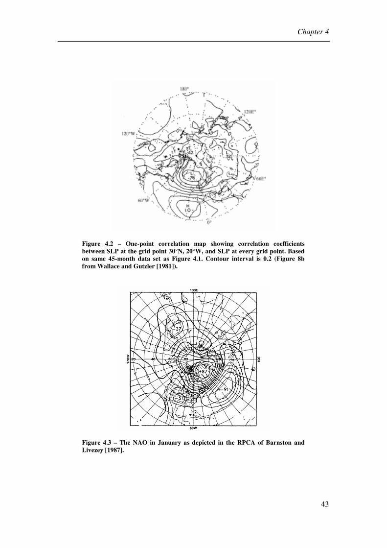
Chapter 4
43
Figure 4.2 – One-point correlation map showing correlation coefficients between SLP at the grid point 30°N, 20°W, and SLP at every grid point. Based on same 45-month data set as Figure 4.1. Contour interval is 0.2 (Figure 8b from Wallace and Gutzler [1981]).
Figure 4.3 – The NAO in January as depicted in the RPCA of Barnston and Livezey [1987].
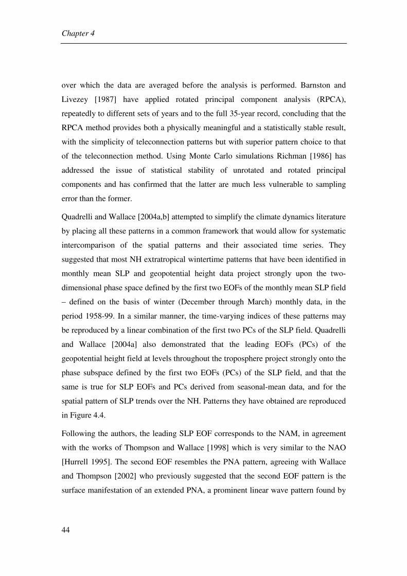
Chapter 4
44
over which the data are averaged before the analysis is performed. Barnston and
Livezey [1987] have applied rotated principal component analysis (RPCA),
repeatedly to different sets of years and to the full 35-year record, concluding that the
RPCA method provides both a physically meaningful and a statistically stable result,
with the simplicity of teleconnection patterns but with superior pattern choice to that
of the teleconnection method. Using Monte Carlo simulations Richman [1986] has
addressed the issue of statistical stability of unrotated and rotated principal
components and has confirmed that the latter are much less vulnerable to sampling
error than the former.
Quadrelli and Wallace [2004a,b] attempted to simplify the climate dynamics literature
by placing all these patterns in a common framework that would allow for systematic
intercomparison of the spatial patterns and their associated time series. They
suggested that most NH extratropical wintertime patterns that have been identified in
monthly mean SLP and geopotential height data project strongly upon the two-
dimensional phase space defined by the first two EOFs of the monthly mean SLP field
– defined on the basis of winter (December through March) monthly data, in the
period 1958-99. In a similar manner, the time-varying indices of these patterns may
be reproduced by a linear combination of the first two PCs of the SLP field. Quadrelli
and Wallace [2004a] also demonstrated that the leading EOFs (PCs) of the
geopotential height field at levels throughout the troposphere project strongly onto the
phase subspace defined by the first two EOFs (PCs) of the SLP field, and that the
same is true for SLP EOFs and PCs derived from seasonal-mean data, and for the
spatial pattern of SLP trends over the NH. Patterns they have obtained are reproduced
in Figure 4.4.
Following the authors, the leading SLP EOF corresponds to the NAM, in agreement
with the works of Thompson and Wallace [1998] which is very similar to the NAO
[Hurrell 1995]. The second EOF resembles the PNA pattern, agreeing with Wallace
and Thompson [2002] who previously suggested that the second EOF pattern is the
surface manifestation of an extended PNA, a prominent linear wave pattern found by
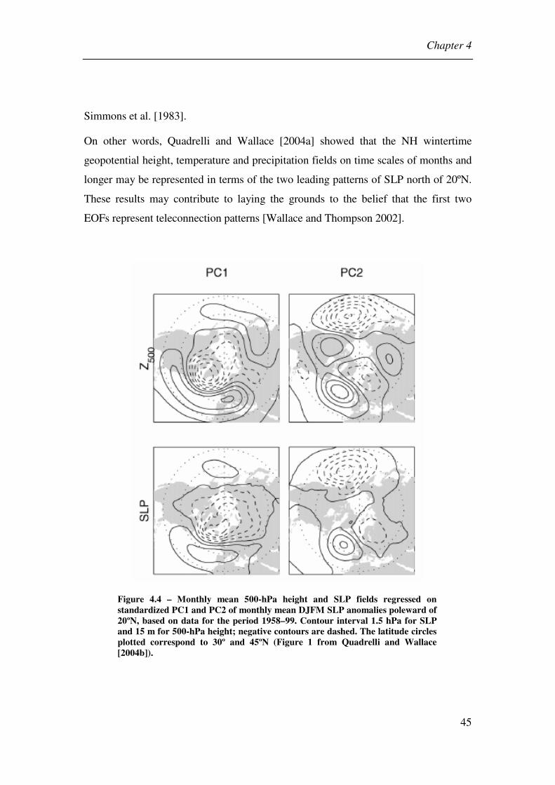
Chapter 4
45
Simmons et al. [1983].
On other words, Quadrelli and Wallace [2004a] showed that the NH wintertime
geopotential height, temperature and precipitation fields on time scales of months and
longer may be represented in terms of the two leading patterns of SLP north of 20ºN.
These results may contribute to laying the grounds to the belief that the first two
EOFs represent teleconnection patterns [Wallace and Thompson 2002].
Figure 4.4 – Monthly mean 500-hPa height and SLP fields regressed on standardized PC1 and PC2 of monthly mean DJFM SLP anomalies poleward of 20ºN, based on data for the period 1958–99. Contour interval 1.5 hPa for SLP and 15 m for 500-hPa height; negative contours are dashed. The latitude circles plotted correspond to 30º and 45ºN (Figure 1 from Quadrelli and Wallace [2004b]).

Chapter 4
46
4.1.1.2. AO and Annular Modes
The annular modes (AM) are dominant variability patterns that arise in the Northern
and Southern extratropics throughout the troposphere and stratosphere. These AM
describe a meridional seesaw between the polar region and midlatitudes. Most
prominent among these is the Northern AM (NAM) or Arctic Oscillation which has
been introduced by Thompson and Wallace [1998] as the leading EOF of the surface
pressure.
Following the earlier studies of Lorenz [1951] and Kutzbach [1970], Thompson and
Wallace [1998; 2000] and Thompson et al. [2000] have given evidence to the
importance of the pattern of variability they refer to as the Arctic Oscillation (AO).
This pattern, known today indistinctly as AO or NAM, is highly correlated with the
NAO pattern. According to Wallace [2000], although the two patterns are highly
correlated, there is a clear distinction that could play a guiding role in how we attempt
to understand physical mechanisms in the NH variability.
Usually defined as the first EOF of the mean sea level pressure field in the NH, the
AO is a robust result from EOF analysis of that field on timescales from weeks to
decades in any season [Kutzbach 1970; Thompson and Wallace 1998]. This is now a
conventional definition of the ‘‘annular mode’’ [Thompson and Wallace 2000],
although the correspondence of EOFs to the dynamical modes of climate generally
cannot be made precise [North 1984].
On the other hand, Thompson and Wallace [1998] stated that the leading EOF of the
wintertime sea-level pressure field resembles the NAO in many aspects, but its
primary centre of action covers more of the Arctic, giving it a more zonally
symmetric appearance. Coupled to strong fluctuations at the 50-hPa level at the
intraseasonal, interannual, and interdecadal time scales, this “Arctic Oscillation” may
be interpreted as the surface signature of modulations in the strength of the polar
vortex aloft. It is proposed by Thompson and Wallace [1998] that the zonally
asymmetric surface air temperature and mid-tropospheric circulation anomalies
Chapter 4
47
observed in association with the AO may be secondary baroclinic features induced by
land-sea contrasts.
A characteristic of the AM is its vertical extension into the stratosphere and its
downward propagation [Baldwin and Dunkerton, 1999]. This latter issue will be
analised in detail in the next section.
According to Baldwin and Dunkerton [2001], variations in the strength of the polar
vortex are well characterized by “annular modes,” which are hemispheric-scale
patterns characterized by synchronous fluctuations in pressure of one sign over the
polar caps and of opposite sign at lower latitudes. They used daily November to April
data to independently define the annular mode indices at each of 26 pressure levels
from 1000- to 0.316-hPa, during the period 1958-1999. At each pressure level the
annular mode is the first EOF of 90-day low-pass filtered geopotential anomalies
north of 20°N. Daily values of the annular mode, spanning the entire 42-year data
record, were calculated for each pressure level by projecting daily geopotential
anomalies onto the leading EOF patterns.
In this paper the authors stated that, in the stratosphere, annular mode values are a
measure of the strength of the polar vortex, while the near-surface annular mode is
called the “Arctic Oscillation” (AO) [Thompson and Wallace 1998], which is
recognized as the NAO [Hurrell 1995; Wallace 2000] over the Atlantic sector.
According to Baldwin and Dunkerton [2001] their observations suggest that large
circulation anomalies in the lower stratosphere are related to substantial shifts in the
AO/NAO and that these stratospheric signals may be used as a predictive tool. Their
results further suggest the possibility that other changes in the stratosphere (e.g., from
volcanic aerosols, solar irradiance or greenhouse gases) could in turn be related to
surface weather if they affect the likelihood or timing of extreme circulation events in
the polar lower stratosphere.
However, while in the stratosphere the NAM is simply interpreted as representing the
variability of polar vortex strength, the interpretation in the troposphere is much more

Chapter 4
48
difficult due to the entangled sources of tropospheric variability. This will be subject
to further investigation and discussion in this thesis.
Thompson and Wallace [2000] show that the structures of the NH and SH annular
modes are remarkably similar, not only in the zonally averaged geopotential height
and zonal wind fields, but also in the mean meridional circulations. The authors note
that they both exist year-round in the troposphere, though they amplify with height
upward into the stratosphere during those seasons in which the strength of the zonal
flow is conducive to strong planetary wave-mean flow interactions, namely midwinter
in the NH and late spring in the SH, which they defined as “active seasons”.
The Southern Hemisphere (SH) counterpart of the NAM, referred to as Antarctic
Oscillation [Gong and Wang 1999] or Southern Annular Mode (SAM), is a large-
scale pattern of climate variability characterized by fluctuations in the strength of the
SH circumpolar flow. Stratospheric AM is “active” only in certain months,
comprising the boreal winter (January to March) for the NAM and the SH late spring
(November) for the SAM. The stratospheric circulation is most variable during
winter, when the cold, cyclonic polar vortex varies in strength and is disturbed by
planetary-scale Rossby waves. These waves originate mainly in the troposphere and
transport westward angular momentum upward, where they interact with the
stratospheric flow. In particular, the SAM is “inactive” during austral winter
[Thompson and Wallace 2000].
Thompson et al. [2005] examined the temporal evolution of the tropospheric
circulation following large-amplitude variations in the strength of the SH stratospheric
polar vortex in data from 1979 to 2001 as well as following the SH sudden
stratospheric warming of 2002. In both cases, anomalies in the strength of the SH
stratospheric polar vortex precede similarly signed anomalies in the tropospheric
circulation that persist for more than 2 months. These SH tropospheric circulation
anomalies reflect a bias in the polarity of the SAM. Consistent with the climate
impacts of the SAM, variations in the stratospheric polar vortex are also followed by

Chapter 4
49
coherent changes in surface temperatures throughout much of Antarctica.
Results presented in Thompson et al. [2005] are remarkably similar to those observed
in association with anomalies in the NH stratospheric polar vortex, as documented in
Baldwin and Dunkerton [2001]. Thus, results provide independent verification for the
observed relationships between long-lived anomalies in the NH stratosphere and the
surface climate. One notable difference between the two hemispheres is the enhanced
persistence of the SH anomalies. In the NH, major stratospheric events are followed
by anomalies in the lower stratosphere and troposphere that persist for up to circa 60
days; in the SH such events are followed by anomalies in the lowermost stratosphere
and troposphere that persist for up to circa 90 days. The enhanced persistence of
anomalies in the SH stratosphere is consistent with the relative dearth of dynamical
forcing there.
Thompson et al. [2005] results add to a growing body of evidence that suggests that
stratospheric variability plays an important role in driving climate variability at
Earth’s surface on a range of time scales.
4.1.2. Vertical Coupling
There are several techniques that may be used to isolate important coupled modes of
variability between time series of two fields, and several approaches have been
applied to geophysical data. The work of Kutzbach [1967] was decisive in the use of
PCA in climate research by revealing that two or more field variables may be
combined in the same PCA to document the relationships between fields. Bretherton
et al. [1992] reviewed several methods for finding correlated patterns between two
fields.
By comparing methods (CPCA, CCA and SVD) applied to a simple but geophysically
relevant model these authors introduced a conceptual framework for comparing
methods that isolate important coupled modes of variability between time series of
two fields. They compare the quantitative performance of the methods in isolating a

Chapter 4
50
coupled signal as they vary parameters such as the spatial localization of the coupled
signal, the number of sampling times, the number of grid points in each field, and the
ratio of the coupled signal amplitude to uncoupled variability. In a companion paper,
Wallace et al. [1992] have compared the performance of CPCA, CCA and SVD
applied to a geophysical problem, the interannual coupling between wintertime
Pacific SST anomalies and the anomalies in the atmospheric 500-hPa geopotential
height field over the North Pacific, illustrating that SVD clearly isolates the two most
important extratropical modes of variability in the studied case.
In the works of Perlwitz and Graf [1995] and of Thompson and Wallace [1998] the
statistical analysis was repeated for different tropospheric levels allowing studying the
vertical structure of the mode. Thompson and Wallace [1998] refer to growing
evidence indicating that the stratospheric polar vortex is implicated in some of the
interannual variability of climate at the earth's surface. Baldwin et al. [1994], Perlwitz
and Graf [1995], Cheng and Dunkerton [1995] and Kitoh et al. [1996] have
documented the existence of coupling between the strength of the nearly zonally
symmetric polar night jet at the 50-hPa level and a more wavelike pattern reminiscent
of the NAO at the 500-hPa level.
On the other hand, Hurrell [1995] has shown that the NAO modulates wintertime
surface air temperature (SAT) over much of Eurasia: negative SLP anomalies over
Iceland and enhanced westerlies across the North Atlantic at 50ºN (i.e. the positive
polarity of the NAO) are associated with positive SAT anomalies extending from
Great Britain and Scandinavia far into Siberia. Hurrell [1996] went on to demonstrate
that the upward trend in the NAO during the past 30 years accounts for much of the
warming in SAT averaged over the domain poleward of 20ºN. Kodera and Yamazaki
[1994], Graf et al. [1995], and Kodera and Koide [1997] have suggested the
possibility of a dynamical linkage between the recent wintertime warming over
Eurasia and a strengthening of the polar night jet, Robock and Mao [1992], Graf et al.
[1994] and Kodera [1994] have invoked similar linkages to explain the observed
positive SAT anomalies over Eurasia during the winters following major volcanic

Chapter 4
51
eruptions.
Additionally, Thompson and Wallace [1998] stated that their results confirm the
existence of deep vertical coupling in the wintertime polar vortex and its relation to
SAT anomalies over Eurasia and the Northwest Atlantic during an extended
(November-April) winter season. Whereas the studies of Baldwin et al. [1994],
Perlwitz and Graf [1995], Cheng and Dunkerton [1995] and Kitoh et al. [1996] have
represented the tropospheric circulation in terms of the 500- or 850-hPa height fields,
Thompson and Wallace [1998] have emphasized the SLP field. These authors have
shown that fluctuations in the intensity of the stratospheric circulation are linked to
the leading EOF of SLP, a robust, quasi-zonally symmetric mode of variability that
has received much less attention than the more wavelike teleconnection patterns that
dominate the leading EOFs of the mid-tropospheric geopotential height field. This
deep vertical coupling conspicuously prevails through a wide range of frequencies
and is simulated in modelling studies of Kitoh et al. [1996], Kodera et al. [1996] and
Volodin and Galin [1998].
In their work Thompson and Wallace [1998] hypothesize that strong coupling
between troposphere and stratosphere is intrinsic to the dynamics of the zonally
symmetric polar vortex; i.e., that under certain conditions, dynamical processes at
stratospheric levels may affect the strength of the polar vortex all the way down to the
Earth's surface through the combined effects of an induced, thermally indirect mean
meridional circulation analogous to the Ferrell cell and induced changes in the
poleward eddy fluxes of zonal momentum at intermediate levels.
They further speculate that the tropospheric signature of these induced fluctuations
would be zonally symmetric were it not for the existence of land-sea contrasts. A
stronger zonal flow should advect more mild marine air into the interior of the
continents, cold continental air over the western oceans, and increase the frequency of
Atlantic cyclones tracking through the Kara Sea [Rogers and Thompson 1995],
thereby inducing a pattern of SAT anomalies much like that described.

Chapter 4
52
Thompson and Wallace’s [1998] work prompted Baldwin and Dunkerton [2001] to
look higher in the atmosphere for AO connections. They found downward links as
well as upward ones. A switch from a strong stratospheric vortex to a weak one would
move down through the stratosphere, entering the troposphere and reaching the
surface as a weakening and diversion of the AO’s westerly winds. Because it may
take a few weeks for a switch to get from the vortex to the AO, predicting a switch a
week or two ahead looked possible.
Circulation regimes in the stratosphere tend to persist for several weeks or more, but
the stratospheric circulation is generally regarded as having little influence on surface
weather patterns. Baldwin and Dunkerton [2001] have taken a more detailed look at
42 years of vortex and AO wintertime behaviour and found that the connection may
be a persistent one. Once a major switch reaches the lower stratosphere, the vortex
remains unusually weak or strong for an average of 60 days, which should let
forecasters predict extremes in the underlying AO and the accompanying likelihood
of weather extremes out as far as a month or two.
Stratospheric and tropospheric annular mode variations are sometimes independent of
each other, but (on average) strong anomalies just above the tropopause appear to
favor tropospheric anomalies of the same sign. Opposing anomalies are possible, but
anomalies of the same sign dominate the average.
Using daily data (stratospheric weather maps) to identify large stratospheric
circulation anomalies, Baldwin and Dunkerton [2001] then examined time averages
and variability of the near-surface circulation during 60-day periods after the onset of
these anomalies. This methodology makes it clear that large stratospheric anomalies
precede tropospheric mean-flow anomalies and may therefore be useful for
tropospheric weather prediction. From the observed time delay they speculated that
the stratospheric anomalies might also have a causal role in creating the subsequent
tropospheric anomalies. However, in a later work, Polvani and Waugh [2004] showed
that strong (weak) vortex events are preceded by weak (strong) eddy heat anomalies
Chapter 4
53
at 100-hPa. Furthermore, they demonstrated that anomalously strong (weak)
integrated eddy heat flux at 100-hPa are followed by anomalously large (small)
surface values of the AO index up to 60 days following each event.
4.1.3. NAO and NAM paradigms
As a consequence of the referred studies the identity of the NAO has become a
subject of a debate. An alternative teleconnection, termed the AO, also known as
NAM, has been suggested by Thomson and Wallace [2000], who argued that the AO
shows a closer link with Eurasian SAT than the NAO. These authors found that the
AO resembles the NAO but its primary centre covers more of the Arctic. The AO
exhibits a distinct signature in the geopotential height and temperature fields marked
by a zonally symmetric, equivalent barotropic structure. Thompson and Wallace
[1998] also linked the recent climatic trends (warming of the lower troposphere over
Eurasia) with the AO and the strengthening of the westerlies at subpolar latitudes with
weakening of the jet stream at low latitudes.
Today, there is a strong difference in opinions among the meteorological community
on which teleconnection pattern, NAO or AO, deserves more physical meaning.
Ambaum et al. [2001] concluded that NAO is more physically relevant and robust for
NH variability than AO, whereas Wallace [2000] had suggested that NAO and AO
were two paradigms of the same phenomenon, arguing that these could not be equally
valid and proposing some methods of distinguishing between them. On a recent work,
Quadrelli and Wallace [2004a] agree that the proposed coordinate axes (referred
above on section 4.1.1.1) could be alternatively chosen to correspond with NAO and
PNA patterns, as suggested by Ambaum et al. [2001].
Wallace [2000] started a discussion about the importance of the distinction between
NAO and AO. This author argued that the two patterns may represent two different
paradigms of the NH variability, namely the ‘‘regional paradigm’’ (associated with
the NAO) and the ‘‘annular paradigm’’ (associated with the AO). Wallace [2000]

Chapter 4
54
concludes that it is important to come to a consensus as to which of them is more
appropriate.
Consequently Ambaum et al. [2001] examined and compared the definition and
interpretation of the AO with those of the NAO. It is shown by these authors that the
NAO reflects the correlations between the surface pressure variability at its centres of
action, whereas this is not the case for the AO. These authors show that NAO pattern
may be identified in a physically consistent way by applying PCA to various fields in
the Euro-Atlantic region. A similar identification is found in the Pacific region for the
PNA pattern, but these authors claim that no such identification is found for the AO.
Ambaum et al.’s [2001] results suggest that the NAO paradigm may be more
physically relevant and robust for NH variability than is the AO paradigm. However,
they consider that this does not disqualify many of the physical mechanisms
associated with annular modes for explaining the existence of the NAO.
Because of the overlap of the NAO and AO patterns in the Atlantic sector, the time
series of the two patterns are highly correlated. Wallace [2000] notes that the original
definition of the NAO by Walker and Bliss [1932] is more like the modern definition
of the AO than like the currently accepted definitions of the NAO. The NAO points to
a mechanism local to the Atlantic region, whereas the more zonal structure of the AO
led Thompson and Wallace [2000] to suggest that the AO may be a representation of
a fundamentally zonally symmetric mode – an ‘‘annular mode’’ – modified by
zonally asymmetric forcings, such as topography.
According to Ambaum et al. [2001], although the NAO and AO time series are highly
correlated, the differences of the patterns suggest different underlying basic physical
mechanisms. Moreover, these authors also showed that the AO may be an artefact of
EOF analysis. Considering the three mean sea level pressure centres of action in the
AO (Azores 42ºN, 15ºW; Iceland 67ºN, 9ºW; Pacific 44ºN, 168ºW) they showed that
although the coupling between the Atlantic and Pacific regions is weak, as expressed
by their covariances in the covariance matrix for this three-component system, the

Chapter 4
55
dominant EOF for this system has strong loadings in both regions. Ambaum et al.
[2001] argue that the AO is mainly a reflection of similar behaviour in the Pacific and
Atlantic basins, namely, the tendency in both ocean basins for anticorrelation between
geostrophic winds near 35º and 55ºN. These authors further state that the
teleconnections (i.e. covariance structures) in a dataset between the three centres of
action do not match the AO pattern. Through one-point correlation maps for both the
Pacific and Icelandic centres of action in the AO, they suggest that the Pacific centre
of action is related to PNA variability [Wallace and Gutzler 1981, and references
therein], whereas the Atlantic centres are related to NAO variability.
Ambaum et al. [2001] also noted that the lack of correlation between the Pacific and
Atlantic regions had also been observed in the strengths of the zonal jets by Ting et al.
[2000] and by Barnett [1985], who hypothesized that on longer timescales the
signatures of the Southern Oscillation and the NAO may be joined in the first EOF of
sea level pressure.
This issue also had the attention of Deser [2000] who analyzed the teleconnectivity of
the three centres of the surface NAM (the Arctic Oscillation pattern). The author
concluded that the correlation between the Pacific and Azores centres of action is not
significant and that the AO therefore cannot be viewed as reflecting such a
teleconnection. Deser [2000] suggested that the AO reflects independent
teleconnectivity between the variability over each ocean basin and the variability over
the polar cap. These results also support the NAO paradigm as well as Ambaum et
al.’s [2001] conclusions: winter extratropical tropospheric circulation variability is
dominated by a regional meridional seasaw over the Atlantic basin (the NAO) and a
wave train pattern over the Pacific/North American sector (the PNA).
Castanheira and Graf [2003] have also addressed this issue. Their analysis showed
that stratospheric circulation controls the correlation between the North Atlantic and
the North Pacific pressure patterns at least in a statistical sense. A teleconnection
between SLP over the North Pacific and the North Atlantic is found during what they

Chapter 4
56
defined as the strong vortex regime (SVR), but not when the polar vortex is weak
(WVR) or just does not exceed the limit of 20ms-1 at 50-hPa near the polar circle.
Another significant result of their analysis concerns the pattern structure of the NAO.
According to Castanheira and Graf [2003] if the analysis takes into consideration that
a strong and a weak polar vortex represent two different regimes of the atmospheric
circulation, the NAO pattern appears as a strict meridional dipole. This result matches
with the findings of Castanheira et al. [2002] that an NAO-like strictly meridional
dipole over the North Atlantic is an eigensolution of the equations of motion
linearized around a layered atmosphere at rest. However, some differences in the
correlation/regression patterns are observed between the two stratospheric vortex
regimes. The teleconnection over the North Atlantic appears to be stronger during the
SVR and the Azores High extends farther over North Africa.
On Castanheira and Graf’s [2003] results the difference between the mean SLP fields
of the two vortex regimes (Figure 4.5) shows a spatial structure close to that of the
first EOF of SLP when computed over the whole extratropical NH [Thompson and
Wallace 1998], the AO pattern. This pattern was interpreted by Monahan et al.
[2001], as a transitional mode between two hemispheric variability regimes. The
characteristic SW to NE tilt of the isobars over the Euro-Atlantic region, found in
these patterns, is also obtained when the SLP EOF is computed only over the Euro-
Atlantic region in winter [Glowienka-Hense 1990]. The same result may be obtained
from three-dimensional linear studies of the coupled lower stratospheric and
tropospheric circulation variability [Perlwitz and Graf 1995; 2001b; Kodera et al.
1999; Deser 2000; Castanheira et al. 2002]. In all these studies the NAO patterns over
the Euro-Atlantic region are oriented in the same way in winter: SW-NE.

Chapter 4
57
Figure 4.5 – Difference between the mean SLP in the two vortex regimes (SVR-WVR). Contour interval is 0.75 mb. Negative contours are dashed and the zero contour line has been suppressed. The shading indicates where the mean difference is significant at least at the 95% confidence level (Figure 8 from Castanheira and Graf [2003]).
4.1.4. The Timescale of teleconnection patterns
Feldstein [2000] questioned the use of monthly or seasonally averaged data on the
study of the properties of low-frequency anomalies, such as the NAO and PNA
teleconnection patterns [e.g., Wallace and Gutzler 1981; Barnston and Livezey 1987],
arguing that such time averaging could obscure some of the underlying dynamical
processes. This should be the case if the timescale of these anomalies would be much
shorter than two months. According to the investigation of persistent anomalies
performed by Dole [1986], the timescale for a number of low-frequency anomalies

Chapter 4
58
may be much less than one month, where it was found that they decay with an
“integral timescale” [Leith 1973] on the order of 15 days.
Feldstein [2000] identified the anomalies through the application of RPCA to daily
unfiltered 300-hPa geopotential height field and examined the timescale of these low-
frequency anomalies by applying spectral analysis to each PC time series. This author
showed that several of the prominent low-frequency anomalies are well described as a
red noise (or first-order) autoregressive process. Feldstein [2000] showed that, for all
dominant atmospheric low-frequency anomalies, the e -folding timescale has a value
between 6 and 10 days, much less than two months. Thus, the key finding of this
study is that the temporal evolution of the NAO and the PNA patterns may be
interpreted as being a stochastic process, and that all of the above teleconnections are
fundamentally short timescale processes.
Feldstein [2000] pointed out that the shortness of these timescales has important
implications since the calculation of monthly and seasonally averaged anomalies
represents a temporal averaging over many shorter timescale fluctuations. When one
intends to increase the signal-to-noise ratio in the data such time averaging is
beneficial, but such is not the case when the goal is to improve our understanding of
the fundamental dynamics of the excitation, maintenance and decay of teleconnection
patterns.
Furthermore, for those low-frequency anomalies that are well described as a Markov
process, Feldstein [2000] investigated whether the interannual variability of these
anomalies could be interpreted as arising from climate noise [e.g., Leith 1973;
Madden 1976; Dole 1986; Feldstein and Robinson 1994], studying whether the
variance associated with interannual fluctuations of anomalies, such as NAO or PNA,
arises from statistical sampling fluctuations associated with the much shorter 6-10 day
fluctuations of that anomaly, as expected in any Markov process. Feldstein [2000]
concluded, at the 95% confidence level, that although climate noise contributes
toward both NAO and PNA interannual variability, some amount of external forcing,
Chapter 4
59
such as interannual variations in SST [e.g., Horel and Wallace 1981; Mo and Livezey
1986], is also playing a key role.
Some recent studies suggest it may be possible that the AO and NAO are the statistics
of stochastic variability constrained by mass and momentum conservation of fluid
motion, and not dynamical oscillations [e.g., Gerber and Vallis 2005; Wittman et al.
2005]. In such case there is no intrinsic distinction between the AO and NAO besides
the domain on which the analysis is applied. On the other hand, if they are dynamical
oscillations, their distinction must remain on the dynamical mechanisms which
control their variability. This will be subject of our study.
4.2. Principal Component Analysis
As described in section 4.1.3, the annular variability mode extends from the
stratosphere down to the surface [Thompson and Wallace 1998; Baldwin and
Dunkerton 1999]. The suggested mechanism underlying the NAM paradigm is the
eddy-mean flow interaction [e.g., Eichelberger and Holton 2002]. In the stratosphere,
geopotential height anomalies are dominated by a zonal symmetric component and
the downward propagation may be interpreted as zonal mean flow-wave interaction.
This is not the case in the troposphere where the geopotential height anomalies reveal
wavy structures of zonal wavenumbers s = 1 and s = 2. Thompson and Wallace
[1998; 2000] suggested that the zonal symmetry is modified, in the troposphere, due
to the topographic and heating field asymmetries and in response to zonal wind
fluctuations. The variability due to the response to surface forcing is superimposed to
the annular variability.
This study discusses the annular nature of the leading isobaric EOFs of the NH winter
extratropical circulation variability. It will be shown that two processes occurring at
different times may constitute the NAM spatial structure.
Chapter 4
60
4.2.1. Extratropical tropospheric circulation variability
The leading EOFs of the geopotential height daily fields at 1000- and 500-hPa are
very similar to the ones found in the literature, based in monthly time scales and
longer. For the sake of comparison, the first three leading patterns are shown in
Figures 4.6 and 4.7, for the 1000- and 500-hPa, respectively. It may be noted that the
sampling errors of the eigenvalues according to North’s Rule of Thumb [North et al.
1982] (as discussed in chapter 3, section 3.2) were calculated taking into
consideration the time series autocorrelation. Only the first EOF is well separated in
both fields.
As discussed in section 3.2.2, although statistically distinct, the first EOFs are not
necessarily physical modes. It is also worth noting that, for the leading EOF
structures, it makes no difference chosing the spatial domain to be the NH
extratropical circulation north of 30º N, as done here, or including lower latitudes
from 20º N as in the works of Thompson and Wallace [1998; 2000] and others.

Chapter 4
61
Figure 4.6 – Regression patterns (EOFs) of the 1000-hPa geopotential height on standardized PCs of 15-days running mean climatological anomalies, north of 30ºN. EOFs 1, 2 and 3 explain 19.0%, 11.8% and 10.3% of the climatological variability, respectively. Contour interval is 10 gpm, and negative contours are dashed.
Figure 4.7 – As in Figure 4.6 but for 500-hPa geopotential height field. EOFs 1, 2 and 3 explain 15.1%, 11.2% and 9.8% of the total variability, respectively. Contour interval is 15 gpm.

Chapter 4
62
Table 4.1 shows a strong correlation between the same order PCs of the 500-hPa and
1000-hPa geopotential height fields. Significant correlation is also observed between
the first and second PCs and between the second and the third PCs, indicating some
dependence on the represented variabilities. The significance levels were calculated
by means of 10,000 random permutations of the years preserving the serial
autocorrelation, as described in section 3.3.7.
Table 4.1 – Correlations between the first three PCs of the 1000-hPa geopotential height and the first three PCs of the 500-hPa geopotential height (boldface values are above the 99% significance level).
1000-hPa
500-hPa PC1 PC2 PC3
PC1 0.84 -0.41 0.06
PC2 0.44 0.76 0.26
PC3 -0.08 -0.20 0.67
4.2.2. Stratospheric-Tropospheric connection
The statistical connection between the tropospheric variability and the stratospheric
annular variability is assessed by calculating the lagged correlations of the
tropospheric PCs with the 50-hPa zonal mean zonal wind at 65ºN, i.e. the U50 (65)
index. Table 4.2 shows the lagged correlations with maximum absolute value and the
lags of occurrence. Positive lags mean that the stratospheric wind is leading. As
expected from other works [e.g., Baldwin and Dunkerton 2001], the leading PCs of
the tropospheric variability show significant correlations with the stratospheric vortex

Chapter 4
63
strength. The smaller but significant correlation between the stratospheric vortex
strength and the second PC of the 500-hPa geopotential height is also worth being
noted. This shows that the leading PC of the 500-hPa geopotential height (the NAM
index [Baldwin and Dunkerton 2001]) does not represent the full linear connection
between the midtroposphere circulation and the stratospheric vortex strength.
Christiansen [2002] also argued the importance of the second EOF for the statistical
connection with the stratospheric vortex.
Table 4.2 – Lagged correlations between the first three PCs of the 1000-hPa (500-hPa) geopotential height and the 50-hPa zonal mean zonal wind at 65ºN (U50 (65)). Shown are the lagged correlations with maximum absolute values, and the numbers in parentheses indicate the lag in days for their occurrence. Positive lags mean that the stratosphere is leading. Boldface values are above the 99% significance level. The last two rows are similar to the first two rows but considering only U50 (65) anomalies above or below one standard deviation.
PC1 PC2 PC3
1000-hPa 0.53(2) -0.11(30) -0.20(-30)
500-hPa 0.47(-2) 0.28(6) -0.12(-13)
50U σ≥ , 1000-hPa 0.73(1) 0.18(12) 0.24(10)
50U σ≥ , 500-hPa 0.67(-4) 0.51(6) 0.15(-30)
To obtain some insight into the origin of the correlations between the U50 (65) index
and the first two 500-hPa PCs, the annularity of the respective EOF patterns is
analyzed. Figure 4.8 shows the meridional profiles of the zonal mean amplitude of the
two first 500-hPa EOFs patterns. Using the geostrophic balance, the zonal mean zonal
wind anomalies associated with each PC are proportional to the slopes of the
meridional profiles of the zonal mean amplitude of the respective EOF patterns. From
Figure 4.8, it may be concluded that EOF1 is associated with strong zonal mean zonal
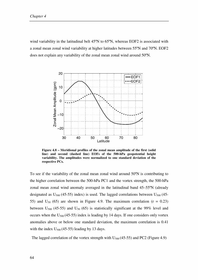
Chapter 4
64
wind variability in the latitudinal belt 45ºN to 65ºN, whereas EOF2 is associated with
a zonal mean zonal wind variability at higher latitudes between 55ºN and 70ºN. EOF2
does not explain any variability of the zonal mean zonal wind around 50ºN.
Figure 4.8 – Meridional profiles of the zonal mean amplitude of the first (solid line) and second (dashed line) EOFs of the 500-hPa geopotential height variability. The amplitudes were normalized to one standard deviation of the respective PCs.
To see if the variability of the zonal mean zonal wind around 50ºN is contributing to
the higher correlation between the 500-hPa PC1 and the vortex strength, the 500-hPa
zonal mean zonal wind anomaly averaged in the latitudinal band 45–55ºN (already
designated as U500 (45-55) index) is used. The lagged correlations between U500 (45-
55) and U50 (65) are shown in Figure 4.9. The maximum correlation (r = 0.23)
between U500 (45-55) and U50 (65) is statistically significant at the 99% level and
occurs when the U500 (45-55) index is leading by 14 days. If one considers only vortex
anomalies above or below one standard deviation, the maximum correlation is 0.41
with the index U500 (45-55) leading by 13 days.
The lagged correlation of the vortex strength with U500 (45-55) and PC2 (Figure 4.9)

Chapter 4
65
Figure 4.9 – Lagged correlations between the 50-hPa zonal mean zonal wind at 65ºN (U50 (65)) and the first two PCs of the 500-hPa geopotential height fields. The curve U500 represents the lagged correlation between the U50 (65) index and the 500-hPa zonal mean zonal wind in the latitudinal belt 45–55ºN. The bottom plot is similar to the top one but considering only U50 (65) anomalies above or below one standard deviation. Positive lags mean that the stratospheric wind is leading.

Chapter 4
66
suggests that there are processes occurring at different times: first, zonal mean wind
anomalies in the midlatitude troposphere lead stratospheric polar vortex anomalies of
the same sign. Once these are established, the positive correlations with PC2 indicate
that stratospheric vortex strength anomalies are leading higher-latitude tropospheric
zonal mean wind anomalies of the same sign by few days. The positive correlations
between U500 (45–55) and U50 (65) are consistent with the lagged cross correlation
between the 300-hPa NAM and the 300-hPa zonally averaged momentum flux
poleward of 20ºN calculated by Baldwin et al. [2003]. As shown by Baldwin et al.
[2003, Figure 4a], the correlations are higher when the upper tropospheric momentum
flux anomalies lead the NAM anomalies. McDaniel and Black [2005, Figure 4c] also
show significant poleward eddy momentum flux anomalies at midlatitude upper
troposphere/lower stratosphere, during the maturing stage of strong positive NAM
events. Hence our interpretation of the correlations in Figure 4.9, which is presented
schematically bellow (Figure 4.10), is that the initial zonal mean momentum
anomalies are shifted to the high latitudes by zonal mean-eddy interactions leading to
vortex anomalies of the same sign. Then the vortex anomalies will progress
downward affecting back the high-latitude troposphere
The correlation between the U50 (65) index and the PC1 is higher and shows a
maximum at a lag shorter than the ones for the maxima of the correlations with the
PC2 and U500 (45-55) index. It may be argued that the fact that the maximum
correlation between the U50 (65) index and the PC1 occurs at negative lags does not
support the idea of a downward influence of the stratospheric vortex variability.
However, this apparent contradiction may be a consequence of the PCA methodology.
The criterion for the identification of the leading EOF/PC is only the maximization of
the explained data variability. The more the variability processes are projected onto
the leading EOF the greater is the explained variability by the leading PC. The blend
of processes may be favoured by the use of 15-days running mean low-pass filtering
of the time series. In fact, the 500-hPa PC1 correlates both with U50 (65) (rmax = 0.47
at lag –2) and with U500 (45-55) (rmax = 0.64 at lag –1) indices, whereas the 500-hPa

Chapter 4
67
PC2 does not show any correlation with U500 (45-55) (rmax = 0.07).
poleward shifting of zonal momentum by eddy-mean flow interactions
zonal mean momentum anomalies in the midlatitude
troposphere (leading by few days)
zonal mean wind anomalies in the high-latitude troposphere (lagged by few days)
stratospheric vortex
anomalies
downward progression of vortex anomalies
Figure 4.10 – Schematic interpretation of the correlations in Figure 4.9.
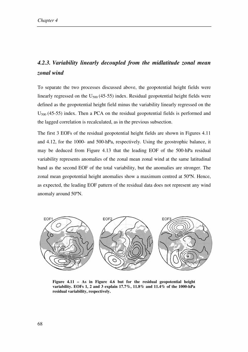
Chapter 4
68
4.2.3. Variability linearly decoupled from the midlatitude zonal mean
zonal wind
To separate the two processes discussed above, the geopotential height fields were
linearly regressed on the U500 (45-55) index. Residual geopotential height fields were
defined as the geopotential height field minus the variability linearly regressed on the
U500 (45-55) index. Then a PCA on the residual geopotential fields is performed and
the lagged correlation is recalculated, as in the previous subsection.
The first 3 EOFs of the residual geopotential height fields are shown in Figures 4.11
and 4.12, for the 1000- and 500-hPa, respectively. Using the geostrophic balance, it
may be deduced from Figure 4.13 that the leading EOF of the 500-hPa residual
variability represents anomalies of the zonal mean zonal wind at the same latitudinal
band as the second EOF of the total variability, but the anomalies are stronger. The
zonal mean geopotential height anomalies show a maximum centred at 50ºN. Hence,
as expected, the leading EOF pattern of the residual data does not represent any wind
anomaly around 50ºN.
Figure 4.11 – As in Figure 4.6 but for the residual geopotential height variability. EOFs 1, 2 and 3 explain 17.7%, 11.8% and 11.4% of the 1000-hPa residual variability, respectively.

Chapter 4
69
Figure 4.12 – As in Figure 4.7 but for the residual geopotential height variability. EOFs 1, 2 and 3 explain 13.5%, 13.1% and 11.6% of the 500-hPa residual variability, respectively.
Figure 4.13 – Meridional profiles of the zonal mean amplitude of the first EOF of the residual 500-hPa geopotential height variability (solid line) and second EOF of the total 500-hPa geopotential height variability (dashed line). The amplitudes are normalized to one standard deviation of the respective PCs.

Chapter 4
70
The leading EOFs of the residual variability at 1000- and 500-hPa (Figures 4.11 and
4.12) show midlatitude centres of opposite sign over the North Atlantic and North
Pacific, whereas the respective leading EOFs of the total variability (Figures 4.6 and
4.7) have two centres of equal polarity, which are taken as an expression of the
annularity. The leading EOFs of the residual variability only show a meridional dipole
over the Atlantic basin resembling the NAO, but with the node line shifted northward.
Table 4.3 shows the correlation between the PCs of the 500- and 1000-hPa residual
geopotential fields. Now, the PCs are paired one to one, and the first two PCs show an
increase in correlation when compared to the values obtained for the total variability
(Table 4.1). It is worth emphasising that the order of the second and third PCs of the
1000-hPa residual geopotential field is switched in Table 4.3. The variances of PC2
and PC3 are very close and their order may have been changed in the process of
computing due to the presence of noise. In fact the EOF patterns associated with PC2
and PC3 of the residual variability (Figure 4.11) are very close to the EOF patterns
associated with PC3 and PC2 of the total variability (Figure 4.6), respectively.
Table 4.3 – As in Table 4.1 but for the residual geopotential height variability (Note that the order of the 1000-hPa PC2 and PC3 was changed in the table).
1000-hPa
500-hPa PC1 PC3 PC2
PC1 0.92 -0.04 0.18
PC2 0.12 0.81 0.02
PC3 -0.15 0.15 0.66
The correlation between the first 3 PCs of the residual variability and the vortex
strength are shown in Table 4.4. Now, only the leading PCs show statistically
significant correlation with the vortex strength and the correlation maxima at both

Chapter 4
71
isobaric levels occur at positive lags and have close values. The curves of lagged
correlations (Figures 4.14 and 4.15) are consistent with a delayed downward influence
of the stratospheric vortex on the residual tropospheric variability.
Nevertheless, when considering the total variability, the maximum of correlation
between the leading PC of 500-hPa geopotential height and the vortex strength occurs
for negative lags, i.e., with the tropospheric variability leading (Figure 4.9). These
results suggest that, after removing the variability linearly dependent on the U500 (45-
55) index, the leading EOFs/PCs of the residual variability mainly capture the
downward influence of the stratospheric vortex variability.
Table 4.4 – As in Table 4.2 but for the residual geopotential height variability.
PC1 PC2 PC3
1000-hPa 0.53(7) 0.16(15) -0.19(8)
500-hPa 0.51(4) -0.17(-20) -0.10(13)
50U σ≥ , 1000-hPa 0.73(7) 0.28(9) -0.23(-10)
50U σ≥ , 500-hPa 0.73(5) -0.24(-25) -0.10(-14)

Chapter 4
72
Figure 4.14 – Lagged correlations between the 50-hPa zonal mean zonal wind at 65ºN and the leading PCs of the total (solid line) and residual (dashed line) variabilities of (top) 1000-hPa and (bottom) 500-hPa geopotential height fields. Positive lags mean that the stratospheric wind is leading.

Chapter 4
73
Figure 4.15 – As in Figure 4.14 but considering only 50-hPa zonal mean zonal wind anomalies above or below one standard deviation.
Chapter 4
74
4.2.3.1. The effect of filtering
Until now, all lagged correlations were based on daily time series smoothed by a 15-
day running mean. It is of interest to assess the effect of the smoothing on the lags.
Lagged correlations as the ones showed in Figure 4.9 were recalculated using
unfiltered (i.e. not averaged) daily time series (Figure 4.16a). Unfiltered time series
for PC1 and PC2 were obtained by projecting the daily unfiltered anomalies onto the
EOF1 and EOF2 of the 500-hPa geopotential height field smoothed by the 15-day
running mean. Figure 4.16a shows the same lag features as those observed in Figure
4.9. The curve representing the lagged correlations between the unfiltered time series
of PC1 and the vortex strength shows a maximum near to zero lag and a shoulder for
negative lags. The maximum and the shoulder suggest, now more clearly, that the
processes underlying the correlation of the U500 (45-55) index and the PC2 with the
vortex strength may be associated with circulation variability which projects also onto
EOF1.
The time separation between the two signals is also clear if one considers only the
intraseasonal variability, i.e., the variability which remains after removing the
seasonal (November to March) means. Figure 4.16b summarizes the main findings of
this study. The lagged correlations between the intraseasonal anomalies of the U50(65)
index and the intraseasonal anomalies of the first two PCs of the 500-hPa total
geopotential height variability are shown together with the U500 (45-55) index, and the
leading PC of the 500-hPa residual geopotential height variability. It may be noted
that only U50 (65) anomalies above or below one standard deviation of the
intraseasonal variability were considered.

Chapter 4
75
Figure 4.16 – As Figure 4.9 (bottom) but (a) considering unfiltered (i.e. not averaged) time series and (b) considering only the intraseasonal variability. The curve PC1res represents the lagged correlation between the U50 (65) index and the leading PC of the 500-hPa geopotential height residual variability.
Chapter 4
76
4.3. Annular versus non-annular circulation variability
Results presented in the previous section suggest that two processes, occurring at
different times, contribute to the NAM spatial structure. It is further suggested that the
leading tropospheric variability patterns found in the literature represent variability
associated with both processes. The tropospheric variability patterns which appear to
respond to the polar vortex variability have a hemispheric scale but show a dipolar
structure only over the Atlantic basin. The dipole resembles the NAO pattern, but
with the node line shifted northward.
In this section an analysis is presented that clearly shows that much of the
tropospheric NAM variability, i.e. the variability projected onto the leading EOF of
geopotential height at single isobaric levels, is not coupled with the variations of the
polar vortex strength. A large fraction of the midlatitude zonal symmetric component
of the tropospheric NAM seems to result from two independent dipolar structures
over the Pacific and the Atlantic oceans. A zonally symmetric component of the
middle and lower tropospheric zonal wind variability seems to only exist at high
latitudes.
4.3.1. 3D normal modes dynamical filtering
As shown by Ambaum et al. [2001] hemispheric EOF analyses of different lower-
tropospheric parameter fields, that one might expect to be dynamically related, may
yield very different results and patterns that are not obviously related. On the other
hand Thompson and Wallace [1998; 2000] and Wallace and Thompson [2002] argue
that a dynamical coupling between the stratosphere and troposphere is manifest in the
annular modes, which characterize deep, zonally symmetric fluctuations of the
geopotential height and zonal wind fields. Having these results in mind it seems
useful to look for the joint variability of the zonal means of geopotential height and
zonal wind at all isobaric levels.
Chapter 4
77
The procedure already described in section 3.2.1 is now applied to the global NCEP-
NCAR reanalysis data (section 3.3.1). Because one is interested in the variability of
the northern extratropical circulation, the southern hemisphere circulation has been
replaced by the specular image of the northern one before the projection onto the
normal modes. Since the extratropical circulation is in very close geostrophic balance,
in the subsequent analysis only symmetric barotropic Rossby modes (i.e., m = 0; α =
2) have been retained in the expansion (Equation 3.4), thus obtaining the 3D normal
mode projection coefficients 2
00lω .
The barotropic 3D normal modes represent a mass weighted vertical mean of the
atmospheric circulation, being therefore very sensitive to the tropospheric circulation.
A PCA on the joint variability of the geopotential and the zonal wind fields requires
that the two fields are adequately weighted. The U and Z components of the zonally
symmetric Rossby modes satisfy the geostrophic balance and the projection onto the
normal modes allows for an appropriate weighting of these two fields. On the other
hand, an EOF analysis on the projection coefficients will retrieve dynamically
consistent patterns for both fields. Hence, the analysis of the joint variability of the
zonal means of the geopotential height and zonal wind at all isobaric levels was
performed by a PCA of the coefficients of the barotropic zonally symmetric Rossby
modes (i.e., m = 0; s = 0; α = 2). Using this procedure, the ageostrophic motions
were filtered away and the geopotential height and wind were simultaneously
weighted in a dynamical self consistent way. The leading EOF (Figure 4.17)
represents one half (50.4%) of the total variability and it is statistically distinct
according to North’s Rule of Thumb [North et al. 1982] (as discussed in chapter 3).
The EOF meridional structures were retrieved by replacing the projection coefficients
2
00lω by the respective EOF loadings (section 3.3.1). The meridional profile of the
zonal mean geopotential height associated with the leading EOF of the 500-hPa
geopotential height field is also represented in the same figure. Before drawing the
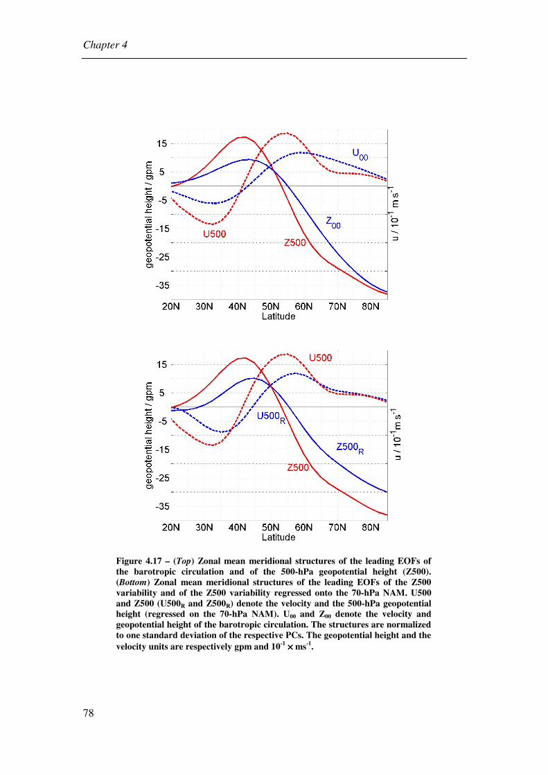
Chapter 4
78
Figure 4.17 – (Top) Zonal mean meridional structures of the leading EOFs of the barotropic circulation and of the 500-hPa geopotential height (Z500). (Bottom) Zonal mean meridional structures of the leading EOFs of the Z500 variability and of the Z500 variability regressed onto the 70-hPa NAM. U500 and Z500 (U500R and Z500R) denote the velocity and the 500-hPa geopotential height (regressed on the 70-hPa NAM). U00 and Z00 denote the velocity and geopotential height of the barotropic circulation. The structures are normalized to one standard deviation of the respective PCs. The geopotential height and the velocity units are respectively gpm and 10-1 ×××× ms-1.

Chapter 4
79
figure, the zonal mean amplitude of the leading EOF of 500-hPa geopotential height
field was divided by the square root of the cosine of the latitude in order to retrieve
the zonal mean meridional profile of the geopotential height. The meridional profile
of the zonal mean zonal wind (U500) associated with the leading EOF of the 500-hPa
geopotential height field was obtained using the geostrophic relationship. The three
first EOF patterns of the 500-hPa geopotential height field are shown in the upper row
of Figure 4.18 for reference purposes. These figures are basically the same as Figure
4.12 except for the fact that the domain is now north of 20ºN and the filtering is 31-
day running means. The results are virtually the same when one uses 15-day running
means instead of 31-day running means, but the leading PCs of the 15-day smoothed
data represent a smaller fraction of the respective variability.
The fact that the leading EOF of the zonally symmetric barotropic Rossby modes
represents annular variability over the whole vertical domain is demonstrated by
Figure 4.19. It shows the lagged correlations between the daily NAM indices and the
projections of daily anomalies onto the first EOF of the barotropic mode. These
projections are highly correlated with the NAM indices over the whole atmosphere,
and a signal of delayed correlation with the high levels in the stratosphere may be
observed. Comparing the zonal mean geopotential height profiles in Figure 4.17 one
observes that the leading EOF of 500-hPa geopotential height field has larger
amplitudes at midlatitudes. At high latitudes it shows amplitudes comparable to those
of the leading EOF of the barotropic zonally symmetric Rossby modes. The
differences of the geopotential height profiles lead to remarkable differences of the
respective zonal mean zonal wind profiles. The leading EOF of 500-hPa geopotential
height field represents a seesaw of zonal mean zonal wind between the subtropics and
midlatitudes, whereas the seesaw is displaced northward in the zonally symmetric
barotropic circulation, presenting stronger zonal wind anomalies at high latitudes.
The leading EOF of the 500-hPa geopotential height field captures much more zonally
symmetric variability in the midlatitudes than the one represented by the leading EOF
of the zonally symmetric barotropic circulation. This suggests that the leading EOF of

Chapter 4
80
the 500-hPa geopotential height field pattern may include variability structures which
are not part of the vertically coherent variations of the annular mode. Clearly the
correlation of the tropospheric NAMs with the barotropic annular mode (Figure 4.19)
is reduced when compared with the stratospheric NAMs. This is especially the case
when the tropospheric NAM leads by more than 5 days.
The lagged correlations in Figure 4.19 are based on unfiltered daily time series and a
signal of delayed correlation is suggested by the asymmetry of correlation curves for
NAM indices at levels above 50-hPa. At stratospheric levels below 50-hPa the
correlation curves are very close and nearly symmetric suggesting a rapid progression
of the circulation anomalies from the lower stratosphere to the troposphere. Then, for
the study of the coupling of the stratospheric and tropospheric circulations, avoiding
the necessity of consideration of lagged effects, it is convenient to use a NAM index
well inside the stratosphere but close to the tropopause. Considering results of Figure
4.19, on the following one chose to represent the polar vortex strength by the 70-hPa
NAM index. However, the results showed to be qualitatively the same if one used the
50-hPa or the 100-hPa NAM indices.
The middle panel in Figure 4.18 shows the regression pattern of the 500-hPa
geopotential height field on the 70-hPa NAM. In order to make the regression and the
EOF patterns comparable, the 500-hPa geopotential height field was also weighted by
the square root of the cosine of the latitude before performing the regression. By
visual inspection one might say that the regression pattern shares the main annular
features of the leading 500-hPa geopotential height field EOF, but with a weaker
Pacific centre. However, comparing the respective meridional structures, shown in the
lower panel of Figure 4.17, it becomes clear that they are different. The regression
pattern shows a zonal mean meridional structure close to the one of the leading EOF
of the barotropic mode (U00 and Z00 in the upper panel of Figure 4.17).

Chapter 4
81
Figure 4.18 – (Top) First three EOF patterns of the 500-hPa geopotential height variability. (Middle) Regression pattern of the Z500 field onto the 70-hPa NAM. (Bottom) As in the top panel, but for the residual variability, i.e. the variability that remained after subtraction of Z500 regressed on the 70-hPa NAM. The patterns are normalized to 1 standard deviation of the respective PCs. The values in the right top of each panel are the percentages of variance represented by each (EOF, PC) pair. Contour interval is 10 gpm, except in the regression pattern where the contour interval is 7.5 gpm.

Chapter 4
82
Figure 4.19 – Lagged correlations between the daily data projections onto the first EOF of the barotropic mode and the NAM indices. Solid curves are for stratospheric NAMs from 10-hPa (black) to 150-hPa (light gray). The dashed red curve is for 1000-hPa NAM and the dashed blue curve is for 500-hPa NAM. Positive lags mean that NAM indices are leading.
From the leading EOF and the regression patterns in Figure 4.18, using the
geostrophic relationship, one may conclude that the largest zonal wind anomalies
must occur in the [90ºW, 30ºE] and the [90ºE, 255ºE] longitude sectors. Figure 4.20
shows the correlations between the zonal means of the 500-hPa zonal winds in each
longitude sector.
The correlations are small and negative at midlatitudes and higher and positive at high
latitudes. The strong negative correlations near the pole are in agreement with the
displacement of the vortex centre over Greenland. This figure shows that positively
correlated zonal wind anomalies corresponding to a true annular component occur
only at high latitudes. The longitude sector over the Pacific, in which the zonal wind
was averaged, is rather broad and its east side is close to the west side of the Atlantic
longitude sector. Considering a larger [90ºE, 255ºE] longitude sector does not
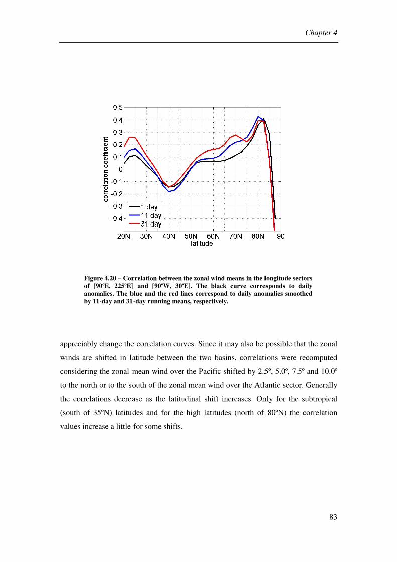
Chapter 4
83
Figure 4.20 – Correlation between the zonal wind means in the longitude sectors of [90ºE, 225ºE] and [90ºW, 30ºE]. The black curve corresponds to daily anomalies. The blue and the red lines correspond to daily anomalies smoothed by 11-day and 31-day running means, respectively.
appreciably change the correlation curves. Since it may also be possible that the zonal
winds are shifted in latitude between the two basins, correlations were recomputed
considering the zonal mean wind over the Pacific shifted by 2.5º, 5.0º, 7.5º and 10.0º
to the north or to the south of the zonal mean wind over the Atlantic sector. Generally
the correlations decrease as the latitudinal shift increases. Only for the subtropical
(south of 35ºN) latitudes and for the high latitudes (north of 80ºN) the correlation
values increase a little for some shifts.
Chapter 4
84
4.3.2. Tropospheric variability decoupled from the stratosphere
By construction both the regression pattern and the leading EOF of the barotropic
mode represent tropospheric annular variability coupled with stratospheric annular
variability. However, it may be possible that there is an annular component of the
tropospheric variability decoupled from the stratosphere. To investigate this
possibility a PCA on the residual 500-hPa geopotential height field that remained after
subtraction of the 500-hPa geopotential height field data regressed linearly onto the
70-hPa NAM was performed following a similar procedure to the one described in
section 4.2.3.
The first 3 EOFs of the residual 500-hPa geopotential height field are shown in the
bottom row of Figure 4.18. Comparing these EOFs with the corresponding EOFs of
the total variability, in the top of the same figure, one observes that the third EOF is
quite insensitive to the stratospheric variability. It is interesting to note that these
patterns are also similar to the third EOF obtained after removing the variability
linearly dependent on the U500 (45-55) index (Figure 4.12), suggesting that this
pattern, which represents a wave train over the Atlantic-European sector, may
represent a true physical mode, since it is insensitive to both the variability linearly
dependent on the U500 (45-55) index and stratospheric variability.
The most pronounced differences are seen in the first two EOFs. The first EOF of the
residual variability shows the PNA structure and a wave train over the Atlantic and
Eurasia like the augmented PNA pattern proposed by Wallace and Thompson [2002].
These results suggest that the first two EOFs of the 500-hPa geopotential height total
variability field represent mixed variability associated with both the PNA and the
stratospheric vortex variability. The second EOF of the 500-hPa geopotential height
residual variability shows two dipoles over the Atlantic and Pacific oceans. As argued
by Gerber and Vallis [2005], performing a PCA on a variability field dominated by
independent dipolar structures, one may end up falsely with leading EOF patterns
Chapter 4
85
with a high degree of zonal symmetry.
Figure 4.21 shows, again, the meridional structures of the first EOF of the total 500-
hPa geopotential height field and the meridional structures of the first two EOFs of
the residual 500-hPa geopotential height field. The meridional structure of the leading
EOF of the residual variability shows a seesaw shifted equatorwards relatively to the
leading EOF of the total variability. On the other hand, the meridional structures of
the first EOF of the total field and of the second EOF of the residual field are very
similar, except at high latitudes, north of 65ºN, where the residual EOF shows a
flattened geopotential profile. The flattening of geopotential at high latitude with a
zonal mean zonal wind close to zero must be due to the absence of the annular
variability regressed on the stratospheric variability.
These results suggest that, at latitudes south of 65ºN the zonal symmetric component
of the first EOF of the total field may largely be the imprint of the two dipolar
structures revealed in the second EOF of the residual variability. Here the question
remains whether the dipolar structures in the second EOF of the residual variability
are independent.
Hence, four anomaly time series of the residual field were defined as follows:
a) Pacific time series (Pac.): the area weighted average of 500-hPa geopotential
height anomaly inside the minimum contour of EOF1 of the residual
variability, over the Pacific.
b) Iceland time series (Ice.): the area weighted average of 500-hPa geopotential
height anomaly inside the minimum contour of EOF2 of the residual
variability, over Iceland and Greenland.
c) Bering Strait time series (Ber.): the area weighted average of 500-hPa
geopotential height anomaly inside the dotted contour on the EOF2 of the
residual variability, over Bering Strait.

Chapter 4
86
Figure 4.21 – (Top) Zonal mean meridional structures of the first EOFs of the total and residual Z500 variabilities. (Bottom) Zonal mean meridional structures of the first EOFs of the total and the second EOF of the residual variability. U500R and Z500R denote the meridional profiles of the velocity and geopotential height associated with the EOFs of the residual variability, respectively.

Chapter 4
87
d) Siberia time series (Sib.): the area weighted average of 500-hPa geopotential
height anomaly inside the maximum contour of EOF3 of the residual
variability, over Siberia.
Figure 4.22 shows the correlation maps between the 500-hPa geopotential height
residual anomalies at each grid point and the four time series defined above.
The correlation with the Pacific time series shows the characteristic PNA pattern. The
secondary wave train over the Atlantic and Eurasia observed in EOF1 of the residual
variability is only reminiscent in the correlation pattern. These results suggest a
regional (not hemispheric) character of the PNA.
The correlation with the Siberia time series shows a pattern similar to both the third
EOFs of the residual and total variabilities, suggesting that both EOFs are capturing
true teleconnectivity. These EOFs show a wave train nearly in quadrature with the
wave train over the Atlantic and Eurasia observed in the EOF1 of the residual
variability. Then it is possible that the PNA, through its Florida centre, may influence
the excitation of the Atlantic/Eurasian wave train represented in the third EOFs
[Reyers et al. 2006]. In such case, the leading EOF of the residual variability would
represent teleconnectivities implied by both the Pacific/North American wave train
and an Atlantic/Eurasian wave train.
The most prominent structures in the correlation maps with the Icelandic and the
Bering Strait time series are two meridional dipolar structures over the respective
ocean basins. The correlations of both time series with grid point anomalies over the
opposite ocean basin is very small, explaining less than 4% of their variabilities. The
correlation map with the Icelandic time series depicts the NAO pattern. It is worth
remarking that similar correlation maps are obtained if one considers the total 500-
hPa geopotential height variability or if 15-day running means are used instead of 31-
day running means.
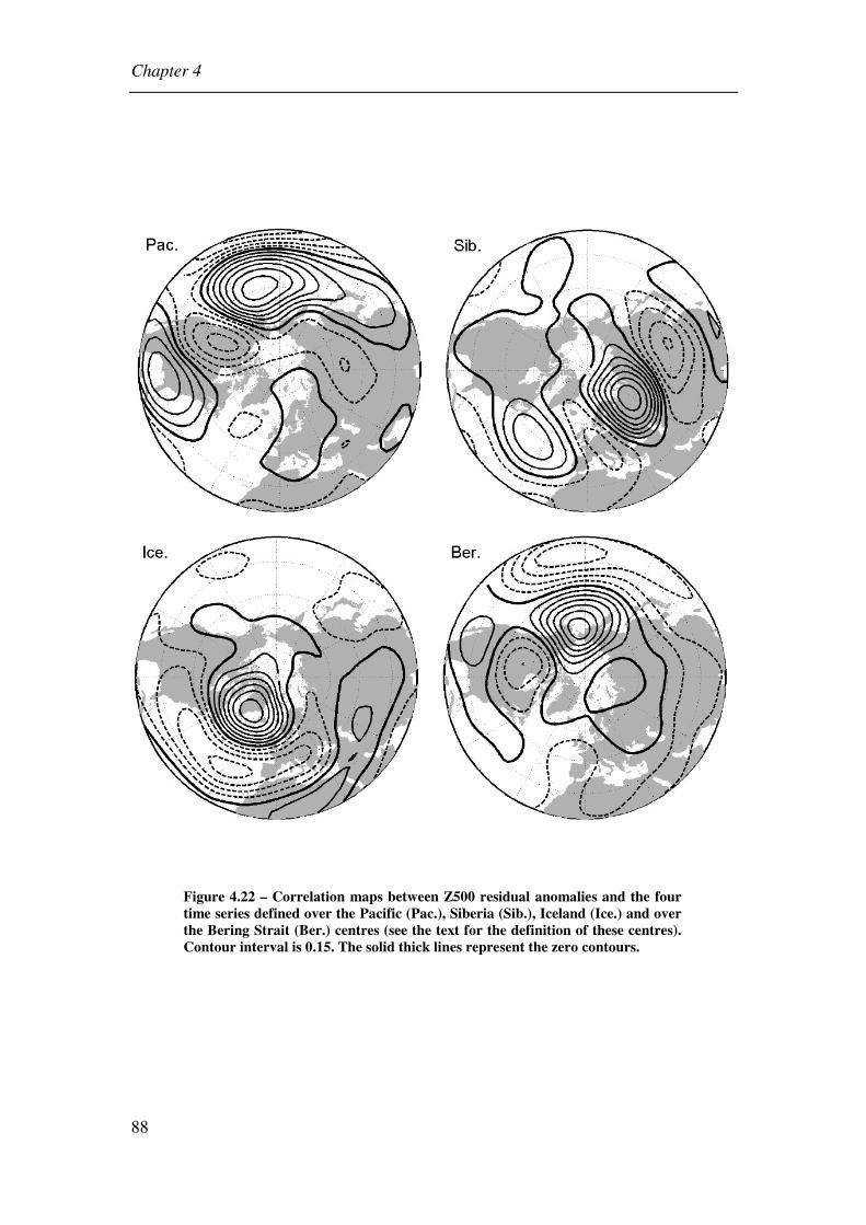
Chapter 4
88
Figure 4.22 – Correlation maps between Z500 residual anomalies and the four time series defined over the Pacific (Pac.), Siberia (Sib.), Iceland (Ice.) and over the Bering Strait (Ber.) centres (see the text for the definition of these centres). Contour interval is 0.15. The solid thick lines represent the zero contours.
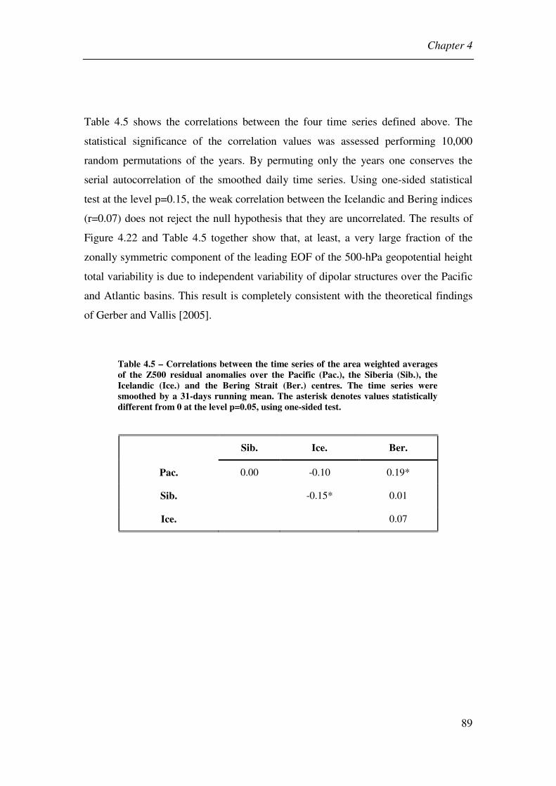
Chapter 4
89
Table 4.5 shows the correlations between the four time series defined above. The
statistical significance of the correlation values was assessed performing 10,000
random permutations of the years. By permuting only the years one conserves the
serial autocorrelation of the smoothed daily time series. Using one-sided statistical
test at the level p=0.15, the weak correlation between the Icelandic and Bering indices
(r=0.07) does not reject the null hypothesis that they are uncorrelated. The results of
Figure 4.22 and Table 4.5 together show that, at least, a very large fraction of the
zonally symmetric component of the leading EOF of the 500-hPa geopotential height
total variability is due to independent variability of dipolar structures over the Pacific
and Atlantic basins. This result is completely consistent with the theoretical findings
of Gerber and Vallis [2005].
Table 4.5 – Correlations between the time series of the area weighted averages of the Z500 residual anomalies over the Pacific (Pac.), the Siberia (Sib.), the Icelandic (Ice.) and the Bering Strait (Ber.) centres. The time series were smoothed by a 31-days running mean. The asterisk denotes values statistically different from 0 at the level p=0.05, using one-sided test.
Sib. Ice. Ber.
Pac. 0.00 -0.10 0.19*
Sib. -0.15* 0.01
Ice. 0.07
Chapter 4
90
4.3.2.1. 1000-hPa geopotential height field
Much of the discussion about the teleconnectivity represented in the NAM/AO
structure in the literature was based on the analysis of the variability of the mean SLP
field and the 1000-hPa geopotential height field (Z1000) [e.g., Thompson and
Wallace 1998; Deser 2000; Ambaum et al. 2001; Wallace and Thompson 2002].
Figure 4.23 shows an analysis similar to the one in Figure 4.18 but for the 1000-hPa
geopotential height field. The regression of the 1000-hPa geopotential height field
anomalies on the 70-hPa NAM reveals a pattern very close to the first EOF of 1000-
hPa geopotential height field (the AO). The spatial correlation between the two
patterns is r = 0.97. The bottom panels of Figure 4.23 show the first three EOFs of the
residual 1000-hPa geopotential height field that remained after regressing out the 70-
hPa NAM. The second and third EOFs seem to be very insensitive to the stratospheric
variability. The first EOF of the residual field is similar to the first EOF of the total
field (their spatial correlation is r = 0.94) but with the relative magnitudes of the
Atlantic and Pacific centres changed. This is because of the regression of 1000-hPa
geopotential height field on the 70-hPa NAM is stronger over the Atlantic area than
over the Pacific.
Since the leading EOFs of the total and residual 1000-hPa geopotential height fields
are similar, one may, again, question if there is a tropospheric annular component
independent from the stratospheric annular variability. To check this possibility in the
1000-hPa geopotential height residual field, the three following time series were
defined:
a) Pacific time series (Pac.): the area weighted average of 1000-hPa geopotential
height anomaly field inside the maximum contour of the EOF1 of the residual
variability, over the Pacific.
b) Iceland time series (Ice.): the area weighted average of 1000-hPa geopotential
height anomaly field inside the minimum contour of EOF1 of the residual
variability, over Iceland and Greenland.

Chapter 4
91
c) Atlantic time series (Atl.): the area weighted average of 1000-hPa geopotential
height anomaly field inside the maximum contour of the EOF1 of the residual
variability, over the Atlantic.
Figure 4.23 – As in Figure 4.18 but for the 1000-hPa geopotential height field (Z1000). Contour interval is 5 gpm.

Chapter 4
92
Figure 4.24 shows the correlation maps between the 1000-hPa geopotential height
residual time series anomalies at each grid point and the three time series defined
above.
Figure 4.24 – Correlation maps between Z1000 residual anomalies and the three 1000-hPa anomaly time series defined over the Atlantic (Atl.), Pacific (Pac.) and Iceland (Ice.) centres (see the text for the definition of these centres). Contour interval is 0.15. The solid thick lines represent the zero contours.
The correlation maps reproduce the NAO dipole and a surface imprint of the PNA
pattern. However, the correlations between the Atlantic centre and the 1000-hPa
geopotential height field anomalies over the Pacific are near zero and even negative
over the northern Pacific. It may be argued, as in Wallace and Thompson [2002], that
the positive correlation between the Atlantic and Pacific centres is “destroyed” by the
anticorrelation associated with the EOF2 pattern. They suggested that the structure of
the EOF2 represents an augmented-PNA teleconnection pattern. By the same
argument they used one must expect that such teleconnection pattern would reinforce
the anticorrelations between the Icelandic centre and the 1000-hPa geopotential height
field anomalies over the Pacific. Nevertheless the anticorrelation between the
Icelandic centre and the 1000-hPa geopotential height field anomalies over the Pacific

Chapter 4
93
Figure 4.25 – (Top) Regression maps of the Z1000 residual anomalies on the three normalized 1000-hPa anomaly time series defined over the Atlantic (Atl.), Pacific (Pac.) and Iceland (Ice.) centres (see the text for the definition of these centres). (Bottom) As in the top but regressing out also the variability associated with the PC2. Contour interval is 5 gpm. The solid thick lines represent the zero contours.
is small and it seems not to be different from the anticorrelation implied by EOF2
itself. In fact, following the procedure of Wallace and Thompson [2002] one obtains
contradicting results. The top row in Figure 4.25 shows the regression maps of the
1000-hPa geopotential height field residual anomalies on the three normalized 1000-
hPa anomaly time series defined above. The regression map on the Atlantic time
series depicts the NAO pattern. On the other hand, the regression map on the
Icelandic time series is similar to the leading EOF. Their spatial correlation is r=-0.83.
The bottom maps in Figure 4.25 also show the same regression maps but after
Chapter 4
94
removing the variability represented by PC2. Now the regression map with the
Atlantic centre shows a centre with equal polarity over the Pacific. However, the
regression on the Icelandic time series lost its centre over the Pacific and depicts the
NAO pattern. Very similar results were obtained when the same analysis is performed
on the total variability instead of the residual variability. Therefore, the above
correlation and regression maps suggest that the Pacific centre of the leading 1000-
hPa geopotential height field EOF does not belong to the teleconnection pattern
represented by the NAO dipole.
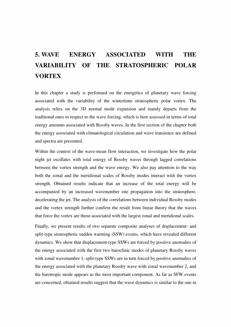
5. WAVE ENERGY ASSOCIATED WITH THE
VARIABILITY OF THE STRATOSPHERIC POLAR
VORTEX
In this chapter a study is performed on the energetics of planetary wave forcing
associated with the variability of the wintertime stratospheric polar vortex. The
analysis relies on the 3D normal mode expansion and mainly departs from the
traditional ones in respect to the wave forcing, which is here assessed in terms of total
energy amounts associated with Rossby waves. In the first section of the chapter both
the energy associated with climatological circulation and wave transience are defined
and spectra are presented.
Within the context of the wave-mean flow interaction, we investigate how the polar
night jet oscillates with total energy of Rossby waves through lagged correlations
between the vortex strength and the wave energy. We also pay attention to the way
both the zonal and the meridional scales of Rossby modes interact with the vortex
strength. Obtained results indicate that an increase of the total energy will be
accompanied by an increased wavenumber one propagation into the stratosphere,
decelerating the jet. The analysis of the correlations between individual Rossby modes
and the vortex strength further confirm the result from linear theory that the waves
that force the vortex are those associated with the largest zonal and meridional scales.
Finally, we present results of two separate composite analyses of displacement- and
split-type stratospheric sudden warming (SSW) events, which have revealed different
dynamics. We show that displacement-type SSWs are forced by positive anomalies of
the energy associated with the first two baroclinic modes of planetary Rossby waves
with zonal wavenumber 1; split-type SSWs are in turn forced by positive anomalies of
the energy associated with the planetary Rossby wave with zonal wavenumber 2, and
the barotropic mode appears as the most important component. As far as SFW events
are concerned, obtained results suggest that the wave dynamics is similar to the one in

Chapter 5
96
displacement-type SSW events. Results presented in this chapter have been published
in Liberato et al. [2007].
5.1. Energy spectra associated with climatological circulation and
wave transience
Although comprehensive studies of normal mode energy spectra may be found in the
literature [e.g., Tanaka and Ji 1995 and references therein], we present in this section,
for reference purposes, the meridional mean energy spectra for the Rossby modes of
wavenumbers s = 1 and 2 associated with the first five vertical structures m.
The spectral characteristics of the synoptic to planetary waves are described by
Tanaka [1985] and Tanaka and Kung [1988] by means of the 3D normal mode
decomposition, including the vertical spectrum. The scheme is referred to as normal
mode energetics. According to the results of their normal mode energetics analysis,
the energy spectrum of the barotropic component of the atmosphere obeys to a
characteristic slope of 2 to 3 power of the eigenfrequency of Laplace’s tidal equation
σ. Tanaka and Kasahara [1992] also found that the energy spectrum is uniquely
determined as a function of the phase speed of the Rossby mode c. Tanaka et al.
[2004] have also shown that the barotropic energy spectrum, E, of the general
circulation may be represented as 2E mc= , i.e., the energy spectrum is proportional to
the squared phase speed of Rossby modes in the general circulation of the atmosphere
(the proportional constant m describes a factored total mass of the atmosphere per unit
area).
Here the analysis of circulation variability was performed by computing the variance
of each coefficient msl
wα , since it is proportional to the transient total energy. It may be
noted that by transient total energy associated with the respective mode we mean the
total energy associated with the deviation of the daily circulation field from the
climatological mean. Assessing the amount of transient energy is a very effective way

Chapter 5
97
of achieving a physically based filtering of the data.
5.1.1. Energy associated with wave transience
Let ( )jwmsl ,τα denote the complex wave amplitudes at day τ of year j. Decomposing
the wave amplitudes in their climatological and anomaly parts and using Equation 3.7,
we may compute the contributions to the climatological (mean) energy associated
with the climatological circulation and the wave transience,
( ) ( ) ( )( )2 2;, , ,s m
msl msl msl
s
p hE w w
c
α α ατ τ τ⋅ = ⋅ + ⋅ (5.1)
where ( )⋅,τx represents the mean over all years for a given day τ , with the
summation index replaced by a dot, and ( )jwmsl ,; τα are the amplitude anomalies for a
given day τ of a given year j. Here, the term transience refers to the deviations of the
actual values from their climatological means [Andrews et al. 1987, section 5.1].
In order to reduce the statistical fluctuations of the averaged circulation, the daily
means for all years were smoothed by a 31-day running mean, and the amplitude
anomalies were redefined as
( ) ( ) ( )' , , ,msl msl mslw j w j wα α ατ τ τ= − ⋅ (5.2)
where ( )⋅,~ ταmslw represents the smoothed average, which is assumed to negligibly
differ from the expected values of ( )⋅,ταmslw , i.e., the true climatology.
The spectra of the parcel of the mean energy associated with the wave transience,
=
2''
msl
s
ms
msl wc
hpE (5.3)
are shown in Figure 5.1, for the wavenumber one and two of the first five vertical
components. This parcel of the mean energy is a measure of the variability of the
circulation. As expected a large amount of energy appears associated with the

Chapter 5
98
barotropic spectrum which peaks in meridional indices l = 4,5 The maxima of the
baroclinic energy spectra show a clear tendency to appear in higher meridional index
as m (=1,2,3,4) increases. This may be understood as a consequence of an
equatorward confinement of the meridional structures as m increases. In fact, the
equivalent height, hm, decreases with the order m of the mode. As the equivalent
height decreases, the meridional structures become more concentrated towards the
equator. For a given equivalent height, the meridional structures extend more
poleward as the meridional index increases [Longuet-Higgins 1968, Figure 10].
Hence, the higher baroclinic components of extratropical circulation will be projected
onto higher meridional modes. Finally it may be noted that for m = 3 and m = 4 the
peaks in the meridional index l = 1 must be associated with tropical variability
[Castanheira 2000].
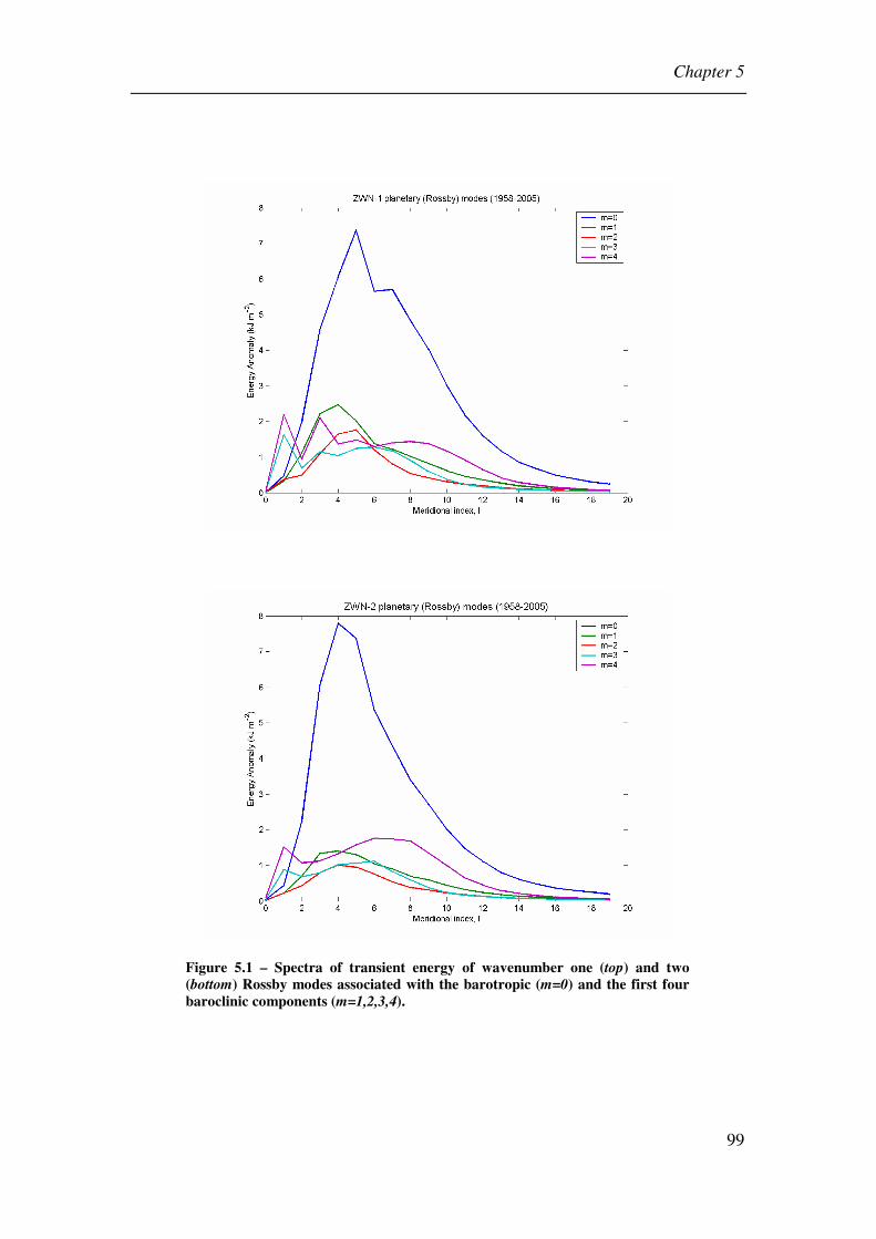
Chapter 5
99
Figure 5.1 – Spectra of transient energy of wavenumber one (top) and two (bottom) Rossby modes associated with the barotropic (m=0) and the first four baroclinic components (m=1,2,3,4).
Chapter 5
100
5.1.2. Variability of wave energy
Energy has been calculated for each wave, using Equation 3.7, without filtering the
coefficients and then restricting to low frequency waves, i.e. the coefficients were
filtered by a 15-day running mean that was applied before computing the energy.
Energy anomalies were computed following the method described on section 3.3.6.
Figure 5.2 represents the extended winter mean energy spectra of the Rossby modes
with wavenumbers s = 1 and 2, for the barotropic (Figure 5.2a) and first two
baroclinic modes m = 1, 2 (Figures 5.2b and 5.2c). Both the complete spectra and the
spectra for low frequency waves are presented and it may be observed that the
patterns of the spectra are similar, even though values are lower, as expected, in the
case of the filtered spetra.

Chapter 5
101
Figure 5.2 – Extended winter mean energy (1958 – 2005) of the Rossby modes with wavenumbers s = 1 and 2 associated with: (left page) barotropic (m = 0); and the first two baroclinic (top) m = 1 and (bottom) m = 2 structures. Both the complete spectra (solid blue) and the spectra for low frequency waves (dashed red) are represented for each wavenumber.
Chapter 5
102
The variability spectra, i.e. the spectra of the standard deviation of intraseasonal or
interannual anomalies (Figure 5.3) are similar to the respective spectra of the mean
energy. The barotropic modes represent the largest amount of energy, in agreement
with the fact that they are sensitive to the circulation of the largest fraction of the
atmospheric mass, the troposphere. The baroclinic modes m = 1, 2 are more sensitive
to the lighter layer of atmospheric mass, the stratosphere, and represent smaller
amounts of energy. A remarkable feature in the spectra of baroclinic (m = 1, 2) modes
is the large difference between the energy of wavenumbers s = 1 and s = 2, which is
to be attributed to the wavenumber filtering by the stratosphere.
Since we aim to relate time changes in the energy associated with planetary Rossby
waves with the observed vortex variability, we have projected the atmospheric
circulation onto the first 20 Rossby modes. Results shown in Figures 5.1 to 5.3 clearly
point out that the most important modes were indeed retained in our analysis.
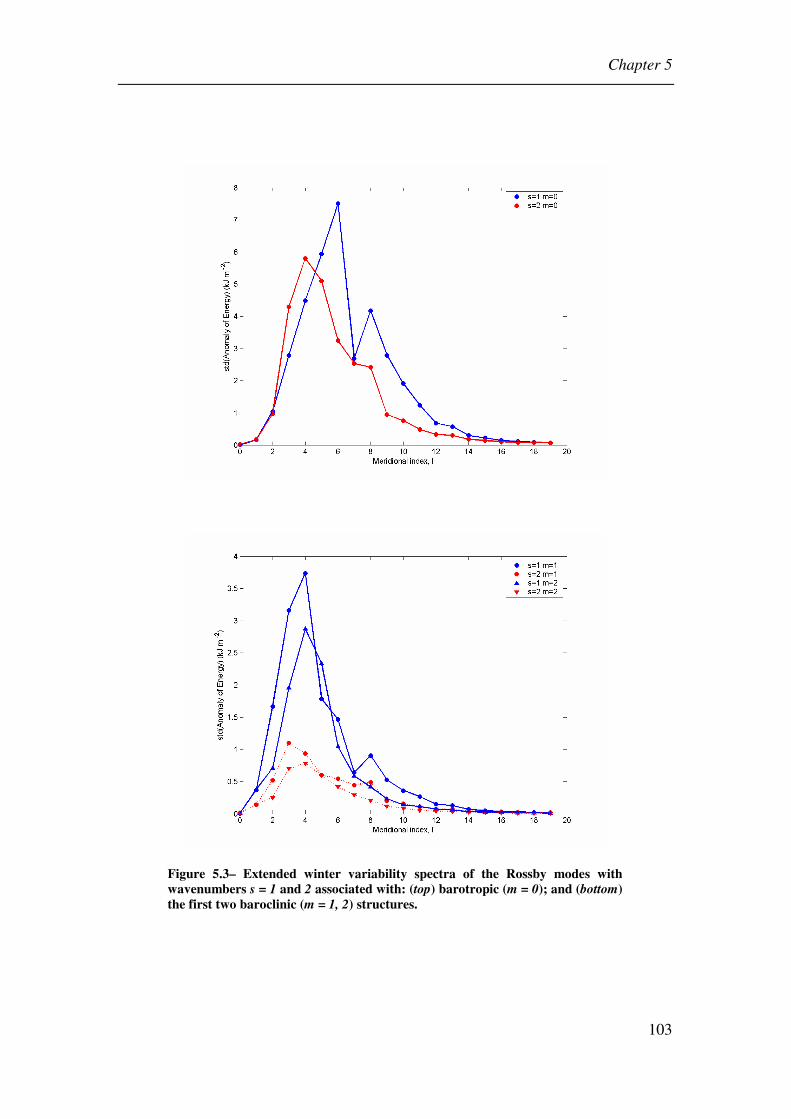
Chapter 5
103
Figure 5.3– Extended winter variability spectra of the Rossby modes with wavenumbers s = 1 and 2 associated with: (top) barotropic (m = 0); and (bottom) the first two baroclinic (m = 1, 2) structures.

Chapter 5
104
5.2. Study of Vortex Variability – the classical approach
Recently, a set of observational studies has focused on the daily evolution of strong
vortex anomalies [McDaniel and Black 2005], polar vortex intensification (VI)
[Limpasuvan et al. 2005], the life cycle of SSW events [Limpasuvan et al. 2004;
Nakagawa and Yamazaki 2006; Charlton and Polvani 2007] and the evolution of
SFW events [Black et al. 2006].
During boreal winter tropospheric NAM events are often preceded by variations in the
strength of the stratospheric polar vortex [Baldwin et al. 2003]. However, not all
NAM cases follow the statistical prototype of stratospheric initiation followed by
downward signal movement (hereafter referred to as downward “propagation”) into
the troposphere, as certain robust stratospheric NAM events are not associated with
corresponding succeeding tropospheric NAM events [Baldwin and Dunkerton 1999;
Zhou et al. 2002]. Accounting for such case to case variability represents an important
test of any theory regarding stratospheric influences upon tropospheric climate.
Black and McDaniel [2004] focused their study in identifying dynamical reasons why
some strong stratospheric NAM events do not extend downward to tropospheric
levels. Black and McDaniel’s [2004] results indicate important roles for both direct
and indirect forcing mechanisms in performing stratospheric influences upon
tropospheric climate. These authors conclude that whether or not a tropospheric NAM
signal emerges from a given stratospheric NAM event is largely dependent upon (1)
whether stratospheric PV anomalies descend to sufficiently low altitudes within the
stratosphere and (2) the detailed nature of any pre-existing zonally-symmetric
(annular) modes in the troposphere.
The statistical relation between the stratosphere and tropospheric circulation anomaly
patterns associated with the NAM on intraseasonal time scales has been studied
[Baldwin and Dunkerton 1999; Baldwin et al. 2003] but detailed diagnoses of the
dynamical processes leading to daily variability in the NAM are needed to fully
understand the mechanisms governing stratosphere-troposphere interaction. McDaniel
Chapter 5
105
and Black [2005] provide an observational study of the zonal wind tendency budget
for both the growth and decay stages of large amplitude positive and negative NAM
events. McDaniel and Black [2005] deduce the proximate forcings of the zonal mean
wind tendency during maturing and declining NAM stages employing transformed
eulerian mean, piecewise potential vorticity inversions, and regional Plumb flux
diagnoses. A remarkable degree of reverse symmetry is observed between the zonal-
mean dynamical evolution of positive and negative NAM events. Anomalous
equatorward and downward (poleward and upward) Eliassen-Palm fluxes are
observed during the maturation of positive (negative) NAM events, consistent with
index of refraction considerations and an indirect downward stratospheric influence.
The associated patterns of anomalous wave driving provide the primary forcing of the
zonal wind tendency field. Spectral analyses reveal that both the stratospheric and
tropospheric patterns of wave driving are primarily due to low frequency planetary
scale eddies.
Regional wave activity flux diagnoses further illustrate that this wave driving pattern
represents the zonal mean manifestation of planetary scale anomalies over the North
Atlantic that are linked to local anomalies in stationary wave forcing. The decay of
NAM events coincides with the collapse in the pattern of anomalous stationary wave
forcing over the North Atlantic region. McDaniel and Black’s [2005] diagnostic
results indicate that both (a) synoptic eddies and (b) direct downward stratospheric
forcing provide second order reinforcing contributions to the intraseasonal dynamical
evolution of NAM events.
Similar to past studies McDaniel and Black [2005] find that stratospheric variations in
the NAM are strongly driven by variations in upward propagating tropospheric
planetary scale waves [e.g., Hartmann et al. 2000; Limpasuvan et al. 2004].
McDaniel and Black [2005] reviewed several mechanisms that have been proposed to
explain stratosphere-troposphere coupling observed during the NAM. In one of the
mechanisms the stratosphere provides an indirect influence upon the troposphere.

Chapter 5
106
Specifically, changes in the vertical wind shear near the tropopause alter the index of
refraction which in turn alters the propagation of tropospheric Rossby waves [Chen
and Robinson 1992; Hartman et al. 2000]. During the positive (negative) phase of the
NAM, strong positive (negative) zonal-wind anomalies are observed in the
stratosphere at high latitudes (~65ºN) while negative (positive) zonal-wind anomalies
are observed in the mid-latitude (~35ºN) stratosphere. The associated vertical wind
shear is such that during the positive phase vertically propagating tropospheric
Rossby waves are deflected equatorward with less wave activity reaching the
stratospheric polar vortex. The reduction of wave breaking in the polar vortex results
in an anomalously strong polar jet, providing a positive feedback that tends to keep
the NAM in the positive phase. Meanwhile, the redirection of wave activity within the
troposphere provides anomalous wave driving signatures within the middle and upper
troposphere. Thus this mechanism provides an indirect stratospheric influence in
which tropospheric waves act to alter the tropospheric zonal wind field. This indirect
mechanism may affect the forcing and propagation characteristics of synoptic
[Polvani and Kushner 2002; Song and Robinson 2004] and planetary scale
tropospheric waves [DeWeaver and Nigam 2000; Hartmann et al. 2000].
Limpasuvan et al. [2004; 2005] have studied polar VI showing that the gross behavior
of VI events is similar in shape but opposite in sign to the one associated with SSW
events. A strong relationship exists between these midwinter weakenings in the polar
vortex, known as SSW events, and intraseasonal NAM variability [Limpasuvan et al.
2004].
In the NH, the linkage between the stratosphere and troposphere appears most
obvious when the stratospheric polar vortex undergoes unusually strong variation in
wind strength and temperature. Conditions of anomalously weak stratospheric polar
vortex are associated with SSW events in which the polar stratospheric temperature
rises dramatically over a short time period [e.g., McIntyre 1982; Andrews et al. 1987].
Quiroz [1977], O’Neill and Taylor [1979], and O’Neill [1980] first presented

Chapter 5
107
evidence for the appearance of near-surface temperature anomalies in conjunction
with the major NH SSW event of 1976–1977.
Kodera et al. [2000] have studied the relationship between SSW events and slowly
propagating zonal wind anomalies during the NH cold season (November to March)
using two leading EOF of 15-day mean zonal-mean zonal wind. They showed that
major SSW events occur in phase with the slowly propagating zonal wind anomalies,
which implies a “conditioning” of the atmosphere by the slowly varying state. These
authors also stress that changes in the tropospheric planetary waves associated with
the slowly propagating zonal wind anomalies coincide with changes in the AO. On
their figure 2 (here reproduced as Figure 5.4) they describe the anomaly progression
by the trajectory in the phase space of the first two EOF around the plane, at intervals
of 45º. The first EOF has large amplitude in the polar region of the upper stratosphere,
while the second EOF describes an inclined, dipole-type pattern: the positive pole is
located at the midlatitude stratopause, while the negative pole is located at high
latitudes in the middle stratosphere. According to the authors, Figure 5.4 illustrates
how movement around the phase angle φ describes the structure of downward and
poleward propagating wind anomalies in the stratosphere, which progress at a rate
proportional to the change in phase angle.
Figure 5.4 – Spatial structure of zonal winds corresponding to a different direction of a unit vector in a plane constructed by EOF 1 and EOF 2. Panels show patterns corresponding to one rotation from -135º to 180º. Number on each panel indicates an angle of rotation φφφφ in equation
( ) ( )cos 1 s 2P A EOF en EOFφ φ φ= ⋅ + ⋅ . EOF 1 and EOF 2 correspond to
phases φφφφ = 0º and 90º (as marked). Contour interval is 2.5 ms-1, and negative values are shaded (Figure 2 from Kodera et al. [2000]).
Chapter 5
108
Limpasuvan et al. [2004] noted that the composite SSW life cycle is preceded by
preconditioning of the upper stratospheric circulation and by anomalous planetary-
scale wave forcing at stratospheric and near-surface levels. As the SSW matures (and
the vortex becomes weaker), the largest stratospheric zonal flow and temperature
anomalies and the region of largest wave driving descend throughout the depth of the
stratosphere, as a result of wave mean flow interactions. When the anomalous wave
driving reaches the lowermost stratosphere, the associated flow anomalies appear to
penetrate the tropopause, drawing substantial anomalous responses in both wave
propagation and the mean meridional circulation at tropospheric levels [Haynes et al.
1991; Kuroda and Kodera 1999; Shindell et al. 1999a]. In contrast to the waves that
initiate the stratospheric warming, the anomalous tropospheric wave forcing during
the mature phase of the SSW is associated primarily with waves smaller than
planetary-scale.
Limpasuvan et al. [2004] also show (on their Figure 10) that strong heat flux
anomalies are observed in the preconditioned upper stratosphere several weeks before
the weakest state of the polar vortex. The heat fluxes are associated mainly with
quasi-stationary wavenumber 1 disturbances that are evident at both tropospheric and
stratospheric levels.
On a subsequent work, Limpasuvan et al. [2005] examined stratosphere-troposphere
evolution associated with polar VI events in the NH winter. These authors show that
incipient stage of a VI event is marked by anomalously low wave activity and
descending westerly anomalies over the depth of the polar stratosphere. Reduced
poleward planetary wave heat flux occurs as the circumpolar wind becomes stronger
and geopotential height anomalies penetrate toward the surface. The downward
progressing geopotential height anomaly patterns project strongly onto the positive
state of the NAM. Concurrently, anomalous poleward momentum flux develops in the
upper troposphere, and the related tropospheric mean meridional circulation provides
an easterly torque which maintains the wind anomalies reaching lower-troposphere
against surface drag. These authors argue that the gross behaviour of the composite VI

Chapter 5
109
event is similar in shape but opposite in sign to that associated with SSW events.
However, the descent of the wind and temperature anomalies over the VI life cycle is
generally weaker and slower than its SSW counterpart preceding the maximum vortex
anomaly. Similarly, after the maximum wind event, the weakening of the winds is
faster than the strengthening of the winds after a SSW. According to Limpasuvan et
al. [2005] this is because stratospheric wind reduction anomalies are produced by
wave driving, which can be rapid, and increases in wind speed are associated with the
radiative cooling of the polar cap, which happens more gradually. While the
contributions of the anomalous momentum fluxes by the quasi-stationary and synoptic
eddies are similar to SSWs, the much stronger anomalous momentum flux observed
during VI can be attributed to the larger role of eddies with timescales between 15 and
40 days and of wavenumber 2 scale. Notable differences between VI and SSW appear
in the tropical region. In particular, anomalous VI tends to occur more frequently
during La Niña conditions while most El Niño winters tend to be associated with
SSW events.
The factors affecting the downward propagation of SSW events to the troposphere
have also been studied by Nakagawa and Yamazaki [2006] through composite
analysis of 45-year reanalysis data from the ECMWF. The study distinguished two
types of SSW events: a wave-2 type SSW event and a wave-1 type SSW event.
During the growth stage of SSW, events that propagate into the troposphere exhibit
enhanced upward flux of the wavenumber two wave, while events that do not
propagate downward display reduced wavenumber two flux. In both events, upward
flux of the wavenumber one wave is enhanced, but the enhancement is stronger in the
non-propagating event. Nakagawa and Yamazaki’s [2006] composite for propagating
events reveals a negative Eurasian pattern of horizontal geopotential anomalies in the
troposphere during the growth stage, and a negative AO pattern following the event,
while non-propagating events are preceded by a positive Eurasian pattern. In both
types of events, the tropospheric anomalies are generated mainly by tropospheric
planetary wave forcing prior to the emergence of SSW.

Chapter 5
110
Since the discovery of SSW events by Scherhag [1952], many studies have examined
the dynamics of individual major warming events. However, only a few studies,
including those by Labitzke [1977] and Manney et al. [2005] have attempted to
establish a climatology of major, midwinter, SSW events. According to Charlton and
Polvani [2007] their study builds on those earlier works and is novel and distinctive in
three important respects. First, they provide full dating information for SSW events,
including the day of occurrence, and tabulate all events from the late 1950s to the
present. Second, their climatology is established based on two widely used reanalysis
datasets, which had not been previously examined for SSW activity. Third, these
authors use a new analysis technique that, for the first time, classifies the SSW events
into vortex displacement and splitting events.
Charlton and Polvani’s [2007] study is closely related to the one of Limpasuvan et al.
[2004]. However, while the latter used the 50-hPa annular mode to define SSW events
and considered only the NCEP–NCAR reanalysis dataset, Charlton and Polvani
[2007], using the WMO definition of SSW events (easterly winds at 10-hPa and
60°N), developed a more sophisticated algorithm and examined both the NCEP–
NCAR and the 40-yr ECMWF ReAnalysis (ERA-40) datasets in the extended winter
(November–March).
Using this new tool, they attempted to answer several key questions, in particular the
following ones:
• Are vortex displacements and vortex splits dynamically different? If so how?
• Do vortex displacements and vortex splits differ in their impacts on the
tropospheric flow?
They conclude that:
1) Vortex displacements and splits should be considered dynamically distinct.
Prior to vortex displacements and vortex splits, the vertical and horizontal
structure of the stratosphere and troposphere is different. In particular,

Chapter 5
111
anomalously strong zonal flow in the troposphere appears essential for the
occurrence of vortex splits. Vortex splits are accompanied by a significantly
anomalous flow in the Pacific sector. There is also clear evidence of early,
precursor wave activity for the vortex splits but not for vortex displacements.
2) While there are some differences in the spatial structures of the tropospheric
impact of vortex displacements and vortex splits, there is little difference in
the averaged tropospheric impact. This suggests that the mechanism for the
impact of the stratosphere on the tropospheric flow following major
stratospheric disturbances might have little dependence upon the precise
structure of anomalies in the lower stratosphere.
This work of Charlton and Polvani [2007] and their conclusions are relevant to this
study as we will be using their climatology in our analysis (Table 3.1 in section 3.3.4).
Moreover, we anticipate that our results will contribute to elucidate the problems
posed by the above-mentioned questions.
Black et al. [2006] studied the evolution of SFW events focusing on the relationship
between SFW events and the observed Northern extratropical circulation.
Specifically, SFW events are associated with a vertically coherent north-south dipole
pattern in the zonal wind anomaly field at mid to high latitudes. However, this pattern
is distinct from the canonical NAM structure as the primary centers in the north-south
anomaly dipole are retracted northward compared to the NAM. Results of Black et al.
[2006] indicate that SFW events may be associated with a distinct and previously
unrecognized intraseasonal annular mode of variability that strongly couples the
stratosphere and troposphere on submonthly time scales at mid to high latitudes (the
Polar Annular Mode – PAM). Black and McDaniel [2006] also found that the
evolution of SSW events is dominated by NAM variability whereas NAM and PAM
play approximately equal roles in SFW events.
The tropospheric anomaly patterns obtained by Black and McDaniel [2006] are more
strongly annular with relatively weak amplitudes over the North Atlantic. This

Chapter 5
112
suggests that, during periods of stratosphere-troposphere NAM coupling, the
tropospheric patterns have a substantial component that represents an internal
tropospheric response to stratospheric NAM variability [e.g., the indirect tropospheric
response discussed by McDaniel and Black 2005]. As such, Black and McDaniel’s
[2006] analysis provides a useful dynamical framework for delineating stratospheric
and tropospheric NAM variability. This separation also serves to isolate the direct
impact of the polar vortex variability upon the troposphere. Since stratospheric the
NAM and PAM events studied by these authors induce large-scale tropospheric
circulation anomaly patterns with similar amplitudes, Black and McDaniel [2006]
suggest that variations in the strength and position of the stratospheric polar vortex
each provide comparable direct effect to the tropospheric circulation. However, these
impacts have different spatial patterns and time scales.
The dynamical nature of wave driving field was explored by Black and McDaniel
[2006] by performing temporal and spatial decompositions of the input wave fields.
These analyses indicate that the anomalous wave driving signatures in both the
stratosphere and troposphere are mainly due to low frequency (intraseasonal periods
greater than 10 days) planetary scale (wavenumbers 1-3) eddies. The role of smaller
scale (wavenumbers 4 and higher) eddies is to provide secondary enhancements to the
upper tropospheric wave driving pattern near 60ºN. Further, zonal-mean analyses of
the regional wave activity flux field indicate that the composite anomaly field, itself,
is able to account for most of the low frequency planetary scale wave driving. This
suggests that the composite anomaly field contains the fundamental essence of the
intraseasonal dynamical evolution of the NAM.
5.3. Study of Vortex Variability – the energy perspective
In the above-mentioned studies as well as in many others, the analysis of the wave
forcing of the stratospheric polar vortex was performed within the traditional
framework of EP flux. However, the use of the EP flux as a diagnostic tool of wave

Chapter 5
113
propagation is strictly valid only in the case of small-amplitude waves. Frequent
usage is also made of other concepts associated with EP flux diagnostics, such as
refractive indices and critical lines, even though neither the Wentzel–Kramers–
Brillouin–Jeffries (WKBJ) approximation relating refractive indices and critical lines
to wave propagation nor the relation between wave propagation and EP flux are valid
in the case of strongly nonlinear flows like those that take place during SSW events
[Thuburn and Lagneau 1999].
To our knowledge no studies have considered the wave forcing of the stratospheric
polar vortex from the point of view of the energy associated with the forcing waves.
The main goal of this chapter is therefore to perform a diagnostic study of the total
(i.e. kinetic + available potential) energy associated with the planetary waves that
force the vortex dynamics. The analysis is based on a 3D normal mode decomposition
of the atmospheric global circulation, which is partitioned into planetary Rossby
waves and inertio–gravity waves, both types of waves possessing barotropic and
baroclinic vertical structures. Time changes in the energy associated with each wave
component may then be related with the observed vortex variability. It is worth
emphasizing that instead of being restricted to the extratropical region, the analysis is
here applied to the global atmosphere, and the circulation components are selected
based on 3D global functions. In this respect the connection between the polar
stratospheric variability and the QBO is worth being emphasized [Holton and Tan
1980; Labitzke 1982], together with the model results of Naito et al. [2003] that have
revealed a short-time cooling response to SSW events extending to the summer
hemisphere, a feature that suggests the global character of SSW events.
Another important feature of the method used here is that the energy is computed for
the total circulation (i.e. climatology + anomaly) and therefore energy anomalies,
associated with vortex variability, also include the contribution from the
climatological waves, which should be taken into account when performing
composite analysis.

Chapter 5
114
The fact that the 3D normal modes are eigensolutions of a set of primitive equations,
linearized with respect to a basic state at rest, may be pointed out as a shortcoming of
their use. However, the normal modes form a complete basis to expand the global
circulation, and the divergent or rotational character as well as the horizontal and
vertical structures of the circulation projected onto them do not depend on the
magnitude of the anomalies. On the other hand, as the normal mode approach allows
decomposing the circulation both into zonal and meridional scales, we may assess the
sensitivity of vortex wave forcing to both spatial scales. In this respect it is worth
recalling that the linear wave theory shows that the vertical wave propagation depends
both on zonal and meridional wavenumbers [Andrews et al. 1987]. However, EP flux
diagnostic studies found in the literature only show the dependence on the zonal scale
by means of Fourier decompositions.
5.3.1. Lagged correlations between the vortex strength and the wave
energy
As previously mentioned, Limpasuvan et al. [2004; 2005] have shown that the gross
behavior of VI events is similar in shape but opposite in sign to the one associated
with SSW events. It is therefore natural to analyze vortex forcing by means of lagged
correlations between stratospheric NAM indices and wave energy anomalies. A 15-
day running mean was applied to the NAM indices as well as to the total (i.e.
climatological + anomaly) atmospheric fields before computing the energy. This
procedure was motivated by the known fact that the stratospheric vortex is mainly
forced by stationary waves, but similar results were obtained when the 15-day running
average was applied after computing the energy, an indication of the negligible role
played by high-frequency waves in the process of vortex deceleration.
5.3.1.1. Zonal dependence
Results obtained for planetary Rossby waves of wavenumber s = 1 are shown in
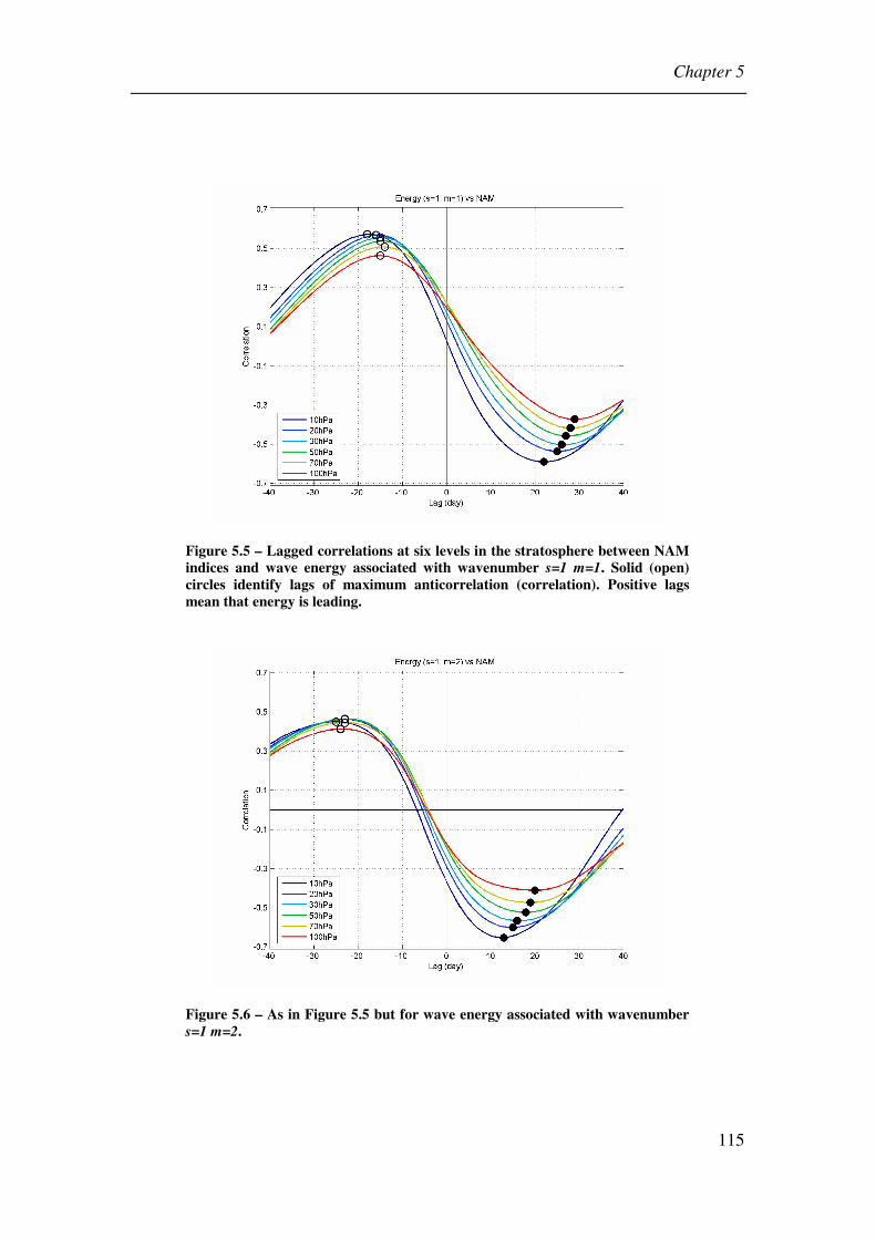
Chapter 5
115
Figure 5.5 – Lagged correlations at six levels in the stratosphere between NAM indices and wave energy associated with wavenumber s=1 m=1. Solid (open) circles identify lags of maximum anticorrelation (correlation). Positive lags mean that energy is leading.
Figure 5.6 – As in Figure 5.5 but for wave energy associated with wavenumber s=1 m=2.
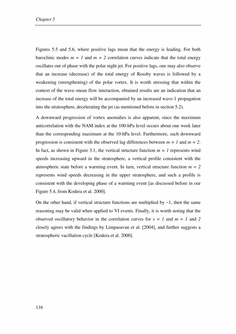
Chapter 5
116
Figures 5.5 and 5.6, where positive lags mean that the energy is leading. For both
baroclinic modes m = 1 and m = 2 correlation curves indicate that the total energy
oscillates out of phase with the polar night jet. For positive lags, one may also observe
that an increase (decrease) of the total energy of Rossby waves is followed by a
weakening (strengthening) of the polar vortex. It is worth stressing that within the
context of the wave–mean flow interaction, obtained results are an indication that an
increase of the total energy will be accompanied by an increased wave-1 propagation
into the stratosphere, decelerating the jet (as mentioned before in section 5.2).
A downward progression of vortex anomalies is also apparent, since the maximum
anticorrelation with the NAM index at the 100-hPa level occurs about one week later
than the corresponding maximum at the 10-hPa level. Furthermore, such downward
progression is consistent with the observed lag differences between m = 1 and m = 2.
In fact, as shown in Figure 3.1, the vertical structure function m = 1 represents wind
speeds increasing upward in the stratosphere, a vertical profile consistent with the
atmospheric state before a warming event. In turn, vertical structure function m = 2
represents wind speeds decreasing in the upper stratosphere, and such a profile is
consistent with the developing phase of a warming event [as discussed before in our
Figure 5.4, from Kodera et al. 2000].
On the other hand, if vertical structure functions are multiplied by −1, then the same
reasoning may be valid when applied to VI events. Finally, it is worth noting that the
observed oscillatory behavior in the correlation curves for s = 1 and m = 1 and 2
closely agrees with the findings by Limpasuvan et al. [2004], and further suggests a
stratospheric vacillation cycle [Kodera et al. 2000].

Chapter 5
117
5.3.1.2. Meridional dependence
As previously noted, the linear wave theory suggests that the vertical wave
propagation depends on both the zonal and the meridional wavenumbers [Andrews et
al. 1987]. However the lagged correlations that are depicted in Figures 5.5 and 5.6
refer to the sum of the energy of all meridional modes. To assess the effects due to the
meridional scales we computed the lagged correlations between the energy of each
Rossby mode and the vortex strength at the same stratospheric levels. Figures 5.7 and
5.8 show the obtained largest correlations or anticorrelations as a function of the
meridional index of the Rossby modes. It should be noted that the considered positive
(negative) lags lie inside the time intervals where the maximum anticorrelations
(correlations) in Figures 5.5 and 5.6 were found [i.e., the considered positive
(negative) lags are contained by the interval where curves in Figures 5.5 and 5.6 are
marked by solid (open) circles]. It is well apparent that the larger meridional scales
(i.e. the smaller meridional indices) are the only ones that significantly interact with
the vortex strength. As negative correlations were obtained when the energy was
leading the vortex strength (i.e. with positive lags) and therefore represent a forcing of
the vortex strength, it may seem awkward that the magnitude of the anticorrelations is
smaller for meridional indices l = 0, 1, and 2. However, such behavior is readily
understood if we take into account that the largest values (weights) of the first
meridional structures do appear at lower latitudes than those associated with high
meridional indices. In fact, since the weights of the meridional structures at high
latitudes increase as the meridional index increases [Longuet-Higgins 1968],
meridional modes l = 0, 1, and 2 (l = 3,…,6) are more sensitive to the atmospheric
circulation at lower (higher) latitudes. The meridional Rossby mode l = 8 of the
second baroclinic structure (Figure 5.8) also presents a conspicuous positive
correlation for positive lags, but positive energy anomalies in this mode may be also
associated with an upscale energy transfer to the modes that forces the vortex.

Chapter 5
118
Figure 5.7 – Lagged correlations between the energy associated to Rossby modes with wavenumber s=1 and baroclinic structure m=1 and the NAM indices at the same six levels in the stratosphere. Solid (dashed) curves show the largest anticorrelations or correlations for positive (negative) lags.
Figure 5.8 – As in Figure 5.7 but for wave energy associated with wavenumber s=1 m=2.
Chapter 5
119
As pointed out above, positive correlations in Figures 5.5 and 5.6 may reflect a
stratospheric vacillation (see also Figure 5.9), but since the vortex strength is leading,
such positive values may also be due to some other effect of the vortex. In this
respect, we note that the obtained maximum correlation for s = 1 and m = 1 (Figure
5.7) occurs for meridional indices l = 1 and 2, a feature that may be the result of
equatorward wave refraction during the strong vortex period.
Figure 5.9 – Time change in energy associated to Rossby modes with wavenumber s = 1 and baroclinic structure m = 2. Solid line represents the autocorrelation of the sum of energy associated with meridional indices l = 2, 3,
4 and 5. Dashed line represents the lagged correlations between the sum of energy of the same meridional indices and the energy of the Rossby mode with meridional index l = 8.
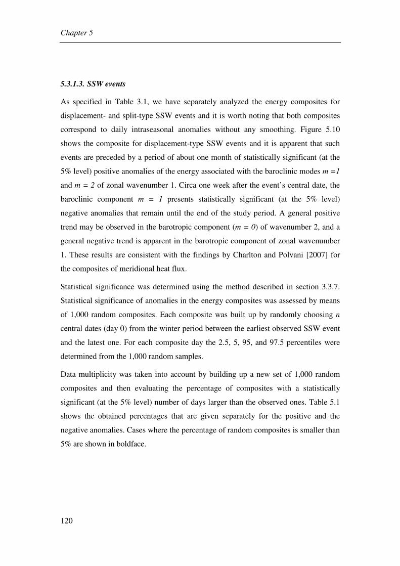
Chapter 5
120
5.3.1.3. SSW events
As specified in Table 3.1, we have separately analyzed the energy composites for
displacement- and split-type SSW events and it is worth noting that both composites
correspond to daily intraseasonal anomalies without any smoothing. Figure 5.10
shows the composite for displacement-type SSW events and it is apparent that such
events are preceded by a period of about one month of statistically significant (at the
5% level) positive anomalies of the energy associated with the baroclinic modes m =1
and m = 2 of zonal wavenumber 1. Circa one week after the event’s central date, the
baroclinic component m = 1 presents statistically significant (at the 5% level)
negative anomalies that remain until the end of the study period. A general positive
trend may be observed in the barotropic component (m = 0) of wavenumber 2, and a
general negative trend is apparent in the barotropic component of zonal wavenumber
1. These results are consistent with the findings by Charlton and Polvani [2007] for
the composites of meridional heat flux.
Statistical significance was determined using the method described in section 3.3.7.
Statistical significance of anomalies in the energy composites was assessed by means
of 1,000 random composites. Each composite was built up by randomly choosing n
central dates (day 0) from the winter period between the earliest observed SSW event
and the latest one. For each composite day the 2.5, 5, 95, and 97.5 percentiles were
determined from the 1,000 random samples.
Data multiplicity was taken into account by building up a new set of 1,000 random
composites and then evaluating the percentage of composites with a statistically
significant (at the 5% level) number of days larger than the observed ones. Table 5.1
shows the obtained percentages that are given separately for the positive and the
negative anomalies. Cases where the percentage of random composites is smaller than
5% are shown in boldface.

Chapter 5
121
Table 5.1 – Percentages of random composites that have a number of statistically significant (at 5% level) positive (negative) anomalies greater than the obtained number of statistically significant positive (negative) anomalies in the observed composite of displacement-type SSW events. Cases where the percentage of random composites is smaller than 5% are shown in boldface.
Positive Anomalies Negative Anomalies
m=0 m=1 m=2 m=0 m=1 m=2
s=1 100 0.0 0.0 100 0.7 6.0
s=2 100 100 100 38.3 100 100
As shown in Figure 5.11, composites for split-type SSW events suggest a different
dynamics from the ones of displacement-type SSW events. In this case both
wavenumbers 1 and 2 seem to play an important role and a precursor of such events,
associated with positive (negative) energy anomalies of the baroclinic m = 1
(barotropic m = 0) components of zonal wavenumber 1, seems to take place during
the period from about 30 to 15 days before the central date. It may be possible that
early wavenumber 1 energy anomalies are associated with a deceleration of the
stratospheric jet, setting the conditions for wavenumber 2 propagation into the polar
region. However, the present analysis cannot rule out the possibility of a downscale
energy transfer due to nonlinear wave interactions. Following such preconditioning,
split-type SSW events evolve with an increase of energy associated with the
barotropic and the baroclinic components of wavenumber 2, during a period of about
15 days before the event central’s date. Afterward, the baroclinic components of both
wavenumbers 1 and 2 present statistically significant (at the 5% confidence level)
negative anomalies. Finally, the observed drastic change in the sign of anomalies of
the barotropic component of wavenumber 2, from negative to positive lags, is
particularly worth noting since it gives an indication of drastic changes in the
energetics of the tropospheric circulation before and after the central dates of split-

Chapter 5
122
Figure 5.10 – Daily composites of intraseasonal anomalies of wave energy for SSW events of the displacement type (top s = 1; and bottom s = 2). Day 0 refers to the central date of the event. Solid (open) symbols identify mean values of intraseasonal anomalies that statistically differ from zero at the 5% (10%) significance level.
Chapter 5
123
Figure 5.11 – Daily composites of intraseasonal anomalies of wave energy for SSW events of the split type (top s = 1; and bottom s = 2). Day 0 refers to the central date of the event. Solid (open) symbols identify mean values of intraseasonal anomalies that statistically differ from zero at the 5% (10%) significance level.

Chapter 5
124
type SSW events. This result agrees with those of Nakagawa and Yamazaki [2006]
already described, who have shown that during the growth stage of SSW events that
propagate into the troposphere, there is an enhanced upward flux of energy associated
with wavenumber 2. Obtained results also support the findings of Charlton and
Polvani [2007] (see their conclusions – points 1 and 2 in section 5.2), but it is worth
stressing that our analysis points to the possible different nature of the tropospheric
impacts by displacement- and split-type SSW events.
Table 5.2 shows the statistical significance of the composites of split-type SSWs
taking into account data multiplicity.
Table 5.2 – Same as in Table 5.1, but for the split-type SSW events.
Positive Anomalies Negative Anomalies
m=0 m=1 m=2 m=0 m=1 m=2
s=1 53.7 1.3 20.9 38.0 0.0 4.1
s=2 2.1 0.8 1.0 2.7 9.9 0.1
5.3.2. SFW events
Figure 5.12 presents the energy composites that were obtained for the considered set
of the 19 earliest SFW events having occurred before 11 April. In case of zonal
wavenumber 1, it is well apparent that SFW events are preceded by statistically
significant (at the 5% level) positive energy anomalies of the first two baroclinic
components (m = 1 and 2), which concentrate into two distinct periods of time. This
feature is in strong agreement with the findings of Black et al. [2006] who have

Chapter 5
125
Figure 5.12 – Daily composites of intraseasonal anomalies of wave energy for SFW events (top s = 1; and bottom s = 2). Day 0 refers to the central date of the event. Solid (open) symbols identify mean values of intraseasonal anomalies that statistically differ from zero at the 5% (10%) significance level.

Chapter 5
126
identified two periods of strong vortex deceleration (see their Figure 2) that coincide
with two distinct bursts of upward EP flux (see their Figure 3). In particular it is worth
noting that the observed positive anomaly of the second baroclinic Rossby mode
during the second deceleration period (i.e. the time interval where the anomalies of
m= 2 are the only statistically significant ones) is also in agreement with the results of
Black et al. [2006]. Indeed, the second deceleration period in their Figure 2 is
characterized by easterly zonal mean zonal wind in the upper stratosphere and
westerly zonal wind in the lower stratosphere, a vertical structure that is well captured
by the baroclinic component m = 2. The statistical significance of the SFW
composites is shown in Table 5.3.
Table 5.3 – Same as in Table 5.1, but corresponding to SFW events.
Positive Anomalies Negative Anomalies
m=0 m=1 m=2 m=0 m=1 m=2
s=1 35.2 1.5 0.2 18.0 5.0 5.8
s=2 100 17.8 100 10.2 40.5 100
Finally, a comparison of Figures 5.10 and 5.12 suggests that the wave dynamics of
SFW events presents some similarities to the displacement-type SSW events. Both
events seem to be forced by means of an increase of energies associated with the
baroclinic Rossby modes (m = 1 and 2) of planetary wavenumber 1. Positive
anomalies of the energy are observed during the 30 days before the events, and there
is a trend of the energy associated with the barotropic Rossby mode of wavenumber 1
to decrease during the evolution of the events.

6. CONCLUSIONS
The annular nature of the leading patterns of the NH winter extratropical circulation
variability is revisited, and evidence is presented of the separation of both components
of annular and non-annular variability. The analysis relies on a PCA of tropospheric
geopotential height fields followed by lagged correlations of leading Principal
Components with the stratospheric polar vortex strength as well as with a proxy of
midlatitude tropospheric zonal mean zonal momentum anomalies.
Obtained results suggest that processes, occurring at two different times, may
contribute to the NAM spatial structure. Polar vortex anomalies appear positively
correlated with midlatitude tropospheric zonal mean zonal wind anomalies that occur
before the stratospheric anomalies. Following the polar vortex anomalies, zonal mean
zonal wind anomalies of the same sign are observed in the troposphere at high
latitudes. The time scale separation of the two signals is of about two weeks. As it is
well known, the PCA criterion for the identification of the leading PC is the
maximization of the represented data variability. Then, our results suggest that, in the
case of tropospheric circulation, that maximization is achieved with the variability
associated with the two above processes projecting on the leading EOF pattern. The
‘‘accumulation’’ or ‘‘deficit’’ of zonal mean zonal momentum at midlatitudes confers
the annular character to the leading patterns in those latitudes, and the ‘‘response’’ to
vortex variability confers the annularity at high latitudes.
To separate the processes discussed above, the geopotential height fields were linearly
regressed on the 500-hPa zonal mean zonal wind anomaly averaged in the latitudinal
band 45º–55ºN (U500 (45–55) index). Residual geopotential height fields were defined
as the geopotential height field minus the variability linearly regressed on the U500
(45–55) index. Then, a PCA of the residual geopotential fields was performed, and the
lagged correlations with the polar night jet were recalculated. It is worth noting that
subtracting the variability linearly dependent on the U500 (45-55) index does not
necessarily mean removing a dynamical zonally symmetric component. In fact, the
Chapter 6
128
correlation between the time series of the midlatitude (45º–55º N) zonal wind
strengths over the East Asia/Pacific sector (120ºE, 240º E) and over the Atlantic
sector (90ºW, 40ºE) is very close to zero (r = 0.02).
The leading EOF patterns of the residual variability, which seem to respond to the
vortex variability have a hemispheric scale but only show a dipolar structure over the
Atlantic basin like the NAO. The annularity of this pattern is clearly an imprint of the
Arctic center as referred by Deser [2000]. These findings agree with the results of
Feldstein and Franzke [2006] which suggest that neither the NAO events are confined
to the North Atlantic, nor NAM events are annular.
It is worth noting that the leading EOF patterns of the residual variability, which seem
to respond to the vortex variability, have a hemispheric scale showing only a dipolar
structure over the Atlantic basin that resembles NAO. These findings agree with the
results of Feldstein and Franzke [2006] which suggest that neither NAO events are
confined to the North Atlantic, nor NAM events are annular.
It is worth stressing that the separation of the two processes that contribute for
tropospheric NAM is especially relevant in studies of the tropospheric response to
changes originated in the stratosphere, e.g. changes in stratospheric chemical
composition and related global climate change. NAM indices represent zonally
symmetric zonal wind anomalies which spread from mid to high latitudes, whereas
the annularity of tropospheric response to stratospheric anomalies is confined to high
latitudes.
PCA was also applied to data that were previously filtered by means of a 3D normal
mode decomposition scheme of the atmospheric circulation, a procedure that allows
selecting both the most important zonal wavenumbers and meridional scales. For
instance Castanheira et al. [2002] have uncovered horizontal patterns of atmospheric
circulation variability by means of a PCA performed on the time series of the
projection coefficients.
Accordingly, a PCA was performed on the variability of the 31-day running averages

Chapter 6
129
of the barotropic zonally symmetric circulation of the NH for the cold season
(November-March). Leading EOF represents one half (50.4%) of the total variance,
which is statistically distinct from the remaining variability. The second EOF
represents 23.3% of the total variance. The daily time series of circulation anomalies
projected onto the leading EOF is highly correlated (r≥0.7) with the lower
stratosphere annular mode indices, showing that the annular variability extends from
the stratosphere deep into the troposphere. However, the analysis also reveals
differences between the zonally symmetric components of the annular modes defined
at single isobaric tropospheric levels (EOF1) and the meridional profile of EOF1 of
the barotropic zonally symmetric circulation. It is shown that the annular modes
defined at single isobaric tropospheric levels (EOF1) represent a much larger fraction
of zonally symmetric variability at midlatitudes than the one represented by the EOF1
of barotropic zonally symmetric circulation. The zonally symmetric component of the
500-hPa geopotential height regressed onto the lower stratosphere (70-hPa) NAM also
reveals the same differences with the zonally symmetric components of the annular
modes defined at single isobaric tropospheric levels (EOF1). Therefore it may be
concluded that a large fraction of midlatitude zonally symmetric variability, as
represented by the leading EOF at single isobaric tropospheric levels, is not linearly
associated with the stratospheric variability.
A PCA was also performed on the residual variability of 500-hPa geopotential that
remained after regressing out the 70-hPa NAM index. The leading EOF of such
variability reveals the PNA teleconnection pattern associated with a secondary wave
train over the Atlantic and Eurasia. The second EOF has a zonally symmetric
component similar to the one of the leading EOF of the total variability and is the
imprint of two meridional dipoles over the Pacific and the Atlantic oceans. Only a
very small fraction (less than 4%, |r| < 0.2) of the variability over each ocean basin is
correlated with the variability of the northern centre of the meridional dipole in the
opposite ocean basin. Results from the analysis of the 1000-hPa geopotential height
field are consistent with those from the analysis of the 500-hPa geopotential height

Chapter 6
130
field. The Pacific and Atlantic centres of the leading EOF of the 1000-hPa
geopotential height residual field do not belong to a common three-centre
teleconnection pattern. These results show that the midlatitude annular imprint on the
leading EOFs of the 500- and 1000-hPa geopotential height total fields is strongly
exaggerated by the PCA method, based on a criterion of maximizing the represented
variance integrated over the analyzed domain. In fact, the zonal mean zonal wind
anomalies over each northern ocean are positively correlated only at high latitudes.
No zonally symmetric coherent variability was found in the residual tropospheric
circulation. Hence the zonally symmetric coherent variability of the extratropical
tropospheric circulation appears to be always coupled with the stratospheric annular
variability. By construction, the leading EOF of the barotropic zonally symmetric
circulation explicitly takes this coupling into account. However, because the
barotropic component is approximately given by a vertical mass-weighted average of
the atmospheric circulation, it is much more sensitive to tropospheric variability. On
the other hand, the leading EOFs of total geopotential fields at single isobaric levels
show midlatitude zonally symmetric components which are strongly exaggerated by
variability due to local dynamics. This does not seem to be the case of the leading
EOF of the barotropic zonally symmetric circulation which represents a weaker
annular component in midlatitudes. Taken together, these results suggest that
projections onto the leading EOF of the barotropic zonally symmetric circulation may
provide a better index for the annular behaviour in the troposphere than projections
onto the leading EOFs of geopotential fields at single isobaric levels (NAM indices).
It is worth remarking again that tropospheric NAM indices do not seem to be
appropriate to represent the zonally symmetric circulation response to climate
changes. In fact, as already stressed, the zonally symmetric component of the leading
EOF of the isobaric geopotential height field in the troposphere is, at least to a great
extent, the imprint of independent dipolar structures over the ocean basins. These
results are particularly important for studies of the tropospheric response to changes
originating in the stratosphere, e.g. changes in stratospheric chemical composition.

Chapter 6
131
Use of indices based on the leading EOF of tropospheric geopotential height field
may in turn imply some artificial impact at midlatitudes.
We have also looked at the problem of the variability of the stratospheric polar vortex
from the point of view of planetary wave energetics. Our analysis differs from
traditional methods in that we have concentrated on a diagnosis of the energy
associated with the forcing waves instead of analyzing Eliassen–Palm fluxes. Another
difference from previous studies relates to the fact that instead of being restricted to
the extratropical subdomain, our analysis is applied to the whole atmosphere, and the
relevant circulation components are selected by means of projections onto 3D global
functions that allow partitioning the atmospheric (global) circulation into planetary
Rossby waves and inertio–gravity waves with barotropic and baroclinic vertical
structures.
We have found that positive (negative) anomalies of the energy associated with the
first two baroclinic Rossby modes m = 1 and m = 2 of planetary wave s = 1 are
followed by the downward progression of negative (positive) anomalies of the vortex
strength. A signature of the vortex vacillation is also well apparent in the lagged
correlation curves between the wave energy and the vortex strength. The analysis of
the correlations between individual Rossby modes and the vortex strength further
confirmed the result from linear theory that the waves that force the vortex are those
associated with the largest zonal and meridional scales.
Composites of SSW events of both displacement- and split-types were finally
analysed, revealing different dynamics. Displacement-type SSW events are forced by
positive anomalies of the energy associated with the first two baroclinic Rossby
modes m = 1 and m = 2 of planetary zonal wavenumber s = 1. On the other hand,
split-type SSW events are forced by positive anomalies of the energy associated with
planetary zonal wavenumber s = 2. Besides, the barotropic Rossby component of
wavenumber s = 2 has revealed a strong anomaly signal of opposite sign before and
after the central date of the event, suggesting that the tropospheric circulation plays an

Chapter 6
132
important role in the activation of split-type SSW events, and that, after the events,
anomalies propagate down to the troposphere [Nakagawa and Yamazaki 2006]. In the
case of split-type SSW events, a preconditioning of the stratospheric circulation seems
to take place three weeks before the event as suggested by the observed behaviour of
the anomalies of the baroclinic Rossby modes of zonal wavenumber s = 1. In the case
of SFW events, obtained results closely agree with the findings of Black et al. [2006]
and there is evidence that composites of SFW events exhibit an overall similar
behaviour to the ones observed in composites of the displacement-type SSW events.

REFERENCES
Ambaum, M. H. P., and B. J. Hoskins, 2002: The NAO Troposphere-Stratosphere
Connection. J. Climate, 15, 1969–1978.
Ambaum, M. H. P., B. J. Hoskins, and D. B. Stephenson, 2001: Arctic Oscillation or
North Atlantic Oscillation? J. Climate, 14, 3495–3507.
Andrews, D. G., J. R. Holton, and C. B. Leovy, 1987: Middle Atmosphere Dynamics.
Academic Press, 489 pp.
Baldwin, M. P., and T. J. Dunkerton, 2001: Stratospheric harbingers of anomalous
weather regimes. Science, 294, 581–584.
Baldwin, M. P., D. B. Stephenson, D. W. J. Thompson, T. J. Dunkerton, A. J.
Charlton, and A. O’Neill, 2003: Stratospheric Memory and Skill of Extended-Range
Weather Forecasts. Science, 301, 636–640.
Baldwin, M. P., X. Cheng and T. J. Dunkerton, 1994: Observed correlations between
winter-mean tropospheric and stratospheric circulation anomalies, Geophys. Res.
Lett., 21, 1141–1144.
Baldwin, M. P., and T.J. Dunkerton, 1999: Propagation of the Arctic Oscillation from
the stratosphere to the troposphere. J. Geophys. Res., 104, 30937–30946.
Barnett, T. P., 1985: Variations in near-global sea level pressure. J. Atmos. Sci., 42,
478–501.
Barnston, A. G., and R. E. Livezey, 1987: Classification, seasonality, and persistence
of the low-frequency atmospheric circulation patterns. Mon. Wea. Rev., 115, 1083–
1126.
Bjerknes, J. , 1969: Atmospheric teleconnections from the equatorial Pacific, Mon.
Wea. Rev., 97, 163–172.
Black, R. X., 2002: Stratospheric forcing of surface climate in the Arctic Oscillation.
J. Climate, 15, 268–277.

References
134
Black, R. X., B. A. McDaniel, and W. A. Robinson, 2006: Stratosphere–troposphere
coupling during spring onset. J. Climate, 19, 4891–4901.
Black, R. X., and B.A. McDaniel, 2004: Diagnostic case studies of the Northern
Annular Mode. J. Climate, 17, 3990-4004.
Black, R. X., and B. A. McDaniel, 2006: The Polar Annular Mode: Submonthly
Stratosphere-Troposphere coupling in the Arctic. Geophys. Res. Lett. (submitted).
Bretherton, C. S., C. Smith, and J. M. Wallace, 1992: An intercomparison of methods
for finding coupled patterns in climate data. J. Climate, 5, 541–560.
Castanheira J. M., M. L. R. Liberato, L. de la Torre, H.-F. Graf, and A. Rocha, 2008:
Annular versus non-annular variability of the Northern Hemisphere atmospheric
circulation. J. Climate (in press, accepted on 07/12/2007).
Castanheira, J. M., 2000: Climatic variability of the atmospheric circulation at the
global scale. Ph. D. Thesis, University of Aveiro, Portugal, 186 pp.
Castanheira, J. M., and H.-F. Graf, 2003: North Pacific–North Atlantic relationships
under stratospheric control? J. Geophys. Res., 108, 4036–4045,
doi:10.1029/2002JD002754.
Castanheira, J. M., C. C. DaCamara, and A. Rocha, 1999: Numerical solutions of the
vertical structure equation and associated energetics. Tellus, 51A, 337–348.
Castanheira, J. M., H.-F. Graf, C. DaCamara, and A. Rocha, 2002: Using a physical
reference frame to study global circulation variability. J. Atmos. Sci., 59, 1490–1501.
Castanheira, J. M., M. L. R. Liberato, C. A. F. Marques, and H.-F. Graf, 2007:
Bridging the Annular Mode and North Atlantic Oscillation paradigms. J. Geophys.
Res., 112, D19103, doi:10.1029/2007JD008477.
Charlton, A. J., and L. M. Polvani, 2007: A new look at stratospheric sudden
warmings. Part I: Climatology and modelling benchmarks. J. Climate, 20, 449–469.
Charney, J. G., and P. G. Drazin, 1961: Propagation of planetary-scale disturbances

References
135
from the lower into the upper atmosphere. J. Geophys. Res., 66, 83–109.
Chen, P., and W. A. Robinson, 1992: Propagation of planetary waves between the
troposphere and stratosphere. J. Atmos. Sci., 49, 2533–2545.
Cheng, X., and T. J. Dunkerton, 1995: Orthogonal rotation of spatial patterns derived
from singular value decomposition analysis. J. Climate, 8, 2631–2643.
Christiansen, B., 2001: Downward propagation of zonal mean zonal wind anomalies
from the stratosphere to the troposphere: Model and reanalysis. J. Geophys. Res., 106,
27307–27322.
Christiansen, B., 2002: On the physical nature of the Arctic Oscillation. Geophys.
Res. Lett., 29 (16), 10.1029/2002GL015208.
Daley, R., 1991: Atmospheric Data Analysis. Cambridge University Press, 457 pp.
Deser, C., 2000: On the teleconnectivity of the "Arctic Oscillation". Geophys. Res.
Lett., 27, 779–782.
DeWeaver E., and S. Nigam, 2000: Do stationary waves drive the zonal-mean jet
anomalies of the northern winter? J. Climate, 13, 2160–2176.
Dickinson, R. E., 1968: Planetary Rossby Waves Propagating Vertically Through
Weak Westerly Wind Wave Guides. J. Atmos. Sci., 25, 984–1002.
Dole, R. M., 1986: Persistent anomalies of the extratropical Northern Hemisphere
wintertime circulation: Structure. Mon. Wea. Rev., 114, 178–207.
Dommenget, D. and M. Latif, 2002: A Cautionary Note on the Interpretation of EOF.
J. Climate, 15, 216–225.
Eichelberger, S. J., and J. R. Holton, 2002:, A mechanistic model of the northern
annular mode, J. Geophys. Res., 107(D19), 4388, doi:10.1029/2001JD001092
Feldstein, S. B., 2000: Is interannual zonal mean flow variability simply climate
noise? J. Climate, 13, 2356–2362.
Feldstein, S. B., 2000: The timescale, power spectra, and climate noise properties of

References
136
teleconnection patterns. J. Climate, 13, 4430–4440.
Feldstein, S. B., and C. Franzke, 2006: Are the North Atlantic Oscillation and the
Northern Annular Mode Distinguishable? J. Atmos. Sci., 63, 2915–2930.
Feldstein, S. B., and W. A. Robinson, 1994: Comments on ‘Spatial structure of ultra-
low frequency variability of the flow in a simple atmospheric circulation model.’
Quart. J. Roy. Meteor. Soc., 120, 739–745.
Geller, M.A., and J.C. Alpert, 1980: Planetary wave coupling between the
Troposphere and the Middle Atmosphere as a possible sun-weather mechanism. J.
Atmos. Sci., 37, 1197–1215.
Gerber, E. P., and G. K. Vallis, 2005: A stochastic model for the spatial structure of
annular pattern of variability and the North Atlantic Oscillation. J. Climate, 18, 2102–
2118.
Glowienka-Hense, R., 1990: The North Atlantic Oscillation in the Atlantic-European
SLP. Tellus, 42A, 497–507.
Gong, D., and S. Wang, 1999: Definition of the Antarctic oscillation index. Geophys.
Res. Lett., 26, 459–462.
Graf, H.-F., J. Perlwitz, and I. Kirchner, 1994: Northern Hemisphere tropospheric
mid-latitude circulation after violent volcanic eruptions, Contr. Atm. Phys., 67, 3–13.
Graf, H.-F., J. Perlwitz, I. Kirchner, and I. Schult, 1995: Recent northern winter
climate trends, ozone changes, and increased greenhouse forcing. Contrib. Atmos.
Phys., 68, 233–248.
Hartmann, D. L., J. M. Wallace, V. Limpasuvan, D. W. J. Thompson, and J. R.
Holton, 2000: Can ozone depletion and global warming interact to produce rapid
climate change? Proc. Natl. Acad. Sci. USA, 97, 1412–1417.
Haynes, P. H., 2005: Stratospheric dynamics. Ann. Rev. Fluid Mech., 37,263–293.
Haynes, P. H., C. J. Marks, M. E. McIntyre, T. G. Shepherd, and K. P. Shine, 1991:

References
137
On the ‘‘downward control’’ of extratropical diabatic circulations by eddy-induced
mean zonal forces. J. Atmos. Sci., 48, 651–679.
Hines, C. O., 1974: A possible mechanism for the production of sun-weather
correlations. J. Atmos. Sci., 31, 589–591.
Holton J. R., P. H. Haynes, M. E. McIntyre, A. R. Douglass, R. B. Rood, L. Pfister,
1995: Stratosphere–troposphere exchange. Rev. Geophys., 33, 403–39.
Holton, J. R., 1976: Semi-spectral numerical-model for wave-mean flow interactions
in stratosphere – application to sudden stratospheric warmings. J. Atmos. Sci., 33,
1639–1649.
Holton, J. R., and C. Mass, 1976: Stratospheric vacillation cycles. J. Atmos. Sci., 33,
2218–2225.
Holton, J. R., and H.-C. Tan, 1980: The influence of the equatorial quasi-biennal
oscillation on the global circulation at 50 mb. J. Atmos. Sci., 37, 2200–2208.
Honda, M., and H. Nakamura, 2001: Interannual Seesaw between the Aleutian and
Icelandic Lows. Part II: Its Significance in the Interannual Variability over the
Wintertime Northern Hemisphere. J. Climate, 14, 4512–4529.
Horel, J. D., and J. M. Wallace, 1981: Planetary-scale atmospheric phenomena
associated with the Southern Oscillation. Mon. Wea. Rev., 109, 813–829.
Hoskins, B. J., and D. Karoly, 1981: The steady linear response of a spherical
atmosphere to thermal and orographic forcing. J. Atmos. Sci., 38, 1179–1196.
Hurrell, J. W., 1995: Decadal trends in the North Atlantic Oscillation: Regional
temperatures and precipitation, Science, 269, 676-679.
Hurrell, J. W., 1996: Influence of variations in extratropical wintertime
teleconnections on Northern Hemisphere temperature, Geophys. Res. Lett., 83,
665-668.
Jolliffe, I. T., 1986: Principal Component Analysis. Springer-Verlag, 290 pp.
References
138
Juckes M. N. , and M. E. McIntyre, 1987: A high resolution, one-layer model of
breaking planetary waves in the stratosphere. Nature, 328, 590–596.
Kalnay, E., and Coauthors, 1996: The NCEP/NCAR 40-Year Reanalysis Project.
Bull. Amer. Meteor. Soc., 77, 437–471.
Kasahara, A., and K. Puri, 1981: Spectral representation of three-dimensional global
data by expansion in normal mode functions. Mon. Wea. Rev. 109, 37–51.
Kistler R., and Coauthors, 2001: The NCEP–NCAR 50-Year Reanalysis: Monthly
means CD-ROM documentation. Bull. Amer. Meteor. Soc., 82, 247–267.
Kitoh, A., H. Koide, K. Kodera, S. Yukimoto and A. Noda, 1996: Interannual
variability in the stratospheric-tropospheric circulation in a coupled ocean-atmosphere
GCM, Geophys. Res. Lett., 23, 543-546.
Kodera, K., 1993: Quasi-Decadal Modulation of the Influence of the Equatorial
Quasi-Biennial Oscillation on the North Polar Stratospheric Temperatures, J.
Geophys. Res., 98(D4), 7245–7250.
Kodera, K., 1994: Influence of volcanic eruptions on the troposphere through
stratospheric dynamical processes in the Northern Hemisphere winter. J. Geophys.
Res., 99, 1273–1282.
Kodera, K., and H. Koide, 1997: Spatial and seasonal characteristics of recent decadal
trends in the northern hemisphere troposphere and stratosphere. J. Geophys. Res.,
102, 19433–19447.
Kodera, K., and K. Yamazaki, 1994: A possible influence of recent polar stratospheric
coolings on the troposphere in the Northern Hemisphere winter, Geophys. Res. Lett.,
21, 809–812.
Kodera, K., H. Koide, and H. Yoshimura, 1999: Northern Hemisphere winter
circulation associated with the North Atlantic Circulation and the stratospheric polar-
night jet, Geophys. Res. Lett., 26, 443–446.
References
139
Kodera, K., M. Chiba, H. Koide, A. Kitoh, and Y. Nikaidou, 1996: Interannual
variability of the winter stratosphere and troposphere in the Northern Hemisphere. J.
Met. Soc. Japan, 74, 365–382.
Kodera, K., Y. Kuroda, and S. Pawson, 2000: Stratospheric sudden warmings and
slowly propagating zonal mean zonal wind anomalies. J. Geophys. Res., 105, 12 351–
12 359.
Kuroda Y., and K. Kodera, 1999: Role of planetary waves in the stratosphere–
troposphere coupled variability in the Northern Hemisphere winter. Geophys. Res.
Lett, 26, 2375–2378.
Kushnir, Y., and J. M. Wallace, 1989: Low-frequency variability in the Northern
Hemisphere winter: Geographical distribution, structure and time-scale dependence. J.
Atmos. Sci., 46, 3122–3142.
Kutzbach, J. E., 1970: Large-scale features of monthly mean Northern Hemisphere
anomaly maps of sea-level pressure, Mon. Wea. Rev., 98, 708–716.
Kutzbach, J., 1967: Empirical eigenvectors of sea level pressure, surface temperature,
and precipitation complexes over North America. J. Appl. Meteor., 6, 791–802.
Labitzke, K., 1977: Interannual Variability of the Winter Stratosphere in the Northern
Hemisphere. Mon. Wea. Rev., 105, 762–770.
Labitzke, K., 1982: On the interannual variability of the middle stratosphere during
the northern winters. J. Meteor. Soc. Japan, 60, 124–139.
Leith, C. E., 1973: The standard error of time-average estimates of climatic means. J.
Appl. Meteor., 12, 1066–1069.
Liberato, M.L.R., J.M. Castanheira, L. de la Torre, C.C. DaCamara, and L. Gimeno,
2007: Wave Energy Associated with the Variability of the Stratospheric Polar Vortex.
J. Atmos. Sci., 64, 2683–2694.
Limpasuvan, V., D. L. Hartmann, D. W. J. Thompson, K. Jeev, and Y. L. Yung, 2005:

References
140
Stratosphere-troposphere evolution during polar vortex intensification. J. Geophys.
Res., 110, D24101, doi:10.1029/2005JD006302.
Limpasuvan, V., D. W. J. Thompson, and D. L. Hartmann, 2004: The life cycle of the
Northern Hemisphere sudden stratospheric warmings. J. Climate, 17, 2584–2596.
Livezey, R. E., and W. Chen, 1983: Statistical Field Significance and its
Determination by Monte Carlo Techniques. Mon. Wea. Rev., 111, 46–59.
Longuet-Higgins, M. S., 1968: The eigenfunctions of Laplace’s tidal equations over a
sphere. Philos. Trans. Roy. Soc. London, A262, 511–607.
Lorenz, E. N., 1951: Seasonal and irregular variations of the Northern Hemisphere
sea-level pressure profile. J. Atmos. Sci., 8, 52–59.
Lorenz, E. N., 1956: Empirical orthogonal functions and statistical weather
prediction, Rep. 1, Statist. Forecasting Project, MIT, 49pp.
Madden, R. A., 1976: Estimates of the natural variability of time averaged sea level
pressure. Mon. Wea. Rev., 104, 942–952.
Manney, G. L., K. Kruger, J. L. Sabutis, S. A. Sena, and S. Pawson, 2005: The
remarkable 2003–2004 winter and other recent warm winters in the Arctic
stratosphere since the late 1990s. J. Geophys. Res., 110, D04107,
doi:10.1029/2004JD005367.
Nakamura, H., M. Tanaka, and J. M. Wallace, 1987: Horizontal structure and
energetics of Northern Hemisphere winter teleconnection patterns. J. Atmos. Sci., 44,
3377–3391.
Mantua, N., S. Hare, Y. Zhang, J. Wallace, and R. C. Francis, 1997: A Pacific
interdecadal climate oscillation with impacts on salmon production. Bull. Amer.
Meteor. Soc., 78, 1069–1079.
Matsuno, T., 1970: Vertical Propagation of Stationary Planetary Waves in the Winter
Northern Hemisphere. J. Atmos. Sci., 27, 871–883.
References
141
Matsuno, T., 1971: A dynamical model of the stratospheric sudden warming. J.
Atmos. Sci., 28, 1479–1494.
McDaniel, B. A., and R. X. Black, 2005: Intraseasonal dynamical evolution of the
Northern Annular Mode. J. Climate, 18, 3820–3839.
McIntyre M. E., 1982: How well do we understand the dynamics of stratospheric
warmings? J. Meteorol. Soc. Japan, 60, 37–65.
McIntyre M. E., 2003a: Balanced flow. In Encyclopedia of Atmospheric Sciences,
vol. 2, ed. JR Holton, JA Pyle, JA Curry. London: Academic/Elsevier.
McIntyre M. E., 2003b: Potential vorticity. In Encyclopedia of Atmospheric Sciences,
vol. 2, ed. JR Holton, JA Pyle, JA Curry. London: Academic/Elsevier.
McIntyre M. E., and T. N. Palmer, 1983: Breaking planetary waves in the
stratosphere. Nature, 305, 593–600.
McIntyre M. E., and T. N. Palmer, 1984: The “surf zone” in the stratosphere. J.
Atmos. Terr. Phys., 46, 825–849.
Mo, K. C., and M. Ghil, 1987: Statistics and Dynamics of Persistent Anomalies. J.
Atmos. Sci., 44, 877–902.
Mo, K. C., and R. E. Livezey, 1986: Tropical–extratropical geopotential height
teleconnections during the Northern Hemisphere winter. Mon. Wea. Rev., 114, 2488–
2515.
Monahan, A. H., and J. C. Fyfe, 2006: On the Nature of Zonal Jet EOFs. J. Climate,
19, 6409–6424.
Monahan, A. H., L. Pandolfo, and J. C. Fyfe, 2001: The preferred structure of
variability of the Northern Hemisphere atmospheric circulation, Geophys. Res. Lett.,
28, 1019–1022.
Naito, Y., M. Taguchi, and S. Yoden, 2003: A parameter sweep experiment on the
effects of the equatorial QBO on stratospheric sudden warmings events. J. Atmos.

References
142
Sci., 60, 1380–1394.
Nakagawa, K. I., and K. Yamazaki, 2006: What kind of stratospheric sudden warming
propagates to the troposphere? Geophys. Res. Lett., 33, L04801,
doi:1029/2005GL024784.
North, G. R., 1984: Empirical orthogonal functions and normal modes. J. Atmos. Sci.,
41, 879–887.
North, G. R., T. L. Bell, R. F. Cahalan, and F. J. Moeng, 1982: Sampling errors in the
estimation of empirical orthogonal functions, Mon. Wea. Rev., 110, 699–706.
O’Neill, A., 1980: The dynamics of stratospheric warmings generated by a general
circulation model of the troposphere and stratosphere. Quart. J. Roy. Meteor. Soc.,
106, 659–690.
O’Neill, A., 2003: Stratospheric sudden warmings. Encyclopedia of Atmospheric
Sciences, J. R. Holton, J. A. Pyle, and J. A. Curry, Eds., Elsevier, 1342–1353.
Obukhov, A. M., 1947: Statistically homogeneous fields on a sphere. Ups. Mat.
Navk., 2, 196–198.
Perlwitz J., and N. Harnik, 2003: Observational evidence of a stratospheric influence
on the troposphere by planetary wave reflection. J. Climate, 16, 3011–3026.
Perlwitz, J., and H.-F. Graf, 1995: The statistical connection between tropospheric
and stratospheric circulation of the Northern Hemisphere in winter. J. Climate, 8,
2281–2295.
Perlwitz, J., and H.-F. Graf, 2001a: Troposphere-stratosphere dynamic coupling under
strong and weak polar vortex conditions. Geophys. Res. Lett., 28, 271–274.
Perlwitz, J., and H.-F. Graf, 2001b: The variability of the horizontal circulation in the
troposphere and stratosphere: A comparison. Theor. Appl. Clim., 69, 149–161.
Perlwitz, J., and N. Harnik, 2004: Downward coupling between the stratosphere and
troposphere: The relative roles of wave and zonal mean processes. J. Climate, 17,

References
143
4902–4909.
Plumb, R. A., and K. Semeniuk, 2003: Downward migration of extratropical zonal
wind anomalies. J. Geophys. Res., 108, 4223, (doi:10.1029/2002JD002773).
Polvani, L. M., and D. W. Waugh, 2004: Upward wave activity flux as a precursor to
extreme stratospheric events and subsequent anomalous surface weather regimes. J.
Climate, 17, 3548–3554.
Polvani, L. M., and P. J. Kushner, 2002: Tropospheric response to stratospheric
perturbations in a relatively simple general circulation model. Geophys. Res. Lett., 29,
1114, doi:10.1029/2001GL014284.
Preisendorfer, R. W., 1988: Principal Component Analysis in Meteorology and
Oceanography. Elsevier, 425 pp.
Quadrelli, R., and J. M. Wallace, 2004a: A simplified linear framework for
interpreting patterns of Northern Hemisphere wintertime climate variability. J.
Climate, 17, 3728–3742.
Quadrelli, R., and J. M. Wallace, 2004b: Varied expressions of the hemispheric
circulation observed in association with contrasting polarities of prescribed patterns of
variability. J. Climate, 17, 4245–4253.
Quiroz, R. S., 1977: Tropospheric-stratospheric polar vortex breakdown of January
1977, Geophys. Res. Lett., 4, 151–154.
Reyers, M., U. Ulbrich, M. Christoph, J. Pinto, and M. Kerschgens, 2006: A
mechanism of PNA influence on NAO. Geophysical Research Abstracts, Vol. 8,
10703, 2006, SRef-ID: 1607-7962/gra/EGU06-A-10703.
Richman, M. B., 1986: Rotation of principal components. J. Climatol., 6, 293–335.
Robock A., 2000: Volcanic eruptions and climate. Rev. Geophys., 38, 191–219.
Robock, A., and J. Mao, 1992: Winter warming from large volcanic eruptions,
Geophys. Res. Lett., 12, 2405–2408.

References
144
Rogers, J. C., and E.-M. Thompson, 1995: Atlantic Arctic cyclones and the mild
Siberian winters of the 1980s, Geophys. Res. Lett., 22, 799–802.
Rossby, C.-G. 1939: Relations between variations in the intensity of the zonal
circulation of the atmosphere and displacements of the semipermanent centers of
action. J. Mar. Res., 2, 38–55.
Schmitz, G., and N. Grieger, 1980: Model calculations on the structure of planetary
waves in the upper troposphere and lower stratosphere as a function of the wind field
in the upper stratosphere. Tellus, 32, 207–214.
Scott, R. K., P. H. Haynes, 1998: Internal interannual variability of the extratropical
stratospheric circulation: The low-latitude flywheel. Q. J. Roy. Meteor. Soc., 124,
2149–2173.
Scherhag, R., 1952: Die explosionsartigen Stratosphärenerwärmungen des
Spätwinters 1951–52. Ber. Dtsch. Wetterdienst (USZone), 6, 51–63.
Schubert, S. D., 1986: The structure, energetics and evolution of the dominant
frequency-dependent three-dimensional atmospheric modes. J. Atmos. Sci., 43, 1210–
1237.
Shindell, D. T., R. L. Miller, G. A. Schmidt, and L. Pandolfo, 1999a: Simulation of
recent northern winter climate trends by greenhouse-gas forcing, Nature, 399, 452–
455.
Shindell, D. T., D. Rind, N. Balachandran, J. Lean, and P. Lonergan, 1999b: Solar
cycle variability, ozone and climate. Science, 284, 305–308 ,
doi:10.1126/science.284.5412.305.
Simmons, A. J., J. M. Wallace and G. W. Branstator, 1983: Barotropic wave
propagation and instability, and atmospheric teleconnection patterns. J. Atmos. Sci.,
40, 1363–1392.
Song, Y., and W. A. Robinson, 2004: Dynamical mechanisms for stratospheric
influences on the troposphere. J. Atmos. Sci., 61, 1711–1725.
References
145
Tanaka H. L., Y. Watarai, and T. Kanda, 2004: Energy spectrum proportional to the
squared phase speed of Rossby modes in the general circulation of the atmosphere,
Geophys. Res. Lett., 31 (13), L13109, doi:10.1029/2004GL019826.
Tanaka, H. L., 1985: Global energetics analysis by expansion into three dimensional
normal mode functions during the FGGE winter. J. Meteor. Soc. Japan, 63, 180–200.
Tanaka, H. L., 2003: Analysis and modeling of the Arctic Oscillation using a simple
barotropic model with baroclinic eddy forcing. J. Atmos. Sci., 60, 1359–1379.
Tanaka, H. L., and Q. Ji, 1995: Comparative energetics of FGGE Reanalyses using
the normal mode expansion. J. Meteor. Soc. Japan, 73, 1–12.
Tanaka, H., and E. C. Kung, 1988: Normal mode energetics of the general circulation
during the FGGE Year. J. Atmos. Sci., 45, 3723–3736.
Tanaka, H. L., and A. Kasahara, 1992: On the normal modes of Laplace’s tidal
equation for zonal wavenumber zero. Tellus, 44A, 18–32.
Tanaka, H. L., and H. Tokinaga, 2002: Baroclinic instability in high latitudes induced
by polar vortex: A connection to the Arctic Oscillation. J. Atmos. Sci., 59, 69–82.
Thompson, D. W. J., M. P. Baldwin, and J. M. Wallace, 2002: Stratospheric
connection to Northern Hemisphere wintertime weather: Implications for predictions.
J. Climate, 15, 1421–1428.
Thompson, D. W., and J. M. Wallace, 1998: The Arctic Oscillation signature in the
wintertime geopotential height and temperature fields. Geophys. Res. Lett., 25, 1297–
1300.
Thompson, D. W., and J. M. Wallace, 2000: Annular modes in the extratropical
circulation. Part I: Month-to-month variability. J. Climate, 13, 1000–1016.
Thompson, D. W., J. M. Wallace and G. C. Hegerl, 2000: Annular modes in the
extratropical circulation. Part II: Trends. J. Climate, 13, 1018–1036.
Thompson, D. W. J., M. P. Baldwin, and S. Solomon, 2005: Stratosphere-troposphere

References
146
coupling in the Southern Hemisphere. J. Atmos. Sci., 62, 708–715.
Thuburn, J., and V. Lagneau, 1999: Eulerian mean, contour integral, and finite-
amplitude wave activity diagnostics applied to a single-layer model of the winter
stratosphere. J. Atmos. Sci., 56, 689–710.
Ting, M., M. P. Hoerling, T. Xu, and A. Kumar, 1996: Northern Hemisphere
teleconnection patterns during extreme phases of the zonal-mean circulation. J.
Climate, 9, 2615–2633.
Ting, M., M. P. Hoerling, T. Xu, and A. Kumar, 2000: Reply. J. Climate, 13, 1040–
1043.
Trenberth, K. E., and J. Hurrell, 1994: Decadal atmosphere–ocean variations in the
Pacific. Climate Dyn., 9, 303–319.
Uppala, S.M., Kållberg, P.W., Simmons, A.J., Andrae, U., da Costa Bechtold, V.,
Fiorino, M., Gibson, J.K., Haseler, J., Hernandez, A., Kelly, G.A., Li, X., Onogi, K.,
Saarinen, S., Sokka, N., Allan, R.P., Andersson, E., Arpe, K., Balmaseda, M.A.,
Beljaars, A.C.M., van de Berg, L., Bidlot, J., Bormann, N., Caires, S., Chevallier, F.,
Dethof, A., Dragosavac, M., Fisher, M., Fuentes, M., Hagemann, S., Hólm, E.,
Hoskins, B.J., Isaksen, L., Janssen, P.A.E.M., Jenne, R., McNally, A.P., Mahfouf, J.-
F., Morcrette, J.-J., Rayner, N.A., Saunders, R.W., Simon, P., Sterl, A., Trenberth,
K.E., Untch, A., Vasiljevic, D., Viterbo, P., and Woollen, J. 2005: The ERA-40 re-
analysis. Quart. J. R. Meteorol. Soc., 131, 2961–3012.doi:10.1256/qj.04.176
Van Loon, H., and J. C. Rogers, 1978: The seesaw in winter temperatures between
Greenlandand northern Europe. Part I: General Description. Mon.Wea.Rev., 106,
296–310.
Volodin, E. M., and V. Ya. Galin, 1998: The nature of the Northern Hemisphere
winter troposphere circulation response to observed ozone depletion in low
stratosphere, Quart. J. Roy. Met. Soc., 124, 1–30.
Von Storch, H., and F. W. Zwiers, 1999: Statistical Analysis in Climate Research, 484
References
147
pp., Cambridge Univ. Press, New York.
Walker, G. T., and E. W. Bliss, 1932: World weather V. Mem. Roy. Meteor. Soc., 4,
53–83.
Wallace J. M., C. Smith, C. S. Bretherton, 1992: Singular value decomposition of
wintertime sea surface temperature and 500-mb height anomalies. J Climate, 5, 561–
576.
Wallace J. M., Y. Zhang, and J. Renwick, 1995: Dynamic contribution to hemispheric
mean temperature trends. Science, 270, 780–783.
Wallace, J. M., 2000: North Atlantic Oscillation/Annular Mode: Two paradigms—
One phenomenon. Quart. J. Roy. Meteor. Soc., 126, 791–805.
Wallace, J. M., and D. S. Gutzler, 1981: Teleconnections in the geopotential height
field during the Northern Hemisphere winter. Mon. Wea. Rev., 109, 784–812.
Wallace, J. M., and D. W. J. Thompson, 2002: The Pacific Center of Action of the
Northern Hemisphere Annular Mode: Real or Artifact? J. Climate, 15, 1987–1991.
Waugh, D. W., 1997: Elliptical diagnostics of stratospheric polar vortices. Quart. J.
Roy. Meteor. Soc., 123, 1725–1748.
Wilks, D. S., 1995: Statistical Methods in the Atmospheric Sciences. Academic Press,
467pp.
Wilks, D. S., 2005: Statistical Methods in the Atmospheric Sciences. Elsevier, 592pp.
Wittman, M. A. H., L. M. Polvani, and A. J. Charlton, 2005: On the meridional
structure of annular modes. J. Climate, 18, 2119–2122.
Yoden, S., 1990: An illustrative model of seasonal and interannual variations of the
stratospheric circulation. J. Atmos. Sci., 47, 1845–1853.
Zhou, S., A. J. Miller, J. Wang, and J. K. Angell, 2002: Downward-propagating
temperature anomalies in the preconditioned polar stratosphere. J. Climate, 15, 781–
792.