Embed Size (px)
Citation preview

UNIVERSIDADE DE SAO PAULO
FACULDADE DE ECONOMIA, ADMINISTRACAO E CONTABILIDADE
DEPARTAMENTO DE ECONOMIA
PROGRAMA DE POS-GRADUACAO EM ECONOMIA
ESSAYS IN EMPIRICAL POLITICAL ECONOMICS
Luıs Eduardo Negrao Meloni
Prof. Dr. Ricardo de Abreu Madeira
SAO PAULO
2015
Prof. Dr. Marco Antonio Zago
Reitor da Universidade de Sao Paulo
Prof. Dr. Adalberto Americo Fischmann
Diretor da Faculdade de Economia, Administracao e Contabilidade
Prof. Dr. Helio Nogueira da Cruz
Chefe do Departamento de Economia
Prof. Dr. Marcio Issao Nakane
Coordenador do Programa de Pos-Graduacao em Economia
LUIS EDUARDO NEGRAO MELONI
ESSAYS IN EMPIRICAL POLITICAL ECONOMICS
Tese apresentada ao Departa-mento de Economia da Faculdadede Economia, Administracao eContabilidade da Universidade deSao Paulo como requisito para aobtencao do tıtulo de Doutor emCiencias.
Orientador: Prof. Dr. Ricardo de Abreu Madeira
VERSAO CORRIGIDA
SAO PAULO
2015

FICHA CATALOGRÁFICA
Elaborada pela Seção de Processamento Técnico do SBD/FEA/USP
Meloni, Luís Eduardo Negrão Essays in empirical political economics / Luís Eduardo Negrão Meloni. – São Paulo, 2015. 114 p. Tese (Doutorado) – Universidade de São Paulo, 2015. Orientador: Ricardo de Abreu Madeira.
1. Economia política 2. Instituições 3. Captura política 4. Desi-
gualdade de renda 5. Ditadura militar 6. Filiação partidária I. Uni- versidade de São Paulo. Faculdade de Economia, Administração e Contabilidade. II. Título. CDD – 330

iii
To my family.

iv

v
ACKNOWLEDGEMENTS
Firstly, I thank Ricardo Madeira, my advisor, and Marcos Rangel, who I always consideredmy co-advisor even though that was never formally his position. I owe both of them muchmore than what is reflected in this thesis.
A very special thanks goes out to Eliana La Ferrara for giving me the greatest opportunityof my life, for believing in my work and for teaching me so much during this last year.Without her this thesis would simply not be possible.
I also thank Claudio Ferraz, Frederico Finan and Alberto Chong for all the contributionsthey gave to this thesis, particularly to the second chapter. Claudio deserves a specialthank for the valid contributions in the other chapters as well as for the great talks andgreat advices he gave me in the few times we met in Europe during the last year.
I must also acknowledge my Professors at Univeristy of Sao Paulo and at Bocconi Univer-sity, specially Fernando Botelho, Marcos Nakaguma, Mauro Rodrigues, Fernanda Estevan,Selim Gulesci and Diego Ubfal for everything they taught me and for all the opportuni-ties they gave me. Rodrigo Soares and Joao Manoel also should be acknowledged by thecomments and suggestions gave during the presentation of this thesis.
I am also thankful to everyone from the European development network that somehowcontributed to the work reflected in this thesis by making comments and suggestionsduring conferences, seminars and summer schools. A very special thanks goes out to myfriends Andrea Guariso and Caterina Alacevich.
I also thank my colleagues and friends at the University of Sao Paulo, specially AnaBarufi, Antonio Morales, Danilo Ramalho, Maximiliano Barbosa and Thomaz Gemigniani,and at Bocconi University, specially Santiago Perez, Francesco Giovanardi and my greatfriend Alexsandros Cavgias, whose contributions to this work are enormous. IsabelaMorbach also deserves a special thank you for all the support and for the advices withall the law-related issues of this thesis. Lucas Camara should also be remembered for theencouragement given in crucial moments.
Funding support from CAPES, CNPq and from the PODER-CEPR Network is also grate-fully acknowledged.
Last but not the least, I would like to thank my family for supporting me throughoutwriting this thesis and my life in general.

vi

vii
RESUMO
Esta tese e composta por tres ensaios empıricos em economia polıtica.
O primeiro capıtulo investiga se a presenca de prefeitos nomeados em um subconjunto
de municıpios durante a ditadura brasileira levou a captura por parte da elite. Isso e
feito comparando medidas de desigualdade apos a redemocratizacao entre municıpios que
tiveram prefeitos nomeados e municıpios onde os prefeitos foram eleitos democraticamente.
Os principais resultados deste capıtulo sao consistentes com a hipotese de captura e in-
dicam que a desigualdade de renda aumentou mais em municıpios que tiveram prefeitos
nomeados pelo regime e que isso se deve principalmente a um aumento na parcela de
rendimentos auferidos pelos mais ricos.
O segundo capıtulo investiga em que medida os veıculos de comunicacao sao propensos a
captura polıtica no contexto da ditadura brasileira. Isso e feito investigando os efeitos da
Rede Globo, a principal emissora de televisao brasileira, sobre os resultados eleitorais das
eleicoes para prefeito durante a ditadura brasileira, especialmente sobre o percentual de
votos obtido pela ARENA, o partido de situacao durante a ditadura militar. Os principais
efeitos mostram que durante os primeiros anos da ditadura, a Globo tem um efeito positivo
sobre o percentual de votos obtidos pela ARENA. Nos ultimos anos, no entanto, o efeito
torna-se negativo e, em media, sobrepoe-se o resultado positivo dos primeiros anos. Sao
fornecidas evidencias de que esta quebra no efeito da Globo esta associado a uma mudanca
na posicao da empresa em relacao ao regime e no conteudo dos programas transmitidos
por ela.
O terceiro capıtulo investiga se professores com fortes posicoes partidarias sao capazes
de interferir nos resultados eleitorais a partir de influencia exercida sobre o voto dos
seus alunos. Para isso sao utilizados dados sobre filiacao partidaria de eleitores, sobre
professores das escolas publicas e sobre resultados eleitorais e caracterısticas dos eleitores
no Estado de Sao Paulo, Brasil. As principais conclusoes deste capıtulo sugerem um efeito
positivo e significativo da presenca de professores filiados sobre o desempenho eleitoral do
partido correspondente, especialmente em eleicoes majoritarias.

viii
ix
ABSTRACT
This thesis is a collection of three independent essays in empirical political economics.
The first chapter investigates if the presence of appointed mayors in a subset of munic-
ipalities during the Brazilian dictatorship led to elite capture. This is done comparing
measures of inequality after redemocratization between municipalities that had appointed
mayors with municipalities where mayors were elected directly. The main results are con-
sistent with the hypothesis of elite capture and indicate income inequality increased more
in municipalities that had mayors appointed by the regime.
The second chapter investigates the extent to which media vehicles are prone to political
capture in the context of the Brazilian dictatorship. This is done by investigating the
effects of Rede Globo, the main Brazilian television station, on electoral outcomes of
mayoral elections during the Brazilian dictatorship, mainly on the share of votes obtained
by ARENA, the ruling party during the dictatorship. The main effects documented in
this chapter show that during the first years of the military dictatorship, Globo has a
positive effect on ARENA’s vote-share. In the latter years, however, the effect becomes
negative and, on average, overlaps the positive result. It is provided evidence that this
break in the effect of Globo is associated with a change in the company’s position towards
the regime and in the content of the shows broadcast by Globo.
The third chapter investigates if teachers with strong partisan stances are capable of
influencing electoral outcomes through shaping their students’ voting behavior. This
is done by exploiting unique datasets on party-affiliated voters, on public high school
teachers and on election results and voter characteristics in the state of Sao Paulo, Brazil.
The main findings of this chapter are suggestive of a positive and significant effect of the
presence of affiliated teachers on the electoral performance of the corresponding party,
especially in elections based on plurality voting systems.

x
SUMMARY
LIST OF TABLES ....................................................................................................... 3
LIST OF FIGURES ..................................................................................................... 6
INTRODUCTION ........................................................................................................ 7
1 NON-DEMOCRATIC REGIMES AND ELITE CAPTURE: EVIDENCE FROMTHE BRAZILIAN MILITARY DICTATORSHIP.......................................... 9
1.1 Introduction ...................................................................................................... 9
1.2 Institutional Background .................................................................................. 11
1.2.1 Brazilian dictatorship and municipal elections .............................................. 11
1.2.2 Economic growth and the rise in income inequality ...................................... 13
1.3 Data .................................................................................................................. 15
1.4 Empirical strategy............................................................................................. 17
1.5 Results .............................................................................................................. 22
1.5.1 Balance check................................................................................................. 22
1.5.2 Effects on income distribution ....................................................................... 24
1.6 Placebo exercise ................................................................................................ 30
1.7 Conclusions ....................................................................................................... 34
2 MEDIA CAPTURE IN NON-DEMOCRATIC REGIMES: EVIDENCE FROMTHE BRAZILIAN DICTATORSHIP ............................................................. 35
2.1 Introduction ...................................................................................................... 35
2.2 Institutional Background .................................................................................. 37
2.2.1 Elections during the Brazilian dictatorship ................................................... 37
2.2.2 Rede Globo and the military regime ............................................................. 40
2.2.3 The importance of Globo Novelas ................................................................. 41
2.3 Data .................................................................................................................. 42
2.3.1 Municipal elections ........................................................................................ 42
2.3.2 Globo’s coverage ............................................................................................ 44
2.3.3 Novela content analysis.................................................................................. 46
2.4 Empirical Strategy ............................................................................................ 48
2.4.1 Identification.................................................................................................. 48
2.4.2 Effect on electoral outcomes .......................................................................... 50
2.5 Results .............................................................................................................. 52
2.5.1 Identification.................................................................................................. 52

2
2.5.2 Main results ................................................................................................... 57
2.5.3 Heterogeneity by socioeconomic characteristics............................................. 61
2.5.4 Heterogeneity by television content (novelas)................................................ 62
2.6 Conclusion......................................................................................................... 64
3 POLITICAL PREACHING IN THE CLASSROOM: EVIDENCE FROM TEACH-ERS’ PARTY AFFILIATION IN BRAZILIAN PUBLIC SCHOOLS ............ 67
3.1 Introduction ...................................................................................................... 67
3.2 Institutional Background .................................................................................. 70
3.2.1 Voting in Brazil ............................................................................................. 70
3.2.2 The Brazilian Public Educational System ..................................................... 71
3.2.3 Student and Teacher Placement in Sao Paulo’s Public Schools..................... 72
3.3 Data and Estimation Framework ...................................................................... 73
3.4 Main Results ..................................................................................................... 77
3.5 Further Exercises .............................................................................................. 81
3.5.1 Robustness Checks......................................................................................... 81
3.5.2 Effects on Turnout ......................................................................................... 84
3.6 Conclusion......................................................................................................... 85
BIBLIOGRAPHY......................................................................................................... 89
Appendix A .................................................................................................................. 95
Appendix B .................................................................................................................. 100
Appendix C .................................................................................................................. 109

3
LIST OF TABLES
Table 1 Municipalities with appointed mayors .................................................... 16
Table 2 Mean of the baseline (1970) socioeconomic characteristics..................... 17
Table 3 Balance check of the baseline characteristics between municipalities
with appointed mayors and the control group .................................. 23
Table 4 Balance check of the baseline characteristics between municipalities
with appointed mayors and the control group (using N-1 covariates
to match)........................................................................................... 24
Table 5 Effect on the Theil index ........................................................................ 26
Table 6 Effect on income distribution in 1991 ..................................................... 29
Table 7 Placebo: balance check of the baseline characteristics between treated
municipalities and the control group................................................. 31
Table 8 Placebo: effect on the Theil index .......................................................... 32
Table 9 Placebo: effect on income distribution in 1991....................................... 33
Table 10 Direct elections during the Brazilian military dictatorship .................... 39
Table 11 Novela content coding............................................................................. 47
Table 12 Novela content analysis: Share of novelas aired...................................... 48
Table 13 Possible selection in Globo coverage (ARENA vote-share) .................... 54
Table 14 Possible selection in Globo coverage (Turnout and Share of blank and
null votes).......................................................................................... 56
Table 15 Placebo regressions ................................................................................. 58
Table 16 Effect of Globo on ARENA’s vote-share ................................................ 59
Table 17 Effect of Globo on turnout and share of blank and null votes................ 60
Table 18 Heterogeneous effect (Share of households with televisions and average
schooling) .......................................................................................... 62
Table 19 Heterogeneous effects by novela content ................................................. 65
Table 20 Share of Teachers Affiliated to Each Party............................................. 75

4
Table 21 Effect of Teachers Affiliated to the PT on the Vote Share at the 2010
Presidential Election.......................................................................... 78
Table 22 Effect of Affiliated Teachers on Each Party’s Vote Share in Different
Elections ............................................................................................ 79
Table 23 Effect of Affiliated Teachers on Each Party’s Vote Share in Different
Elections - Placebo Group................................................................. 83
Table 24 Effect of Affiliated Teachers on Voter Turnout....................................... 85
Table 25 Balance check of the baseline characteristics between municipalities
with appointed mayors and the control group (without matching) .. 95
Table 26 Effect on the Theil index (without matching) ........................................ 96
Table 27 Effect on income distribution in 1991 (without matching) ..................... 97
Table 28 Effect on the socioeconomic variables in 1980 ........................................ 98
Table 29 Effect on the socioeconomic variables in 1991 ........................................ 99
Table 30 Possible selection in Globo’s coverage .................................................... 100
Table 31 Possible selection in Globo’s coverage .................................................... 101
Table 32 Effect of Globo on ARENA’s vote-share ................................................ 102
Table 33 Effect of Globo on ARENA’s vote-share ................................................ 103
Table 34 Possible selection in Globo’s coverage (Turnout).................................... 104
Table 35 Possible selection in Globo’s coverage (share of blank and null votes)... 105
Table 36 Effect of Globo on turnout vote-share Dependent variable: Turnout in t, t=1972,
1976, 1982 .............................................................................................. 106
Table 37 Effect of Globo on the share of blank and null votes Dependent variable:
share of blank and null votes in t, t=1972, 1976, 1982............................................. 107
Table 38 Heterogeneous effects by novela content ................................................. 108
Table 39 Distribution of TSE Districts across Municipalities ............................... 109
Table 40 Distribution of Municipalities across TSE Districts ............................... 109
Table 41 Summary Statistics by Estimating Sample – 1/3 ................................... 110
Table 42 Summary Statistics by Estimating Sample – 2/3 ................................... 111

5
Table 43 Summary Statistics by Estimating Sample – 3/3 ................................... 112

6
LIST OF FIGURES
Figure 1 Timeline of the relevant events during the Brazilian dictatorship ............. 14
Figure 2 Municipalities with appointed mayors ....................................................... 19
Figure 3 Municipalities with appointed mayors in the sample and neighbors used
as the control group.............................................................................. 20
Figure 4 Theil index in municipalities with appointed and with elected mayors ..... 25
Figure 5 Placebo exercise: Treated municipalities and neighbors used as the con-
trol group.............................................................................................. 31
Figure 6 Electoral outcomes in 1972, 1976 and 1982 mayoral elections ................... 43
Figure 7 Increase of Rede Globo coverage over time................................................ 45
Figure 8 Geographical distribution of Rede Globo’s coverage over time.................. 46
Figure 9 Effect of Globo on ARENA’s vote-share vs share of novelas with political
content .................................................................................................. 63
Figure 10 Administrative Hierarchy of Electoral Procedures in Brazil ...................... 71
Figure 11 Municipalities with appointed mayors in the sample and neighbors used
as the control group (without matching).............................................. 95
Figure 12 Municipalities in the State of Sao Paulo. Highlighted: City of Sao Paulo. 113
Figure 13 Polling Districts in the City of Sao Paulo.................................................. 113
Figure 14 A Public School Employed as a Polling Place............................................ 114
Figure 15 A Public School Classroom Used as a Polling Station............................... 114
7
INTRODUCTION
This thesis is a collection of three independent essays in empirical political economics. The
first two chapters investigate the possibility of capture of institutions in non-democratic
regimes, particularly in the context of the Brazilian dictatorship. The first chapter in-
vestigates the existence of elite capture during the Brazilian dictatorship. The second
chapter analyses the possibility of media capture in the same context. The third chapter
investigates the role played by high-school teachers in the electoral process by analysing
their capability of influencing their students’ voting behavior.
The first chapter is entitled “Non democratic regimes and elite capture: Evidence from
the Brazilian dictatorship” and it investigates the existence of elite capture at local levels
of government in the context of the Brazilian dictatorship, a particular interesting context
because during the dictatorship the mayors of some municipalities were appointed by the
regime, while others were elected directly. This is done comparing measures of inequality
after redemocratization between municipalities that had appointed mayors with (a sub-
set of) municipalities where mayors were elected directly. To overcome the issue of the
selection of municipalities, a combination of geographic regression discontinuity (GRD)
design with matching techniques is employed, relying on the hypothesis that the main
source of selection is related to the geographic characteristics of the municipalities. The
main results of this chapter indicate income inequality increased more in municipalities
that had mayors appointed by the regime and that was mainly due to an increase in the
share of income earned by the richest. Although lack of more detailed data does not allow
this chapter to explore the channels through which this wealth concentration occurred,
the results are consistent with the hypothesis of elite capture.
The second chapter is entitled “Media capture in non-democratic regimes: Evidence from
the Brazilian dictatorship”and it investigates the extent to which media vehicles are prone
to political capture in the context of the Brazilian dictatorship. This is done by inves-
tigating the effects of Rede Globo, the primary Brazilian television station, on electoral
outcomes of mayoral elections during the dictatorship, mainly on the share of votes ob-
tained by ARENA, the ruling party during this period. The main effects documented
in this chapter show that during the first years of the military dictatorship, Globo has a
positive effect on ARENA’s vote-share. In the latter years, however, the effect becomes
negative and, on average, overlaps the positive result. In order to better understand this

8
sudden break in Globo’s effect, the content of Brazilian soap operas, known as novelas,
were coded and used in the analysis presented here. The main results show that exposure
to novelas with politically related content has a negative effect on ARENA’s vote-share.
These results are consistent with the anecdotal evidence suggesting that in response to the
new context of political and economic crisis, Globo assumed a critical role in the last years
of the regime. They are also consistent with a theoretical result by Prat & Stromberg
(2011), according to which the presence of a news-related profit motive makes political
capture of media vehicles more difficult to happen.
The third chapter is entitled“Political Preaching in the classroom: Evidence from Teacher’s
Party Affiliation” and it investigates the extent to which teachers with strong partisan
stances are capable of influencing electoral outcomes through shaping their students’ vot-
ing behavior. This question is addressed by exploiting unique datasets on party-affiliated
voters and on public high school teachers in the state of Sao Paulo, Brazil – through which
it is possible to identify teachers’ political affiliations. Along with such information, very
rich datasets on election results and voter characteristics are also used to explore the
relationship between the density of affiliated teachers in a given region and electoral out-
comes observed for that region. To overcome endogeneity issues such as that of selection
in the assignment of teachers to schools and of voters to polling places, for instance, it
is exploited the intensity of the hypothesized effect according to electorate characteristics
at the polling station level, a very specific site within the polling district to which voters
and teachers are suggested not to be able to select themselves. The main findings of
this chapter are suggestive of a positive and significant effect of the presence of affiliated
teachers on the electoral performance of the corresponding party, especially in elections
based on plurality voting systems. However, the results also indicates that such an effect
is more relevant for (and possibly restricted to) teachers affiliated to the Workers’ Party.
In addition, such teachers do not appear to have an effect on electoral turnout by their
students.

9
1 NON-DEMOCRATIC REGIMES AND ELITE CAPTURE: EVIDENCEFROM THE BRAZILIAN MILITARY DICTATORSHIP
1.1 Introduction
The question of how the capture of the political process by special interest groups and
elites can influence policies and economic outcomes has been studied in recent years both
by theoretical and by empirical political economy literature.1 It is surprising, however,
that the empirical literature rarely addresses the question of capture at local levels of
government, especially considering that theoretical models have identified a number of
factors that may lead to greater capture at the local levels, such as the greater cohesiveness
of local interest groups and higher levels of voter ignorance.2
This chapter addresses this question by investigating the presence of elite capture at the
local level in the context of the Brazilian military dictatorship. This is a particular inter-
esting context because during the dictatorship the mayors of some Brazilian municipalities
were appointed by the regime, while others were elected directly. This research, therefore,
is interested in investigating if the presence of appointed mayors in a subset of munici-
palities during the Brazilian dictatorship led to elite capture. In this regard, it compares
measures of inequality between municipalities that had appointed mayors with a subset
of municipalities where mayors were elected directly.
The Brazilian military dictatorship is an interesting case study not only because it provides
this unusual variation in political institutions at the local level but also because Brazil
faced high rates of economic growth along with a concentration of income in this period.
In particular, this period was characterized by a large number of ambitious projects con-
ducted by the central government, such as the construction of roads, powerplants, and
heavy industry. Large amounts of resources were spent on these projects, which allows to
investigate the presence of practices related to capture.3
1See Acemoglu & Robinson (2008) for a detailed discussion of the extent to which political institutioncan affect economic outcomes.
2The possibility of capture at the local level is known as the “Madisonian presumption”, according towhich “the lower the level of government, the greater is the extent of capture by vested interests, and theless protected minorities and the poor tend to be” (Bardhan & Mookherjee (2000)).
3See more about the projects conducted by the central govern-ment during the Brazilian dictatorship at <http://oglobo.globo.com/economia/obras-da-ditadura-do-brasil-grande-ao-brasil-do-ganho-de-eficiencia-11959341>.

10
The selection of disenfranchised municipalities4 is the main empirical challenge of this re-
search since they were not randomly assigned, but rather chosen by the federal government
for specific reasons and, therefore, should be expected to be different from municipalities
where mayors were democratically elected. The empirical strategy employed combines
a geographic regression discontinuity (GRD) design with matching techniques, thus re-
sembling the strategy employed by Larreguy, Marshall & Snyder (2014). The strategy
relies on the hypothesis that the main source of selection (for some disenfranchised mu-
nicipalities) is geographic characteristics. Therefore, the empirical strategy uses matching
techniques to compare municipalities that had appointed mayors with their most similar
neighbor (in terms of the Mahalanobis distance).
The main results of this chapter indicate income inequality increased more in munici-
palities that had mayors appointed by the regime. Moreover, the results suggest income
inequality increased more in this group of municipalities as a result of an increase in the
share of income earned by the richest. Although this research is not able to explore the
channels through which this wealth concentration occurred due to lack of more detailed
data, the evidence that economic growth privileged a few individuals at the top of the
income distribution is consistent with the hypothesis of elite capture.
The empirical literature documenting evidence of elite capture at the local level is scarce.
Araujo et al. (2008), studying social fund investment in Ecuador, find that poorer villages
are more likely to receive projects that provide excludable goods to the poor, evidence
that is consistent with the hypothesis of elite capture. Galasso & Ravallion (2005) find
that the results of Bangladesh’s Food-for-Education program are worse in communities
with higher land inequality. They argue this reflects the greater capture of the benefits
by the elite when the poor are less powerful.
The present chapter contributes to at least three strands of the literature. First, it relates
to the more general literature that investigates democratic capture by elites and other
interest groups. While there has been substantial development in the theoretical litera-
ture (Acemoglu & Robinson (2008)), empirical works have focused on providing evidence
on existing practices that are consistent with the story of capture (Bo & Tella (2003),
Acemoglu, Robinson & Santos (2013)) rather than documenting in which situations elite
capture is more likely to happen. This chapter contributes to this stream of the litera-
4The expressions disenfranchised municipalities and municipalities with appointed mayors are usedinterchangeably in this chapter.

11
ture by providing evidence consistent with elite capture in a particular situation and by
enhancing the role of local officials as representatives of the central regime.
This research also relates to the literature that studies the legacies of non-democratic
regimes and the outcomes of new democracies (Keefer (2007), Martinez-Bravo (2014),
Martinez-Bravo & Mukherjee (2015)). It contributes to this literature by showing that
the legacies of the Brazilian dictatorship were accentuated in municipalities that had less
democratic institutions.
Finally, this research relates to several papers that discuss the incentives of appointed
and elected representatives (Besley & Coate (2003), Alesina & Tabellini (2007), Martinez-
Bravo et al. (2011)) and discuss whether the allocation of central resources is politically
driven (Brollo & Nannicini (2012), Sole-Olle & Sorribas-Navarro (2008), Khemani (2007),
Arulampalam et al. (2009), Leao (2011)).
The remaining of the chapter is organized as follows. Section 1.2 describes the politi-
cal system in Brazil during the dictatorship period as well as the main features of the
macroeconomic policy at that time. Section 1.3 describes the datasets used in this chap-
ter. Section 1.4 details the empirical strategy employed. Sections 1.5 and 1.6 present the
main empirical results. Section 1.7 concludes.
1.2 Institutional Background
1.2.1 Brazilian dictatorship and municipal elections
The military government began with the 1964 coup d’etat led by the armed forces that
deposed President Joao Goulart and put in charge Humberto Castelo Branco and it lasted
for more than 20 years until Jose Sarney, elected by indirect elections, took office as
president in 1985.
The Brazilian military dictatorship had a unique political system compared with other
dictatorships, when the head of government is in power uninterruptedly, parties are forbid-
den to work, Congress is closed, and elections are suspended. During the majority of the
years of the military government, military presidents and state governors were chosen by
12
the National Congress and state legislative houses, respectively.5 Senators, congressmen,
state legislators, and city councilors, in turn, continued to be chosen by direct vote.
The choice of mayors was even more unusual. In the majority of municipalities, mayors
were elected directly throughout the regime period. In three groups of municipalities,
however, mayors were appointed by the state governors, namely in state capitals, in
municipalities considered to be water resorts,6 and in municipalities located in national
security areas (NSAs).
State capitals started having mayors appointed in February 1966, after AI-3, Institutional
Act Number 3, which stated that state governors should be chosen by the legislative houses
and the mayors of state capitals should be nominated by the governor and endorsed by
the legislative houses.
Water resorts, on their turn, began to have mayors appointed after Constitutional Amend-
ment Number 1, from October 19697 which stated that mayors of municipalities considered
to be water resorts would be nominated by the governor, as in the case of state capitals.
Brazilian law states that to be considered to be a water resort a municipality has to meet
two conditions. First, it needs to have water sources that can be explored.8 Second, it
needs to be explicitly declared as a water resort by state law.9
Finally, mayors of municipalities in NSAs began to be appointed after law number 5449,
from 1968,10 which classified several municipalities under the condition of NSA and stated
that the mayors of these municipalities should be nominated by the state governor and
endorsed by the president. The criteria that led the government to classify municipalities
in this way are unclear in the official documents; however, according to Nicolau (2012),
these were basically border municipalities and municipalities in areas that had large state-
owned enterprises. Section 1.4 presents a map with the distribution of disenfranchised
municipalities and shows that the majority of municipalities located in NSAs are border
5See AI-2, Institutional Act Number 2, from October 1965, available at <http://www.planalto.gov.br/ccivil 03/AIT/ait-02-65.htm>; see also AI-3, Institutional Act Number 3, from February 1966, avail-able at <http://www.planalto.gov.br/ccivil 03/AIT/ait-03-66.htm>.
6or considered to be Estancias Hidrominerais, to use the Portuguese expression.7Available at <http://www.planalto.gov.br/ccivil 03/constituicao/Emendas/Emc anterior1988/
emc01-69.htm>.8See law n. 7841/1945 available at <http://www.planalto.gov.br/ccivil 03/decreto-lei/1937-1946/
Del7841.htm>.9See law n. 2661/1955 available at <http://www.planalto.gov.br/ccivil 03/leis/1950-1969/L2661.
htm>.10Available at <http://www.planalto.gov.br/ccivil 03/leis/1950-1969/L5449.htm>.
13
municipalities.
Four rounds of mayoral elections happened during the dictatorship. The first round took
place between 1965 and 1970, while the other three rounds happened in 1972, 1976, and
1982 in all states of the country simultaneously. In 1985, at the end of the dictatorship,
elections for mayor happened in all Brazilian municipalities.
The partisan system in Brazil during the period analyzed in this chapter should also
be highlighted. The multi–party system created in 1946 was abolished in 1965 by In-
stitutional Act Number 2, which created a two–party system, with ARENA (Alianca
Renovadora Nacional), the ruling party, and MDB (Movimento Democratico Brasileiro)
playing the role of the opposition. Until the end of the 1970s, these two political parties
were the only ones officially registered and able to run for election. In 1979, however, law
number 6767 extinguished both parties and created a multi-party system.11 Among other
things, the law instituted in 1979 stated that political parties should have the word party
– partido in Portuguese – in their names. Therefore, MDB became PMDB (Partido do
Movimento Democratico Brasileiro). ARENA, in turn, was recreated by its leaders as the
Partido Democratico Social (PDS). Three other parties that obtained registration to run
in the 1982 elections, Partido Trabalhista Brasileiro, Partido Democratico Trabalhista and
Partido dos Trabalhadores, comprised politicians whose political rights had been revoked
during the early years of the dictatorship in addition to other politicians returning from
exile. Figure 1 illustrates the timeline of the relevant events and the years in which the
mayors of some municipalities were appointed by the regime, while others were elected
directly, refereed to as the “treatment period”.
1.2.2 Economic growth and the rise in income inequality
The military dictatorship period was one of strong economic growth, especially the first
half of the regime. It was also a period in which income inequality increased substantially.
To understand how this process occurred, it is important to examine the main features of
the Brazilian economy during the years of the regime.
During the mandate of the first military president, between 1964 and 1967, with the
objective of transforming Brazil into a modern capitalist economy, a series of reforms
11Available at <http://www.planalto.gov.br/ccivil 03/leis/1970-1979/L6767.htm>.

14
1964 1968 1972 1976 1980 1984 1988
coup d’etat: beginning of the military dictatorship
State capitals have
appointed mayors
water resorts have
appointed mayors
“treatment period”
NSAs have
appointed mayors
mayoral elections in
all municipalities
Figure 1: Timeline of the relevant events during the Brazilian dictatorship
aimed at reducing inflation and at modernizing capital markets were implemented. As a
result of such reforms and problems associated with import substitution industrialization
inherited from the democratic period, the Brazilian economy lost much of its dynamism
until 1967.
After 1967, however, as a reflect of the reforms adopted years before, the government
was able to adopt an expansionary policy, by increasing credit, especially for housing and
durable goods, and by increasing investment in state-managed companies. As a result of
this effort together with the state of the world economy, economic growth between 1968
and 1973 was very strong, with the GDP growing at an average rate of over 11% per year.
Most importantly, this growth was achieved with a slightly decrease of the inflation rate.12
This was possible for a number of reasons but mainly, and most importantly for the sake
of this research, through price and wage control13, which disadvantaged the poorer part
of the population and increased income inequality (Singer (2014)).
The economic growth in 1964–1973 was followed by an increase in the dependence of the
Brazilian economy from foreign economies, especially relating to the import of capital
goods and oil.14 Therefore, when oil prices rose in 1973, the government was forced
to change its economic policy towards a model that decreased dependence on foreign
12This period became to be known as the “Brazilian Miracle”13Wages were not allowed to rise above certain thresholds established by the federal government14Oil imports between 1967 and 1973 jumped from 59% of total consumption in the country to 81%
Herman (2005).
15
economies. Facing political pressure and high liquidity in the international market fuelled
by petrodollars, the Brazilian government adopted a non-recessionary adjustment model,
encouraging sectors that were identified as the main sources of the external dependency,
namely infrastructure, energy, and capital goods (Castro & Souza (2004)).
Owing to the 1979 oil crisis, it was not possible to continue with non-recessionary ad-
justment. The cost incurred by the country was high, and despite attempts to prevent
it, recessionary adjustment had to be adopted. Between 1981 and 1983, GDP growth
was -2.2% per year on average. From mid-1984 onwards, Brazil’s economy started to
grow moderately under a hyperinflation process, which obliged the government to adopt
a number of economic plans and measures that contemplated price and wage controls
and traditional recessionary measures, increasing income inequalities further still (Castro
(2005)).
1.3 Data
The main dataset used in this chapter was constructed from historical files from the
Federal Electoral Authority, the Tribunal Regional Eleitoral, which contains information
on mayors appointed during the 1970s and 1980s in Brazil. In addition to this dataset, this
chapter also uses data from the 1970, 1980, and 1991 Demographic Censuses15 provided
by the Instituto Brasileiro de Geografia e Estatıstica (IBGE), which are used to construct
socioeconomic variables at the municipality level. This chapter also uses information on
municipalities neighbors in 1970, constructed from the shapefile of Brazilian municipalities
in 1970, also provided by the IBGE.
As previously mentioned, three groups of municipalities had appointed mayors between
1967 and 1985: state capitals, municipalities considered to be water resorts, and munic-
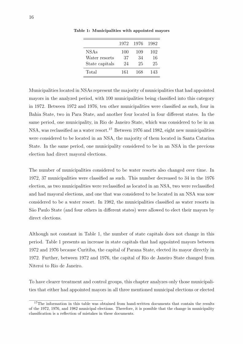
ipalities located in NSAs. Table 1 presents the number of municipalities classified into
each of these categories in 1972, 1976, and 1982, the three municipal elections for which
data are available.16
15The Demographic Census that was supposed to be carried out in 1990 was conducted in 1991 becauseof administrative issues.
16As previously mentioned, there was a municipal election in 1970 but data for this election areunavailable. Therefore, it is not possible to credibly identify which municipalities had appointed mayorsand why.
16
Table 1: Municipalities with appointed mayors
1972 1976 1982
NSAs 100 109 102Water resorts 37 34 16State capitals 24 25 25
Total 161 168 143
Municipalities located in NSAs represent the majority of municipalities that had appointed
mayors in the analyzed period, with 100 municipalities being classified into this category
in 1972. Between 1972 and 1976, ten other municipalities were classified as such, four in
Bahia State, two in Para State, and another four located in four different states. In the
same period, one municipality, in Rio de Janeiro State, which was considered to be in an
NSA, was reclassified as a water resort.17 Between 1976 and 1982, eight new municipalities
were considered to be located in an NSA, the majority of them located in Santa Catarina
State. In the same period, one municipality considered to be in an NSA in the previous
election had direct mayoral elections.
The number of municipalities considered to be water resorts also changed over time. In
1972, 37 municipalities were classified as such. This number decreased to 34 in the 1976
election, as two municipalities were reclassified as located in an NSA, two were reclassified
and had mayoral elections, and one that was considered to be located in an NSA was now
considered to be a water resort. In 1982, the municipalities classified as water resorts in
Sao Paulo State (and four others in different states) were allowed to elect their mayors by
direct elections.
Although not constant in Table 1, the number of state capitals does not change in this
period. Table 1 presents an increase in state capitals that had appointed mayors between
1972 and 1976 because Curitiba, the capital of Parana State, elected its mayor directly in
1972. Further, between 1972 and 1976, the capital of Rio de Janeiro State changed from
Niteroi to Rio de Janeiro.
To have clearer treatment and control groups, this chapter analyzes only those municipali-
ties that either had appointed mayors in all three mentioned municipal elections or elected
17The information in this table was obtained from hand-written documents that contain the resultsof the 1972, 1976, and 1982 municipal elections. Therefore, it is possible that the change in municipalityclassification is a reflection of mistakes in these documents.

17
mayors in the same three elections. Municipalities partially disenfranchised, that is, those
municipalities that had appointed mayors in only one or two of the referred elections are
therefore excluded from this analysis.
1.4 Empirical strategy
Identifying the effects of a change in political institutions such as having appointed mayors
during almost two decades on income distribution is not straightforward. Municipalities
that had appointed mayors were not randomly chosen; they were selected by the federal
government for specific reasons and therefore should be expected to be different from the
rest of the country in many dimensions. Table 2 presents the baseline characteristics of
Brazilian municipalities by different groups. The first column reports the characteristics of
all municipalities present in the 1970 Demographic Census. Columns (2) and (3) present
the characteristics of those municipalities that had appointed mayors in at least one of
the three elections between 1972 and 1982.
Table 2: Mean of the baseline (1970) socioeconomic characteristics
(1) (2) (3)
Allmunicipalities
Municipalitieswith appointed
mayors
Municipalitieswith appointedmayors (exceptstate capitals)
Inequality (Theil index) 35.12 40.19 38.19Share of pop. living in urban areas 32.16 43.99 36.17log(population) 9.39 10.25 9.81Population density (inhabitants/km2) 59.55 269.60 69.08Share of illiteracy 43.64 30.64 32.35Average years of schooling 1.39 2.27 2.01Income per capita (in minimum wages) 0.35 0.55 0.48Log(number of households) 7.69 8.54 8.10Life expectancy 51.26 53.25 53.61Share of pop. occupied 30.60 31.46 31.78Share of households with sanitation 4.97 10.18 8.95Share of households with piped water 14.57 26.73 22.72Share of households with electricity 24.00 37.24 31.72Share of pop. living in poverty 83.96 70.80 73.90
Number of municipalities 3951 172 146
Note: all the differences in columns (1) and (2) are significant at the 1% level. All the differences in columns (1) to (3) are significantat the 1% level, except Share of pop. living in urban areas (p-value=0.02) and Population density (p-value=0.70). The differencesin columns (2) and (3) are all significant at the 1% level, except Share of pop. occupied (p-value=0.04) and Share of householdswith sanitation (p-value=0.03).
As expected, column (2) shows that municipalities with appointed mayors are different
in numerous ways from the rest of the country. In particular, they are more urbanized,

18
more populated, wealthier, present better measures of schooling, and their citizens have
higher life expectancy. Therefore, simply comparing this group of municipalities with the
rest of the country would not be possible to assess the effect of having appointed mayors
on economic outcomes.
Since state capitals are likely to be different from the rest of the municipalities, column
(3) presents the characteristics of municipalities considered to be water resorts and those
located in NSAs. This shows that even excluding state capitals, municipalities that had
appointed mayors are very different from the rest of the country. Despite this notable
difference, however, it is reasonable to believe, based on what has been exposed in previous
sections, that these two groups of municipalities were chosen by the federal government to
have appointed mayors mainly because of their geographic characteristics (i.e. availability
of explorable water and proximity to borders). Figure 2 illustrates this fact by showing
the distribution of municipalities that had appointed mayors in at least one of the three
elections between 1972 and 1982. This figure shows that, especially for municipalities
located in NSAs, the selection was mainly driven by geographic characteristics, namely
being located on the border of the country. Although spread over the country, to be
considered a water resorts, a municipality had to meet a clear geographical requirement
(i.e having explorable water sources). Therefore, to minimize the concern with (political
and economic) selection, this chapter focuses its analysis on municipalities located in
NSAs and those considered to be water resorts. By doing so, the issue of the selection of
municipalities based on political and economic characteristics is substantially reduced. In
other words, by using this subset of municipalities that, arguably, were selected mainly
by their geographic characteristics, the main source of endogeneity becomes known and,
therefore, it is possible to develop a strategy to deal with it.

19
Figure 2: Municipalities with appointed mayors
Even by restricting the analysis to this subset of municipalities, it is still not possible to
simply compare municipalities with appointed mayors with the rest of the country to assess
the effect of this variation in political institutions. An alternative approach would be to
use geography as an instrument for disenfranchised municipalities (i.e. a dummy equal to
one if the municipality is in the border and/or a measure of the amounts of explorable
water in the municipality). The issue with this strategy, however, is the well documented
influence of geography on economic institutions and economic outcomes, thereby violating
the exclusion restriction.18
The empirical strategy employed in this chapter resembles that proposed by Keele, Titiu-
nik & Zubizarreta (2015) and used by Larreguy, Marshall & Snyder (2014), which can be
understood as a combination of geographic regression discontinuity (GRD) design with
matching techniques. By claiming that one of the main sources of selection is the munic-
ipality’s location, the strategy employed compares each municipality that had appointed
mayors with its most similar neighbor in terms of the Mahalanobis distance.
As for non-geographic regression discontinuity designs, causal effects are identified under
the assumption that potential outcomes are continuous in all other variables at the ge-
ographic discontinuity. Although it is not quite necessary, achieving balance across the
18For more on the debate about the relation between geography and economic institutions, see (Ace-moglu, Johnson & Robinson (2002)).

20
Figure 3: Municipalities with appointed mayors in the sample and neighbors used as thecontrol group
treatment and control groups is sufficient for continuity to hold Imbens & Lemieux (2008).
This motivates the decision to match over a set of covariates and select the most similar
non-treated municipalities in terms of the Mahalanobis distance.
More specifically, the construction of the sample entails the following procedure:
1. Identify potential matches. For each municipality with appointed mayors i, the set of
possible matches is restricted to the set of neighboring municipalities j that had mayors
elected directly in 1972, 1976, and 1982. This set of potential matching is denoted J(i).
2. Calculate the Mahalanobis distance D(Xi, Xj) =√
(Xi −Xj)′C−1(Xi −Xj) between
municipality i and each possible match j ∈ J(i) using the vector Xi of 14 covariates and
the full sample covariance matrix C.
3. Finally, for each treated municipality i, choose the control municipality taking the
nearest match in the set J(i).
Figure 3 illustrates the sample from the algorithm described above.
With the sample constructed, Equation 1.1 is estimated to assess the effect of appointed

21
mayors on the economic outcome of interest y in the municipality i:
yi = δ · yi,1970 + γ · appointedi + Xiβ + εi (1.1)
where appointed is a dummy variable that takes the value one for municipalities that
had appointed mayors in the analyzed period. Since this research is interested in the
changes in economic outcomes yi after a municipality had appointed mayors, the baseline
variable yi,1970 is also included in the regression. Although the results from balance checks
reported in Section 1.5.1 show that control and treatment groups are balanced in baseline
covariates constructed from the 1970 Demographic Census, the complete specification of
Equation 1.1 is estimated including the vector of covariates Xi as a control.
Equation 1.1 is run for the measures of inequality constructed from the 1980 and 1991
Demographic Censuses. Since the municipalities in the treatment group had appointed
mayors between the end of the 1960s and 1985, measuring the effects of appointed mayors
with minimum noise and avoiding confounding the effects with, for instance, possible het-
erogeneous effects of redemocratization among treatment and control groups would ideally
require estimating the effects on inequality (or any other possible outcomes of interest) im-
mediately after the treatment has ended (i.e. immediately after redemocratization in 1985
when all municipalities had direct mayoral elections). Unfortunately, this is not possible
since detailed socioeconomic data at the municipality level such as income distribution
measures were only collected in 1980 and 1991. Therefore, to provide evidence that the
results are indeed driven by having appointed mayors, this research tests for differences
in economic outcomes both in 1980 and in 1991. If appointed mayors affect the income
distribution, one should expect to see this effect increase over time. Moreover, it seems
unreasonable to believe that redemocratization would have different effects in municipali-
ties in the treatment and control groups, especially in terms of redistribution and in such
a short period. If anything, using measures of income inequality in 1991 introduces some
noise into the estimates.
One concern with the empirical strategy described is with confounding treatments, a
concern that naturally arises with strategies that rely on geography. By comparing mu-
nicipalities in specific locations with their neighbors, the effect identified may not only
be the effect of having appointed mayors per se but also be the effect of being in that
22
specific geographic area. In other words, proximity to a border or having large amounts of
explorable water may explain the findings presented in this chapter. To provide evidence
that this is not the case, a placebo exercise comparing non-treated neighbors as if they
were treated with their own non-treated neighbors is reported in Section 1.6.
To show that the main results are robust to the matching algorithm, in appendix A
the same exercises of the following section are reproduced; however, instead of using the
matching algorithm to identify each disenfranchised municipality’s closest neighbor, all
non-disenfranchised neighbors are used as counterfactual. In contrast to employing a
combination of geographic regression discontinuity design and matching, balance among
the control and treatment groups is not achieved. The main results, however, are qualita-
tively unchanged when municipality-level controls are included. The results are presented
in Tables 25–27. Figure 11 illustrates the sample constructed without the matching algo-
rithm.
1.5 Results
1.5.1 Balance check
This section begins by showing evidence that the empirical strategy described in the previ-
ous section results in a control group that is similar to the group of treated municipalities
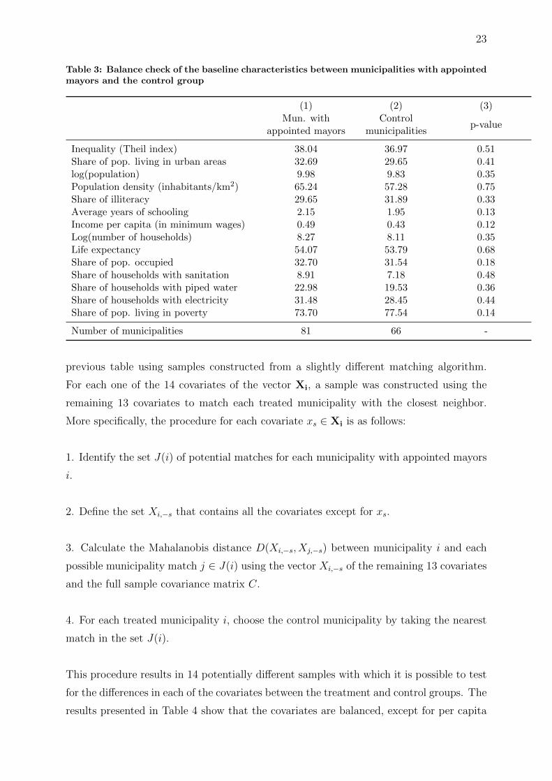
in a number of relevant predetermined characteristics. Table 3 reports the same statistics
presented in Table 2. In contrast to that table, however, it shows the mean characteristics
only for the subset of municipalities that had appointed mayors considered in the analysis
(i.e. state capitals and partially disenfranchised municipalities are not considered). The
comparison group also differs from that in Table 2 by including only the closest neighbor
of each disenfranchised municipality measured by the Mahalanobis distance.
As seen in columns (1) and (2), even when restricting the comparison to municipalities
with appointed mayors and their closest neighbors, the former present higher average
measures of urbanization, wealth, schooling, inequality, and population size. These dif-
ferences, however, are now not statistically significant at the usual levels.
To ensure that this balance in covariates is not simply a mechanical result of the match-
ing algorithm implemented, Table 4 reproduces the statistics and tests reported in the
23
Table 3: Balance check of the baseline characteristics between municipalities with appointedmayors and the control group
(1) (2) (3)Mun. with
appointed mayorsControl
municipalitiesp-value
Inequality (Theil index) 38.04 36.97 0.51Share of pop. living in urban areas 32.69 29.65 0.41log(population) 9.98 9.83 0.35Population density (inhabitants/km2) 65.24 57.28 0.75Share of illiteracy 29.65 31.89 0.33Average years of schooling 2.15 1.95 0.13Income per capita (in minimum wages) 0.49 0.43 0.12Log(number of households) 8.27 8.11 0.35Life expectancy 54.07 53.79 0.68Share of pop. occupied 32.70 31.54 0.18Share of households with sanitation 8.91 7.18 0.48Share of households with piped water 22.98 19.53 0.36Share of households with electricity 31.48 28.45 0.44Share of pop. living in poverty 73.70 77.54 0.14
Number of municipalities 81 66 -
previous table using samples constructed from a slightly different matching algorithm.
For each one of the 14 covariates of the vector Xi, a sample was constructed using the
remaining 13 covariates to match each treated municipality with the closest neighbor.
More specifically, the procedure for each covariate xs ∈ Xi is as follows:
1. Identify the set J(i) of potential matches for each municipality with appointed mayors
i.
2. Define the set Xi,−s that contains all the covariates except for xs.
3. Calculate the Mahalanobis distance D(Xi,−s, Xj,−s) between municipality i and each
possible municipality match j ∈ J(i) using the vector Xi,−s of the remaining 13 covariates
and the full sample covariance matrix C.
4. For each treated municipality i, choose the control municipality by taking the nearest
match in the set J(i).
This procedure results in 14 potentially different samples with which it is possible to test
for the differences in each of the covariates between the treatment and control groups. The
results presented in Table 4 show that the covariates are balanced, except for per capita

24
income, which is slightly higher in treated municipalities, with the difference significant
at the 10% level. The results not only show that the balance between the treatment and
control groups is not simply a mechanical result of the matching algorithm implemented
but also suggest that the treatment and control groups might be balanced in other relevant
(unobservable) characteristics.
Table 4: Balance check of the baseline characteristics between municipalities with appointedmayors and the control group (using N-1 covariates to match)
Mun. with appointed mayors Control municipalities p-valuemean obs mean obs(1) (2) (3) (4) (5)
Inequality (Theil index) 38.04 81 37.14 65 0.59Share of pop. living in urban areas 32.69 81 29.31 67 0.35log(population) 9.98 81 9.84 66 0.38Population density (inhabitants/km2) 65.24 81 93.20 66 0.52Share of illiteracy 29.65 81 31.80 63 0.37Average years of schooling 2.15 81 1.97 63 0.21Income per capita (in minimum wages) 0.49 81 0.42 64 0.06Log(number of households) 8.27 81 8.12 66 0.38Life expectancy 54.07 81 53.99 64 0.91Share of pop. occupied 32.70 81 31.54 65 0.18Share of households with sanitation 8.91 81 6.52 68 0.31Share of households with piped water 22.98 81 19.45 67 0.35Share of households with electricity 31.48 81 29.67 67 0.65Share of pop. living in poverty 73.70 81 77.60 67 0.13
Notes: each line presents the statistics of the test of the mean difference between the municipalities withappointed mayors and the control group. To construct the control group in this exercise, each municipalitywas matched to its most similar neighbor according to a set of N-1 covariates and the control group, with theomitted covariate being the variable tested for the difference in each line. Each line, therefore, may have adifferent control group.
1.5.2 Effects on income distribution
This section reports the main results of this chapter, the effect of having appointed mayors
for almost two decades on income distribution. Figure 4 illustrates the evolution of the
Theil index in municipalities that had appointed mayors during the dictatorship and in
neighboring control municipalities. In both groups of municipalities, inequality increased
substantially during the years of the military dictatorship, consistent with the discussion
in the previous sections.
Figure 4 also evidences that the increase in inequality is accentuated in disenfranchised
municipalities. Table 5 formalizes these results by showing the estimates of Equation 1.1.
The dependent variable appointed mayor is a dummy variable that takes the value one
if the municipality had appointed mayors in all three municipal elections between 1972

25
Figure 4: Theil index in municipalities with appointed and with elected mayors
and 1982 and zero if the municipality had mayors elected democratically. The dependent
variable is the Theil index measured in 1980 and 1991 and it is given by:
Theil index =1
N
N∑i=1
(xix· ln xi
x
)(1.2)
where xi is the income of each individual and x is the mean of x. If everyone has the same
income, then xi = x,∀i and the Theil index equals zero. On the contrary, if one person
has all the income, the index equals ln(N). The index is normalized to be in the interval
[0, 1].
Although the balance checks show that the control and treatment groups are balanced in
a number of dimensions (including inequality), the baseline Theil index is included in all
regressions to ensure that the variation in the index from one period to another is being
estimated. Columns (1) and (3) report the estimates of the effect of having appointed
mayors on the Theil index in 1980 and 1991, respectively, without including the baseline
controls. Columns (2) and (4) present the results of similar regressions but with the
inclusion of the vector of baseline controls Xi.
Table 5 shows that the difference in the increase in the Theil index between municipalities

26
Table 5: Effect on the Theil index
Dependent variable: Theil index in year t; covariates measured in t=1970
t=1980 t=1991(1) (2) (3) (4)
Appointed mayor 1.3974 1.3327 4.1105∗ 4.3194∗∗
(1.9138) (1.8442) (2.1142) (2.0024)Inequality (Theil index) 0.6540∗∗∗ 0.8013∗∗∗ 0.2671∗∗∗ 0.4151∗∗
(0.0888) (0.1507) (0.0955) (0.1608)Share of pop. living in urban areas 0.1521 0.1001
(0.1023) (0.0836)Log(population) -9.8572 22.9578
(15.9397) (16.4989)Population density -0.0076 -0.0035
(0.0083) (0.0069)Share of illiteracy -0.3938∗∗ 0.1045
(0.1700) (0.2320)Average years of schooling -6.0890∗ 0.0194
(3.1299) (3.9098)Income per capita (in minimum wages) -11.9974 -21.8445∗
(13.1049) (12.9617)Log(number of households) 10.8757 -21.3136
(15.8127) (16.7353)Life expectancy 0.3571 1.2109∗∗∗
(0.3612) (0.4240)Share of pop. occupied -2.4322 5.3908
(21.1955) (26.1852)Share of households with sanitation 0.2134∗∗ 0.1862∗
(0.0984) (0.0978)Share of households with piped water -0.2062∗∗ -0.1032
(0.0936) (0.0897)Share of households with electricity -0.2870∗∗ -0.0517
(0.1294) (0.1227)Share of pop. in poverty -0.3860 -0.1497
(0.2480) (0.2127)
Observations 147 147 147 147R-squared 0.24 0.41 0.07 0.28
Robust standard errors in parentheses: ∗ p < 0.10, ∗∗ p < 0.05, ∗∗∗ p < 0.01
27
with appointed mayors and the control group, although positive, is not significant in 1980.
The difference estimated in 1991, however, is not only positive but highly significant.
Further, both sets of results are robust to the inclusion of municipality–level controls.
Indeed, the point estimates do not change with the inclusion of these controls; they only
become more precise, providing further evidence the sample is fairly well balanced. The
results show that on average municipalities that had appointed mayors present a Theil
index around 4 points higher than their neighbors in 1991.19 In the same period, the
Theil index in Brazil went from 68 in 1970 to 78 in 1991. That is to say, having mayors
appointed by the dictatorship regime is associated with an increase in inequality similar
to 40% of the rise the country experienced during those two decades.
Although this research focuses on studying the presence of elite capture by measuring
income inequality, it is convenient to look at how other variables evolved during this
period in disenfranchised municipalities compared with their control neighbors. Tables 28
and 29 in appendix A show that the vast majority of the other socioeconomic variables did
not present significant differences between the treatment and control groups in 1980 and
1991. The only exceptions are the number of households and size of population, which
are larger in the treated municipalities, suggesting that not only inequality increased in
disenfranchised municipalities but they also become larger compared with the control
group.
The results presented thus far show that having appointed mayors is associated with
a significant increase in inequality. However, this increase in inequality cannot yet be
interpreted as the presence of elite capture. To shed light on the reasons behind the
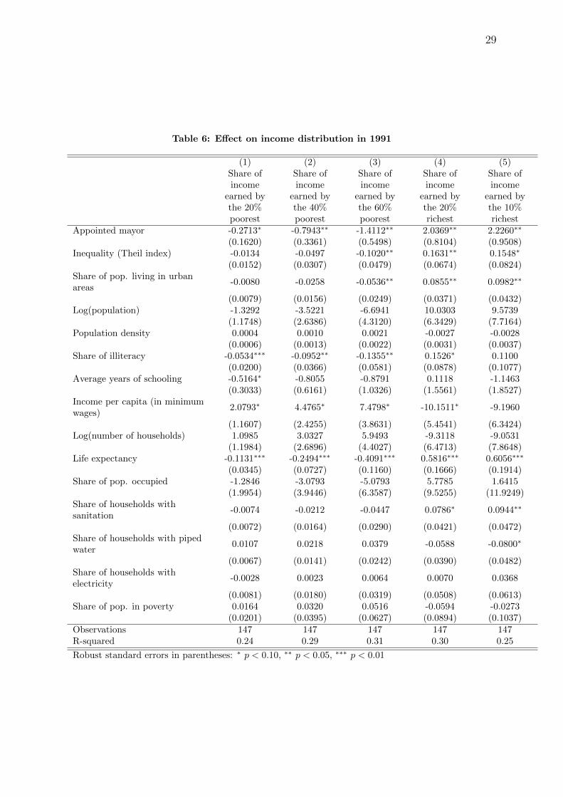
effects reported in the previous table, Table 6 presents results of the estimates of Equation
1.1 on the other measures of income distribution. The dependent variables used in these
regressions were constructed from the 1991 Demographic Census and show the share of the
municipality income earned by different quintiles of the population. In the first column,
the dependent variable is the share of income earned by the 20% poorest; in the second
column, the share earned by the 40% poorest; in the third column, the share earned by
the 60% poorest; in the fourth, the share earned by the 20% richest (or one minus the
share earned by the 80% poorest); and in the last column, the share earned by the 10%
richest (or one minus the share earned by the 90% poorest).
As discussed in Section 1.2, the understanding in the economic history literature is that the
19in 1970, as seen in Table 3, this difference was balanced between the two groups.

28
concentration of wealth in this period was mainly through a decrease in real wages, which
ended up punishing the lower classes of the population to a greater extent. Therefore, if
the increase in inequality in disenfranchised municipalities was simply a magnification of
the distributional effects that took place across the country, strong negative effects on the
share of the income earned by the poorest should be expected. However, according to the
estimates in Table 6, inequality increased in municipalities that had appointed mayors
more than it did in the control group mainly due to an increase in the share of income
earned by the richest. In other words, the situation of the poor in municipalities that had
appointed mayors and in neighboring municipalities changed similarly between 1970 and
1991. In the same period, the situation of the rich, on the contrary, improved dramatically
in municipalities that had appointed mayors compared with neighboring municipalities.
These results are consistent with a story of elite capture in these municipalities, especially
considering that this was a period of intense investment by the central government and
that, from the evidence documented in the political economy literature,20 these munici-
palities were more likely to receive (larger) federal investment because of their political
alignment. Ideally, this hypothesis could be better investigated by looking at expenditure
data. However, as such data are unavailable, this research relies on the latter findings and
on the results presented in Tables 28 and 29 in the appendix A, which imply that disen-
franchised municipalities increased more during this period and are, therefore, consistent
with the hypothesis that these municipalities received more investment.
20See Brollo & Nannicini (2012); Sole-Olle & Sorribas-Navarro (2008); Khemani (2007); Arulampalamet al. (2009); and Leao (2011).
29
Table 6: Effect on income distribution in 1991
(1) (2) (3) (4) (5)Share ofincome
earned bythe 20%poorest
Share ofincome
earned bythe 40%poorest
Share ofincome
earned bythe 60%poorest
Share ofincome
earned bythe 20%richest
Share ofincome
earned bythe 10%richest
Appointed mayor -0.2713∗ -0.7943∗∗ -1.4112∗∗ 2.0369∗∗ 2.2260∗∗
(0.1620) (0.3361) (0.5498) (0.8104) (0.9508)Inequality (Theil index) -0.0134 -0.0497 -0.1020∗∗ 0.1631∗∗ 0.1548∗
(0.0152) (0.0307) (0.0479) (0.0674) (0.0824)Share of pop. living in urbanareas
-0.0080 -0.0258 -0.0536∗∗ 0.0855∗∗ 0.0982∗∗
(0.0079) (0.0156) (0.0249) (0.0371) (0.0432)Log(population) -1.3292 -3.5221 -6.6941 10.0303 9.5739
(1.1748) (2.6386) (4.3120) (6.3429) (7.7164)Population density 0.0004 0.0010 0.0021 -0.0027 -0.0028
(0.0006) (0.0013) (0.0022) (0.0031) (0.0037)Share of illiteracy -0.0534∗∗∗ -0.0952∗∗ -0.1355∗∗ 0.1526∗ 0.1100
(0.0200) (0.0366) (0.0581) (0.0878) (0.1077)Average years of schooling -0.5164∗ -0.8055 -0.8791 0.1118 -1.1463
(0.3033) (0.6161) (1.0326) (1.5561) (1.8527)Income per capita (in minimumwages)
2.0793∗ 4.4765∗ 7.4798∗ -10.1511∗ -9.1960
(1.1607) (2.4255) (3.8631) (5.4541) (6.3424)Log(number of households) 1.0985 3.0327 5.9493 -9.3118 -9.0531
(1.1984) (2.6896) (4.4027) (6.4713) (7.8648)Life expectancy -0.1131∗∗∗ -0.2494∗∗∗ -0.4091∗∗∗ 0.5816∗∗∗ 0.6056∗∗∗
(0.0345) (0.0727) (0.1160) (0.1666) (0.1914)Share of pop. occupied -1.2846 -3.0793 -5.0793 5.7785 1.6415
(1.9954) (3.9446) (6.3587) (9.5255) (11.9249)Share of households withsanitation
-0.0074 -0.0212 -0.0447 0.0786∗ 0.0944∗∗
(0.0072) (0.0164) (0.0290) (0.0421) (0.0472)Share of households with pipedwater
0.0107 0.0218 0.0379 -0.0588 -0.0800∗
(0.0067) (0.0141) (0.0242) (0.0390) (0.0482)Share of households withelectricity
-0.0028 0.0023 0.0064 0.0070 0.0368
(0.0081) (0.0180) (0.0319) (0.0508) (0.0613)Share of pop. in poverty 0.0164 0.0320 0.0516 -0.0594 -0.0273
(0.0201) (0.0395) (0.0627) (0.0894) (0.1037)
Observations 147 147 147 147 147R-squared 0.24 0.29 0.31 0.30 0.25
Robust standard errors in parentheses: ∗ p < 0.10, ∗∗ p < 0.05, ∗∗∗ p < 0.01

30
1.6 Placebo exercise
Since part of the empirical strategy employed in this chapter relies on geography, one
possible concern is that the effects documented in the previous sections are not (entirely)
related to having appointed mayors but are (also) a result of being in a specific geograph-
ical area. This section reports the results of a placebo exercise conducted to reject this
hypothesis. The exercise considers as treated all non-disenfranchised neighbors of disen-
franchised municipalities (considered in the previous analysis) and compares them with
their closest non-disenfranchised neighbors, using a matching algorithm similar to that
described in Section 1.4.21
If the effect documented in the previous section is (partially) driven by being close to
the border of the country – in the case of municipalities located in NSAs – or in an area
with large amounts of explorable water – in the case of municipalities considered to be
water resorts – similar results should be expected when estimating equation 1.1 in this
particular sample. This would not be the case in the unlikely hypothesis that the effect
associated with being in a specific geographic area changes discretely. In such a scenario,
it would be impossible to disentangle both effects with the strategy employed.
Figure 5 illustrates the placebo exercise. Non-disenfranchised neighbors of disenfranchised
municipalities are considered to be treated in this case. A similar matching algorithm is
then carried out with their non-disenfranchised neighbors to identify the closest neighbor
to be used as the control.
To provide evidence that the strategy employed is able to construct a placebo group
that is similar to its respective control group, Table 7 reports the results of a balance
check exercise, similar to that in Table 3 for the main sample. The results show that
the only variable that is not balanced across the placebo and control group is the share
of population living in poverty. All the other covariates have a non-significant difference
between both groups.
Tables 8 and 9 reproduce the main regression of the chapter using the placebo sample de-
scribed above. There is no significant effect in the Theil index measured in 1980 and 1991,
21A more natural alternative would be to consider as treated only the closest neighbor of each treatedmunicipality. This alternative, however, would result in a smaller sample, which could lead to non-significant results due to low power.

31
Figure 5: Placebo exercise: Treated municipalities and neighbors used as the control group
Table 7: Placebo: balance check of the baseline characteristics between treated municipal-ities and the control group
(1) (2) (3)Placebo Control p-value
Inequality (Theil index) 36.69 36.92 0.85Share of pop. living in urban areas 31.49 28.67 0.15log(population) 9.49 9.47 0.86
Population density (inhabitants/km2) 47.62 63.67 0.51
Share of illiteracy 37.08 37.16 0.96Average years of schooling 1.67 1.65 0.80Income per capita (in minimum wages) 0.43 0.39 0.10Log(number of households) 7.79 7.78 0.90Life expectancy 52.33 52.43 0.83Share of pop. occupied 31.04 30.92 0.78Share of households with sanitation 7.46 6.68 0.61Share of households with piped water 19.92 17.81 0.35Share of households with electricity 28.65 27.11 0.55Share of pop. living in poverty 77.87 80.73 0.10
Number of municipalities 195 133 -

32
nor in the share of income earned by different percentiles of the population, strengthen-
ing the hypothesis that the effect is unrelated to geographic characteristics and rather
associated with the regime appointing mayors for almost two decades.
Table 8: Placebo: effect on the Theil index
Dependent variable: Theil index in year t; covariates measured in t=1970
t=1980 t=1991(1) (2) (3) (4)
Placebo -1.4369 -1.7202 0.5651 0.4807(1.4630) (1.3381) (1.4391) (1.3907)
Inequality (Theil index) 0.4994∗∗∗ 0.4392∗∗∗ 0.2384∗∗∗ 0.1896∗∗
(0.0698) (0.0831) (0.0694) (0.0875)Share of pop. living in urban areas 0.0680 0.0172
(0.0622) (0.0658)Log(population) -1.8002 23.2242∗∗
(9.9337) (10.3205)Population density -0.0098∗∗∗ -0.0084∗∗∗
(0.0035) (0.0027)Share of illiteracy -0.2386 0.2293∗∗
(0.1521) (0.1104)Average years of schooling 1.7761 9.8316∗∗∗
(2.5963) (2.3586)Income per capita (in minimum wages) -7.0393 3.9113
(12.3962) (13.3618)Log(number of households) 3.0282 -21.9814∗∗
(9.9530) (10.2413)Life expectancy 0.2897 0.2669
(0.2352) (0.2341)Share of pop. occupied -8.7884 -23.2466
(28.2077) (20.1244)Share of households with sanitation -0.0275 -0.0841
(0.0847) (0.0944)Share of households with piped water -0.0282 -0.0685
(0.0733) (0.0793)Share of households with electricity -0.2392∗∗∗ -0.1128
(0.0818) (0.0789)Share of pop. in poverty -0.2157 0.0584
(0.1796) (0.1843)
Observations 328 328 328 328R-squared 0.17 0.32 0.04 0.19
Robust standard errors in parentheses: ∗ p < 0.10, ∗∗ p < 0.05, ∗∗∗ p < 0.01

33
Table 9: Placebo: effect on income distribution in 1991
(1) (2) (3) (4) (5)Share ofincome
earned bythe 20%poorest
Share ofincome
earned bythe 40%poorest
Share ofincome
earned bythe 60%poorest
Share ofincome
earned bythe 20%richest
Share ofincome
earned bythe 10%richest
Placebo -0.0377 -0.0638 -0.0738 0.0751 -0.0040(0.0959) (0.2277) (0.3991) (0.6089) (0.7196)
Inequality (Theil index) -0.0037 -0.0197 -0.0417 0.0776∗ 0.0918∗∗
(0.0063) (0.0148) (0.0258) (0.0396) (0.0459)Share of pop. living in urban areas -0.0032 -0.0052 -0.0125 0.0162 0.0182
(0.0047) (0.0114) (0.0200) (0.0306) (0.0352)Log(population) -2.4119∗∗∗ -4.5505∗∗ -7.1881∗∗ 8.8067∗ 9.0558∗
(0.8265) (1.9174) (3.2623) (4.7612) (5.3916)Population density 0.0006∗∗∗ 0.0015∗∗∗ 0.0028∗∗∗ -0.0040∗∗∗ -0.0043∗∗∗
(0.0001) (0.0004) (0.0008) (0.0013) (0.0015)Share of illiteracy -0.0220∗∗ -0.0496∗∗ -0.0902∗∗∗ 0.1186∗∗ 0.1191∗∗
(0.0092) (0.0198) (0.0337) (0.0513) (0.0599)Average years of schooling -0.8197∗∗∗ -1.9223∗∗∗ -3.2204∗∗∗ 3.9467∗∗∗ 3.6869∗∗∗
(0.1508) (0.3686) (0.6861) (1.0968) (1.2741)Income per capita (in minimumwages)
-0.2753 -0.9571 -2.6795 3.6392 3.4118
(1.0091) (2.2804) (4.0082) (6.2840) (7.1242)Log(number of households) 2.2352∗∗∗ 4.1479∗∗ 6.5570∗∗ -8.0269∗ -8.4462
(0.8256) (1.9095) (3.2447) (4.7380) (5.3655)Life expectancy -0.0205 -0.0492 -0.0886 0.1182 0.0818
(0.0186) (0.0413) (0.0698) (0.1050) (0.1223)Share of pop. occupied 1.2378 3.7409 6.7186 -12.7181 -16.2033
(1.4382) (3.3880) (5.9603) (9.0014) (10.1398)Share of households with sanitation 0.0063 0.0143 0.0209 -0.0235 -0.0281
(0.0064) (0.0148) (0.0262) (0.0413) (0.0492)Share of households with pipedwater
0.0133∗∗∗ 0.0192 0.0237 -0.0146 -0.0027
(0.0050) (0.0126) (0.0233) (0.0371) (0.0436)Share of households with electricity 0.0007 0.0177 0.0417∗ -0.0631∗ -0.0604
(0.0056) (0.0130) (0.0231) (0.0368) (0.0438)Share of pop. in poverty -0.0041 -0.0129 -0.0324 0.0453 0.0465
(0.0136) (0.0316) (0.0553) (0.0851) (0.0956)
Observations 328 328 328 328 328R-squared 0.21 0.22 0.21 0.17 0.13
Robust standard errors in parentheses: ∗ p < 0.10, ∗∗ p < 0.05, ∗∗∗ p < 0.01

34
1.7 Conclusions
This chapter contributes to the political economy literature by studying the existence of
capture at local levels of government, a question still underexplored in the body of em-
pirical research, in the context of the Brazilian dictatorship. This is done by comparing
measures of inequality between municipalities that had appointed mayors during the dic-
tatorship with a set of municipalities where mayors were elected directly. The Brazilian
dictatorship is an interesting context within which to study such a phenomenon for two
reasons. First, it provides this unusual variation in political institutions at the local level.
Second, this period was characterized by a large number of ambitious central govern-
ment projects, implying a large amount of resources spent, which allows to investigate the
presence of practices related to capture.
To overcome the clear issue of the selection of disenfranchised municipalities, this chapter
combines a GRD design with matching techniques, relying on the hypothesis that the
main source of selection is related to the geographic characteristics of the municipalities.
Evidence is provided that the strategy employed results in a control group that is similar
to the group of treated municipalities in a number of relevant predetermined (observable)
characteristics.
The main findings are consistent with the hypothesis of elite capture at the local level,
since they indicate an increase not only in income inequality in municipalities that had
mayors appointed by the regime but also in the share of income earned by the richest.
Nonetheless, the results are also consistent with other stories (i.e: stronger presence of mil-
itary officials in municipalities that had appointed mayors, different incentives/preferences
between elected and appointed mayors, non-continuous effects of geography).

35
2 MEDIA CAPTURE IN NON-DEMOCRATIC REGIMES: EVIDENCEFROM THE BRAZILIAN DICTATORSHIP
2.1 Introduction
The question of how and to what extent media can affect voting behavior and political
and economic outcomes has been extensively discussed in both the economics and political
science literature 22 An interesting related topic that has been studied in recent years is
the extent to which media vehicles are prone to political capture. Theoretical evidence
suggests that media capture depends on institutional characteristics and media market
characteristics.23
This chapter investigates this particular issue in the context of the Brazilian dictatorship
(1964–1985). This context is interesting for two reasons. First, in non-democratic regimes,
media vehicles are expected to be more prone to political capture. In fact, one theoretical
result documented by Besley & Prat (2006) and Prat & Stromberg (2011) is that when
the transaction costs between the government and media industry are lower, industry is
more likely to be captured in equilibrium. Second, the period analyzed in this chapter is
one characterized by low competition and large expansion of the television market.24 A
second important theoretical result directly linked to this point and documented by the
same authors is that media pluralism could provide protection against capture.
Capture is only an intermediate phenomenon and one that is difficult to measure directly.
We are more interested in the effect of capture on key political outcomes Prat & Strom-
berg (2011). Therefore, to address this issue, this chapter investigates the effects of Rede
Globo (hereafter, Globo), the primary Brazilian television station, on electoral outcomes
of mayoral elections during the Brazilian dictatorship, mainly on the share of votes ob-
tained by Alianca Renovadora Nacional (hereafter, ARENA), the ruling party during the
dictatorship. To identify such effects, this chapter exploits the timing of Globo’s entry
into different municipalities. The main empirical challenge for identifying if the pres-
ence of Globo in a municipality affects electoral outcomes is the possibility that its entry
is correlated with political preferences at the municipality level. The results indicates
that, conditional on a set of municipality–level controls and on municipality and year
22See Besley & Burgess (2002), Dyck & Zingales (2002) and Hamilton (2004).23See Besley & Prat (2006) and Prat & Stromberg (2011).24According to Straubhaar (1989), Globo had roughly 70% of the audience by the end of the 1980s.

36
fixed-effects, there is no evidence of a politically driven entry of Globo.
The main effects documented in this chapter show that Globo has an average negative
effect on ARENA’s vote-share in the three mayoral elections between 1972 and 1982.
In principle, this is not consistent with the hypothesis of media capture. Evaluating the
results more deeply, however, shows that during the first years of the military dictatorship,
Globo has a positive effect on ARENA’s vote-share. In the latter years, however, the effect
becomes negative and, on average, overlaps the positive result. These results are consistent
with the theoretical result documented by Prat & Stromberg (2011), according to which
the presence of a news-related profit motive makes it more difficult for media vehicles to
be captured. Anecdotal evidence discussed latter in this chapter suggests that this is the
case. Straubhaar (1989) and Porto (2008) suggest that as a response to the new context of
political and economic crisis, Globo assumed a critical role in the last years of the regime,
ignoring censorship and incorporating problems and demands of the social reality in their
shows.
In order to better understand this sudden break in Globo’s effect, the content of Brazilian
soap operas, known as novelas, were coded and used in the analysis presented here. The
main results show that exposure to novelas with politically related content has a negative
effect on ARENA’s vote-share.
The literature focusing on media capture is scarce. Probably the most convincing evi-
dence of the existence of media capture was provided by McMillan & Zoido (2004). These
authors use a data set to reconstruct a complex system of bribes created during Alberto
Fujimori’s presidency in Peru from 1990 to 2000. To keep democratic forces at bay,
Fujimori needed to buy acquiescence from three classes: legislators, judges, and media
vehicles. Therefore, their study offers a unique perspective on the process of subverting
democracy. In particular, it investigates which of these three classes posed the strongest
resistance to Fujimori. The study’s main finding is that bribing the media is much more
expensive than bribing individuals. According to the paper, Fujimori spent ten times more
on bribes to television channels than bribes to politicians to secure a majority in Congress
or for guaranteeing a friendly judiciary. Additional evidence on media capture was pro-
vided by Tella & Franceschelli (2009), who analyzed each of the four major newspapers
in Argentina between 1998 and 2007. The focus was on how much first-page coverage
is devoted to corruption scandals and how much money each newspaper receives from
government-related advertising. The authors found a strong negative correlation between
37
these two variables.
A broader and more closely related literature documents the relationship between media
freedom/media competition and economic and electoral outcomes. Using a panel data
from India, Besley & Burgess (2002) show that state governments are more responsive to
decreases in food production and crop flood damage where newspaper circulation is higher
and electoral accountability is greater. Stromberg (2004) shows a positive correlation
between radio listeners and relief funds from the New Deal. In a cross-country study
using data on media ownership in 97 countries, Djankov et al. (2001) documents that
state ownership of the media is related to less press freedom, fewer political and economic
rights, and inferior social outcomes in the areas of education and health. Gentzkow,
Glaeser & Goldin (2006) use historical data to study the long-term evolution of media
independence and associate the reduction of corruption in the United States between 1870
and 1920 to changes in the American newspaper industry occurring in the same period.
This chapter also refers to the empirical literature on media bias (DellaVigna & Kaplan
(2006);Herman & Chomsky (2010); Groseclose & Milyo (2005) and Puglisi (2011)) and
the broader literature discussing the effects of media on political outcomes (Gentzkow
(2006); Gerber & Green (2000); Gerber, Karlan & Bergan (2006); George & Waldfogel
(2002) and Prior (2007)).
The remaining chapter sections are organized as follows. Section 2.2 discusses how mayoral
elections were organized in Brazil during the dictatorship, the relationship between Globo
and the dictatorship and the relevance of novelas. Section 2.3 describes the datasets on
election outcomes, Globo’s coverage, and novela content used in this chapter. Section 2.4
details the empirical strategy. Section 2.5 presents the main results. Section 2.6 concludes.
2.2 Institutional Background
2.2.1 Elections during the Brazilian dictatorship
The Brazilian military dictatorship began in March 1964 when President Joao Goulart
was overthrown by a coup d’etat led by the Armed Forces. It lasted for more than 20 years
and officially ended in 1985, when Jose Sarney, elected by indirect elections, took office as
president. Besides a set of measures that characterize all dictatorships, including political
38
violence, persecution of the opposition, and legislative casuistry, the Brazilian military
dictatorship had a unique political system compared to other dictatorships. For example,
when the head of government is in power without interruption, parties are forbidden to
work, Congress is closed, and the elections are suspended. During most years of the
military government, military-presidents and state governors were chosen by the National
Congress and State Legislative Houses, respectively. Moreover, legislative representatives
such as senators, congressmen, state legislators, and city councilors continued to be chosen
by direct vote during the entire regime. In contrast, mayors were elected by direct vote
during all years of the regime in most municipalities.25
The partisan system in Brazil during the period analyzed in this chapter should also
be highlighted. The multi–party system created in 1946 was abolished in 1965 by In-
stitutional Act Number 2, which created a two–party system, with ARENA (Alianca
Renovadora Nacional), the ruling party, and MDB (Movimento Democratico Brasileiro)
playing the role of the opposition. Until the end of the 1970s, these two political parties
were the only ones officially registered and able to run for election. In 1979, however, law
number 6767 extinguished both parties and created a multi-party system.26 Among other
things, the law instituted in 1979 stated that political parties should have the word party
– partido in Portuguese – in their names. Therefore, MDB became PMDB (Partido do
Movimento Democratico Brasileiro). ARENA, in turn, was recreated by its leaders as the
Partido Democratico Social (PDS). Three other parties that obtained registration to run
in the 1982 elections, Partido Trabalhista Brasileiro, Partido Democratico Trabalhista and
Partido dos Trabalhadores, comprised politicians whose political rights had been revoked
during the early years of the dictatorship in addition to other politicians returning from
exile.
Table 10 shows the elections during the military dictatorship, including four rounds of
mayoral elections. The first round was not simultaneous in all states and occurred between
1965 and 1970. The other three rounds occurred in 1972, 1976, and 1982 in all states of
the country simultaneously; these are the elections analyzed in this chapter.
Although the analysis focuses on mayoral elections, the general scenario of elections are es-
25State capitals, municipalities considered to be water resorts and municipalities located in nationalsecurity areas had mayors appointed by the state governors. This chapter is not concerned with thereasons behind the government’s determination that these municipalities would have mayors appointed.This issue only affects the external validity of this study’s results.
26Available at <http://www.planalto.gov.br/ccivil 03/leis/1970-1979/L6767.htm>.

39
sential to understand. Until 1973, the Brazilian economy underwent high rates of growth27
and as a result, ARENA fared well in both local and national elections Nicolau (2012).
After 1973, with the onset of the oil crisis, economic growth slowed. Consequently, the
opposition party started to grow and faced its first electoral win in the 1974 election. In
response to this shifting political scenario, President Ernesto Geisel established a project
of political openness that intended to be “slow, gradual and safe”, in his own words (Porto
(2008)). The creation of a multi-party system and the gubernatorial elections in 1982
listed in Table 10 can be understood as reflecting this process.
Table 10: Direct elections during the Brazilian military dictatorship
FederalDeputies and
SenatorsGovernor State Deputy
Mayors andCity Council
1965 October 3rd
1966 November 15th November 15th November 15th
1968 November 15th
1969 November 30th
1970 November 15th November 15th November 15th
1972 November 15th
1974 November 15th November 15th
1976November 15th
/ December20th
1978 November 15th November 15th
1982 November 15th November 15th November 15th November 15th
Source: http://www.tse.jus.br/eleicoes/cronologia-das-eleicoes
27This period, known as the “Brazilian miracle”,was discussed in the previous chapter.
40
2.2.2 Rede Globo and the military regime
It is not possible to state that Globo’s establishment in 1965 marks the beginning of the
television history in Brazil, but it does mark the beginning of the history of mass media
there. The story of television in Brazil began in 1950 with TV Tupi, but only after the
middle of the 1960s, a period coinciding with the foundation of Globo,28 did television
become a popular media instrument in Brazil. This is due to two main factors. The first
factor involved Globo’s strategy of aiming at the more general public by broadcasting
popular shows (Almeida (1971)). Second, credit policies were implemented during the
military regime, which were meant to provide incentives to buy durable goods such as
televisions, the sales of which greatly increased during this period.29
Both Globo’s geographical expansion and their audience increased rapidly over the decades.
In 1970, only five years after its official establishment, around 200 municipalities were cov-
ered by Rede Globo. In 1980, this figure had increased to more than 2000 municipalities,
more than half of all municipalities nationwide at that time. In addition, according to
Straubhaar (1989), Globo had roughly 70% of the Brazilian audience by the end of the
1980s.
For the purpose of this chapter’s identification strategy, understanding how the expansion
of Rede Globo occurred is essential. Despite the conclusions of some studies that the
concessions of televisions networks followed clientelistic, political and ideological criteria
(Lima (2001)), results presented latter in this chapter show that this argument is not
supported by the data. In fact, according to results documented here, the decision of
Globo to enter a municipality can be explained more by measures of income and by the
share of households with a television in the municipality.
Nonetheless, the role played by Globo during the military government cannot be ignored.
In fact, this topic has been studied by many authors from many disciplines.30 The general
understanding is that Globo was a main supporter of the coup d’etat and that it was
used by the regime as a key vehicle for cultural, political, and economic integration of the
28Rede Globo the television company was founded in 1965. The company’s newspaper O Globo existedsince 1925.
29The sales of black-and-white televisions in Brazil grew 241% between 1867 and 1979, whereas thoseof color televisions grew 1479% between 1972 and 1979 (Mattos (1982)).
30For a detailed discussion on the relationship between television and the dictatorship regime, seeStraubhaar (1989).
41
country (Miguel (2001)). In an editorial published in September 2013, Rede Globo itself
came to recognize many years after the end of the military regime the support that its
newspaper, O Globo, provided for the 1964 coup:
Rede Globo, in fact, at the time, supported the military intervention. (...)
Back then, the military intervention was justified for fear of another coup by
President Joao Goulart, with broad support from unions and some segments
the Armed Forces. (...) Through the light of the history, however, there is no
reason not to recognize today, explicitly, that the support was a mistake as
were other editorial decisions of the period.31
The role played by Globo during the dictatorship, however, changed over time. If in the
beginning of the regime, Globo clearly supported the central government, the scenario
changed in later years. According to Straubhaar (1989), in the last years of the regime,
Globo assumed a critical role by ignoring censorship warnings and airing live coverage of
demonstrations during days and evenings as well as in formal newscasts. In April 1984,
for example, Globo covered a major rally for direct elections in Rio de Janeiro for one
hour spread across the day, including during the prime-time novelas and newscasts. Porto
(2008) suggests that the relationship between Globo and the dictatorship changed, with
Globo incorporating problems and social demands in their shows, as a response to the
new context of political and economic crisis.
2.2.3 The importance of Globo Novelas
In order to understand the results presented here, the importance of Globo Novelas should
be emphasized. Faria & Potter (1999) stress the role played by television for the function
and presentation of contemporary Brazilian society and in the process of diffusing and
institutionalizing new behavioral patterns nationwide. In fact, this has been documented
empirically by Ferrara, Chong & Duryea (2012) and by Chong & Ferrara (2009) studying
the effects of novelas on fertility and divorce rates, respectively.
One crucial reason for television’s influence in Brazil is the strength of the country’s oral
tradition. This is especially relevant in the period discussed in this paper, in which the
31Source: <http://oglobo.globo.com/brasil/apoio-editorial-ao-golpe-de-64-foi-um-erro-9771604>

42
illiteracy rate is very elevated.32 Another factor contributing to novelas’ influence on
Brazilian life is that the context and issues they commonly address always relate to the
daily lives of the Brazilian population. Moreover, novelas use colloquial language that
renders the shows accessible to more viewers and thus results in their enormous success
(Ferrara, Chong & Duryea (2012)).
The story of Globo’s novelas during the dictatorship can be understood in two distin-
guished moments that coincided with the process of political opening and the shift in
Globo’s support to the military dictatorship. The first phase between 1964 and 1973 was
strongly shaped by the military dictatorship. The novelas had to constrain their criti-
cisms to political and economic issues, maintain conventional social behaviors and morals,
and most importantly, they had to create and reinforce a positive image of the regime
(Straubhaar (1988)). After 1973, however, as previously mentioned, the relationship be-
tween Globo and the dictatorship changed, and this had a reflect on the content of the
novelas, with problems and demands of social reality being incorporated into them.
2.3 Data
2.3.1 Municipal elections
The main dependent variables used in this chapter were constructed from historical files
of the Federal Electoral Authority, the Tribunal Regional Eleitoral (TSE). They contain
outcomes of the 1972, 1976, and 1982 mayoral elections. As previously mentioned, not
all municipalities had mayoral elections during the military dictatorship. This research is
not concerned with the issue of selection in the choice of these municipalities, as this only
affects the external validity of the results in the sense that they cannot be extrapolated to
the entire country. In other words, the results are valid only for the subset of municipalities
hosting mayoral elections between 1972 and 1982. These were typically smaller and more
rural than the municipalities with appointed mayors, especially state capitals.
The variables obtained from the TSE files were ARENA’s vote-share, voter turnout, the
share of blanks and null votes, and MDB’s vote-share. This analysis is focused on the first
three variables, especially the vote-share of the ruling party, ARENA. Figure 6 shows the
32In 1970, the adult illiteracy rate was 32.97%. Despite programs of the central government to reduceadult illiteracy during the years of the regime, this rate had decreased to only 19.40% in 1990.

43
Figure 6: Electoral outcomes in 1972, 1976 and 1982 mayoral elections
average of the main variables of interest over time.
Voter turnout increases over time, from around 78.5% in 1972 to more than 82% in 1982.
In fact, this is a period with huge increases in both voter turnout and voter registration.
Nicolau (2012) documents that between 1966 and 1982, the proportion of citizens reg-
istered to vote increased from 39% to 73%. According to him, two factors might have
played a significant role on this phenomenon. First, the Electoral Code approved in 1965
predicted a series of sanctions for voters who do not vote. Before approval of this code, the
voter who failed to vote had only to pay a fine, but after its approval, voters could experi-
ence a series of difficulties such when they applied for a job in a state-managed company,
had a passport issued, or obtained a loan from public banks, to name a few.33 Second,
with the increase of children in schools in the 1940s and 1950s, the number of young liter-
ate people increased significantly after 1960: the share of illiterate adults decreased from
40% in 1970 to 26% in 1980, according to demographic censuses from that period. Besides
these demographic and educational changes, Limongi, Cheidub & Figueiredo (2015) also
stress the role of urbanization in decreasing the cost of registering and the effort invested
by MDB in convincing voters to participate in local elections.
ARENA’s vote-share decreases over time. Between 1972 and 1976, the share of votes
33Available at <http://www.tse.jus.br/legislacao/codigo-eleitoral/codigo-eleitoral-1/sumarios/sumario-codigo-eleitoral-lei-nb0-4.737-de-15-de-julho-de-1965>
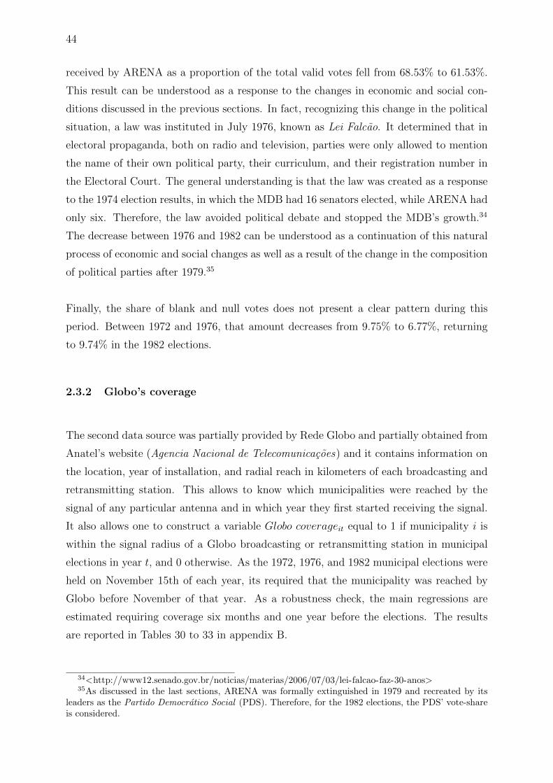
44
received by ARENA as a proportion of the total valid votes fell from 68.53% to 61.53%.
This result can be understood as a response to the changes in economic and social con-
ditions discussed in the previous sections. In fact, recognizing this change in the political
situation, a law was instituted in July 1976, known as Lei Falcao. It determined that in
electoral propaganda, both on radio and television, parties were only allowed to mention
the name of their own political party, their curriculum, and their registration number in
the Electoral Court. The general understanding is that the law was created as a response
to the 1974 election results, in which the MDB had 16 senators elected, while ARENA had
only six. Therefore, the law avoided political debate and stopped the MDB’s growth.34
The decrease between 1976 and 1982 can be understood as a continuation of this natural
process of economic and social changes as well as a result of the change in the composition
of political parties after 1979.35
Finally, the share of blank and null votes does not present a clear pattern during this
period. Between 1972 and 1976, that amount decreases from 9.75% to 6.77%, returning
to 9.74% in the 1982 elections.
2.3.2 Globo’s coverage
The second data source was partially provided by Rede Globo and partially obtained from
Anatel’s website (Agencia Nacional de Telecomunicacoes) and it contains information on
the location, year of installation, and radial reach in kilometers of each broadcasting and
retransmitting station. This allows to know which municipalities were reached by the
signal of any particular antenna and in which year they first started receiving the signal.
It also allows one to construct a variable Globo coverageit equal to 1 if municipality i is
within the signal radius of a Globo broadcasting or retransmitting station in municipal
elections in year t, and 0 otherwise. As the 1972, 1976, and 1982 municipal elections were
held on November 15th of each year, its required that the municipality was reached by
Globo before November of that year. As a robustness check, the main regressions are
estimated requiring coverage six months and one year before the elections. The results
are reported in Tables 30 to 33 in appendix B.
34<http://www12.senado.gov.br/noticias/materias/2006/07/03/lei-falcao-faz-30-anos>35As discussed in the last sections, ARENA was formally extinguished in 1979 and recreated by its
leaders as the Partido Democratico Social (PDS). Therefore, for the 1982 elections, the PDS’ vote-shareis considered.
45
Figure 7: Increase of Rede Globo coverage over time
Figure 7 shows the increase over time in the number of municipalities reached by the
Globo signal. In 1970, around 200 municipalities were receiving the Globo signal. By
the end of 1976 and 1982, this number increased to over 1000 and 3000 municipalities,
respectively.
Figure 8 shows the geographic expansion of the network between 1965 and 1982. Darker
colors correspond to an earlier exposure to the signal. This figure suggests that the entry
of Globo into different areas was not random, but it had a clear pattern: Globo reached
the most developed parts of Brazil first, specifically in the southeast and the capitals of
the northeast, which is potentially a concern for identifying the causal relation between
Globo and electoral outcomes. Results of exercises presented in Section 2.5.1, however,
show that after controlling for time-varying controls and municipality and year fixed-
effects, no evidence of selection on unobservable characteristics correlated with electoral
outcomes is found, especially with ARENA’s vote-share, which represents the primary
outcome of interest in this chapter.

46
Figure 8: Geographical distribution of Rede Globo’s coverage over time
2.3.3 Novela content analysis
To help understand the effect of Globo on electoral outcomes, the content of each novela
broadcast by Rede Globo since the start of its operations and 1982 were coded. Based
on a summary of plots obtained in the official website http://memoriaglobo.globo.com/,
a dataset with a series of variables describing the content of each novela was constructed.
Table 11 presents the description of each variable created from the summaries.
Table 12 presents the main results of the coding and summarizes the main characteristics
of novelas aired in this period. Column (1) presents the share of novelas with a specific
content aired between the beginning of Globo’s operation and November 1972, the month
of the first mayoral election studied here. Column (2) shows the same figures but for
novelas aired between November 1972 and November 1976. Finally, column (3) presents
novelas aired between November 1976 and November 1982.
Consistent with what was discussed in previous sections, Table 12 shows that the content
of novelas change over time. The change in the contents, however, was not abrupt. As
observed by Straubhaar (1989), this process was slowed by both official and internal cen-
sorship. The figures in Table 12 illustrate this fact. Comparing column (1) to column (2),

47
Table 11: Novela content coding
Variable Description Coding options
Political Issues Discussion of political issues 0 = does not discuss1 = discuss in the main plot2 = discuss in one of the secondary plots
Nature of Political Issue Nature of the political issues discussed 0 = does not discuss1 = Corruption2 = Elections3 = Allocation of public resources4 = Demand for democracy5 = Other/Not clear in the summary
Political CharacterPresence of a character that makes oppositionto the ruling party/to a powerful group
0 = does exist a character that makes opposi-tion to the ruling party/to a powerful group1 = one of the main characters makes opposi-tion to the ruling party/to a powerful group2 = one of the secondary characters makesopposition to the ruling party/to a powerfulgroup
HistoricalMain plot of the Soap Opera is not contempo-raneous
0 = plot is contemporaneous
1 = plot is not contemporaneous
Rural One of the Soap Opera’s plots is rural 0 = No rural plot1 = Main plot or one of the secondary plots isrural
PeripheryDiscussion of daily issues of peripheral areas inBrazilian cities
0 = does not discuss
1 = discuss in the main plot2 = discuss in one of the secondary plots
Prejudice Discussion of social/racial prejudice 0 = does not discuss1 = discuss either in the main plot or in oneof the secondary plots1 = discuss either in the main plot or in oneof the secondary plots
Slavery Discussion of slavery 0 = does not discuss1 = discuss either in the main plot or in oneof the secondary plots

48
one can see an increase in the number of novelas discussing prejudice and periphery is-
sues. The proportion of novelas discussing political issues, on the other hand, significantly
increasing from column (1) to column (2), only reaches its highest value in 1982.
Table 12: Novela content analysis: Share of novelas aired
(1) (2) (3)Plot 1965 to 1972 1972 to 1976 1976 to 1982
Political Issues 10.00 15.63 20.45Political Issues (main plot) 5.00 12.50 18.18Political Issues (secondary plot) 5.00 3.13 2.27Political Character (main) 2.50 9.38 13.64Political Character (secondary) 7.50 3.13 4.55Corruption 2.50 9.38 2.27Elections 2.50 9.38 6.82Public Resources - 6.25 -Democracy - 9.38 6.82Other political issues 7.50 12.50 15.91Historical 32.50 21.88 31.82Rural 20.00 50.00 45.45Periphery 15.00 31.25 13.64Prejudice 20.00 37.50 50.00Slavery 10.00 18.75 9.09Number of Soap Operas 40 32 44
2.4 Empirical Strategy
2.4.1 Identification
The main empirical challenge for identifying if the presence of Globo in a municipality has
a significant effect on electoral outcomes is endogeneity in the timing of Globo’s entry. The
key identification assumption underlying the approach used here is that Globo’s entry in a
market, although not random, was uncorrelated with pre–existing differences in electoral
characteristics across municipalities, after controlling for time–varying controls, and year
and municipalities invariant characteristics. To assess the plausibility of this assumption,
a series of tests were conducted.
First, previous electoral outcomes (i.e. ARENA’s vote-share, voter turnout, and the share
of blank and null votes) are used as proxy of electoral characteristics. The probability of
Globo’s entry in a municipality is estimated as a function of these variables:

49
Globoi,t = Xitβ + γ · electoral outcomei,t−1 + µi + λt + εit (2.1)
Where Globoi,t equals 1 if the municipality i is covered by Globo in year t and zero
otherwise; electoral outcomei,t−1 is the electoral outcome in municipality i in elections
happened in t−1; Xit is a set of time-varying controls at the municipality level; µi and λt
are municipality and year fixed-effects respectively. Because data is available only from
1972 onwards and this strategy uses lagged electoral outcomes, only information about
Globo’s entry between the end of 1972 and 1982 is used to estimate this equation. If the
assumption that Globo’s entry in a market was uncorrelated with pre–existing differences
in electoral characteristics across municipalities after controlling for time–varying controls
and for municipality and year fixed–effects were to hold, one should expect to obtain a
coefficient γ statistically zero.
Another possibility is that although it is not (partially) correlated with pre-existing dif-
ferences in electoral characteristics, Globo’s entry in a municipality is partially correlated
with pre-existing differences in trends in electoral characteristics. In order to test this
hypothesis, an equation similar to equation 2.1 is estimated, but using the change in
electoral outcomes between t− 2 and t− 1:
Globoi,t = Xitβ + γ ·∆electoral outcomei,t−1 + µi + εit (2.2)
Because in this case it is necessary to use two lagged electoral outcomes and electoral data
is available only for three periods, the regression is run in a cross–section using data of
Globo’s entry between the end of 1976 and 1982. Year-fixed effects, therefore, cannot be
used in this specification.
Finally, a placebo exercise is conducted based on the timing of Globo’s entry. These
regressions are analogous to those presented in the next section to access the effect of
Globo on electoral outcomes. However, instead of only looking at the effects of Globo’s
past entry on current electoral outcomes, the effects of future entry are also evaluated.
yi,t = Xitβ + γ1 ·Globoit + γ2 ·Globoi,t+1 + µi + λt + εit (2.3)

50
The regressor of interest in this exercise is Globo’s coverage in t + 1, that is, a dummy
equal to 1 if the municipality i is reached by the Globo signal in year t+ 1. Because every
municipality receiving the signal in t maintains its coverage status in t+ 1, the coefficient
on this variable captures the effect of future entry for areas not covered by the signal in
t. The hypothesis for this placebo experiment is that electoral outcomes in places not
receiving the Globo signal should not be affected by the possible future availability of the
signal, that is, the coefficient γ2 should not be statistically different from zero.
2.4.2 Effect on electoral outcomes
This chapter tests the hypothesis of media capture during the Brazilian dictatorship by
testing the effect of Globo, the main television broadcaster, on electoral outcomes. This
is done by estimating the effect of Globo in a given year as a function of time-varying,
municipality-level controls and Globo’s presence through the following model:
yi,t = Xitβ + γ ·Globoit + µi + λt + εit (2.4)
Where yit is an electoral outcome (ARENA’s vote-share, voter turnout, or the share of
null and blank votes) in municipality i and elections in year t; Globoit is a dummy equal
to one if municipality was reached by Globo before elections happened in t; Xit is a set of
time-varying controls at the municipality level; µi and λt are municipality and year fixed–
effects. The addition of municipality fixed–effects allows us to control for time–invariant
unobserved characteristics that affect electoral outcomes and may also be correlated with
the timing of Globo’s entry. The year fixed–effects instead capture particular trends in
electoral outcomes that are common to all municipalities. The identifying assumption is
that conditional on the vector Xit of time-varying controls and on municipality and time
fixed-effects, the year of Globo’s entry is orthogonal to the error term. The plausibility of
this assumption was discussed in the previous section and is tested in Section 2.5.1.
The presence of heterogeneous effects of Globo according to socioeconomic characteristics
at the municipality level is also tested. Namely, it is tested if the effect of Globo on
electoral outcomes is stronger (weaker) in municipalities with different levels of average
years of schooling and with different proportions of households with televisions. The
following interacted specification is estimated:

51
yi,t = Xitβ + γGit + δ(Git ∗ xit) + µi + λt + εit (2.5)
where xit is, alternatively, average years of schooling and share of households with tele-
vision. Since it was argued that the one crucial reason for television’s influence in Brazil
is the strength of the country’s oral tradition and that this is especially relevant in the
period studied when the illiteracy rate is very elevated, the effect of Globo on electoral
outcomes should be less accentuated in municipalities with higher average years of school-
ing. Alternatively, the effect should be more accentuated in municipalities with more
households with televisions.
In order to better understand the main specifications, equations 2.4 and 2.5 are also
estimated interacting the presence of Globo with year dummies to test for heterogeneous
effects of Globo in each election.
Finally, to help understanding results of the estimates of previous equations, whether
exposure to different contents leads to different electoral outcomes is also tested. For this
purpose, the information coded about the novelas aired between 1965 and 1982 is used.
The following equation is then estimated:
yi,t = Xitβ+γ ·Globoit + δ · (Globoit · Novela Contentt,i)+α ·Time Globoi,t +µi +λt +εit
(2.6)
where Novela Contentit is defined as the share of time between the elections in t and
the elections in t − 1 that the municipality i was exposed to an specific content.36 This
measure considers not only the novela’s time of beginning and end, but also when the
municipality started receiving Globo’s signal. Because all the variation in novela content
comes from the time dimension, considering when the municipality was reached by Globo
introduces some cross sectional variation and reduces the noise in the estimates.
This measure of Novela Content also might capture changes in the intensive margin
36The share of time exposed to an specific content is calculated considering the number of novelasaired at the same time. For instance, if in a given year three different novelas were aired simultaneouslyand only one discuss prejudice, then the share of time exposed to this particular content will be 1/3 eventhough this novela was aired during the entire year.
52
associated with Globo. In other words, if the effect of being exposed to Globo is increasing
over time, then this measure of Novela Content should also capture this effect. In order
to avoid this, the variable Time Globoit, the number of days between elections in t − 1
and elections in t the municipality i is exposed to Globo, is included in the regression.
Note that when estimating the effect of exposure on different contents, the only variation
comes from the time dimension, as no cross-sectional variation is seen in the exposure to
novelas. One might be concerned that the potential effects of novela contents on electoral
outcomes might stem from co-movements of average electoral outcomes and contents of
the novelas. In other words, as a reflection of changes in society, ARENA’s vote-share
decreases over time, whereas the share of novelas discussing political issues increases
and this could drive the findings latter reported in this chapter. In fact, according to
section 2.3, this is what happens during this period. Luckily, this is not a concern for
identifying heterogeneous effects by different contents as year fixed-effects should absorb
these common changes affecting both electoral outcomes and novela contents over time.
The identification of parameters in equation 2.6, therefore, comes from the combination
of: i) exogeneity of the year of Globo’s entry conditional on the vector Xit of time-varying
controls and on municipality and year fixed–effects; and ii) use of year fixed-effects to
control for common trends on electoral outcomes across all municipalities that in the
absence of year fixed-effects, could be absorbed by measures of television content.
2.5 Results
This section takes advantage of variation in the timing of Globo’s entry into different
municipalities to formally test the hypothesis of media capture by estimating the effect
of Globo on electoral outcomes in the mayoral elections between 1972 and 1982. First,
however, the results supporting the identification strategy are presented.
2.5.1 Identification
The key identification assumption behind the approach used in this chapter is that Globo’s
entry into a market was uncorrelated with pre-existing differences in political character-
istics across municipalities, after controlling for time varying controls and time invariant
municipality characteristics. This section reports the results of regressions explained in

53
section 2.4.1 to provide evidence that the assumption is plausible.
Table 13 presents results of the estimates of equation 2.1 using ARENA’s vote-share as
the electoral outcome. The dependent variable is a dummy that takes the value 1 if the
municipality was covered by Globo in year t. As explained in Section 2.4.1, because this
specification uses lagged variables, only information between the end of 1972 and 1982 is
used. Column (1) shows results of the baseline specification including only year fixed–
effects without time–varying municipality level controls and municipality fixed–effects.
Results show that Globo is more likely to enter municipalities that had lower ARENA
vote-share in the previous election. An increase in ARENA’s vote-share of 10 percentage
points is associated with a decrease in the probability of Globo’s entry of 2.9%. Column (2)
presents results with the inclusion of time-varying controls. As expected, the magnitude
of the coefficient associated with ARENA’s vote-share in elections in t − 1 decreases,
indicating that part of the effect was due to some previously omitted variables correlated
with both political preferences (e.g., ARENA’s vote-share in t − 1) and with Globo’s
entry. The effect, however, is still significant. Column (3) presents results including also
municipality fixed-effects, controlling for all fixed characteristics at the municipality level
that may affect both Globo’s entry and ARENA’s vote-share. As a result, the effect of
ARENA’s vote-share on Globo’s entry becomes statistically insignificant, indicating that
the key identification assumption holds.
Columns (4) and (5) provide additional evidence that Globo’s entry is (partially) uncorre-
lated with ARENA’s vote-share in previous elections by showing results of the estimates
of equation 2.2. This specification tests if Globo’s entry into a municipality is partially
correlated with pre-existing differences in trends in electoral characteristics, using the
change in ARENA’s vote-share between the elections in year t− 2 and t− 1. Again, the
results without the inclusion of municipality-level controls 37 shows that Globo’s entry
is negatively associated with ARENA’s performance in previous elections. In particular,
an increase in ARENA’s vote-share of 10 percentage points between elections in 1972
and 1976 is associated with a 1.9% decrease in the probability of Globo’s entry. When
municipality level-controls are included, however, the coefficient becomes non-significant,
indicating that the key identification assumption holds.
Table 14 presents the results of similar exercises, but the main dependent variables are
37In this specification, municipality fixed-effects cannot be included as only one time period of data isavailable

54
Table 13: Possible selection in Globo coverage (ARENA vote-share)
Dependent variable=1 if Globo coverage in year t, t=1976, 1982
(1) (2) (3) (4) (5)ARENA vote-sharet-1 -0.0029∗∗∗ -0.0007∗∗∗ -0.0001
(0.0003) (0.0003) (0.0005)∆ ARENA vote-sharet-2,t-1 -0.0019∗∗∗ -0.0005
(0.0004) (0.0003)log (population) -0.0418∗∗∗ -0.2728∗∗∗ -0.0491∗∗∗
(0.0066) (0.0429) (0.0078)Share of pop living in urban areas 0.0001 -0.0008 -0.0008
(0.0004) (0.0013) (0.0005)Income per capita (in min wages) -0.0163 0.0701 -0.0676∗∗
(0.0247) (0.0555) (0.0299)Average years of schooling 0.0669∗∗∗ 0.0696∗ 0.1261∗∗∗
(0.0173) (0.0418) (0.0214)Life expectancy 0.0041 0.0818∗∗∗ -0.0232∗∗∗
(0.0028) (0.0086) (0.0041)Infant mortality (per 1000) -0.0003 0.0110∗∗∗ -0.0039∗∗∗
(0.0003) (0.0011) (0.0004)Share of illiterate over 15 y.o. -0.0007 -0.0010 0.0021∗
(0.0008) (0.0018) (0.0012)Share of employed people 0.0023∗ 0.0040∗ 0.0038∗∗
(0.0012) (0.0024) (0.0015)Gini -0.4292∗∗∗ -0.5553∗∗∗ -0.2565∗∗
(0.0748) (0.1374) (0.1194)Wealth index -0.0025 -0.0916∗∗∗ 0.0295∗∗
(0.0104) (0.0278) (0.0141)Share of households with TV 0.0052∗∗∗ -0.0010 0.0048∗∗∗
(0.0006) (0.0011) (0.0007)year == 1982 0.3936∗∗∗ 0.2030∗∗∗ 0.3125∗∗∗
(0.0084) (0.0146) (0.0341)Municipality FE No No Yes No NoObservations 7428 7428 7428 3699 3699R-squared 0.18 0.31 0.79 0.01 0.27Mean 0.46 0.46 0.46 0.66 0.66
Note: Year fixed-effects were used in columns (1)—(3)Standard errors clustered at the municipality level in parentheses: ∗ p < 0.10, ∗∗ p < 0.05, ∗∗∗ p < 0.01
55
voter turnout and the share of blank and null votes. Columns (1) and (3) present results
of the estimates of equation 2.1 using municipality fixed–effects and time–varying controls
for voter turnout and the share of blank and null votes, respectively.38 Results show that
Globo’s entry is (partially) uncorrelated to both variables.
Columns (2) and (4) present results of the estimates of equation 2.2 to the same set of
variables. As in the case of ARENA’s vote-share, the idea is to test if Globo’s entry in
a municipality is partially correlated with pre-existing differences in trends in electoral
characteristics, using electoral outcomes in the elections from year t−2 and t−1. Different
from the case of ARENA’s vote-share, Globo’s entry is correlated to changes in both voter
turnout and share of blank and null votes. This is not a major concern for the strategy
employed in this paper for two reasons. First, this specification does not allow the use
of municipality fixed–effects and therefore, unobserved fixed characteristics that might be
correlated with both electoral outcomes and Globo’s entry are not absorbed and might
be driving the results. Second, the magnitude of the effects is very small. An increase of
10 percentage points in voter turnout from t − 2 to t − 1, leads to a decrease of 1.9% in
the probability of Globo’s entry in the following period. A similar variation in the share
of blank and null votes leads to an increase of 1.2% in the probability of Globo’s entry.
Finally, Table 15 reports estimates of the placebo exercise described in Section 2.4.1.
This exercise investigates not only the effect of Globo’s past entry on current electoral
outcomes, but the effects of its future entry. The regressor of interest in this case is
Globo’s coverage in t+ 1 that captures the effect of its future entry for areas not covered
by its signal in t. The hypothesis is that electoral outcomes in places lacking the Globo
signal should not be affected if the signal becomes available in the future. Columns (1)–(3)
present the estimates when the dependent variable is ARENA’s vote-share. The estimates
reported in column (1) do not include neither municipality fixed–effects nor time–varying
controls and show a significant effect of Globo in t + 1 on current electoral outcomes.
Column (2) includes time-varying controls, and the effect of the coefficient of interest
remains significant. In column (3), however, municipality fixed-effects are included.39 In
this specification, the significance of Globo’s effect in t+ 1 on current ARENA vote-share
disappears.
38Results of the estimates without time–varying controls and without municipality fixed effects arereported in Tables 34 and 35 in appendix B.
39Because this specification uses variables in t + 1, the only elections available for use are from 1972and 1976. As the data is not interpolated, using time-varying controls with municipality fixed-effects isimpossible.

56
Table 14: Possible selection in Globo coverage (Turnout and Share of blank and null votes)
Dependent variable=1 if Globo coverage in year t, t=1976, 1982
Turnout Share of blank and null votes(1) (2) (3) (4)
Turnoutt-1 0.0013(0.0011)
∆ Turnoutt-1,t-2 -0.0019∗∗
(0.0008)Share of blank votest-1 0.0005
(0.0009)∆ Blank + Null votest-2,t-1 0.0012∗∗
(0.0006)log (population) -0.2748∗∗∗ -0.0486∗∗∗ -0.2744∗∗∗ -0.0491∗∗∗
(0.0429) (0.0078) (0.0430) (0.0078)Share of pop living in urban areas -0.0007 -0.0007 -0.0007 -0.0008∗
(0.0013) (0.0005) (0.0013) (0.0005)Income per capita (in min wages) 0.0705 -0.0658∗∗ 0.0707 -0.0629∗∗
(0.0554) (0.0298) (0.0555) (0.0297)Average years of schooling 0.0718∗ 0.1245∗∗∗ 0.0713∗ 0.1238∗∗∗
(0.0418) (0.0214) (0.0418) (0.0214)Life expectancy 0.0815∗∗∗ -0.0236∗∗∗ 0.0812∗∗∗ -0.0235∗∗∗
(0.0086) (0.0041) (0.0087) (0.0041)Infant mortality (per 1000) 0.0110∗∗∗ -0.0040∗∗∗ 0.0110∗∗∗ -0.0040∗∗∗
(0.0011) (0.0004) (0.0011) (0.0004)Share of illiterate over 15 y.o. -0.0009 0.0021∗ -0.0010 0.0019
(0.0018) (0.0012) (0.0018) (0.0012)Share of employed people 0.0039 0.0038∗∗ 0.0042∗ 0.0037∗∗
(0.0024) (0.0015) (0.0024) (0.0015)Gini -0.5512∗∗∗ -0.2477∗∗ -0.5749∗∗∗ -0.2450∗∗
(0.1372) (0.1198) (0.1378) (0.1196)Wealth index -0.0921∗∗∗ 0.0316∗∗ -0.0939∗∗∗ 0.0287∗∗
(0.0278) (0.0140) (0.0278) (0.0141)Share of households with TV -0.0009 0.0047∗∗∗ -0.0010 0.0047∗∗∗
(0.0011) (0.0007) (0.0011) (0.0007)year == 1982 0.3061∗∗∗ 0.3168∗∗∗
(0.0347) (0.0344)Municipality FE Yes No Yes NoObservations 7429 3700 7421 3692R-squared 0.79 0.27 0.79 0.27Mean 0.46 0.66 0.46 0.66
Note: Year fixed-effects used in columns (1) and (3)Standard errors clustered at the municipality level in parentheses: ∗ p < 0.10, ∗∗ p < 0.05, ∗∗∗ p < 0.01

57
Columns (4)–(6) present estimates of the same set of regressions for voter turnout and the
results are similar. The significance of the coefficient associated with Globo’s coverage in
t+ 1 disappears after the inclusion of municipality fixed-effects. Finally, columns (7)–(9)
report estimates using the share of blank and null votes as a dependent variable. In this
case, the effect of Globo’s coverage in t+ 1 is not significant in any specification.
This section provided evidence that the key assumption (i.e., Globo’s entry in a mu-
nicipality is uncorrelated with pre-existing differences in political characteristics across
municipalities) holds after controlling for time-varying controls and time-invariant char-
acteristics of the municipality.
2.5.2 Main results
This section reports results of the main estimates of this chapter, the effect of Globo
on mayoral elections in 1972, 1976, and 1982. If the hypothesis holds that Globo was
captured during the military regime, then one should expect to see a positive effect of
Globo on the ruling party’s vote-share.
Table 16 reports estimates of Equation 2.4 using ARENA’s vote-share as the dependent
variable. The first three columns report the average effect of having Globo’s signal on
ARENA’s vote-share in the three municipal elections between 1972 and 1982. Estimates
in column (1) show a strong and highly significant negative effect on ARENA vote-share
of having Globo’s signal. This specification does not include time–varying controls and
municipality fixed–effects. Therefore, as discussed in the previous section, is not free of
the selection effects. Column (2) shows the estimates including time–varying controls. As
expected, the effects associated with having Globo’s signal decrease substantially. Column
(3), finally, presents estimates of the more complete specification, including time–varying
controls and municipality fixed–effects – replicating the specification used in the previ-
ous section to provide evidence that Globo’s entry is partially uncorrelated to ARENA’s
previous vote-share. The results showing a negative effect of Globo on the ruling party’s
vote-share contradict the hypothesis that Globo was captured and being used by the cen-
tral government to broadcast political propaganda in favor of the regime, at least during
the entire period.
To better understand these results, columns (4) – (6) present results of estimates testing
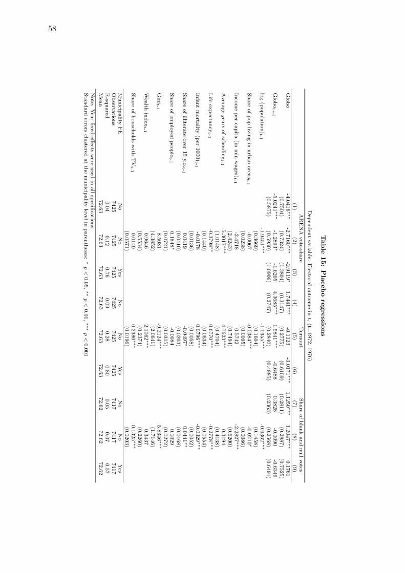
58
Table
15:
Pla
ceb
ore
gre
ssion
s
Dep
end
ent
varia
ble:
Electo
ral
ou
tcom
ein
t,(t=
1972,
1976)
AR
EN
Avote-sh
are
Tu
rnou
tSh
are
of
bla
nk
an
dnu
llvotes
(1)
(2)
(3)
(4)
(5)
(6)
(7)
(8)
(9)
Glo
bo
-4.0
416∗∗∗
-2.7
160∗∗∗
-2.9
119∗
1.7
441∗∗∗
-0.1
123
-3.0
171∗∗∗
1.1
250∗∗∗
1.2
047∗∗∗
0.1
761
(0.7
504)
(0.7
324)
(1.3
804)
(0.3
147)
(0.2
775)
(0.6
109)
(0.2
811)
(0.2
887)
(0.7
525)
Glo
bot+
1-5
.0241∗∗∗
-1.2
893∗
-1.6
205
4.3
685∗∗∗
1.5
841∗∗∗
-0.6
488
0.3
828
-0.0
090
-0.6
349
(0.5
875)
(0.5
930)
(1.0
906)
(0.2
747)
(0.2
840)
(0.4
885)
(0.2
363)
(0.2
568)
(0.6
491)
log
(pop
ula
tion)t-1
-1.9
451∗∗∗
-1.0
355∗∗∗
-0.9
362∗∗∗
(0.3
669)
(0.1
604)
(0.1
458)
Share
of
pop
livin
gin
urb
an
area
st-1
-0.0
067
-0.0
384∗∗∗
-0.0
210∗
(0.0
238)
(0.0
095)
(0.0
086)
Inco
me
per
capita
(inm
inw
ages)
t-1-2
.4718
0.5
742
-2.2
827∗∗∗
(2.4
243)
(0.7
494)
(0.6
200)
Avera
ge
yea
rsof
schoolin
gt-1
-5.3
017∗∗∗
4.7
623∗∗∗
0.3
194
(1.0
148)
(0.4
704)
(0.4
138)
Life
exp
ectan
cyt-1
-0.3
798∗∗
0.6
770∗∗∗
-0.2
778∗∗∗
(0.1
440)
(0.0
634)
(0.0
554)
Infa
nt
morta
lity(p
er1000)t-1
-0.0
178
0.0
796∗∗∗
-0.0
329∗∗∗
(0.0
136)
(0.0
058)
(0.0
052)
Share
of
illiterate
over
15
y.o.t-1
0.0
419
-0.0
497∗
0.0
441∗∗
(0.0
410)
(0.0
203)
(0.0
168)
Share
of
emp
loyed
peo
ple
t-10.1
848∗
-0.0
084
0.0
029
(0.0
721)
(0.0
315)
(0.0
272)
Gin
it-18.5
081
-9.2
124∗∗∗
5.8
346∗∗∗
(4.3
852)
(2.0
641)
(1.7
146)
Wea
lthin
dex
t-10.9
646
2.1
062∗∗∗
0.3
437
(0.5
534)
(0.2
374)
(0.2
260)
Share
of
hou
sehold
sw
ithT
Vt-1
0.0
149
0.2
380∗∗∗
0.1
325∗∗∗
(0.0
571)
(0.0
196)
(0.0
203)
Mu
nicip
ality
FE
No
No
Yes
No
No
Yes
No
No
Yes
Observ
atio
ns
7425
7425
7425
7425
7425
7425
7417
7417
7417
R-sq
uared
0.0
40.1
20.7
60.0
90.2
80.8
00.0
50.0
70.5
7M
ean
72.6
372.6
372.6
372.6
372.6
372.6
372.6
272.6
272.6
2
Note:
Yea
rfi
xed
-effects
were
used
inall
specifi
catio
ns
Sta
nd
ard
errors
clustered
at
the
mu
nicip
ality
level
inparen
theses:
∗p<
0.0
5,∗∗
p<
0.0
1,∗∗∗
p<
0.0
01
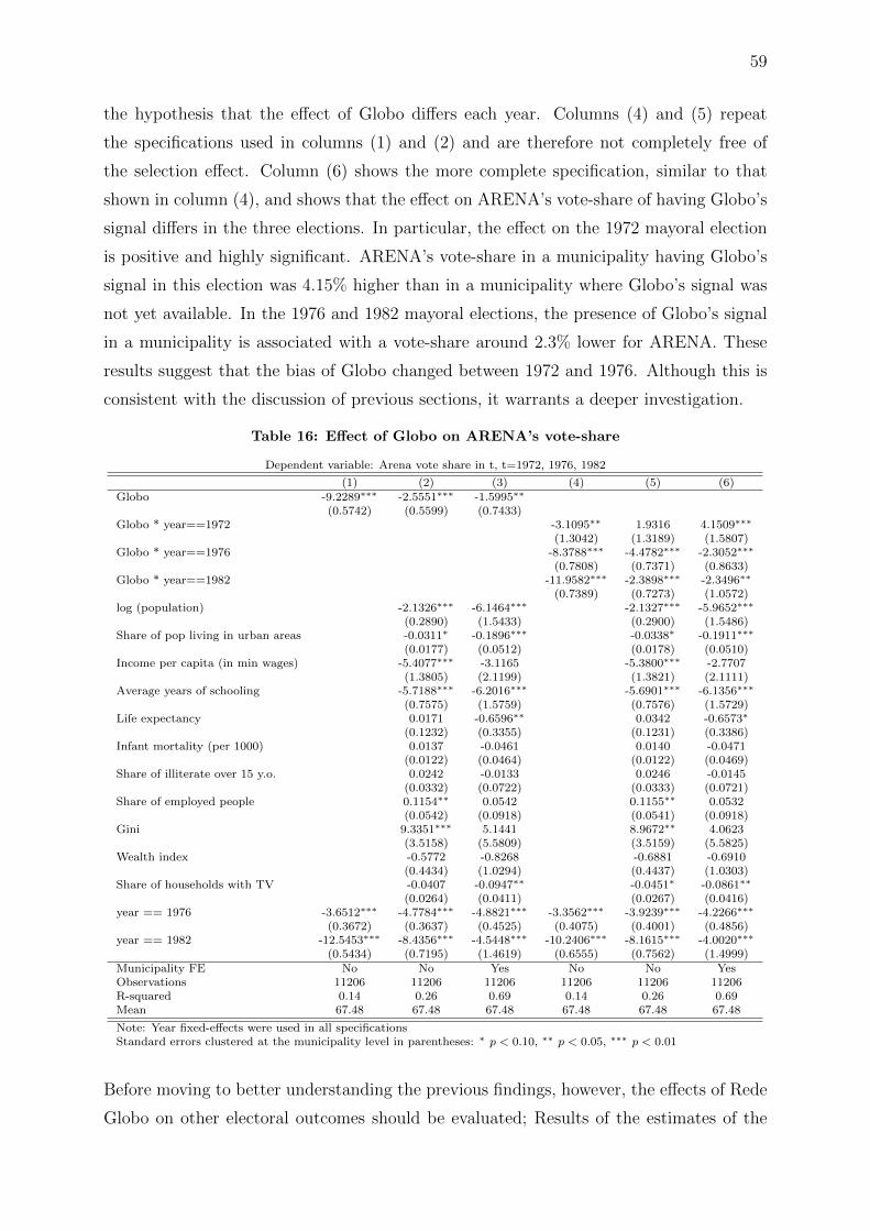
59
the hypothesis that the effect of Globo differs each year. Columns (4) and (5) repeat
the specifications used in columns (1) and (2) and are therefore not completely free of
the selection effect. Column (6) shows the more complete specification, similar to that
shown in column (4), and shows that the effect on ARENA’s vote-share of having Globo’s
signal differs in the three elections. In particular, the effect on the 1972 mayoral election
is positive and highly significant. ARENA’s vote-share in a municipality having Globo’s
signal in this election was 4.15% higher than in a municipality where Globo’s signal was
not yet available. In the 1976 and 1982 mayoral elections, the presence of Globo’s signal
in a municipality is associated with a vote-share around 2.3% lower for ARENA. These
results suggest that the bias of Globo changed between 1972 and 1976. Although this is
consistent with the discussion of previous sections, it warrants a deeper investigation.
Table 16: Effect of Globo on ARENA’s vote-share
Dependent variable: Arena vote share in t, t=1972, 1976, 1982
(1) (2) (3) (4) (5) (6)Globo -9.2289∗∗∗ -2.5551∗∗∗ -1.5995∗∗
(0.5742) (0.5599) (0.7433)Globo * year==1972 -3.1095∗∗ 1.9316 4.1509∗∗∗
(1.3042) (1.3189) (1.5807)Globo * year==1976 -8.3788∗∗∗ -4.4782∗∗∗ -2.3052∗∗∗
(0.7808) (0.7371) (0.8633)Globo * year==1982 -11.9582∗∗∗ -2.3898∗∗∗ -2.3496∗∗
(0.7389) (0.7273) (1.0572)log (population) -2.1326∗∗∗ -6.1464∗∗∗ -2.1327∗∗∗ -5.9652∗∗∗
(0.2890) (1.5433) (0.2900) (1.5486)Share of pop living in urban areas -0.0311∗ -0.1896∗∗∗ -0.0338∗ -0.1911∗∗∗
(0.0177) (0.0512) (0.0178) (0.0510)Income per capita (in min wages) -5.4077∗∗∗ -3.1165 -5.3800∗∗∗ -2.7707
(1.3805) (2.1199) (1.3821) (2.1111)Average years of schooling -5.7188∗∗∗ -6.2016∗∗∗ -5.6901∗∗∗ -6.1356∗∗∗
(0.7575) (1.5759) (0.7576) (1.5729)Life expectancy 0.0171 -0.6596∗∗ 0.0342 -0.6573∗
(0.1232) (0.3355) (0.1231) (0.3386)Infant mortality (per 1000) 0.0137 -0.0461 0.0140 -0.0471
(0.0122) (0.0464) (0.0122) (0.0469)Share of illiterate over 15 y.o. 0.0242 -0.0133 0.0246 -0.0145
(0.0332) (0.0722) (0.0333) (0.0721)Share of employed people 0.1154∗∗ 0.0542 0.1155∗∗ 0.0532
(0.0542) (0.0918) (0.0541) (0.0918)Gini 9.3351∗∗∗ 5.1441 8.9672∗∗ 4.0623
(3.5158) (5.5809) (3.5159) (5.5825)Wealth index -0.5772 -0.8268 -0.6881 -0.6910
(0.4434) (1.0294) (0.4437) (1.0303)Share of households with TV -0.0407 -0.0947∗∗ -0.0451∗ -0.0861∗∗
(0.0264) (0.0411) (0.0267) (0.0416)year == 1976 -3.6512∗∗∗ -4.7784∗∗∗ -4.8821∗∗∗ -3.3562∗∗∗ -3.9239∗∗∗ -4.2266∗∗∗
(0.3672) (0.3637) (0.4525) (0.4075) (0.4001) (0.4856)year == 1982 -12.5453∗∗∗ -8.4356∗∗∗ -4.5448∗∗∗ -10.2406∗∗∗ -8.1615∗∗∗ -4.0020∗∗∗
(0.5434) (0.7195) (1.4619) (0.6555) (0.7562) (1.4999)Municipality FE No No Yes No No YesObservations 11206 11206 11206 11206 11206 11206R-squared 0.14 0.26 0.69 0.14 0.26 0.69Mean 67.48 67.48 67.48 67.48 67.48 67.48
Note: Year fixed-effects were used in all specificationsStandard errors clustered at the municipality level in parentheses: ∗ p < 0.10, ∗∗ p < 0.05, ∗∗∗ p < 0.01
Before moving to better understanding the previous findings, however, the effects of Rede
Globo on other electoral outcomes should be evaluated; Results of the estimates of the

60
complete specification of equation 2.4 using voter turnout and the share of blank and null
votes as dependent variables are presented in Table 17.40 The average effect of Globo on
these voter outcomes is statistically zero, as seen in the coefficients in columns (1) and
(3). However, as Globo’s role over time changed dramatically, testing for heterogeneous
effects across different elections for these variables is also required. These results are
reported in columns (2) and (4). The effect of Globo on voter turnout changes greatly
over different elections. In 1972, the point estimate is negative, but the effect is not
significant, probably due to the small number of municipalities with Globo’s signal at the
time. In 1976, the point estimate is still negative, but smaller and significant. In 1982,
the effect becomes positive and highly significant, suggesting the influence of television in
the political process increased over time. The effects on the share of blank and null votes
are zero in the three elections studied.
Table 17: Effect of Globo on turnout and share of blank and null votes
Dependent variable: Electoral outcome in t, t=1972, 1976, 1982
Turnout Share of blank and null votes(1) (2) (3) (4)
Globo 0.1308 -0.1048(0.3110) (0.3239)
Globo * year==1972 -0.9373 -0.2052(0.5757) (0.8041)
Globo * year==1976 -0.7704∗∗ -0.0504(0.3254) (0.3922)
Globo * year==1982 1.2665∗∗∗ -0.1323(0.4466) (0.4088)
log (population) -2.8995∗∗∗ -2.7589∗∗∗ 2.2367∗∗∗ 2.2264∗∗∗
(0.6664) (0.6614) (0.5525) (0.5538)Share of pop living in urban areas -0.0276 -0.0285 0.0210 0.0211
(0.0191) (0.0189) (0.0175) (0.0175)Income per capita (in min wages) 1.9884∗∗∗ 1.7987∗∗∗ -2.0102∗∗∗ -2.0111∗∗∗
(0.5792) (0.5832) (0.5920) (0.5933)Average years of schooling -0.7347 -0.7005 0.8541 0.8511
(0.6424) (0.6394) (0.6209) (0.6209)Life expectancy 0.3350∗∗ 0.2791∗∗ -0.2930∗∗ -0.2908∗∗
(0.1345) (0.1352) (0.1336) (0.1349)Infant mortality (per 1000) 0.0432∗∗ 0.0359∗ -0.0442∗∗ -0.0438∗∗
(0.0188) (0.0189) (0.0180) (0.0182)Share of illiterate over 15 y.o. -0.0569∗ -0.0569∗ 0.0532∗ 0.0532∗
(0.0318) (0.0318) (0.0296) (0.0296)Share of employed people 0.0295 0.0273 -0.0335 -0.0333
(0.0375) (0.0376) (0.0332) (0.0332)Gini -8.4621∗∗∗ -7.7513∗∗∗ -0.4997 -0.5011
(2.2927) (2.2978) (2.2002) (2.1951)Wealth index -0.0521 -0.1358 1.0406∗∗∗ 1.0406∗∗∗
(0.3978) (0.3971) (0.3754) (0.3770)Share of households with TV -0.0466∗∗∗ -0.0601∗∗∗ 0.0095 0.0098
(0.0148) (0.0153) (0.0144) (0.0149)year == 1976 3.9650∗∗∗ 4.1023∗∗∗ -4.2058∗∗∗ -4.2278∗∗∗
(0.2012) (0.2218) (0.2624) (0.2851)year == 1982 4.9059∗∗∗ 4.4822∗∗∗ -1.4751∗∗ -1.4715∗∗
(0.5816) (0.5956) (0.5734) (0.5819)Municipality FE Yes Yes Yes YesObservations 11209 11209 11200 11200R-squared 0.72 0.72 0.43 0.43Mean 79.91 79.91 8.45 8.45
Note: Year and municipality fixed-effects were used in all specificationsStandard errors clustered at the municipality level in parentheses: ∗ p < 0.10, ∗∗ p < 0.05, ∗∗∗ p < 0.01
40The complete set of results is presented in appendix B, Tables 36 and 37.

61
2.5.3 Heterogeneity by socioeconomic characteristics
This subsection analyzes the possibility that the effects of exposure to Globo may be
heterogeneous along the dimensions of education – measured by average years of schooling
– and the share of households with televisions in the municipality. The idea behind this
tests is to provide more clear evidence that the effects documented in the previous tables
are indeed related to the presence of Globo. As already discussed, if one crucial reason
behind television’s influence in Brazil is the strength of the country’s oral tradition, the
effect of Globo should be more accentuated in municipalities with lower average years
of schooling. Also, if the effect is indeed related to television, it should also be more
accentuated in municipalities with a higher share of households with television.
Because the effect of Globo is heterogeneous on the year dimension, Equation 2.5 is
estimated with interaction with year dummies. Time–varying control, municipality and
year fixed–effects and all relevant interactions, though not reported, are included in the
regressions. Results are shown in Table 18. Column (1) presents the estimates interacting
average years of schooling at the municipality with the presence of Globo. According to
what has been discussed, Globo’s effect is expected to be less emphasized in municipalities
with higher average years of schooling. However, whether this is true is not clear. The
effect in 1972, for instance, is stronger in municipalities with higher average of years of
schooling.
Column (2) shows estimates interacting the share of households with televisions with the
presence of Globo. In this case, the coefficients associated with the interactions should
go in the same direction as the coefficients associated with the Globo effect itself. Again,
this may not be the case. The effect in 1982 is weaker in municipalities with a higher
share of households with televisions.
One possible reason for these unclear results might be that average years of schooling at
the municipality level and the share of households with televisions are highly positively
correlated41 but are expected to have different effects in the interaction with Globo. To
overcome this possible issue of omitted variable bias, the estimation is done including
the interactions with both observables. The results shown in column (3) are much more
intuitive, even though most coefficients are not statistically significant when tested indi-
41In fact, the correlation between these two variables is 0.825 in the estimating sample.
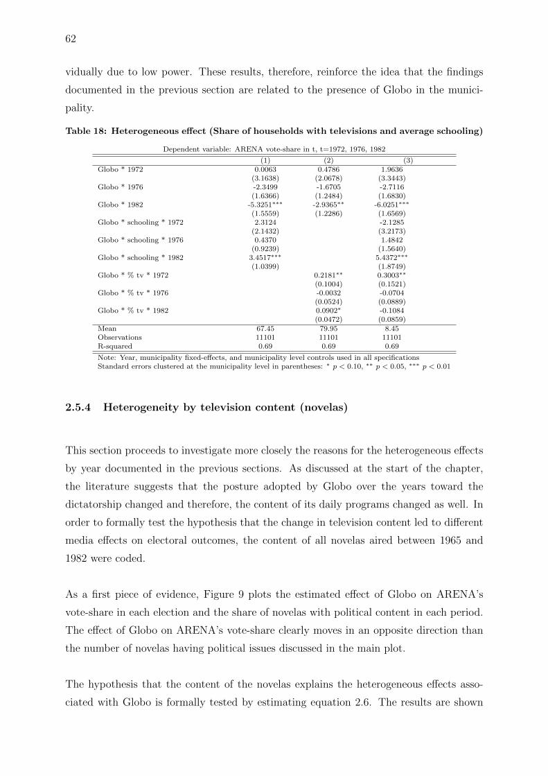
62
vidually due to low power. These results, therefore, reinforce the idea that the findings
documented in the previous section are related to the presence of Globo in the munici-
pality.
Table 18: Heterogeneous effect (Share of households with televisions and average schooling)
Dependent variable: ARENA vote-share in t, t=1972, 1976, 1982
(1) (2) (3)Globo * 1972 0.0063 0.4786 1.9636
(3.1638) (2.0678) (3.3443)Globo * 1976 -2.3499 -1.6705 -2.7116
(1.6366) (1.2484) (1.6830)Globo * 1982 -5.3251∗∗∗ -2.9365∗∗ -6.0251∗∗∗
(1.5559) (1.2286) (1.6569)Globo * schooling * 1972 2.3124 -2.1285
(2.1432) (3.2173)Globo * schooling * 1976 0.4370 1.4842
(0.9239) (1.5640)Globo * schooling * 1982 3.4517∗∗∗ 5.4372∗∗∗
(1.0399) (1.8749)Globo * % tv * 1972 0.2181∗∗ 0.3003∗∗
(0.1004) (0.1521)Globo * % tv * 1976 -0.0032 -0.0704
(0.0524) (0.0889)Globo * % tv * 1982 0.0902∗ -0.1084
(0.0472) (0.0859)Mean 67.45 79.95 8.45Observations 11101 11101 11101R-squared 0.69 0.69 0.69
Note: Year, municipality fixed-effects, and municipality level controls used in all specificationsStandard errors clustered at the municipality level in parentheses: ∗ p < 0.10, ∗∗ p < 0.05, ∗∗∗ p < 0.01
2.5.4 Heterogeneity by television content (novelas)
This section proceeds to investigate more closely the reasons for the heterogeneous effects
by year documented in the previous sections. As discussed at the start of the chapter,
the literature suggests that the posture adopted by Globo over the years toward the
dictatorship changed and therefore, the content of its daily programs changed as well. In
order to formally test the hypothesis that the change in television content led to different
media effects on electoral outcomes, the content of all novelas aired between 1965 and
1982 were coded.
As a first piece of evidence, Figure 9 plots the estimated effect of Globo on ARENA’s
vote-share in each election and the share of novelas with political content in each period.
The effect of Globo on ARENA’s vote-share clearly moves in an opposite direction than
the number of novelas having political issues discussed in the main plot.
The hypothesis that the content of the novelas explains the heterogeneous effects asso-
ciated with Globo is formally tested by estimating equation 2.6. The results are shown
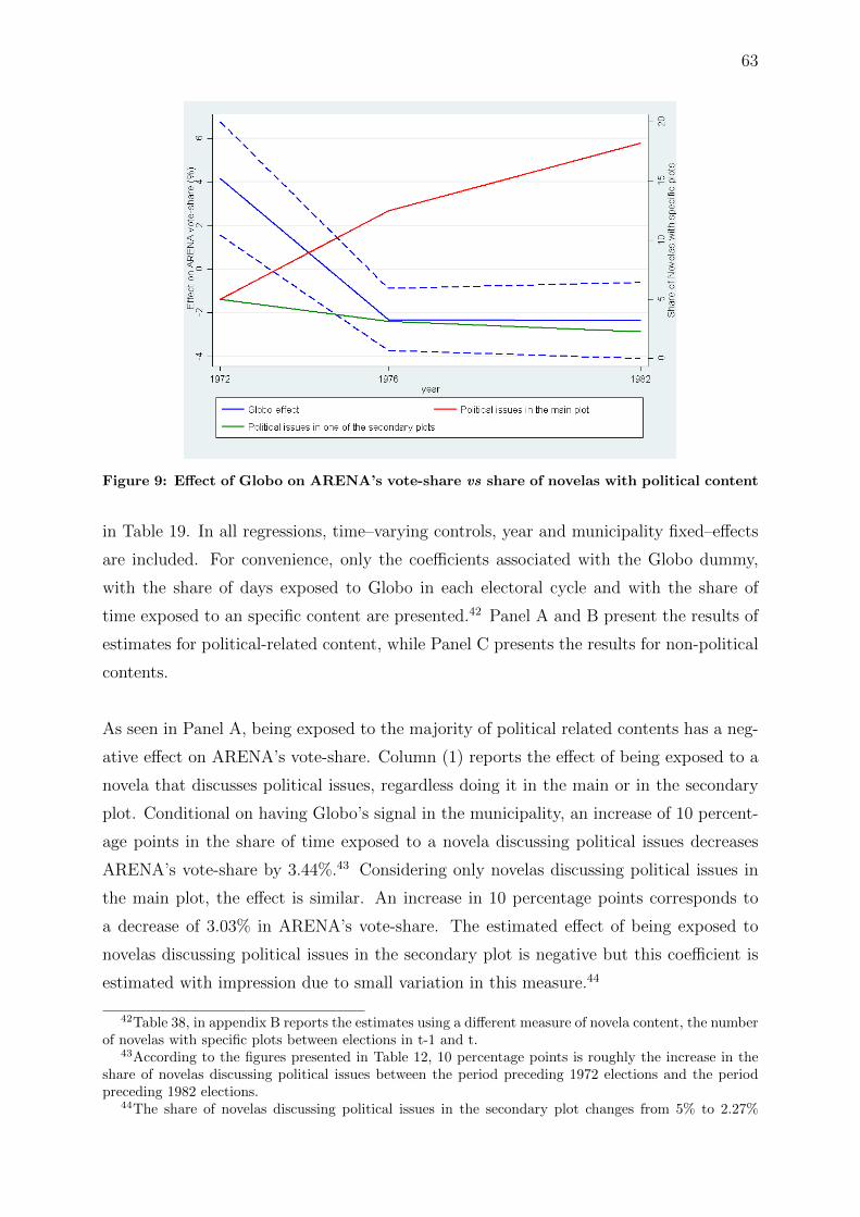
63
Figure 9: Effect of Globo on ARENA’s vote-share vs share of novelas with political content
in Table 19. In all regressions, time–varying controls, year and municipality fixed–effects
are included. For convenience, only the coefficients associated with the Globo dummy,
with the share of days exposed to Globo in each electoral cycle and with the share of
time exposed to an specific content are presented.42 Panel A and B present the results of
estimates for political-related content, while Panel C presents the results for non-political
contents.
As seen in Panel A, being exposed to the majority of political related contents has a neg-
ative effect on ARENA’s vote-share. Column (1) reports the effect of being exposed to a
novela that discusses political issues, regardless doing it in the main or in the secondary
plot. Conditional on having Globo’s signal in the municipality, an increase of 10 percent-
age points in the share of time exposed to a novela discussing political issues decreases
ARENA’s vote-share by 3.44%.43 Considering only novelas discussing political issues in
the main plot, the effect is similar. An increase in 10 percentage points corresponds to
a decrease of 3.03% in ARENA’s vote-share. The estimated effect of being exposed to
novelas discussing political issues in the secondary plot is negative but this coefficient is
estimated with impression due to small variation in this measure.44
42Table 38, in appendix B reports the estimates using a different measure of novela content, the numberof novelas with specific plots between elections in t-1 and t.
43According to the figures presented in Table 12, 10 percentage points is roughly the increase in theshare of novelas discussing political issues between the period preceding 1972 elections and the periodpreceding 1982 elections.
44The share of novelas discussing political issues in the secondary plot changes from 5% to 2.27%
64
Still in Panel A, the results of being exposed to a novela with a character in opposition to
the ruling party or to a political powerful group are presented in columns (4) and (5). If the
novela have a main character of this type, the effect on ARENA’s vote-share is negative; an
increase of 10 percentage points in the share of time exposed reduces ARENA’s vote-share
by 4.41%. On the other hand, if the novela has a “political character” who is not its main
character, the same variation in exposure time is associated with an increase of 7.15%
on ARENA’s vote-share. Although counterintuitive, this result can be easily understand
by looking at Figure 9 and at Table 12. Over time, a substitution clearly occurred in
which the number of novelas discussing political issues in the main plot increased, and
the number of novelas discussing political issues in their seconday plots decreased. The
result in column (5), therefore, can be understand as been a result of omitting the measure
of exposure used in column (4).
Panel B shows the effects of exposure to novelas discussing specific political issues. Expo-
sure to all the listed issues have a negative and significant effect on ARENA’s vote-share.
Interestingly, novelas that discuss demand for democracy are among the ones with higher
(negative) effect on ARENA’s vote-share.
Panel C, in turn, shows the effects of exposure to issues that are not necessarily connected
to politics. Excluding novelas that have rural plots and those discussing slavery, exposure
to other issues have no significant effects on ARENA’s vote-share. Note that the inter-
action of measures of novela content with Globo are estimated separately; therefore, the
negative effects of non-political-related issues do not necessarily mean that novelas with
rural plots per se are directly causing a negative effect on ARENA’s vote-share. It may
be the case that a relevant part of the novelas discussing political issues took place in a
rural setting.45
2.6 Conclusion
This chapter investigated the presence of media capture during the Brazilian dictatorship.
This was accomplished by evaluating the effects of Globo, the main Brazilian television
station, on mayoral electoral outcomes during in the 1970s and 1980s.
between the period preceding 1972 elections and the one preceding 1982 elections.45Indeed, this is the case of some of novelas that discussed political issues; for example, the case of O
Bem Amado and Irmaos Coragem.

65
Table
19:
Hete
rogeneous
eff
ects
by
novela
conte
nt
Dep
end
ent
vari
ab
le:
AR
EN
A’s
vote
-share
inm
unic
ipal
elec
tion
sin
t,t=
1972,
1976,
1982
Conte
nt
mea
sure
:S
hare
of
tim
eex
pose
dto
an
ovel
aw
ith
asp
ecifi
cp
lot
bet
wee
nel
ecti
on
sin
t-1
an
dt.
PanelA:Politicalrelate
dplots
(part1
)
Politi
cal
issu
esP
oliti
cal
issu
es(m
ain
plo
t)P
oliti
cal
issu
es(s
econ
dary
plo
t)P
oliti
cal
chara
cter
(main
)P
oliti
cal
chara
cter
(sec
on
dary
)(1
)(2
)(3
)(4
)(5
)G
lob
o-1
.2290
-1.4
049
-0.6
633
-1.1
963
-1.4
860
(0.9
200)
(0.9
245)
(0.9
765)
(0.9
229)
(0.9
429)
Share
of
days
exp
ose
dto
Glo
bo
0.0
650∗∗
0.0
441
0.0
098
0.0
439
-0.0
436∗∗
(0.0
305)
(0.0
275)
(0.0
220)
(0.0
269)
(0.0
203)
Exp
osu
reto
spec
ific
novel
aco
nte
nt
-0.3
436∗∗
∗-0
.3026∗∗
-0.6
092
-0.4
410∗∗
∗0.7
237∗∗
(0.1
147)
(0.1
202)
(0.4
443)
(0.1
705)
(0.3
644)
Obse
rvati
on
s11206
11206
11206
11206
11206
R-s
qu
are
d0.6
90.6
90.6
90.6
90.6
9M
ean
67.4
867.4
867.4
867.4
867.4
8
PanelB:Politicalrelate
dplots
(part2
)C
orr
upti
on
Ele
ctio
ns
Pub
lic
reso
urc
esD
emocr
acy
Oth
erp
oliti
cal
issu
es(1
)(2
)(3
)(4
)(5
)G
lob
o-0
.6609
-0.5
643
-1.0
102
-0.7
593
-1.5
065
(0.9
591)
(0.9
586)
(0.9
232)
(0.9
349)
(0.9
218)
Share
of
days
exp
ose
dto
Glo
bo
-0.0
060
0.0
019
0.0
015
0.0
152
0.0
635∗∗
(0.0
146)
(0.0
158)
(0.0
152)
(0.0
173)
(0.0
296)
Exp
osu
reto
spec
ific
novel
aco
nte
nt
-0.1
685∗
-0.2
468∗∗
-0.3
351∗∗
∗-0
.3280∗∗
∗-0
.3868∗∗
∗
(0.0
915)
(0.1
094)
(0.1
220)
(0.1
096)
(0.1
272)
Obse
rvati
on
s11206
11206
11206
11206
11206
R-s
qu
are
d0.6
90.6
90.6
90.6
90.6
9M
ean
67.4
867.4
867.4
867.4
867.4
8
PanelC:Non-p
oliticalplots
His
tori
cal
Ru
ral
Per
ipher
yP
reju
dic
eS
laver
y(1
)(2
)(3
)(4
)(5
)G
lob
o-0
.8851
-0.8
527
-1.1
332
-0.8
649
-1.1
288
(0.9
213)
(0.9
364)
(0.9
219)
(0.9
733)
(0.9
212)
Share
of
days
exp
ose
dto
Glo
bo
-0.0
594∗
0.0
139
0.0
039
-0.0
344
0.0
151
(0.0
334)
(0.0
202)
(0.0
202)
(0.0
339)
(0.0
185)
Exp
osu
reto
spec
ific
novel
aco
nte
nt
0.1
920
-0.0
635∗∗
-0.0
644
0.0
401
-0.3
160∗∗
(0.1
347)
(0.0
316)
(0.0
516)
(0.0
622)
(0.1
280)
Obse
rvati
on
s11206
11206
11206
11206
11206
R-s
qu
are
d0.6
90.6
90.6
90.6
90.6
9M
ean
67.4
867.4
867.4
867.4
867.4
8
Sta
nd
ard
erro
rscl
ust
ered
at
the
mu
nic
ipality
level
inpare
nth
eses
:∗p<
0.1
0,∗∗
p<
0.0
5,∗∗
∗p<
0.0
1

66
To identify such effects, this chapter explored differences in the timing of Globo’s entry
into different municipalities. The main empirical challenge is that Globo’s entry could
be correlated with political preferences at the municipality level. Evidence provided in
this chapter shows that conditional on a set of municipality–level controls as well as
municipality and year fixed-effects, there is no evidence of a politically driven entry of
Globo.
The main results show that Globo has an average negative effect on ARENA’s vote-
share in the three mayoral elections occurring between 1972 and 1982. This effect is
heterogeneous in the year dimension. Globo has a positive effect on ARENA’s vote-share
in the first elections studied in this chapter, in 1972, and then in the later years, the
effect becomes negative. In order to better understand this shifting in the effect of Globo,
the content of Brazilian novelas were coded and used in the analysis. The result of the
regressions using this data show that exposure to novelas with politically-related content
has a negative effect on ARENA’s vote-share.
These results are consistent with the anecdotal evidence suggesting that in response to the
new context of political and economic crisis, Globo assumed a critical role in the last years
of the regime. They are also consistent with a theoretical result by Prat & Stromberg
(2011), according to which the presence of a news-related profit motive makes political
capture of media vehicles more difficult to happen.
67
3 POLITICAL PREACHING IN THE CLASSROOM: EVIDENCE FROMTEACHERS’ PARTY AFFILIATION IN BRAZILIAN PUBLIC SCHOOLS
3.1 Introduction
Frequently regarded as one of the crucial inputs in the educational process (Rockoff
(2004)), teachers commonly stand among the politically engaged groups with the most
influence on shaping essential public policies and on promoting economic and social de-
velopment.46 However, a seemingly underappreciated topic by both the economics and
political science literatures has been the role that politically active teachers might per-
form in political environments and especially the influence they may exert on the electoral
process. Despite the suggestion by contemporary observers that faculty would be indoc-
trinating students with certain politically bent education (Horowitz (2006)), the literature
on political behavior has focused on exploring the effect on students’ political attitudes
stemming from education acquisition as a whole (Persson (2014), Kam & Palmer (2008a)),
with no special regard for the particular influence of partisan political preaching by teach-
ers with strong political views. It seems natural to think, though, that while facing great
audiences of recently registered voters and individuals that just got into political question-
ing, teachers may play a unique and important part not only in their students’ political
(and partisan) stances, but also in the configuration of electoral outcomes. At the very
least, they hold a prime position to discuss political matters with their students; how-
ever, they could also present themselves as self-appointed party delegates trying to deliver
their students’ votes, or even as political power brokers involved in clientelistic relation-
ships47 - especially in the developing world, where these practices tend to be widespread.48
Notwithstanding, little has been reported on the extent to which teachers are able to in-
fluence voting behavior.
This chapter investigates this issue by looking at the effects of the presence of party-
affiliated teachers on certain regions’ electoral outcomes. Merging a unique individual
level database of public high school teachers in Sao Paulo, Brazil, with an individual level
database of party-affiliated voters, it is possible to identify high school teachers’ politi-
46In the context of teachers’ unionisation, for instance, it has been argued that the acquisition ofbargaining power by such agents may have important consequences on resource allocation in publicschools (Hoxby (1996); Moe (2011)).
47The case for contexts of education provision as particularly prone for the flourishing of patronage ismade by Corrales (2006), for instance.
48See, for instance, Kitschelt & Wilkinson (2007) and Schaffer (2007).

68
cal affiliations. Furthermore, a very rich database of electoral outcomes and electorate
characteristics is exploited to investigate the relationship between the density of affiliated
teachers and the electoral outcomes at a highly disaggregated geographic level, which
allows to get high precision estimates and avoid certain endogeneity issues.
The matter of such an influence by teachers poses as a very relevant question for two main
reasons. First, while it may be hard to believe that teachers alone are able to change the
outcome of a plurality election by influencing their students’ voting behaviour, the same
is not true for proportional elections, in which the number of votes necessary for being
elected might be much smaller, especially in small municipalities. The second reason relies
on the fact that evidence on such influence would be a sign that teachers are diverging
from the curriculum content standards, which may not only affect electoral outcomes, but
also have deleterious effects on education outcomes.49
This research is presented with important empirical challenges, especially concerning the
matter of selection in the assignment of teachers to schools. To overcome this issue,
the varying intensity of the hypothesized effect according to electorate characteristics
at the polling station level, the specific place in the polling district where each voter is
designed to cast his or her vote, is exploited. The underlying hypothesis is that teachers
- or voters in general - are not able to select themselves at that level in any manner,
and thus controlling for specific characteristics of regions where selection may yet occur
should render estimates free of that kind of selection bias. Evidence of a positive and
significant effect of the presence of affiliated teachers on the electoral performance of the
corresponding party through influencing their voting-aged students is found. Moreover,
the results show this effect is more pronounced in plurality elections and appear to be
restricted to teachers affiliated to the Workers’ Party. For that party, it is also found
evidence that affiliated teachers do not have an impact on electoral turnout by students;
rather, these teachers are suggested to alter the political preferences of students that
would vote for another party.
This paper communicates with at least two different strands of the political economy
and political science literatures, as well as to the education literature. First, it is closely
related to studies focused on exploring the relationship between education and political
participation. Extensive research on this topic has traditionally documented a strong and
49In the context of unionisation, deleterious effects on student performance have been documented byHoxby (1996) and Eberts & Stone (1987).

69
positive relationship between schooling and political participation: Hillygus (2005), Nie,
Junn & Stehlik-Barry (1996) and Wolfinger & Rosenstone (1980), for instance, suggest
the connection of higher education to an enhanced voter turnout, political knowledge and
civic engagement.50 On the other hand, a more rigid exploration of the corresponding
causal link has only been developed by more recent work, with mixed findings. While
Dee (2004) and Milligan, Moretti & Oreopoulos (2004) find a positive effect using U.S.
and U.K. data, Persson (2014) and Kam & Palmer (2008b) using data from the same
countries, and Solis (2013) using data from Chile suggest that the relationship between
education and political participation is spurious.
Differently from that literature, however, this paper aims to study the influence of spe-
cific behavior by a particular group of teachers, namely the political indoctrination of
students by their party-affiliated teachers. In this sense, this work is also related to the
literature on education as fundamentally a political process and on teachers’ behavior
in classroom situations.51 Under a comparative education approach, Hahn (1998) and
Westheimer & Kahne (2008) argue that diversified practices of citizenship education -
arguably the subject area most favorable to engagement with political issues - are highly
influenced by national political scenarios and driven by different beliefs about democracy,
while Schugurensky & Myers (2003) stress teachers’ political participation as an impor-
tant consideration for understanding such practices. In a case study of Brazilian and
Canadian secondary teachers, Myers (2007) illustrates the influence of political participa-
tion - measured according to involvement in teachers’ unions, political parties and social
movements - on both pedagogical and curricular approaches.
Lastly, the present work is also related to the political clientelism literature, which ex-
plores how and under what conditions certain agents - voters or political power brokers -
trade their political support during elections, as well as the inefficiencies stemming from
their corresponding rewards. In the context of developing countries, for instance, Finan
(2004) presents an example of that practice by arguing that federal deputies in Brazil
reward municipalities based on their political support. Regarding the Brazilian educa-
tional context, Mainwaring (1999) reports that, as a result of clientelism, in the state of
Bahia about 37,000 teachers who were on the public payroll in 1987 had never taught
a single class. On the other hand, the more specific analysis of the situations in which
political brokers may arise - and what kind of individuals are more likely to play that role
50This hypothesized effect of educational attainment has sometimes been used to advocate governmentintervention in the education market (Hanushek (2002)).
51See also Ginsburg et al. (1992).

70
- and act to influence electoral outcomes as middlemen between political parties and large
groups of voters seems not yet thoroughly developed nor fully understood. One exception
is provided by Larreguy (2013), where the establishment of clientelistic networks by com-
munal land leaders in Mexico serves as the basis for an investigation of the monitoring
capabilities presented by political parties in securing their votes.
The remainder of this chapter is organized as follows. Section 3.2 describes voting proce-
dures in Brazilian elections and the assignment of teachers and students to public schools
in Sao Paulo. Section 3.3 describes the data and the empirical strategy. Sections 3.4 and
3.5 discuss the main results, and Section 3.6 concludes.
3.2 Institutional Background
This section highlights the main features of the Brazilian electoral system and characterize
the public education system in the state of Sao Paulo52 - for which data on teachers
are available - placing particular emphasis on the rules governing student and teacher
placement in public schools.
3.2.1 Voting in Brazil
Brazilian states and municipalities have autonomous administrations, and both executive
leaders and local legislatures are elected by direct elections. Voting is mandatory for
literate citizens aged 18-70 and facultative for citizens between 16 and 17 or over 70,
and for illiterate people. Elections in Brazil are held every four years. Elections for
president, senators, deputies and governors are held jointly while elections for mayors and
city councilmen are staggered by two years relative to general elections.
In order to better organize election procedures, each state is divided into polling districts
(Zona Eleitoral) which are, in their turn, composed of several polling stations (Secao
Eleitoral). Polling districts have their limits defined according to geographical and de-
mographic characteristics and are managed by electoral offices charged with taking care
of electoral registers; Figures 12 and 13 in the appendix illustrate the distribution of mu-
52Sao Paulo is the wealthiest and most developed state in Brazil, with a population of over 44 millionpeople and a territorial area close to 250,000 km2, equivalent to the area of the state of Michigan or tothe United Kingdom.

71
nicipalities within the state of Sao Paulo and the distribution of polling districts within
the city of Sao Paulo. A polling station, on the other hand, consists of a very specific
place in the polling district where each voter is designated to cast his or her vote, usually
a specific room in a school or public service center. Buildings (polling places) with one
of such polling stations tend, of course, to contain several ones. As such, polling stations
represent a highly disaggregated level of observation. Figures 14 and 15 in appendix C
provide a depiction of a polling place and a polling station, respectively, and Figure 10
below sums up the administrative hierarchy of electoral procedures in Brazil.
Figure 10: Administrative Hierarchy of Electoral Procedures in Brazil
State Polling district Polling place Polling station
In addition, Brazilian legislation (Codigo Eleitoral, art. 117) dictates that polling stations
have at most 400 voters in the states’ capital cities or 300 voters in other cities, and at
least 50 voters.53 Electoral laws also depict an effort of minimizing the distance between
voters’ places of residence and the polling stations to which they are assigned: at the time
of electoral registration, voters are able to express their preferences over polling places (but
not over specific polling stations) in the polling district of their residence, and they are
also prohibited from choosing a polling place from a different polling district (Resolucao
TSE 21,538/2003, art. 9).54
3.2.2 The Brazilian Public Educational System
Public education in Brazil is free of charge to all Brazilian citizens and can be provided
by municipalities, states or the federal government, depending on the level of education.
The pre-college educational system is arranged into four levels: preschool (attended by
6 year-olds), primary school (attended by 7 to 10 year-olds), secondary school (attended
53However, the same legislation also authorizes the regional electoral courts to surpass these limits inexceptional circumstances.
54In private communications, a former employee of a regional electoral authority has stated that eachvoter is automatically allocated to the polling station with the lower number of voters among thosestations in the polling place chosen by the voter.

72
by 11 to 14 year-olds) and high school (attended by 15 to 17 year-olds). Since the main
goal of this research is to investigate the influence teachers may present on students’
voting patterns, the analysis is focused on the high school level, which comprises students
qualified for voting.55
Even though Sao Paulo’s public education system is one of the best in Brazil, it is far
from the quality level presented in developed countries, which induces wealthier families
to obtain education services from private schools. Nonetheless, the cost of education in
private schools is extremely prohibitive for Brazilian standards; thus, around 85% of the
students that achieve high school completion in Brazil do so in public schools.56
3.2.3 Student and Teacher Placement in Sao Paulo’s Public Schools
The assignment of students to state high schools is regulated by state laws which funda-
mentally determine that students residing in a given school’s area of influence57 receive
priority in filling that school’s class vacancies. The minimum distance criterion is natu-
rally also the first to be considered in the placement of students that do not get to be
enrolled in the school that is closest to their homes.
Teacher assignment to these schools, in its turn, occurs on the basis of tests conducted at
the state level and specific to the school subject the applicant desires to teach. Applicants
must achieve a pre-established minimum score in order to be considered apt for teaching,
and those that do so are ranked according to their final score.58 A first group of top
ranked candidates are then summoned for a session where they select their most preferred
school among those with positions still available. School choice is made by one candidate
at a time, and priority in that procedure follows the candidates’ ranking (better ranked
candidates get to pick their schools first). In the event that not all teacher positions are
filled, new groups of lower ranked candidates are summoned for new school choice sessions
55High school education is usually provided by the state government, as directed by the BrazilianConstitution.
56Source: INEP. Available at <http://portal.inep.gov.br/rss\censo-escolar/-/asset\publisher/oV0H/content/id/19910>.
57The area of influence of a given public (high) school is defined to be (roughly) the region to whichthe school consists of the closest public (high) school.
58Applicants must hold an academic degree called a license, obtained through the completion of specificcollege courses with a stronger emphasis on teaching methods and pedagogy than those leading to abachelor’s degree. Additional academic degrees like master’s or doctorate degrees also contribute to thecandidate’s final score.

73
until all positions have been filled or all ranked candidates have been summoned. From
2004 to 2008, more than 26,000 positions were opened for basic education (i.e. secondary
and high school level) teachers in public schools managed by the state.
3.3 Data and Estimation Framework
The present analysis relies on several sources of data. In order to obtain information on
teachers’ political affiliation, individual level data - from the Sao Paulo State Department
of Education - on public high school teachers in Sao Paulo’s state-managed schools from
2008 to 2010 is combined with individual level information on politically affiliated voters
for the same years, provided by the federal electoral authority (TSE). It is possible thus
to identify, for each of those years, which of those teachers are affiliated, as well as the
political party to which they are affiliated. In particular, a teacher is defined to be affiliated
if it is possible to match his or her name to that of an affiliated voter who appears in
the affiliated voter list for the corresponding year. Moreover, it is also used data - also
provided by the TSE - on parties’ electoral outcomes at the polling station level and on
characteristics of voters allocated to each polling station.
The study of the relationship between the density of teachers affiliated to a given party and
electoral outcomes for that party is made through the construction of measures of political
affiliation at the level of regions consisting of intersections between polling districts and
municipalities.59 This is done in order to gain more variation in the main independent
variable, since there are 423 polling districts in the State of Sao Paulo as defined by
the electoral authorities, whereas considering the intersection between polling districts
and municipalities results in 790 units of observation. For brevity, such intersections
will henceforth be referred to as polling districts, and originally-defined districts will be
referred to as “TSE districts” should that need arise. This strategy also allows to have
a more reasonable measure of the density of party-affiliated teachers as it imposes the
restriction that students voting in a given municipality are most likely influenced by
teachers in that municipality (but not by teachers in the same TSE district and in other
municipalities). A deeper description of the relationship between the distributions of TSE
districts and municipalities in the state of Sao Paulo is given in Tables 39 and 40 in
appendix C.
59Each originally-defined district may either cover more than one municipality, have its area coincidewith one, or be a smaller part of a municipality. Source: http://www.tse.jus.br/eleitor/zonas-eleitorais.

74
The construction of measures of density of politically affiliated teachers would be a simple
task if information on geographic limits of each of the TSE polling districts were available.
Unfortunately, this is not the case. To circumvent this problem georeferencing algorithms
are used to match each state school to its closest polling place in the same municipality.
Then, each school is associated to the polling district corresponding to the matched polling
place. Finally, for each district the proportion of teachers affiliated to each political party
is computed.
Although the polling district is not the most disaggregated level at which it is possible to
explore regional variation in the density of affiliated teachers, it is the most disaggregated
level at which it is possible to credibly match that variation to the variation in electoral
outcomes. For instance, an alternative approach would be to consider only those (state-
managed) schools that are used as polling places during elections and associate party-
affiliated teachers with electoral outcomes at the school level. This approach, however,
imposes the strong restriction that students vote at the school where they study. As
not all polling places are state-managed high schools, restricting the analysis to such
schools would impose a selection problem that could compromise the interpretation of the
estimated coefficients.
Before describing the empirical strategy, it is convenient to present some statistics related
to the main independent variables, namely the share of high school teachers that are
affiliated to each political party. The corresponding figures are displayed in Table 20.
The analysis is restricted to the four parties with the highest numbers of affiliated teach-
ers at the state level: the Workers Party (PT), the Brazilian Social Democratic Party
(PSDB), the Brazilian Labour Party (PTB) and the Brazilian Democratic Movement
Party (PMDB). The PT is currently one of the most important parties in the Brazilian
political scenario, governing at the federal level since 2003. The PSDB has been the PT’s
main opposition in the federal government and has been ruling the state of Sao Paulo
since 1995, having PT as one of its main rivals at that state. The PTB has not shown
great representation in the chamber of deputies and neither has it elected any governor
in the last general election, but its relatively high number of affiliated teachers might be
explained by its association with unions and labor organizations. In its turn, the PMDB is
currently one of the biggest political parties in Brazil, being the second with more elected
members in the chamber of deputies.

75
Table 20: Share of Teachers Affiliated to Each Party
Political Party 2008 2010
PT 1.98% 2.03%
PSDB 0.99% 0.93%
PTB 0.67% 0.65%
PMDB 0.62% 0.62%
PV 0.43% 0.45%
PSB 0.37% 0.35%
PPS 0.37% 0.32%
PP 0.35% 0.32%
DEM 0.35% 0.31%
PDT 0.33% 0.32%
PR 0.32% 0.31%
Others 1.39% 1.50%
Number of High School Teachers 94,277 98,594
Note: the shares of affiliated teachers are relative to the totalof high school teachers in Sao Paulo’s public schools.
The identification strategy resembles the approaches taken by Duflo (2001) and Card
(1992) as variation in two dimensions that jointly determine the exposure of voters to
affiliated teachers is exploited, in a difference-in-differences (DD) setup. As mentioned
above, the first dimension, regarding“treatment intensity”, consists of the share of teachers
affiliated to a given party in each polling district. In turn, the second dimension exploited
is related to voter demographic characteristics and amounts to the share of voters regis-
tered in each polling station that are likely – or intended – to be treated (i.e. to be high
school students under the influence of affiliated teachers). If it is true that the presence of
affiliated teachers has a significant effect on electoral outcomes (as a result of indoctrina-
tion in the classroom), this effect should be stronger in polling stations with higher shares
of students. In order to identify those voters that are high school students, information
on age and educational attainment reported by voters at the moment of electoral regis-
tration is used (information on whether voters are indeed enrolled at each electoral year
is not available). It is important to note, however, that information on voter education
is measured with some imprecision, since it is very unlikely to be updated after voter
registration.60 For this reason, using solely the data on educational attainment to infer
60Voters are not required to keep this information updated with the electoral authorities. Rather, thisinformation is usually updated only when the voter moves to a different city or a different district anddecides to change his/her polling place.
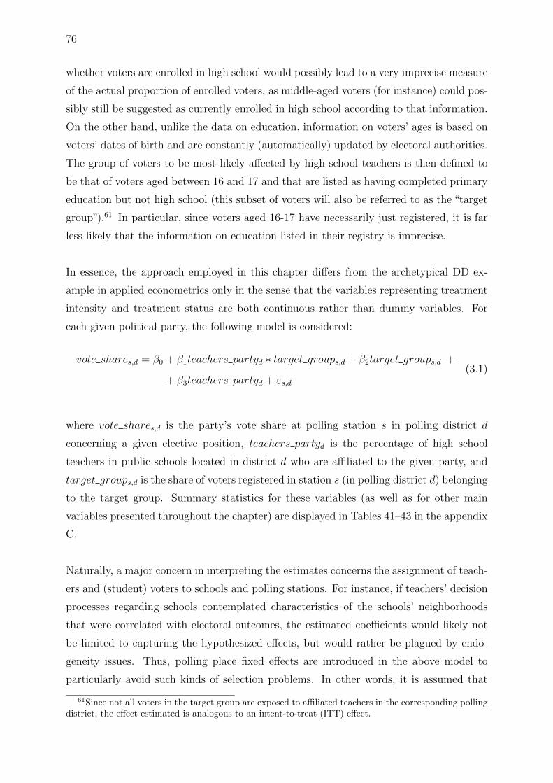
76
whether voters are enrolled in high school would possibly lead to a very imprecise measure
of the actual proportion of enrolled voters, as middle-aged voters (for instance) could pos-
sibly still be suggested as currently enrolled in high school according to that information.
On the other hand, unlike the data on education, information on voters’ ages is based on
voters’ dates of birth and are constantly (automatically) updated by electoral authorities.
The group of voters to be most likely affected by high school teachers is then defined to
be that of voters aged between 16 and 17 and that are listed as having completed primary
education but not high school (this subset of voters will also be referred to as the “target
group”).61 In particular, since voters aged 16-17 have necessarily just registered, it is far
less likely that the information on education listed in their registry is imprecise.
In essence, the approach employed in this chapter differs from the archetypical DD ex-
ample in applied econometrics only in the sense that the variables representing treatment
intensity and treatment status are both continuous rather than dummy variables. For
each given political party, the following model is considered:
vote shares,d = β0 + β1teachers partyd ∗ target groups,d + β2target groups,d +
+ β3teachers partyd + εs,d(3.1)
where vote shares,d is the party’s vote share at polling station s in polling district d
concerning a given elective position, teachers partyd is the percentage of high school
teachers in public schools located in district d who are affiliated to the given party, and
target groups,d is the share of voters registered in station s (in polling district d) belonging
to the target group. Summary statistics for these variables (as well as for other main
variables presented throughout the chapter) are displayed in Tables 41–43 in the appendix
C.
Naturally, a major concern in interpreting the estimates concerns the assignment of teach-
ers and (student) voters to schools and polling stations. For instance, if teachers’ decision
processes regarding schools contemplated characteristics of the schools’ neighborhoods
that were correlated with electoral outcomes, the estimated coefficients would likely not
be limited to capturing the hypothesized effects, but would rather be plagued by endo-
geneity issues. Thus, polling place fixed effects are introduced in the above model to
particularly avoid such kinds of selection problems. In other words, it is assumed that
61Since not all voters in the target group are exposed to affiliated teachers in the corresponding pollingdistrict, the effect estimated is analogous to an intent-to-treat (ITT) effect.

77
controlling for polling place fixed effects, teacher and voter assignment becomes (partially)
uncorrelated to political characteristics of polling station cohorts, and that β1 indeed cap-
tures the effect of the interaction between party-affiliated teachers and the segment of the
electorate that is more likely to be politically influenced by them. It is important to note
that introducing polling place fixed effects should not pose issues to the estimates as the
average number of stations within a polling place in the sample is fairly high.62
Ultimately, then, the following model is estimated:
vote shares,d = β0 + β1teachers partyd ∗ target groups,d + β2target groups,d +
+ γb + εs,d(3.2)
where γb denotes a polling place fixed effect, which in particular absorbs all kinds of
variation at the polling district level, such as that from teachers partyd. Aside from
separately estimating model (3.2) for each of the four parties listed above, the effect of
interest is also estimated by pooling the observations for these parties. In that case, the
model may be rewritten as:
vote sharep,s,d = β0 + β1teachers partyp,d ∗ target groups,d + β2target groups,d +
+ γb,p + εs,d,p
(3.3)
where vote shares,d,p is the vote share obtained by party p at polling station s in polling
district d, teachers partyd,p is the percentage of high school teachers in public schools
located in district d who are affiliated to party p, and γb,p denotes a party-polling place
fixed effect.
3.4 Main Results
To illustrate the specifications considered above, this section begins by focusing on dis-
cussing the estimates obtained for the effect of teachers affiliated to the PT on that party’s
vote share at the 2010 presidential election. The corresponding results are presented in
Table 21. Column (1) of that table presents the baseline specification of equation (3.1),
62Polling places had an average of 7.93 stations in 2008 and 8.27 stations in 2010.

78
while column (3) introduces polling place fixed effects, as described by model (3.2). Also,
column (2) considers a slight modification of model (3.2) wherein we replace polling place
fixed effects with district fixed effects.
Table 21: Effect of Teachers Affiliated to the PT on the Vote Share at the 2010Presidential Election
Dep. Variable: vote shares,d (1) (2) (3)
teachers partyd ∗ target groups,d -0.0058 0.0173*** 0.0061*(0.0112) (0.0054) (0.0033)
target groups,d 0.2610*** 0.0350** -0.0254**(0.0348) (0.0141) (0.0108)
teachers partyd 1.5683***(0.3719)
Observations 75,591 75,591 75,591R-squared 0.0480 0.6849 0.9263District FE No Yes NoPolling Place FE No No Yes
Standard errors (in parenthesis) are robust to clustering at the polling district level.*, **, and *** indicate significance at the 10%, 5% and 1% levels, respectively.
In particular, the coefficient β3, associated with teachers partyd, in column (1) shows,
as possibly expected, that the assignment of affiliated teachers across districts is highly
(and positively) correlated with the electoral performance of the corresponding party. This
research, however, is primarily interested in the signal and magnitude of the coefficient β1,
associated with the interaction between the share of affiliated high school teachers and the
share of voters in the target group. We first note that the omission of important variables
would seriously compromise inferences based on the baseline specification (model (3.1)):
while β1 is estimated to be negative (but statistically insignificant) in column (1), the
introduction of district and polling place fixed effects in columns (2) and (3), respectively,
leads to positive (and significant) estimates of that coefficient. The corresponding estimate
in column (3), for instance, indicates that once polling place specific characteristics are
accounted for, the correlation between the density of teachers affiliated to the PT and
that party’s vote share in the 2010 presidential election is stronger in polling stations
with higher shares of high school students aged between 16 and 17.
To better understand the magnitude of the estimate of β1 presented in column (3), con-
sider a polling station wherein 20% of the voters belong to the target group. Then, the
corresponding estimate indicates that an increase by one percentage point (p.p.) in the
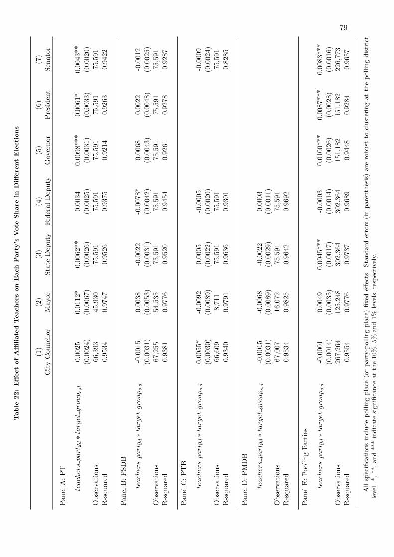
79
Table
22:
Eff
ect
of
Affi
liate
dT
each
ers
on
Each
Part
y’s
Vote
Share
inD
iffere
nt
Ele
cti
ons
(1)
(2)
(3)
(4)
(5)
(6)
(7)
Cit
yC
oun
cilo
rM
ayor
Sta
teD
eputy
Fed
eral
Dep
uty
Gov
ernor
Pre
siden
tS
enato
r
Pan
elA
:P
T
teach
ersparty d∗target
groups,d
0.0
025
0.01
12*
0.00
62**
0.003
40.
0098
***
0.0
061*
0.00
43**
(0.0
024)
(0.0
067)
(0.0
026)
(0.0
025
)(0
.0031
)(0
.003
3)(0
.0020
)O
bse
rvat
ions
66,3
9345
,930
75,5
9175,
591
75,5
91
75,
591
75,5
91
R-s
qu
ared
0.9
534
0.97
470.
9526
0.937
50.
9214
0.9
263
0.94
22
Pan
elB
:P
SD
B
teach
ersparty d∗target
groups,d
-0.0
015
0.00
38-0
.002
2-0
.0078
*0.
006
80.0
022
-0.0
012
(0.0
031)
(0.0
053)
(0.0
031)
(0.0
042
)(0
.0043
)(0
.004
8)(0
.0025
)O
bse
rvat
ions
67,2
5554
,535
75,5
9175,
591
75,5
91
75,
591
75,5
91
R-s
qu
ared
0.9
381
0.97
760.
9520
0.945
40.
9261
0.9
278
0.92
87
Pan
elC
:P
TB
teach
ersparty d∗target
groups,d
0.00
55*
-0.0
092
0.00
05-0
.0005
-0.0
009
(0.0
030)
(0.0
089)
(0.0
022)
(0.0
020
)(0
.0024
)O
bse
rvat
ions
66,6
098,
711
75,5
9175
,591
75,5
91R
-squ
ared
0.9
340
0.97
910.
9636
0.930
10.
828
5
Pan
elD
:P
MD
B
teach
ersparty d∗target
groups,d
-0.0
015
-0.0
068
-0.0
022
0.00
03(0
.003
1)(0
.008
9)(0
.002
9)(0
.0011
)O
bse
rvat
ions
67,0
0716
,072
75,5
9175,
591
R-s
qu
ared
0.9
534
0.98
250.
9642
0.969
2
Pan
elE
:P
ooling
Par
ties
teach
ersparty d∗target
groups,d
-0.0
001
0.00
490.
0045
***
-0.0
003
0.01
00**
*0.
0087
***
0.00
83**
*(0
.001
4)(0
.003
5)(0
.001
7)(0
.0014
)(0
.0026
)(0
.002
8)(0
.0016
)O
bse
rvat
ions
267,
264
125,
248
302,
364
302,
364
151
,182
151,
182
226
,773
R-s
qu
ared
0.9
554
0.97
760.
9737
0.968
90.
9448
0.9
284
0.96
57
All
spec
ifica
tion
sin
clu
de
pol
ling
pla
ce(o
rpar
ty-p
olling
pla
ce)
fixed
effec
ts.
Sta
nd
ard
erro
rs(i
npare
nth
esis
)are
robu
stto
clu
ster
ing
at
the
pollin
gdis
tric
tle
vel.
*,**
,an
d**
*in
dic
ate
sign
ifica
nce
atth
e10
%,
5%an
d1%
leve
ls,
resp
ecti
vely
.

80
share of high school teachers affiliated to the PT (in the related polling district) is associ-
ated with an increase by 0.12 p.p. in the PT’s vote share at that polling station in the 2010
presidential election as a result of their influence over voting-aged students. Were that
polling station to contain 400 voters, for instance, such an effect would correspond to an
average increase by approximately 0.5 in the number of votes received by the PT at that
station. Such a magnitude may become even more relevant upon the observation that
these estimates may be understood as intent-to-treat effects, since not all voters in the
target group are guaranteed to be exposed to affiliated teachers. In that sense, the effect
would be more important the smaller the share of voters actually exposed to affiliated
teachers.
Next, the corresponding results for the four considered political parties and for each
elective position disputed in 2008 and 2010 are presented. Such presentation, however,
is restricted to the estimates obtained upon the estimation of models (3.2) and (3.3),
wherein polling place fixed effects are included. Panels A through D of Table 22 present
the results for the PT, the PSDB, the PTB, and the PMDB, whereas Panel E of that
table shows the estimates obtained upon polling the observations of these parties. It is
important to observe from the latter panel that, aside from the positions of city councilor
and federal deputy (which are associated with negative and insignificant coefficients very
close to zero), the presence of teachers affiliated to a “generic” party is associated with a
positive effect on the vote share exhibited by such a party in all other elections. Moreover,
this seems particularly true for elective positions filled under plurality rules – i.e. mayor,
governor, president, and senator – for which the magnitude of the coefficients is higher
(although the estimate corresponding to the position of mayor is statistically insignificant).
The larger effect in Panel E is found for the position of governor, and indicates that in
a polling station wherein 20% of the voters belong to the target group, a share of 1% of
teachers affiliated to a party is responsible for 0.2 p.p. of the corresponding vote share as
a result of the interaction with voting-aged high school students.
The contrast between the magnitude of the estimates obtained for elections under plurality
rules and those for elections under a proportional representation system goes in line with
the possibility that teachers opt to configure their propaganda in order to praise not their
party as a whole, but rather the figure of specific candidates. Arguably, this kind of
behavior would surely be harder in the occasions where multiple candidates from a single
party could run for the same office, such as elections under proportional representation
systems (but not those under plurality rules).
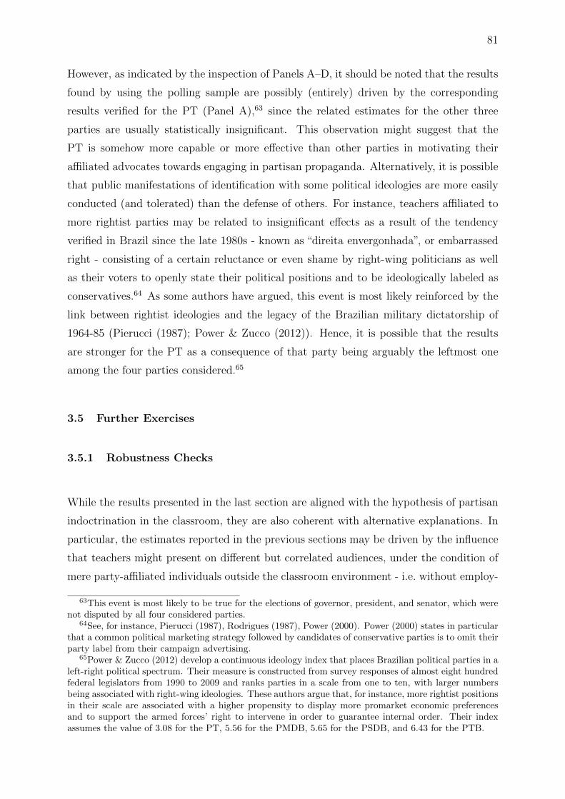
81
However, as indicated by the inspection of Panels A–D, it should be noted that the results
found by using the polling sample are possibly (entirely) driven by the corresponding
results verified for the PT (Panel A),63 since the related estimates for the other three
parties are usually statistically insignificant. This observation might suggest that the
PT is somehow more capable or more effective than other parties in motivating their
affiliated advocates towards engaging in partisan propaganda. Alternatively, it is possible
that public manifestations of identification with some political ideologies are more easily
conducted (and tolerated) than the defense of others. For instance, teachers affiliated to
more rightist parties may be related to insignificant effects as a result of the tendency
verified in Brazil since the late 1980s - known as “direita envergonhada”, or embarrassed
right - consisting of a certain reluctance or even shame by right-wing politicians as well
as their voters to openly state their political positions and to be ideologically labeled as
conservatives.64 As some authors have argued, this event is most likely reinforced by the
link between rightist ideologies and the legacy of the Brazilian military dictatorship of
1964-85 (Pierucci (1987); Power & Zucco (2012)). Hence, it is possible that the results
are stronger for the PT as a consequence of that party being arguably the leftmost one
among the four parties considered.65
3.5 Further Exercises
3.5.1 Robustness Checks
While the results presented in the last section are aligned with the hypothesis of partisan
indoctrination in the classroom, they are also coherent with alternative explanations. In
particular, the estimates reported in the previous sections may be driven by the influence
that teachers might present on different but correlated audiences, under the condition of
mere party-affiliated individuals outside the classroom environment - i.e. without employ-
63This event is most likely to be true for the elections of governor, president, and senator, which werenot disputed by all four considered parties.
64See, for instance, Pierucci (1987), Rodrigues (1987), Power (2000). Power (2000) states in particularthat a common political marketing strategy followed by candidates of conservative parties is to omit theirparty label from their campaign advertising.
65Power & Zucco (2012) develop a continuous ideology index that places Brazilian political parties in aleft-right political spectrum. Their measure is constructed from survey responses of almost eight hundredfederal legislators from 1990 to 2009 and ranks parties in a scale from one to ten, with larger numbersbeing associated with right-wing ideologies. These authors argue that, for instance, more rightist positionsin their scale are associated with a higher propensity to display more promarket economic preferencesand to support the armed forces’ right to intervene in order to guarantee internal order. Their indexassumes the value of 3.08 for the PT, 5.56 for the PMDB, 5.65 for the PSDB, and 6.43 for the PTB.

82
ing their teacher status to broaden their audience - and thus be affected by an omitted
variable problem.
In order to explore whether this is the case, a similar exercise to that presented above,
consisting of replacing the target group with a demographic group that is far less likely to
interact with high school teachers (at least in a teacher-pupil relationship), is conducted.
Namely, it is considered voters aged 16–17 that either had not initiated basic education,
or that had already completed high school at the time of electoral registration (this group
will henceforth be referred to as the “placebo group”). Specifically, models (3.2) and (3.3)
are reestimated after replacing target groups,d with the share of voters in station s (in
polling district d) belonging to that placebo group (denoted placebo groups,d).
The particular choice for voters aged 16–17 is made for two main reasons. First, as
previously stated, considering such an age cohort allows to avoid imprecisions in voters’
actual educational status at the time of election, as the corresponding voters are likely
to have just registered for voting. Thus, voters aged 16–17 that are indicated by their
electoral registers not to be enrolled in high school are expected to effectively be in that
situation at the time of election. Also, should the previous estimates be driven by affiliated
teachers influencing all voters aged 16–17 alike—i.e. regardless of being their high school
students—one should expect to find estimates of a similar impact of those teachers on
voting patterns of the placebo group. On the other hand, the absence of significant effects
in that case could serve as further indication that the previously found evidence is indeed
related to intraclassroom interactions between affiliated teachers and their pupils.
The corresponding results of that exercise are presented in Table 23. The estimates
related to the PT and to the sample that pools the four considered parties (Panels A and
E) are overall statistically insignificant, with the exception of the coefficients regarding
the presidential election. Since these panels were the ones for which significant estimates
were found in the main results, further confidence is gained on the hypothesis of political
indoctrination in the classroom. The same event (of statistical insignificance) applies to
the coefficients related to the PTB (Panel C) and to the PMDB (Panel D). On the other
hand, some statistically significant estimates are found regarding the electoral influence
of teachers affiliated to the PSDB on the placebo group.
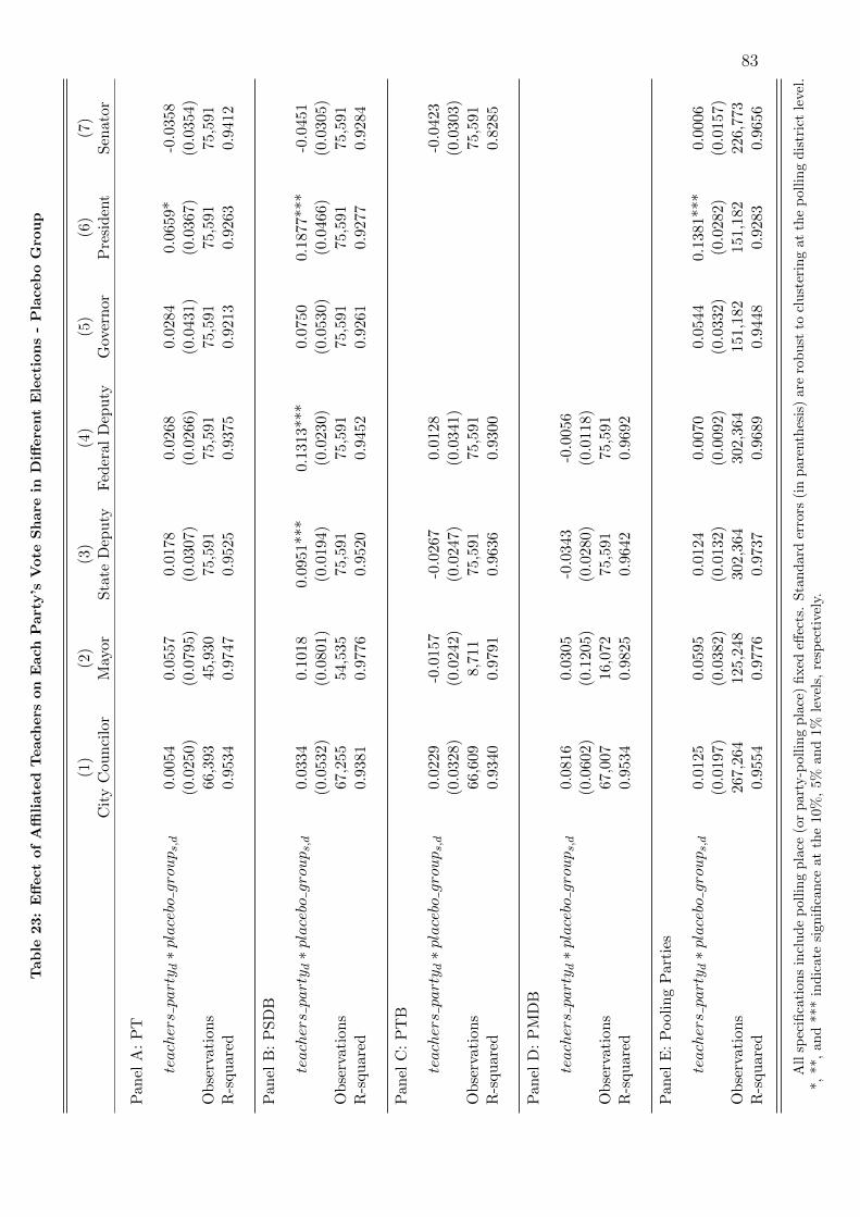
83
Table
23:
Eff
ect
of
Affi
liate
dT
each
ers
on
Each
Part
y’s
Vote
Share
inD
iffere
nt
Ele
cti
ons
-P
laceb
oG
roup
(1)
(2)
(3)
(4)
(5)
(6)
(7)
Cit
yC
oun
cilo
rM
ayor
Sta
teD
eputy
Fed
eral
Dep
uty
Gov
ernor
Pre
sid
ent
Sen
ato
r
Pan
elA
:P
T
teach
ersparty d∗placebo
groups,d
0.0
054
0.05
570.
0178
0.026
80.
0284
0.06
59*
-0.0
358
(0.0
250)
(0.0
795)
(0.0
307)
(0.0
266
)(0
.0431
)(0
.036
7)(0
.0354
)O
bse
rvat
ions
66,3
93
45,9
3075
,591
75,
591
75,5
9175,
591
75,5
91R
-squ
ared
0.95
340.
9747
0.95
250.9
375
0.92
130.9
263
0.94
12
Pan
elB
:P
SD
B
teach
ersparty d∗placebo
groups,d
0.0
334
0.10
180.
0951
***
0.131
3***
0.07
500.
1877
***
-0.0
451
(0.0
532)
(0.0
801)
(0.0
194)
(0.0
230
)(0
.0530
)(0
.046
6)(0
.0305
)O
bse
rvat
ions
67,2
55
54,5
3575
,591
75,
591
75,5
9175,
591
75,5
91R
-squ
ared
0.93
810.
9776
0.95
200.9
452
0.92
610.9
277
0.92
84
Pan
elC
:P
TB
teach
ersparty d∗placebo
groups,d
0.0
229
-0.0
157
-0.0
267
0.0
128
-0.0
423
(0.0
328)
(0.0
242)
(0.0
247)
(0.0
341
)(0
.0303
)O
bse
rvat
ions
66,6
09
8,71
175
,591
75,
591
75,
591
R-s
qu
ared
0.93
400.
9791
0.96
360.9
300
0.82
85
Pan
elD
:P
MD
B
teach
ersparty d∗placebo
groups,d
0.0
816
0.03
05-0
.034
3-0
.0056
(0.0
602)
(0.1
205)
(0.0
280)
(0.0
118
)O
bse
rvat
ions
67,0
07
16,0
7275
,591
75,
591
R-s
qu
ared
0.95
340.
9825
0.96
420.9
692
Pan
elE
:P
ooling
Par
ties
teach
ersparty d∗placebo
groups,d
0.0
125
0.05
950.
0124
0.007
00.
0544
0.13
81**
*0.0
006
(0.0
197)
(0.0
382)
(0.0
132)
(0.0
092
)(0
.0332
)(0
.028
2)(0
.0157
)O
bse
rvat
ions
267,
264
125,
248
302,
364
302,
364
151
,182
151,
182
226
,773
R-s
qu
ared
0.95
540.
9776
0.97
370.9
689
0.94
480.9
283
0.96
56
All
spec
ifica
tion
sin
clu
de
pol
lin
gpla
ce(o
rpar
ty-p
ollin
gpla
ce)
fixed
effec
ts.
Sta
ndard
erro
rs(i
np
are
nth
esis
)are
robust
tocl
ust
erin
gat
the
pollin
gd
istr
ict
leve
l.*,
**,
and
***
indic
ate
sign
ifica
nce
atth
e10
%,
5%an
d1%
leve
ls,
resp
ecti
vely
.
84
3.5.2 Effects on Turnout
Next, it is exploited whether affiliated teachers have an impact on their pupils’ electoral
turnout. In other words, this section tests whether the positive influence – evidenced in
Section 3.4 – of such teachers on parties’ vote shares specifically consists in convincing
students that would otherwise not vote. In particular, confronting that hypothesis with
the alternative possibility that the effect of affiliated teachers on vote shares is actually
driven by shifting students’ political preferences from one party to another could lead to
a better understanding of the effectiveness of political indoctrination by teachers as well
as of political participation among the young, for instance.
For each of the four considered parties and for each election year, the following model is
estimated:
turnouts,d = β0 + β1teachers partyd ∗ target groups,d + β2target groups,d +
+ γb + εs,d(3.4)
where turnouts,d denotes the turnout rate (ranging from 0 to 100) at polling station
s in polling district d. Unlike the preceding regressions, however, in estimating model
(3.4) observations on all polling stations (at the given election year) are used rather than
only those on stations in administrative units (municipalities) wherein the given party
effectively ran for election (and had a well defined vote share). As before, model (3.4)
is also estimated by pooling observations on the four parties after replacing polling place
fixed effects with party-polling place fixed effects.
The corresponding results are presented in Table 24. Panel A of that table presents
estimates regarding the effect on turnout at the 2008 local elections, whereas Panel B
considers turnout at the 2010 general elections. First, it is possible to observe from Panel
A that the density of teachers affiliated to the PSDB or to the PTB has a positive effect
(as a result of their interactions with voting-aged students) on turnout at local elections.
For instance, the coefficient associated with the PTB indicates that, regarding a polling
station wherein 20% of the voters belong to the target group, a share of 1 p.p. of teachers
affiliated to that party is responsible for almost 0.3 p.p. of the turnout rate at such a
polling station in 2008. However, as previously shown in Table 22, such an effect on
turnout was not (significantly) translated into positive effects on these two parties’ vote

85
shares in the corresponding elections. Similarly, despite having presented a significant
impact on vote shares, teacher affiliation to the PT is not suggested to influence student
turnout. Thus, for that party it may be the case that affiliated teachers are actually
able to change the political leanings of students that would vote for another party. On
the other hand, the estimates associated with turnout at the 2010 general elections are
overall statistically insignificant. An exception is made for the coefficient related to the
PMDB, which is negative and significant at the 10% level. We conjecture, though, that
the significance of that coefficient may be related to the fact that there was no candidate
running under the PMDB for the positions of governor, senator, or president in 2010.
Table 24: Effect of Affiliated Teachers on Voter Turnout
(1) (2) (3) (4) (5)PT PSDB PTB PMDB Pooling
Panel A: 2008 Local Elections
teachers partyd ∗ target groups,d -0.0036 0.0087** 0.0144** 0.0002 0.0033*(0.0038) (0.0036) (0.0058) (0.0048) (0.0019)
Observations 67,355 67,355 67,355 67,355 269,420R-squared 0.6866 0.6867 0.6867 0.6866 0.6866
Panel B: 2010 General Elections
teachers partyd ∗ target groups,d -0.0059 -0.0060 -0.0100 -0.0092* -0.0065**(0.0052) (0.0062) (0.0079) (0.0050) (0.0028)
Observations 75,591 75,591 75,591 75,591 302,364R-squared 0.6608 0.6608 0.6608 0.6608 0.6608
All specifications include polling place (or party-polling place) fixed effects. Standard errors (in parenthe-sis) are robust to clustering at the polling district level. *, **, and *** indicate significance at the 10%, 5%and 1% levels, respectively.
3.6 Conclusion
This paper investigated the influence that politically active teachers may present in the
electoral process through shaping their students’ voting behavior by means of partisan
propaganda in the classroom environment. This analysis is achieved by exploiting very
rich databases on public high school teachers and on party-affiliated voters - through which
it was possible to identify high school teachers’ political affiliations - and by considering
the relationship between the density of affiliated teachers and electoral outcomes for the
corresponding party in a given region.
86
To overcome the matter of selection in the assignment of teachers to schools and of voters
to polling places (which would likely bias the estimates), it was exploited variation in
the intensity of the hypothesized effect according to characteristics of the electorate at a
level (polling stations) into which, arguably, neither teachers nor voters are able to select
themselves.
Evidence consistent with the hypothesis of political indoctrination in the classroom was
found. Moreover, the effect of the presence of party-affiliated teachers on a party’s vote
share seems to be more pronounced for elections based on plurality voting systems. How-
ever, it was found evidence that such an effect is apparently driven by teachers affiliated
to the Workers’ Party. In addition, such teachers do not appear to have an effect on elec-
toral turnout by their students, so their impact on vote shares is suggested to take place
through altering the political leanings of students that would turn out to vote regardless
of their interference.
The findings indicating party-affiliated teachers may play such a role raise very important
questions, especially regarding what kind of teaching is ultimately being performed in
their classes, and whether the suggested diversion from curriculum content standards is
deleterious to educational outcomes of their students. In this sense, it would be worthwhile
to also investigate whether teachers of certain subjects have relatively more leeway to
define their courses’ contents (and their ways of presenting them), and thus a greater
ability to influence electoral outcomes. Moreover, another interesting topic concerns the
reasons why teachers would be engaging in that kind of behavior, and particularly whether
party-affiliated teachers are being paid to politically influence their pupils. Such questions
are left as agenda for future research.

87

88

89
BIBLIOGRAPHY
ACEMOGLU, D.; JOHNSON, S.; ROBINSON, J. A. Reversal of fortune: Geographyand institutions in the making of the modern world income distribution. The QuarterlyJournal of Economics, v. 117, n. 4, p. 1231–1294, November 2002. Disponıvel em: <http://ideas.repec.org/a/tpr/qjecon/v117y2002i4p1231-1294.html>.
ACEMOGLU, D.; ROBINSON, J. A. Persistence of power, elites, and institutions. Amer-ican Economic Review, v. 98, n. 1, p. 267–93, March 2008.
ACEMOGLU, D.; ROBINSON, J. A.; SANTOS, R. J. The monopoly of violence: Evi-dence from colombia. Journal of the European Economic Association, Blackwell Publish-ing Inc, v. 11, p. 5–44, 2013. ISSN 1542-4774. Disponıvel em: <http://dx.doi.org/10.1111/j.1542-4774.2012.01099.x>.
ALESINA, A.; TABELLINI, G. Bureaucrats or politicians? part i: A single policy task.American Economic Review, v. 97, n. 1, p. 169–179, 2007. Disponıvel em: <http://www.aeaweb.org/articles.php?doi=10.1257/aer.97.1.169>.
ALMEIDA, M. L. de. Comunicacao de massa no Brasil. [S.l.]: EdicoesJupiter;[distribuidor: Cultura Representacoes], 1971.
ARAUJO, M. C. et al. Local inequality and project choice: Theory and evidence fromecuador. Journal of Public Economics, Elsevier, v. 92, n. 5, p. 1022–1046, 2008.
ARULAMPALAM, W. et al. Electoral goals and center-state transfers: A theoreticalmodel and empirical evidence from india. Journal of Development Economics, Elsevier,v. 88, n. 1, p. 103–119, 2009.
BARDHAN, P.; MOOKHERJEE, D. Capture and governance at local and national levels.American Economic Review, JSTOR, p. 135–139, 2000.
BESLEY, T.; BURGESS, R. The political economy of government responsiveness: Theoryand evidence from india. The Quarterly Journal of Economics, v. 117, n. 4, p. 1415–1451,2002. Disponıvel em: <http://qje.oxfordjournals.org/content/117/4/1415.abstract>.
BESLEY, T.; COATE, S. Elected versus appointed regulators: Theory and evi-dence. Journal of the European Economic Association, Blackwell Publishing Ltd, v. 1,n. 5, p. 1176–1206, 2003. ISSN 1542-4774. Disponıvel em: <http://dx.doi.org/10.1162/154247603770383424>.
BESLEY, T.; PRAT, A. Handcuffs for the grabbing hand? the role of the media inpolitical accountability. American Economic Review, Citeseer, v. 96, n. 3, p. 720–736,2006.
BO, E. D.; TELLA, R. D. Capture by threat. Journal of Political Economy, v. 111,n. 5, p. 1123–1152, October 2003. Disponıvel em: <http://ideas.repec.org/a/ucp/jpolec/v111y2003i5p1123-1152.html>.
BROLLO, F.; NANNICINI, T. Tying your enemy’s hands in close races: The politicsof federal transfers in brazil. American Political Science Review, Cambridge Univ Press,v. 106, n. 04, p. 742–761, 2012.
90
CARD, D. Using regional variation in wages to measure the effects of the federal minimumwage. Industrial and Labor Relations Review, v. 46, n. 1, p. 22–37, 1992.
CASTRO, A. B. d.; SOUZA, F. P. d. A economia brasileira em marcha forcada. 3. ed.[S.l.]: Paz e Terra, 2004.
CASTRO, L. B. d. Esperanca, frustracao e aprendizado: a historia da nova republica. In:GIAMBIAGI, F.; VILLELA, A. (Ed.). Economia Brasileira Contemporanea: 1945-2004.[S.l.]: Elsevier, 2005.
CHONG, A.; FERRARA, E. L. Television and divorce: Evidence from brazilian novelas.Journal of the European Economic Association, Wiley Online Library, v. 7, n. 2-3, p.458–468, 2009.
CORRALES, J. Political obstacles to expanding and improving schooling in developingcountries. Educating all children: A global agenda, MIT Press, p. 231–299, 2006.
DEE, T. S. Are there civic returns to education? Journal of Public Economics, Elsevier,v. 88, n. 9, p. 1697–1720, 2004.
DELLAVIGNA, S.; KAPLAN, E. The Fox News effect: Media bias and voting. [S.l.], 2006.
DJANKOV, S. et al. Who owns the media? [S.l.], 2001.
DUFLO, E. Schooling and labor market consequences of school construction in indonesia:Evidence from an unusual policy experiment. American Economic Review, v. 91, n. 4,p. 795, 2001.
DYCK, A.; ZINGALES, L. The right to tell: the role of the media in development, chap.The corporate governance role of the media. The World Bank, 2002.
EBERTS, R. W.; STONE, J. A. Teacher unions and the productivity of public schools.Industrial and Labor Relations Review, Sage Publications, Inc., v. 40, n. 3, p. pp. 354–363,1987. ISSN 00197939. Disponıvel em: <http://www.jstor.org/stable/2523492>.
FARIA, V.; POTTER, J. Television, Telenovelas, and Fertility Change in North-EastBrazil” a Richard Leete,(ed.) Dynamic of Values in Fertility Change, Nueva York: IUSSP.[S.l.]: Oxford University Press, 1999.
FERRARA, E. L.; CHONG, A.; DURYEA, S. Soap operas and fertility: Evidence frombrazil. American Economic Journal: Applied Economics, JSTOR, p. 1–31, 2012.
FINAN, F. Political patronage and local development: A brazilian case study. ARE, UCBerkeley, 2004.
GALASSO, E.; RAVALLION, M. Decentralized targeting of an antipoverty program.Journal of Public economics, Elsevier, v. 89, n. 4, p. 705–727, 2005.
GENTZKOW, M. Television and voter turnout. The Quarterly Journal of Economics,JSTOR, p. 931–972, 2006.
GENTZKOW, M.; GLAESER, E. L.; GOLDIN, C. The rise of the fourth estate. how news-papers became informative and why it mattered. In: Corruption and Reform: Lessonsfrom America’s Economic History. [S.l.]: University of Chicago Press, 2006. p. 187–230.

91
GEORGE, L.; WALDFOGEL, J. Does the new york times spread ignorance and apathy?American Economic Review, forthcoming, 2002.
GERBER, A.; KARLAN, D. S.; BERGAN, D. Does the media matter? a field experimentmeasuring the effect of newspapers on voting behavior and political opinions. A FieldExperiment Measuring the Effect of Newspapers on Voting Behavior and Political Opinions(February 15, 2006). Yale Economic Applications and Policy Discussion Paper, n. 12,2006.
GERBER, A. S.; GREEN, D. P. The effects of canvassing, telephone calls, and direct mailon voter turnout: A field experiment. American Political Science Review, Cambridge UnivPress, v. 94, n. 03, p. 653–663, 2000.
GINSBURG, M. B. et al. Educators/politics. Comparative education review, JSTOR, p.417–445, 1992.
GROSECLOSE, T.; MILYO, J. A measure of media bias. The Quarterly Journal of Eco-nomics, JSTOR, p. 1191–1237, 2005.
HAHN, C. Becoming political: Comparative perspectives on citizenship education. [S.l.]:Suny Press, 1998.
HAMILTON, J. All the news that’s fit to sell: How the market transforms informationinto news. [S.l.]: Princeton University Press, 2004.
HANUSHEK, E. Publicly provided education. in: Auerbach, a., feldstein, m. (eds.), thehandbook of public economics, volume 4, elsevier, amsterdam. p. 2045–2141, 2002.
HERMAN, E. S.; CHOMSKY, N. Manufacturing consent: The political economy of themass media. [S.l.]: Random House, 2010.
HERMAN, J. Reformas, endividamento e o ”milagre” economico. In: GIAMBIAGI, F.;VILLELA, A. (Ed.). Economia Brasileira Contemporanea: 1945-2004. [S.l.]: Elsevier,2005.
HILLYGUS, D. S. The missing link: Exploring the relationship between higher educationand political engagement. Political Behavior, Springer, v. 27, n. 1, p. 25–47, 2005.
HOROWITZ, D. The professors: The 101 most dangerous academics in America. [S.l.]:Regnery Publishing, 2006.
HOXBY, C. M. How teachers’ unions affect education production. The Quarterly Journalof Economics, v. 111, n. 3, p. 671–718, 1996. Disponıvel em: <http://qje.oxfordjournals.org/content/111/3/671.abstract>.
IMBENS, G. W.; LEMIEUX, T. Regression discontinuity designs: A guide to prac-tice. Journal of Econometrics, v. 142, n. 2, p. 615 – 635, 2008. ISSN 0304-4076.The regression discontinuity design: Theory and applications. Disponıvel em: <http://www.sciencedirect.com/science/article/pii/S0304407607001091>.
KAM, C. D.; PALMER, C. L. Reconsidering the effects of education on political partici-pation. The Journal of Politics, Cambridge Univ Press, v. 70, n. 03, p. 612–631, 2008.
92
KAM, C. D.; PALMER, C. L. Reconsidering the effects of education on political partici-pation. The Journal of Politics, v. 70, p. 612–631, 7 2008. ISSN 1468-2508.
KEEFER, P. Clientelism, credibility, and the policy choices of young democracies. Amer-ican Journal of Political Science, Blackwell Publishing Inc, v. 51, n. 4, p. 804–821, 2007.ISSN 1540-5907. Disponıvel em: <http://dx.doi.org/10.1111/j.1540-5907.2007.00282.x>.
KEELE, L.; TITIUNIK, R.; ZUBIZARRETA, J. R. Enhancing a geographic regressiondiscontinuity design through matching to estimate the effect of ballot initiatives on voterturnout. Journal of the Royal Statistical Society: Series A (Statistics in Society), v. 178,n. 1, p. 223–239, 2015. ISSN 1467-985X. Disponıvel em: <http://dx.doi.org/10.1111/rssa.12056>.
KHEMANI, S. Does delegation of fiscal policy to an independent agency make a dif-ference? evidence from intergovernmental transfers in india. Journal of DevelopmentEconomics, Elsevier, v. 82, n. 2, p. 464–484, 2007.
KITSCHELT, H.; WILKINSON, S. I. Patrons, clients and policies: Patterns of democraticaccountability and political competition. [S.l.]: Cambridge University Press, 2007.
LARREGUY, H. Monitoring political brokers: Evidence from clientelistic networks inmexico. 2013.
LARREGUY, H.; MARSHALL, J.; SNYDER, J. M. Political advertising in consolidatingdemocracies: Locally dominant parties and the equalization of media access in mexico.APSA 2014 Annual Meeting Paper, 2014. Disponıvel em: <http://ssrn.com/abstract=2454757>.
LEaO, S. Essays on Banking. Tese (Doutorado) — Pontifıcia Universidade Catolica doRio de Janeiro, 2011.
LIMA, V. A. d. Comunicacao e polıtica. Sao Paulo: Hacker Editores, 2001.
LIMONGI, F.; CHEIDUB, J. A.; FIGUEIREDO, A. C. Participacao polıtica no brasil.In: ARRETCHE, M. (Ed.). Trajetorias das Desigualdades: Como o Brasil Mudou nosUltimos Cinquenta Anos. [S.l.]: Editora Unesp, 2015.
MAINWARING, S. Rethinking party systems in the third wave of democratization: thecase of Brazil. [S.l.]: Stanford University Press, 1999.
MARTINEZ-BRAVO, M. The role of local officials in new democracies: Evidence fromindonesia. American Economic Review, v. 104, n. 4, p. 1244–87, 2014. Disponıvel em:<http://www.aeaweb.org/articles.php?doi=10.1257/aer.104.4.1244>.
MARTINEZ-BRAVO, M.; MUKHERJEE, P. An empirical investigation of the legaciesof non-democratic regimes: The case of soeharto’s mayors in indonesia. Working paper,2015.
MARTINEZ-BRAVO, M. et al. Do local elections in non-democracies increase account-ability? Evidence from rural China. [S.l.], 2011.
MATTOS, S. A. S. Domestic and foreign advertising in television and mass media growth:a case study of Brazil. Tese (Doutorado) — University of Texas at Austin, 1982.

93
MCMILLAN, J.; ZOIDO, P. How to subvert democracy: Montesinos in peru. CEPRDiscussion Paper, 2004.
MIGUEL, L. F. Meios de comunicacao de massa e polıtica no brasil. Dialogos latinoamer-icanos, Aarhus Universitet, v. 3, p. 43–70, 2001.
MILLIGAN, K.; MORETTI, E.; OREOPOULOS, P. Does education improve citizenship?evidence from the united states and the united kingdom. Journal of Public Economics,Elsevier, v. 88, n. 9, p. 1667–1695, 2004.
MOE, T. M. Special Interest: Teachers Unions and America’s Public Schools. [S.l.]:Brookings Institution Press, 2011. ISBN 0815722729.
MYERS, J. P. Citizenship education practices of politically active teachers in porto alegre,brazil and toronto, canada. Comparative Education Review, JSTOR, v. 51, n. 1, p. 1–24,2007.
NICOLAU, J. Eleicoes No Brasi: do Imperio aos Dias Atuais. [S.l.]: Zahar, 2012.
NIE, N.; JUNN, J.; STEHLIK-BARRY, K. Education and citizenship in America. [S.l.]:Chicago: Cambridge University Press, 1996.
PERSSON, M. Testing the relationship between education and political participationusing the 1970 british cohort study. Political Behavior, Springer, p. 1–21, 2014.
PIERUCCI, A. F. As bases da nova direita. Novos Estudos Cebrap, v. 19, p. 26–45, 1987.
PORTO, M. P. Telenovelas and national identity in brazil. In: IX International Congressof the Brazilian Studies Association (BRASA), New Orleans. [S.l.: s.n.], 2008.
POWER, T. J. The Political Right in Postauthoritarian Brazil: Elites, Institutions, andDemocratization. [S.l.]: University Park: Pennsylvania State University Press, 2000.
POWER, T. J.; ZUCCO, C. Elite preferences in a consolidating democracy: the brazilianlegislative surveys, 1990–2009. Latin American Politics and Society, Wiley Online Library,v. 54, n. 4, p. 1–27, 2012.
PRAT, A.; STROMBERG, D. The political economy of mass media. CEPR DiscussionPaper No. DP8246, 2011.
PRIOR, M. Post-broadcast democracy: How media choice increases inequality in politicalinvolvement and polarizes elections. [S.l.]: Cambridge University Press, 2007.
PUGLISI, R. Being the new york times: the political behaviour of a newspaper. The BEJournal of Economic Analysis & Policy, v. 11, n. 1, 2011.
ROCKOFF, J. E. The impact of individual teachers on student achievement: Evidencefrom panel data. American Economic Review, JSTOR, p. 247–252, 2004.
RODRIGUES, L. M. Quem e quem na Constituinte: uma analise socio-polıtica dos par-tidos e deputados. [S.l.]: OESP, 1987.
SCHAFFER, F. C. Elections for sale: the causes and consequences of vote buying. [S.l.]:Lynne Rienner Publishers Londres, 2007.

94
SCHUGURENSKY, D.; MYERS, J. A framework to explore lifelong learning: The case ofthe civic education of civics teachers. International Journal of Lifelong Education, Taylor& Francis, v. 22, n. 4, p. 325–352, 2003.
SINGER, P. O processo economico. In: DANIEL, A. R. (Ed.). Modernizacao, Ditadura eDemocracia: 1964-2012-. 1. ed. [S.l.]: Objetiva, 2014. v. 5, p. 320.
SOLE-OLLE, A.; SORRIBAS-NAVARRO, P. The effects of partisan alignment on theallocation of intergovernmental transfers. differences-in-differences estimates for spain.Journal of Public Economics, Elsevier, v. 92, n. 12, p. 2302–2319, 2008.
SOLIS, A. Does higher education cause political participation? Evidence from a regressiondiscontinuity design. [S.l.], 2013.
STRAUBHAAR, J. D. The reflection of the brazilian political opening in the telen-ovela [soap opera], 1974-1985. Studies in Latin American Popular Culture, STUDIESLATIN AMER POPULAR CULTURE C/O CHARLES TATUM, CO-EDITOR, UNIVARIZONA, FACULTY HUMANITIES, TUCSON, AZ 85721, v. 7, p. 59–76, 1988.
STRAUBHAAR, J. D. Television and video in the transition from military to civilian rulein brazil. Latin American Research Review, JSTOR, p. 140–154, 1989.
STROMBERG, D. Radio’s impact on public spending. The Quarterly Journal of Eco-nomics, JSTOR, p. 189–221, 2004.
TELLA, R. D.; FRANCESCHELLI, I. Government advertising and media coverage ofcorruption scandals. [S.l.], 2009.
WESTHEIMER, J.; KAHNE, J. What kind of citizen? political choices and educationalgoals. Encounters on education, v. 4, 2008.
WOLFINGER, R. E.; ROSENSTONE, S. J. Who votes? [S.l.]: New Haven: Yale Uni-versity Press, 1980.

95
Appendix A
Figure 11: Municipalities with appointed mayors in the sample and neighbors used as thecontrol group (without matching)
Table 25: Balance check of the baseline characteristics between municipalities with ap-pointed mayors and the control group (without matching)
(1) (2) (3)Mun. with
appointed mayorsControl
municipalitiesp-value
Inequality (Theil index) 38.04 36.54 0.28Share of pop. living in urban areas 32.69 31.34 0.62log(population) 9.98 9.55 0.00
Population density (inhabitants/km2) 65.24 117.33 0.49
Share of illiteracy 29.65 33.81 0.03Average years of schooling 2.15 1.84 0.01Income per capita (in minimum wages) 0.49 0.45 0.32Log(number of households) 8.27 7.86 0.00Life expectancy 54.07 53.04 0.05Share of pop. occupied 32.70 31.39 0.06Share of households with sanitation 8.91 7.87 0.59Share of households with piped water 22.98 21.37 0.58Share of households with electricity 31.48 31.38 0.98Share of pop. living in poverty 73.70 76.16 0.29
Number of municipalities 81 197

96
Table 26: Effect on the Theil index (without matching)
Dependent variable: Theil index in year t; covariates measured in t=1970
t=1980 t=1991(1) (2) (3) (4)
Appointed mayor 3.5216∗∗ 2.2897 5.6973∗∗∗ 3.7464∗∗
(1.5104) (1.4551) (1.7448) (1.6491)Inequality (Theil index) 0.5810∗∗∗ 0.5965∗∗∗ 0.2439∗∗∗ 0.3033∗∗∗
(0.0695) (0.0959) (0.0809) (0.1079)Share of pop. living in urban areas -0.0042 -0.0361
(0.0606) (0.0780)Log(population) -10.9123 23.4167∗∗
(11.0938) (11.2136)Population density -0.0016 -0.0009
(0.0010) (0.0007)Share of illiteracy -0.1758 0.1183
(0.1198) (0.1278)Average years of schooling -1.9276 4.5600∗
(2.4069) (2.3955)Income per capita (in minimum wages) 1.1827 9.1653
(6.5794) (5.9550)Log(number of households) 12.2541 -22.2124∗∗
(11.1329) (11.1984)Life expectancy 0.7802∗∗∗ 0.8159∗∗∗
(0.2714) (0.2785)Share of pop. occupied -21.4805 -35.8878∗∗
(14.9620) (17.4987)Share of households with sanitation 0.0879 0.0425
(0.0691) (0.0785)Share of households with piped water 0.0049 -0.0330
(0.0707) (0.0831)Share of households with electricity -0.1956∗∗ -0.1042
(0.0984) (0.0870)Share of pop. in poverty 0.0166 0.2216∗
(0.1663) (0.1254)
Observations 278 278 278 278R-squared 0.22 0.35 0.07 0.26
Robust standard errors in parentheses: ∗ p < 0.10, ∗∗ p < 0.05, ∗∗∗ p < 0.01
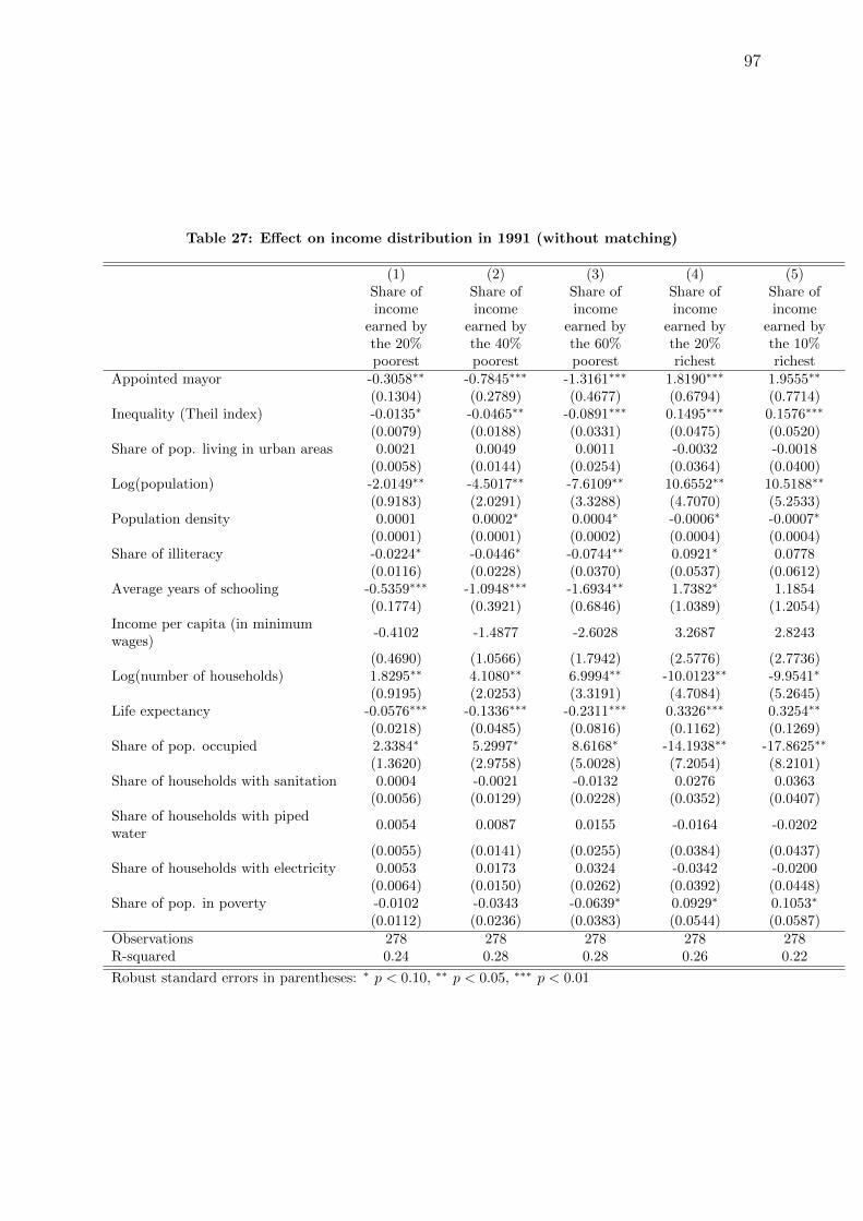
97
Table 27: Effect on income distribution in 1991 (without matching)
(1) (2) (3) (4) (5)Share ofincome
earned bythe 20%poorest
Share ofincome
earned bythe 40%poorest
Share ofincome
earned bythe 60%poorest
Share ofincome
earned bythe 20%richest
Share ofincome
earned bythe 10%richest
Appointed mayor -0.3058∗∗ -0.7845∗∗∗ -1.3161∗∗∗ 1.8190∗∗∗ 1.9555∗∗
(0.1304) (0.2789) (0.4677) (0.6794) (0.7714)Inequality (Theil index) -0.0135∗ -0.0465∗∗ -0.0891∗∗∗ 0.1495∗∗∗ 0.1576∗∗∗
(0.0079) (0.0188) (0.0331) (0.0475) (0.0520)Share of pop. living in urban areas 0.0021 0.0049 0.0011 -0.0032 -0.0018
(0.0058) (0.0144) (0.0254) (0.0364) (0.0400)Log(population) -2.0149∗∗ -4.5017∗∗ -7.6109∗∗ 10.6552∗∗ 10.5188∗∗
(0.9183) (2.0291) (3.3288) (4.7070) (5.2533)Population density 0.0001 0.0002∗ 0.0004∗ -0.0006∗ -0.0007∗
(0.0001) (0.0001) (0.0002) (0.0004) (0.0004)Share of illiteracy -0.0224∗ -0.0446∗ -0.0744∗∗ 0.0921∗ 0.0778
(0.0116) (0.0228) (0.0370) (0.0537) (0.0612)Average years of schooling -0.5359∗∗∗ -1.0948∗∗∗ -1.6934∗∗ 1.7382∗ 1.1854
(0.1774) (0.3921) (0.6846) (1.0389) (1.2054)Income per capita (in minimumwages)
-0.4102 -1.4877 -2.6028 3.2687 2.8243
(0.4690) (1.0566) (1.7942) (2.5776) (2.7736)Log(number of households) 1.8295∗∗ 4.1080∗∗ 6.9994∗∗ -10.0123∗∗ -9.9541∗
(0.9195) (2.0253) (3.3191) (4.7084) (5.2645)Life expectancy -0.0576∗∗∗ -0.1336∗∗∗ -0.2311∗∗∗ 0.3326∗∗∗ 0.3254∗∗
(0.0218) (0.0485) (0.0816) (0.1162) (0.1269)Share of pop. occupied 2.3384∗ 5.2997∗ 8.6168∗ -14.1938∗∗ -17.8625∗∗
(1.3620) (2.9758) (5.0028) (7.2054) (8.2101)Share of households with sanitation 0.0004 -0.0021 -0.0132 0.0276 0.0363
(0.0056) (0.0129) (0.0228) (0.0352) (0.0407)Share of households with pipedwater
0.0054 0.0087 0.0155 -0.0164 -0.0202
(0.0055) (0.0141) (0.0255) (0.0384) (0.0437)Share of households with electricity 0.0053 0.0173 0.0324 -0.0342 -0.0200
(0.0064) (0.0150) (0.0262) (0.0392) (0.0448)Share of pop. in poverty -0.0102 -0.0343 -0.0639∗ 0.0929∗ 0.1053∗
(0.0112) (0.0236) (0.0383) (0.0544) (0.0587)
Observations 278 278 278 278 278R-squared 0.24 0.28 0.28 0.26 0.22
Robust standard errors in parentheses: ∗ p < 0.10, ∗∗ p < 0.05, ∗∗∗ p < 0.01
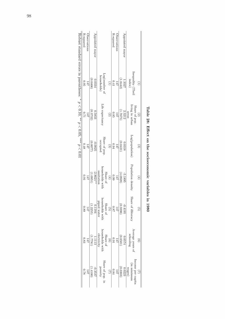
98
Table
28:
Eff
ect
on
the
socio
econom
icvaria
ble
sin
1980
(1)
(2)
(3)
(4)
(5)
(6)
(7)
Ineq
uality
(Theil
index
)
Share
of
pop
.liv
ing
inu
rban
area
sL
og(p
op
ula
tion
)P
op
ula
tion
den
sityS
hare
of
illiteracy
Avera
ge
yea
rsof
schoolin
g
Inco
me
per
capita
(inm
inim
um
wages)
Ap
poin
tedm
ayor
1.3
327
2.3
212
0.0
318
-5.1
895
-0.4
195
0.0
574
0.0
223
(1.8
442)
(1.7
675)
(0.0
421)
(4.0
928)
(0.9
396)
(0.0
501)
(0.0
303)
Observ
atio
ns
147
147
147
147
147
147
147
R-sq
uared
0.4
10.8
50.9
40.9
90.8
70.9
10.8
4(1
)(2
)(3
)(4
)(5
)(6
)(7
)
Log(n
um
ber
of
hou
sehold
s)L
ifeex
pecta
ncy
Share
of
pop
.occu
pied
Share
of
hou
sehold
sw
ithsa
nita
tion
Share
of
hou
sehold
sw
ithp
iped
water
Share
of
hou
sehold
sw
ithelectricity
Share
of
pop
.in
poverty
Ap
poin
tedm
ayor
0.0
334
0.5
833
-0.0
025
-2.8
621∗∗
0.1
184
1.1
113
-0.3
537
(0.0
406)
(0.3
732)
(0.0
077)
(1.0
951)
(1.2
255)
(1.7
781)
(1.4
100)
Observ
atio
ns
147
147
147
147
147
147
147
R-sq
uared
0.9
50.7
10.4
80.9
10.8
90.8
30.7
8
Rob
ust
stand
arderrors
inp
aren
theses:
∗p<
0.1
0,∗∗
p<
0.05,∗∗∗
p<
0.01

99
Table
29:
Eff
ect
on
the
socio
econom
icvari
able
sin
1991
(1)
(2)
(3)
(4)
(5)
(6)
(7)
Ineq
uality
(Thei
lin
dex
)
Share
of
pop
.livin
gin
urb
an
are
as
Log(p
op
ula
tion
)P
op
ula
tion
den
sity
Share
of
illite
racy
Aver
age
yea
rsof
schooling
Inco
me
per
capit
a(i
nm
inim
um
wages
)A
pp
oin
ted
mayor
4.3
194∗∗
2.5
252
0.1
214∗∗
-11.8
986
0.2
192
0.0
496
-0.0
043
(2.0
024)
(2.0
813)
(0.0
613)
(8.0
273)
(1.0
994)
(0.0
788)
(0.0
296)
Obse
rvati
on
s147
147
147
147
147
147
147
R-s
qu
are
d0.2
80.7
70.8
90.9
70.8
10.8
70.8
3(1
)(2
)(3
)(4
)(5
)(6
)(7
)
Log(n
um
ber
of
hou
sehold
s)L
ife
exp
ecta
ncy
Share
of
pop
.occ
up
ied
Share
of
hou
seh
old
sw
ith
sanit
ati
on
Share
of
hou
sehold
sw
ith
pip
edw
ate
r
Share
of
hou
sehold
sw
ith
elec
tric
ity
Share
of
pop
.in
pover
ty
Ap
poin
ted
mayor
0.1
135∗
0.0
579
-0.3
621
-0.0
199
-0.0
088
-0.0
058
1.1
380
(0.0
600)
(0.4
621)
(0.8
803)
(0.0
224)
(0.0
171)
(0.0
213)
(1.3
874)
Obse
rvati
on
s147
147
147
147
147
147
147
R-s
qu
are
d0.9
00.6
40.6
80.7
70.8
30.6
10.8
1
Rob
ust
stan
dar
der
rors
inp
aren
thes
es:
∗p<
0.1
0,∗∗
p<
0.05,∗∗
∗p<
0.01

100
Appendix B
Table 30: Possible selection in Globo’s coverage
Dependent variable=1 if Globo coverage in year tGlobo coverage=1 if municipality receives Globo signal 6 months before the election
(1) (2) (3) (4) (5) (6)ARENA vote-sharet-1 -0.0001
(0.0005)∆ ARENA vote-sharet-2,t-1 -0.0005
(0.0003)Turnoutt-1 0.0013
(0.0011)∆ Turnoutt-1,t-2 -0.0018∗∗
(0.0008)Share of blank votest-1 0.0006
(0.0009)∆ Blank + Null votest-2,t-1 0.0011∗
(0.0006)log(population) -0.2561∗∗∗ -0.0502∗∗∗ -0.2581∗∗∗ -0.0497∗∗∗ -0.2583∗∗∗ -0.0502∗∗∗
(0.0429) (0.0078) (0.0430) (0.0078) (0.0429) (0.0078)Share of pop living in urban areas -0.0010 -0.0008 -0.0010 -0.0007 -0.0010 -0.0008
(0.0013) (0.0005) (0.0013) (0.0005) (0.0013) (0.0005)Income per capita (in min wages) 0.1134∗∗ -0.0614∗∗ 0.1138∗∗ -0.0598∗∗ 0.1144∗∗ -0.0571∗
(0.0571) (0.0299) (0.0569) (0.0298) (0.0571) (0.0298)Average years of schooling 0.0478 0.1252∗∗∗ 0.0501 0.1236∗∗∗ 0.0497 0.1229∗∗∗
(0.0419) (0.0215) (0.0420) (0.0215) (0.0419) (0.0215)Life expectancy 0.0805∗∗∗ -0.0237∗∗∗ 0.0802∗∗∗ -0.0241∗∗∗ 0.0799∗∗∗ -0.0240∗∗∗
(0.0086) (0.0041) (0.0086) (0.0041) (0.0086) (0.0041)Infant mortality (per 1000) 0.0110∗∗∗ -0.0040∗∗∗ 0.0109∗∗∗ -0.0040∗∗∗ 0.0109∗∗∗ -0.0040∗∗∗
(0.0011) (0.0004) (0.0011) (0.0004) (0.0011) (0.0004)Share of illiterate over 15 y.o. -0.0011 0.0021∗ -0.0010 0.0022∗ -0.0011 0.0019
(0.0018) (0.0012) (0.0018) (0.0012) (0.0018) (0.0012)Share of employed people 0.0036 0.0037∗∗ 0.0035 0.0037∗∗ 0.0038 0.0036∗∗
(0.0024) (0.0015) (0.0024) (0.0015) (0.0024) (0.0015)Gini -0.5567∗∗∗ -0.2430∗∗ -0.5526∗∗∗ -0.2339∗ -0.5761∗∗∗ -0.2316∗
(0.1369) (0.1196) (0.1366) (0.1200) (0.1373) (0.1198)Wealth index -0.0978∗∗∗ 0.0273∗ -0.0982∗∗∗ 0.0293∗∗ -0.1001∗∗∗ 0.0264∗
(0.0277) (0.0142) (0.0277) (0.0141) (0.0277) (0.0141)Share of households with TV -0.0004 0.0047∗∗∗ -0.0003 0.0047∗∗∗ -0.0004 0.0047∗∗∗
(0.0011) (0.0007) (0.0011) (0.0007) (0.0011) (0.0007)year == 1982 0.3043∗∗∗ 0.2980∗∗∗ 0.3091∗∗∗
(0.0341) (0.0347) (0.0344)Municipality FE Yes No Yes No Yes NoObservations 7428 3699 7429 3700 7421 3692R-squared 0.79 0.27 0.79 0.27 0.79 0.27Mean 0.45 0.66 0.45 0.66 0.45 0.66
Note: Year and municipality fixed-effects were used in all specificationsStandard errors clustered at the municipality level in parentheses: ∗ p < 0.10, ∗∗ p < 0.05, ∗∗∗ p < 0.01
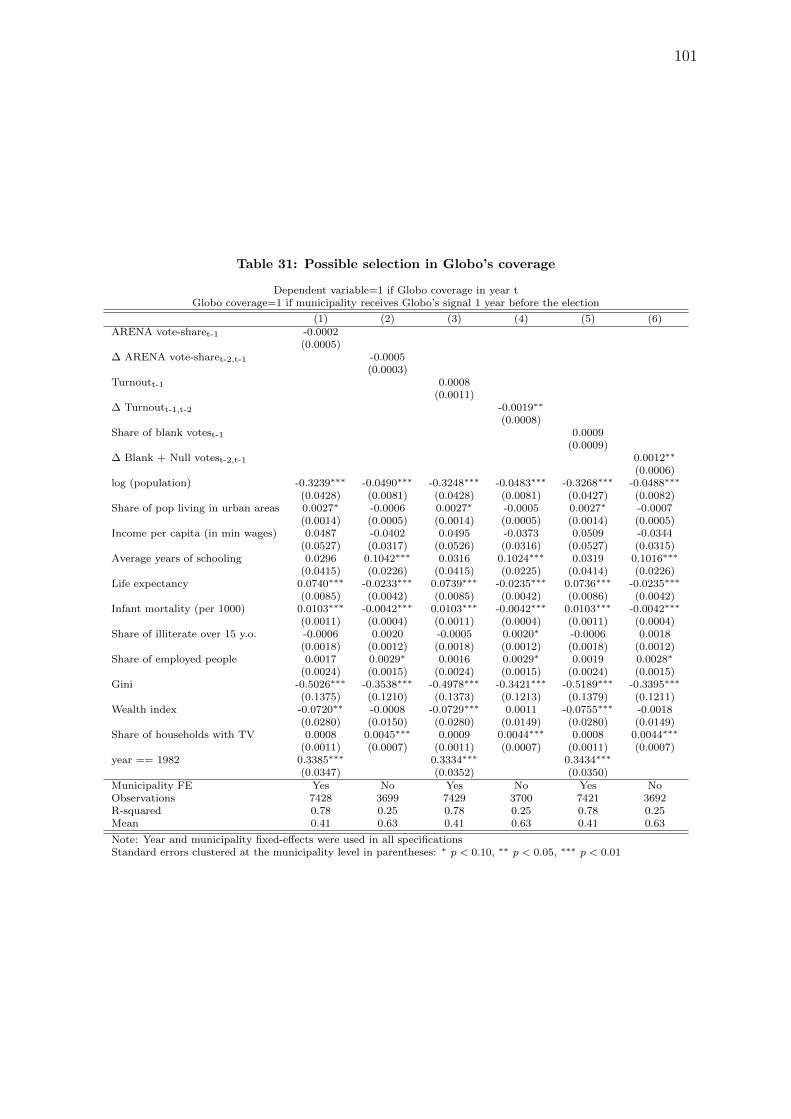
101
Table 31: Possible selection in Globo’s coverage
Dependent variable=1 if Globo coverage in year tGlobo coverage=1 if municipality receives Globo’s signal 1 year before the election
(1) (2) (3) (4) (5) (6)ARENA vote-sharet-1 -0.0002
(0.0005)∆ ARENA vote-sharet-2,t-1 -0.0005
(0.0003)Turnoutt-1 0.0008
(0.0011)∆ Turnoutt-1,t-2 -0.0019∗∗
(0.0008)Share of blank votest-1 0.0009
(0.0009)∆ Blank + Null votest-2,t-1 0.0012∗∗
(0.0006)log (population) -0.3239∗∗∗ -0.0490∗∗∗ -0.3248∗∗∗ -0.0483∗∗∗ -0.3268∗∗∗ -0.0488∗∗∗
(0.0428) (0.0081) (0.0428) (0.0081) (0.0427) (0.0082)Share of pop living in urban areas 0.0027∗ -0.0006 0.0027∗ -0.0005 0.0027∗ -0.0007
(0.0014) (0.0005) (0.0014) (0.0005) (0.0014) (0.0005)Income per capita (in min wages) 0.0487 -0.0402 0.0495 -0.0373 0.0509 -0.0344
(0.0527) (0.0317) (0.0526) (0.0316) (0.0527) (0.0315)Average years of schooling 0.0296 0.1042∗∗∗ 0.0316 0.1024∗∗∗ 0.0319 0.1016∗∗∗
(0.0415) (0.0226) (0.0415) (0.0225) (0.0414) (0.0226)Life expectancy 0.0740∗∗∗ -0.0233∗∗∗ 0.0739∗∗∗ -0.0235∗∗∗ 0.0736∗∗∗ -0.0235∗∗∗
(0.0085) (0.0042) (0.0085) (0.0042) (0.0086) (0.0042)Infant mortality (per 1000) 0.0103∗∗∗ -0.0042∗∗∗ 0.0103∗∗∗ -0.0042∗∗∗ 0.0103∗∗∗ -0.0042∗∗∗
(0.0011) (0.0004) (0.0011) (0.0004) (0.0011) (0.0004)Share of illiterate over 15 y.o. -0.0006 0.0020 -0.0005 0.0020∗ -0.0006 0.0018
(0.0018) (0.0012) (0.0018) (0.0012) (0.0018) (0.0012)Share of employed people 0.0017 0.0029∗ 0.0016 0.0029∗ 0.0019 0.0028∗
(0.0024) (0.0015) (0.0024) (0.0015) (0.0024) (0.0015)Gini -0.5026∗∗∗ -0.3538∗∗∗ -0.4978∗∗∗ -0.3421∗∗∗ -0.5189∗∗∗ -0.3395∗∗∗
(0.1375) (0.1210) (0.1373) (0.1213) (0.1379) (0.1211)Wealth index -0.0720∗∗ -0.0008 -0.0729∗∗∗ 0.0011 -0.0755∗∗∗ -0.0018
(0.0280) (0.0150) (0.0280) (0.0149) (0.0280) (0.0149)Share of households with TV 0.0008 0.0045∗∗∗ 0.0009 0.0044∗∗∗ 0.0008 0.0044∗∗∗
(0.0011) (0.0007) (0.0011) (0.0007) (0.0011) (0.0007)year == 1982 0.3385∗∗∗ 0.3334∗∗∗ 0.3434∗∗∗
(0.0347) (0.0352) (0.0350)Municipality FE Yes No Yes No Yes NoObservations 7428 3699 7429 3700 7421 3692R-squared 0.78 0.25 0.78 0.25 0.78 0.25Mean 0.41 0.63 0.41 0.63 0.41 0.63
Note: Year and municipality fixed-effects were used in all specificationsStandard errors clustered at the municipality level in parentheses: ∗ p < 0.10, ∗∗ p < 0.05, ∗∗∗ p < 0.01

102
Table 32: Effect of Globo on ARENA’s vote-share
Dependent variable: ARENA’s vote-share in t, t=1972, 1976, 1982Globo coverage=1 if municipality receives Globo’s signal 6 months before the election
(1) (2) (3)ARENA Turnout Blank and null
Globo * year==1972 4.1694∗∗∗ -0.9291 -0.2570(1.5819) (0.5777) (0.8033)
Globo * year==1976 -2.2179∗∗ -0.7642∗∗ -0.1681(0.8677) (0.3311) (0.3886)
Globo * year==1982 -2.4453∗∗ 1.3079∗∗∗ -0.1263(1.0528) (0.4451) (0.4069)
log(population) -5.9612∗∗∗ -2.7450∗∗∗ 2.2221∗∗∗
(1.5471) (0.6606) (0.5541)Share of pop living in urban areas -0.1913∗∗∗ -0.0287 0.0210
(0.0510) (0.0188) (0.0175)Income per capita (in min wages) -2.7047 1.8041∗∗∗ -2.0125∗∗∗
(2.1095) (0.5825) (0.5941)Average years of schooling -6.1607∗∗∗ -0.7126 0.8536
(1.5726) (0.6390) (0.6214)Life expectancy -0.6553∗ 0.2782∗∗ -0.2899∗∗
(0.3377) (0.1352) (0.1345)Infant mortality (per 1000) -0.0467 0.0358∗ -0.0437∗∗
(0.0468) (0.0189) (0.0182)Share of illiterate over 15 y.o. -0.0146 -0.0571∗ 0.0532∗
(0.0721) (0.0318) (0.0296)Share of employed people 0.0531 0.0269 -0.0333
(0.0919) (0.0376) (0.0332)Gini 3.9989 -7.7178∗∗∗ -0.4949
(5.5809) (2.2965) (2.1943)Wealth index -0.6947 -0.1348 1.0327∗∗∗
(1.0302) (0.3970) (0.3765)Share of households with TV -0.0844∗∗ -0.0600∗∗∗ 0.0093
(0.0416) (0.0153) (0.0149)year == 1976 -4.2668∗∗∗ 4.0947∗∗∗ -4.2041∗∗∗
(0.4840) (0.2198) (0.2844)year == 1982 -3.9935∗∗∗ 4.4651∗∗∗ -1.4678∗∗
(1.4955) (0.5946) (0.5816)Observations 11206 11209 11200R-squared 0.69 0.72 0.43Mean 67.48 79.91 8.45
Note: Year and municipality fixed-effects were used in all specificationsStandard errors clustered at the municipality level in parentheses: ∗ p < 0.10, ∗∗ p < 0.05, ∗∗∗ p < 0.01

103
Table 33: Effect of Globo on ARENA’s vote-share
Dependent variable: ARENA’s vote-share in t, t=1972, 1976, 1982Globo coverage=1 if municipality receives Globo’s signal 1 year before the election
(1) (2) (3)ARENA Turnout Blank and null
Globo * year==1972 4.0247∗∗ -1.4135∗∗ 0.0905(1.8611) (0.5912) (0.8825)
Globo * year==1976 -3.6608∗∗∗ -0.9497∗∗∗ 0.2298(0.9285) (0.3612) (0.4399)
Globo * year==1982 -2.6027∗∗ 1.0612∗∗ 0.4262(1.0192) (0.4234) (0.3896)
log (population) -6.1348∗∗∗ -2.9030∗∗∗ 2.3680∗∗∗
(1.5456) (0.6657) (0.5582)Share of pop living in urban areas -0.1854∗∗∗ -0.0275 0.0203
(0.0509) (0.0189) (0.0174)Income per capita (in min wages) -2.8223 1.7758∗∗∗ -2.0541∗∗∗
(2.1083) (0.5843) (0.5906)Average years of schooling -6.1887∗∗∗ -0.6983 0.8513
(1.5721) (0.6385) (0.6212)Life expectancy -0.6106∗ 0.2814∗∗ -0.3307∗∗
(0.3368) (0.1351) (0.1338)Infant mortality (per 1000) -0.0392 0.0360∗ -0.0493∗∗∗
(0.0467) (0.0189) (0.0181)Share of illiterate over 15 y.o. -0.0133 -0.0576∗ 0.0532∗
(0.0721) (0.0318) (0.0296)Share of employed people 0.0507 0.0276 -0.0349
(0.0916) (0.0376) (0.0332)Gini 4.3031 -7.8912∗∗∗ -0.2375
(5.5768) (2.2932) (2.1968)Wealth index -0.7353 -0.1130 1.0643∗∗∗
(1.0279) (0.3979) (0.3755)Share of households with TV -0.0871∗∗ -0.0582∗∗∗ 0.0071
(0.0415) (0.0152) (0.0149)year == 1976 -4.2500∗∗∗ 4.0754∗∗∗ -4.2595∗∗∗
(0.4680) (0.2110) (0.2726)year == 1982 -3.9522∗∗∗ 4.6020∗∗∗ -1.6996∗∗∗
(1.4741) (0.5877) (0.5803)Observations 11206 11209 11200R-squared 0.69 0.72 0.43Mean 67.48 79.91 8.45
Note: Year and municipality fixed-effects were used in all specificationsStandard errors clustered at the municipality level in parentheses: ∗ p < 0.10, ∗∗ p < 0.05, ∗∗∗ p < 0.01

104
Table 34: Possible selection in Globo’s coverage (Turnout)
Dependent variable=1 if Globo coverage in year t, t=1976, 1982
(1) (2) (3) (4) (5)Turnoutt-1 0.0096∗∗∗ 0.0029∗∗∗ 0.0013
(0.0005) (0.0006) (0.0011)∆ Turnoutt-1,t-2 -0.0035∗∗∗ -0.0019∗∗
(0.0009) (0.0008)log(population) -0.0404∗∗∗ -0.2748∗∗∗ -0.0486∗∗∗
(0.0065) (0.0429) (0.0078)Share of pop living in urban areas 0.0002 -0.0007 -0.0007
(0.0004) (0.0013) (0.0005)Income per capita (in min wages) -0.0109 0.0705 -0.0658∗∗
(0.0249) (0.0554) (0.0298)Average years of schooling 0.0610∗∗∗ 0.0718∗ 0.1245∗∗∗
(0.0172) (0.0418) (0.0214)Life expectancy 0.0025 0.0815∗∗∗ -0.0236∗∗∗
(0.0028) (0.0086) (0.0041)Infant mortality (per 1.000 habitants) -0.0005∗ 0.0110∗∗∗ -0.0040∗∗∗
(0.0003) (0.0011) (0.0004)Share of illiterate over 15 y.o. -0.0003 -0.0009 0.0021∗
(0.0008) (0.0018) (0.0012)Share of employed people 0.0021∗ 0.0039 0.0038∗∗
(0.0012) (0.0024) (0.0015)Gini -0.4030∗∗∗ -0.5512∗∗∗ -0.2477∗∗
(0.0749) (0.1372) (0.1198)Wealth index -0.0081 -0.0921∗∗∗ 0.0316∗∗
(0.0105) (0.0278) (0.0140)Share of households with TV 0.0051∗∗∗ -0.0009 0.0047∗∗∗
(0.0006) (0.0011) (0.0007)year == 1982 0.3707∗∗∗ 0.2021∗∗∗ 0.3061∗∗∗
(0.0089) (0.0146) (0.0347)Municipality FE No No Yes No NoObservations 7429 7429 7429 3700 3700R-squared 0.21 0.31 0.79 0.00 0.27Mean 0.46 0.46 0.46 0.66 0.66
Standard errors clustered at the municipality level in parentheses: ∗ p < 0.10, ∗∗ p < 0.05, ∗∗∗ p < 0.01
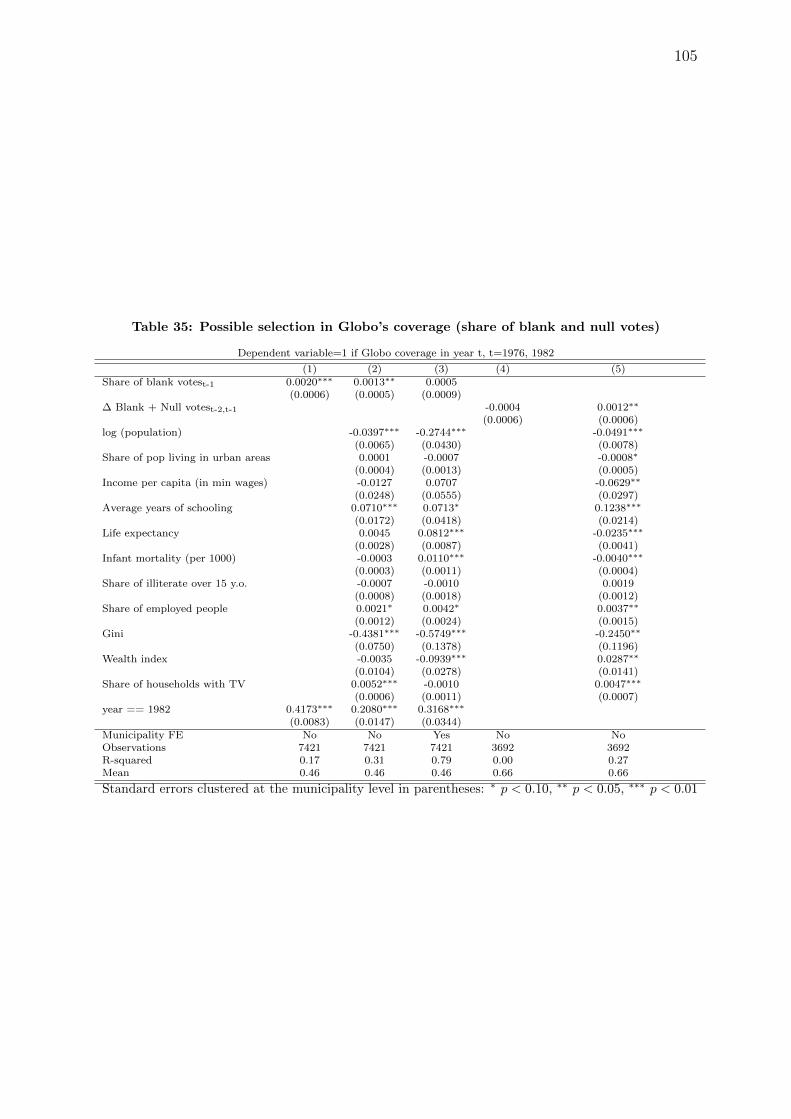
105
Table 35: Possible selection in Globo’s coverage (share of blank and null votes)
Dependent variable=1 if Globo coverage in year t, t=1976, 1982
(1) (2) (3) (4) (5)Share of blank votest-1 0.0020∗∗∗ 0.0013∗∗ 0.0005
(0.0006) (0.0005) (0.0009)∆ Blank + Null votest-2,t-1 -0.0004 0.0012∗∗
(0.0006) (0.0006)log (population) -0.0397∗∗∗ -0.2744∗∗∗ -0.0491∗∗∗
(0.0065) (0.0430) (0.0078)Share of pop living in urban areas 0.0001 -0.0007 -0.0008∗
(0.0004) (0.0013) (0.0005)Income per capita (in min wages) -0.0127 0.0707 -0.0629∗∗
(0.0248) (0.0555) (0.0297)Average years of schooling 0.0710∗∗∗ 0.0713∗ 0.1238∗∗∗
(0.0172) (0.0418) (0.0214)Life expectancy 0.0045 0.0812∗∗∗ -0.0235∗∗∗
(0.0028) (0.0087) (0.0041)Infant mortality (per 1000) -0.0003 0.0110∗∗∗ -0.0040∗∗∗
(0.0003) (0.0011) (0.0004)Share of illiterate over 15 y.o. -0.0007 -0.0010 0.0019
(0.0008) (0.0018) (0.0012)Share of employed people 0.0021∗ 0.0042∗ 0.0037∗∗
(0.0012) (0.0024) (0.0015)Gini -0.4381∗∗∗ -0.5749∗∗∗ -0.2450∗∗
(0.0750) (0.1378) (0.1196)Wealth index -0.0035 -0.0939∗∗∗ 0.0287∗∗
(0.0104) (0.0278) (0.0141)Share of households with TV 0.0052∗∗∗ -0.0010 0.0047∗∗∗
(0.0006) (0.0011) (0.0007)year == 1982 0.4173∗∗∗ 0.2080∗∗∗ 0.3168∗∗∗
(0.0083) (0.0147) (0.0344)Municipality FE No No Yes No NoObservations 7421 7421 7421 3692 3692R-squared 0.17 0.31 0.79 0.00 0.27Mean 0.46 0.46 0.46 0.66 0.66
Standard errors clustered at the municipality level in parentheses: ∗ p < 0.10, ∗∗ p < 0.05, ∗∗∗ p < 0.01

106
Table 36: Effect of Globo on turnout vote-shareDependent variable: Turnout in t, t=1972, 1976, 1982
(1) (2) (3) (4) (5) (6)Globo 5.2077∗∗∗ 1.3639∗∗∗ 0.1308
(0.2478) (0.2337) (0.3110)Globo * year==1972 4.5688∗∗∗ 2.0127∗∗∗ -0.9373
(0.5907) (0.5369) (0.5757)Globo * year==1976 4.0400∗∗∗ 1.7103∗∗∗ -0.7704∗∗
(0.3285) (0.2930) (0.3254)Globo * year==1982 6.3774∗∗∗ 0.7728∗∗ 1.2665∗∗∗
(0.3063) (0.3223) (0.4466)log (population) -0.7449∗∗∗ -2.8995∗∗∗ -0.7631∗∗∗ -2.7589∗∗∗
(0.1285) (0.6664) (0.1286) (0.6614)Share of pop living in urban areas -0.0082 -0.0276 -0.0102 -0.0285
(0.0075) (0.0191) (0.0075) (0.0189)Income per capita (in min wages) -1.1826∗∗ 1.9884∗∗∗ -1.1306∗∗ 1.7987∗∗∗
(0.5314) (0.5792) (0.5299) (0.5832)Average years of schooling 4.4156∗∗∗ -0.7347 4.4382∗∗∗ -0.7005
(0.3708) (0.6424) (0.3704) (0.6394)Life expectancy 0.4664∗∗∗ 0.3350∗∗ 0.4629∗∗∗ 0.2791∗∗
(0.0538) (0.1345) (0.0537) (0.1352)Infant mortality (per 1000) 0.0561∗∗∗ 0.0432∗∗ 0.0556∗∗∗ 0.0359∗
(0.0051) (0.0188) (0.0051) (0.0189)Share of illiterate over 15 y.o. -0.0754∗∗∗ -0.0569∗ -0.0735∗∗∗ -0.0569∗
(0.0166) (0.0318) (0.0167) (0.0318)Share of employed people 0.0145 0.0295 0.0144 0.0273
(0.0238) (0.0375) (0.0238) (0.0376)Gini -7.5858∗∗∗ -8.4621∗∗∗ -7.5126∗∗∗ -7.7513∗∗∗
(1.6818) (2.2927) (1.6813) (2.2978)Wealth index 1.7612∗∗∗ -0.0521 1.7686∗∗∗ -0.1358
(0.1999) (0.3978) (0.1992) (0.3971)Share of households with TV 0.0484∗∗∗ -0.0466∗∗∗ 0.0524∗∗∗ -0.0601∗∗∗
(0.0110) (0.0148) (0.0112) (0.0153)year == 1976 3.1042∗∗∗ 3.7430∗∗∗ 3.9650∗∗∗ 3.3438∗∗∗ 3.7099∗∗∗ 4.1023∗∗∗
(0.1689) (0.1657) (0.2012) (0.1912) (0.1877) (0.2218)year == 1982 1.2979∗∗∗ -0.7264∗∗ 4.9059∗∗∗ 0.4746∗ -0.3851 4.4822∗∗∗
(0.2299) (0.3185) (0.5816) (0.2880) (0.3415) (0.5956)Municipality FE No No Yes No No YesObservations 11209 11209 11209 11209 11209 11209R-squared 0.08 0.27 0.72 0.08 0.27 0.72Mean 79.91 79.91 79.91 79.91 79.91 79.91
Standard errors clustered at the municipality level in parentheses: ∗ p < 0.10, ∗∗ p < 0.05, ∗∗∗ p < 0.01
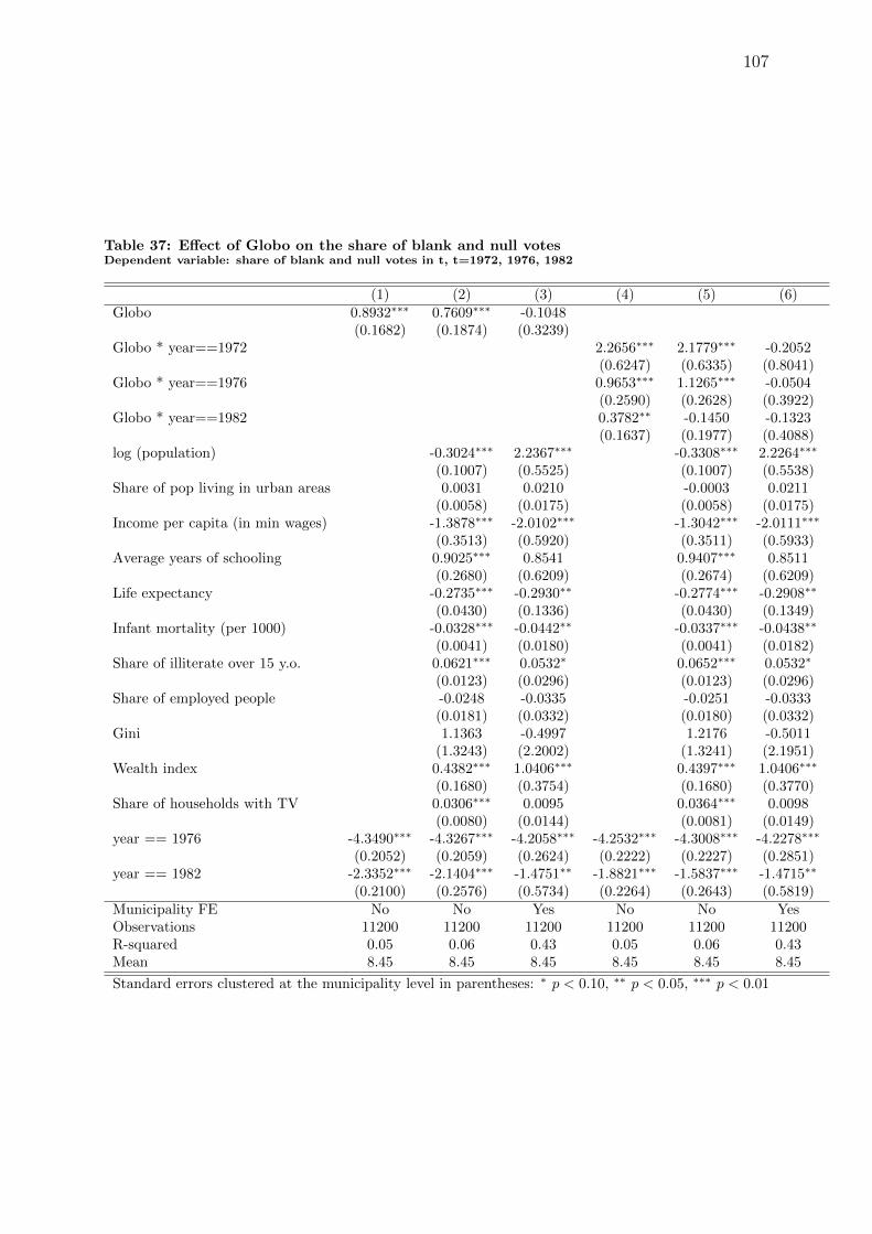
107
Table 37: Effect of Globo on the share of blank and null votesDependent variable: share of blank and null votes in t, t=1972, 1976, 1982
(1) (2) (3) (4) (5) (6)Globo 0.8932∗∗∗ 0.7609∗∗∗ -0.1048
(0.1682) (0.1874) (0.3239)Globo * year==1972 2.2656∗∗∗ 2.1779∗∗∗ -0.2052
(0.6247) (0.6335) (0.8041)Globo * year==1976 0.9653∗∗∗ 1.1265∗∗∗ -0.0504
(0.2590) (0.2628) (0.3922)Globo * year==1982 0.3782∗∗ -0.1450 -0.1323
(0.1637) (0.1977) (0.4088)log (population) -0.3024∗∗∗ 2.2367∗∗∗ -0.3308∗∗∗ 2.2264∗∗∗
(0.1007) (0.5525) (0.1007) (0.5538)Share of pop living in urban areas 0.0031 0.0210 -0.0003 0.0211
(0.0058) (0.0175) (0.0058) (0.0175)Income per capita (in min wages) -1.3878∗∗∗ -2.0102∗∗∗ -1.3042∗∗∗ -2.0111∗∗∗
(0.3513) (0.5920) (0.3511) (0.5933)Average years of schooling 0.9025∗∗∗ 0.8541 0.9407∗∗∗ 0.8511
(0.2680) (0.6209) (0.2674) (0.6209)Life expectancy -0.2735∗∗∗ -0.2930∗∗ -0.2774∗∗∗ -0.2908∗∗
(0.0430) (0.1336) (0.0430) (0.1349)Infant mortality (per 1000) -0.0328∗∗∗ -0.0442∗∗ -0.0337∗∗∗ -0.0438∗∗
(0.0041) (0.0180) (0.0041) (0.0182)Share of illiterate over 15 y.o. 0.0621∗∗∗ 0.0532∗ 0.0652∗∗∗ 0.0532∗
(0.0123) (0.0296) (0.0123) (0.0296)Share of employed people -0.0248 -0.0335 -0.0251 -0.0333
(0.0181) (0.0332) (0.0180) (0.0332)Gini 1.1363 -0.4997 1.2176 -0.5011
(1.3243) (2.2002) (1.3241) (2.1951)Wealth index 0.4382∗∗∗ 1.0406∗∗∗ 0.4397∗∗∗ 1.0406∗∗∗
(0.1680) (0.3754) (0.1680) (0.3770)Share of households with TV 0.0306∗∗∗ 0.0095 0.0364∗∗∗ 0.0098
(0.0080) (0.0144) (0.0081) (0.0149)year == 1976 -4.3490∗∗∗ -4.3267∗∗∗ -4.2058∗∗∗ -4.2532∗∗∗ -4.3008∗∗∗ -4.2278∗∗∗
(0.2052) (0.2059) (0.2624) (0.2222) (0.2227) (0.2851)year == 1982 -2.3352∗∗∗ -2.1404∗∗∗ -1.4751∗∗ -1.8821∗∗∗ -1.5837∗∗∗ -1.4715∗∗
(0.2100) (0.2576) (0.5734) (0.2264) (0.2643) (0.5819)Municipality FE No No Yes No No YesObservations 11200 11200 11200 11200 11200 11200R-squared 0.05 0.06 0.43 0.05 0.06 0.43Mean 8.45 8.45 8.45 8.45 8.45 8.45
Standard errors clustered at the municipality level in parentheses: ∗ p < 0.10, ∗∗ p < 0.05, ∗∗∗ p < 0.01

108
Table
38:
Hete
rogeneous
eff
ects
by
novela
conte
nt
Dep
end
ent
varia
ble:
AR
EN
A’s
vote-sh
are
inm
unicip
al
election
sin
t,t=
1972,
1976,
1982
Conten
tm
easu
re:N
um
ber
of
novela
sw
ithsp
ecific
plo
tb
etween
election
sin
t-1an
dt.
PanelA:Politic
al-r
elate
dplots
(part1
)
Politica
lissu
esP
olitica
lissu
es(m
ain
plo
t)P
olitica
lissu
es(seco
ndary
plo
t)P
olitica
lch
ara
cter(m
ain
)P
olitica
lch
ara
cter(seco
ndary
)(1
)(2
)(3
)(4
)(5
)G
lob
o-0
.6337
-0.7
756
-0.6
140
-0.6
682
-1.9
645∗∗
(0.8
940)
(0.8
637)
(0.9
731)
(0.8
805)
(0.9
179)
Plo
t-1
1.0
823∗∗
-12.6
215∗∗
-45.0
496∗
-18.8
980∗∗
16.0
579
(5.1
037)
(5.9
342)
(27.2
658)
(8.6
066)
(24.4
114)
Observ
atio
ns
11206
11206
11206
11206
11206
R-sq
uared
0.6
90.6
90.6
90.6
90.6
9M
ean
67.4
867.4
867.4
867.4
867.4
8
PanelB:Politic
al-r
elate
dplots
(part2
)C
orru
ptio
nE
lections
Pub
licreso
urces
Dem
ocra
cyO
ther
politica
lissu
es(1
)(2
)(3
)(4
)(5
)G
lob
o-0
.8498
-0.5
195
-0.9
613
-0.4
270
-0.7
042
(0.8
677)
(0.8
998)
(0.7
963)
(0.8
752)
(0.8
713)
Plo
t-1
8.0
981∗∗
-24.0
053∗∗∗
-32.9
955∗∗∗
-26.4
689∗∗∗
-13.0
459∗∗
(8.4
402)
(9.2
903)
(10.7
854)
(8.5
708)
(5.8
453)
Observ
atio
ns
11206
11206
11206
11206
11206
R-sq
uared
0.6
90.6
90.6
90.6
90.6
9M
ean
67.4
867.4
867.4
867.4
867.4
8
PanelC:Non-p
olitic
alplots
Histo
rical
Ru
ral
Perip
hery
Preju
dice
Sla
very
(1)
(2)
(3)
(4)
(5)
glo
bo
-1.4
245
-0.6
472
-1.0
505
-1.3
276
-0.7
801
(0.8
879)
(0.9
036)
(0.8
498)
(0.8
361)
(0.8
433)
plo
t-1
.9986
-4.6
289∗∗
-5.6
485
-1.6
715
-23.9
872∗∗
(5.4
295)
(2.1
172)
(3.4
505)
(2.4
709)
(9.3
553)
Observ
atio
ns
11206
11206
11206
11206
11206
R-sq
uared
0.6
90.6
90.6
90.6
90.6
9M
ean
67.4
867.4
867.4
867.4
867.4
8
Sta
nd
ard
errors
clustered
at
the
mu
nicip
ality
level
inparen
theses:
∗p<
0.1
0,∗∗
p<
0.0
5,∗∗∗
p<
0.0
1
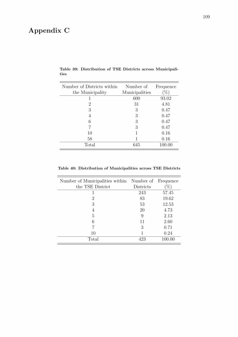
109
Appendix C
Table 39: Distribution of TSE Districts across Municipali-ties
Number of Districts within Number of Frequencethe Municipality Municipalities (%)
1 600 93.022 31 4.813 3 0.474 3 0.476 3 0.477 3 0.4710 1 0.1658 1 0.16
Total 645 100.00
Table 40: Distribution of Municipalities across TSE Districts
Number of Municipalities within Number of Frequencethe TSE District Districts (%)
1 243 57.452 83 19.623 53 12.534 20 4.735 9 2.136 11 2.607 3 0.7110 1 0.24
Total 423 100.00
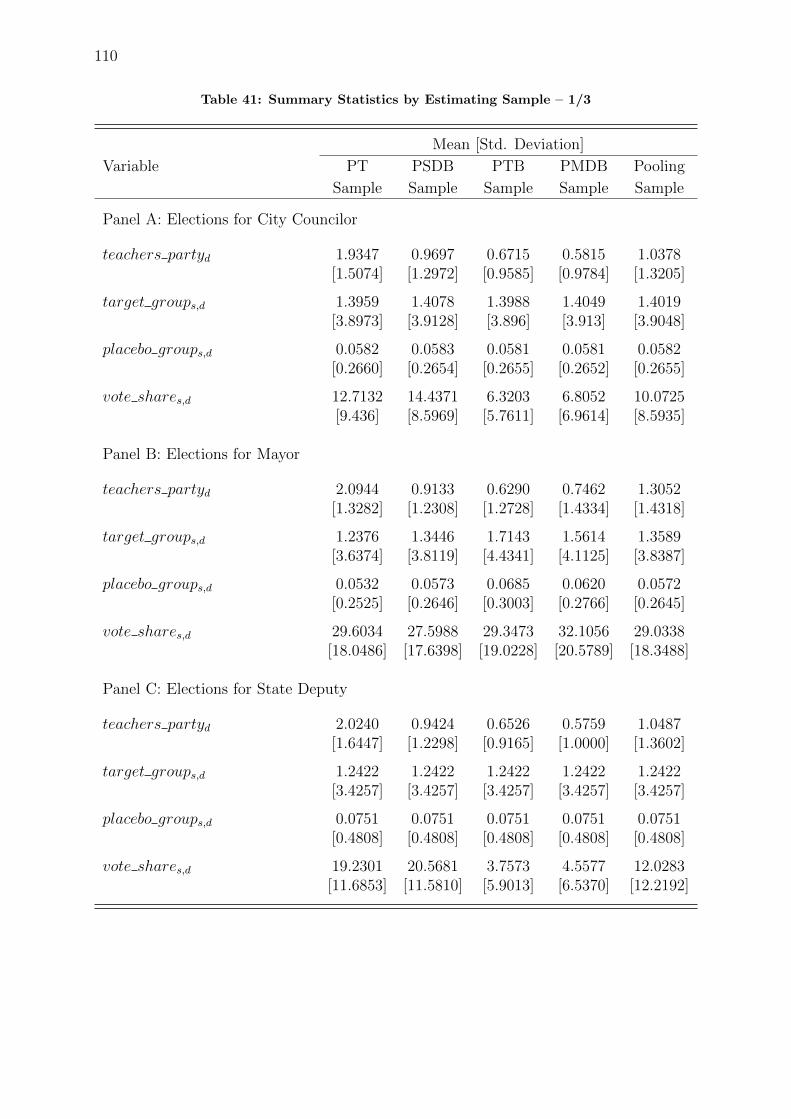
110
Table 41: Summary Statistics by Estimating Sample – 1/3
Variable
Mean [Std. Deviation]
PT PSDB PTB PMDB Pooling
Sample Sample Sample Sample Sample
Panel A: Elections for City Councilor
teachers partyd 1.9347 0.9697 0.6715 0.5815 1.0378[1.5074] [1.2972] [0.9585] [0.9784] [1.3205]
target groups,d 1.3959 1.4078 1.3988 1.4049 1.4019[3.8973] [3.9128] [3.896] [3.913] [3.9048]
placebo groups,d 0.0582 0.0583 0.0581 0.0581 0.0582[0.2660] [0.2654] [0.2655] [0.2652] [0.2655]
vote shares,d 12.7132 14.4371 6.3203 6.8052 10.0725[9.436] [8.5969] [5.7611] [6.9614] [8.5935]
Panel B: Elections for Mayor
teachers partyd 2.0944 0.9133 0.6290 0.7462 1.3052[1.3282] [1.2308] [1.2728] [1.4334] [1.4318]
target groups,d 1.2376 1.3446 1.7143 1.5614 1.3589[3.6374] [3.8119] [4.4341] [4.1125] [3.8387]
placebo groups,d 0.0532 0.0573 0.0685 0.0620 0.0572[0.2525] [0.2646] [0.3003] [0.2766] [0.2645]
vote shares,d 29.6034 27.5988 29.3473 32.1056 29.0338[18.0486] [17.6398] [19.0228] [20.5789] [18.3488]
Panel C: Elections for State Deputy
teachers partyd 2.0240 0.9424 0.6526 0.5759 1.0487[1.6447] [1.2298] [0.9165] [1.0000] [1.3602]
target groups,d 1.2422 1.2422 1.2422 1.2422 1.2422[3.4257] [3.4257] [3.4257] [3.4257] [3.4257]
placebo groups,d 0.0751 0.0751 0.0751 0.0751 0.0751[0.4808] [0.4808] [0.4808] [0.4808] [0.4808]
vote shares,d 19.2301 20.5681 3.7573 4.5577 12.0283[11.6853] [11.5810] [5.9013] [6.5370] [12.2192]

111
Table 42: Summary Statistics by Estimating Sample – 2/3
Variable
Mean [Std. Deviation]
PT PSDB PTB PMDB Pooling
Sample Sample Sample Sample Sample
Panel D: Elections for Federal Deputy
teachers partyd 2.0240 0.9424 0.6526 0.5759 1.0487[1.6447] [1.2298] [0.9165] [1.0000] [1.3602]
target groups,d 1.2422 1.2422 1.2422 1.2422 1.2422[3.4257] [3.4257] [3.4257] [3.4257] [3.4257]
placebo groups,d 0.0751 0.0751 0.0751 0.0751 0.0751[0.4808] [0.4808] [0.4808] [0.4808] [0.4808]
vote shares,d 16.3167 16.2179 2.7722 2.0545 9.3403[9.7816] [10.1069] [3.7867] [4.6703] [10.3220]
Panel E: Elections for Governor
teachers partyd 2.0240 0.9424 – – 1.4832[1.6447] [1.2298] [1.5496]
target groups,d 1.2422 1.2422 – – 1.2422[3.4257] [3.4257] [3.4257]
placebo groups,d 0.0751 0.0751 – – 0.0751[0.4808] [0.4808] [0.4808]
vote shares,d 31.5339 45.939 – – 38.7365[11.1309] [12.2659] [13.7496]
Panel F: Elections for President
teachers partyd 2.0240 0.9424 – – 1.4832[1.6447] [1.2298] [1.5496]
target groups,d 1.2422 1.2422 – – 1.2422[3.4257] [3.4257] [3.4257]
placebo groups,d 0.0751 0.0751 – – 0.0751[0.4808] [0.4808] [0.4808]
vote shares,d 34.5432 37.9579 – – 36.2506[12.3332] [12.5190] [12.5431]

112
Table 43: Summary Statistics by Estimating Sample – 3/3
Variable
Mean [Std. Deviation]
PT PSDB PTB PMDB Pooling
Sample Sample Sample Sample Sample
Panel G: Elections for Senator
teachers partyd 2.0240 0.9424 0.6526 – 1.2063[1.6447] [1.2298] [0.9165] [1.4262]
target groups,d 1.2422 1.2422 1.2422 – 1.2422[3.4257] [3.4257] [3.4257] [3.4257]
placebo groups,d 0.0751 0.0751 0.0751 – 0.0751[0.4808] [0.4808] [0.4808] [0.4808]
vote shares,d 16.4460 22.2648 7.9145 – 15.5418[6.5094] [6.3309] [2.7782] [8.0491]
Panel H: 2008 Local Elections
teachers partyd 1.9211 0.9691 0.6683 0.5785 1.0342[1.5334] [1.2978] [0.9609] [0.9768] [1.3271]
target groups,d 1.4097 1.4097 1.4097 1.4097 1.4097[3.9190] [3.9190] [3.9190] [3.9190] [3.9190]
turnouts,d 85.2729 85.2729 85.2729 85.2729 85.2729[4.5062] [4.5062] [4.5062] [4.5062] [4.5062]
Panel I: 2010 General Elections
teachers partyd 2.0240 0.9424 0.6526 0.5759 1.0487[1.6447] [1.2298] [0.9165] [1.0000] [1.3602]
target groups,d 1.2422 1.2422 1.2422 1.2422 1.2422[3.4257] [3.4257] [3.4257] [3.4257] [3.4257]
turnouts,d 83.6163 83.6163 83.6163 83.6163 83.6163[5.2672] [5.2672] [5.2672] [5.2672] [5.2672]

113
Figure 12: Municipalities in the State of Sao Paulo. Highlighted: City of Sao Paulo
Figure 13: Polling Districts in the City of Sao Paulo

114
Figure 14: A Public School Employed as a Polling Place
Source: http://www.cruzeirodovale.com.br/?eleicoes-2014-confira-os-eleitos-no-estado-de-santa-catarina&ctd=23932.
Figure 15: A Public School Classroom Used as a Polling Station
Source: http://www.cruzeirodovale.com.br/?eleicoes-2014-confira-os-eleitos-no-estado-de-santa-catarina&ctd=23932.