Embed Size (px)
Citation preview

Alex Avelino Carrasco Martinez
Demographics and Real Interest Rate in theUS economy
Dissertação de Mestrado
Thesis presented to the Programa de Pós–graduação em Econo-mia da PUC-Rio in partial fulfillment of the requirements for thedegree of Mestre em Economia.
Advisor: Prof. Carlos Viana de Carvalho
Rio de JaneiroNovember 2019

Alex Avelino Carrasco Martinez
Demographics and Real Interest Rate in theUS economy
Thesis presented to the Programa de Pós–graduação em Econo-mia da PUC-Rio in partial fulfillment of the requirements for the degree of Mestre em Economia. Approved by the Examination Committee.
Prof. Carlos Viana de CarvalhoAdvisor
Departamento de Economia – PUC-Rio
Prof. Andrea FerreroDepartment of Economics – Oxford University
Prof. Eduardo ZilbermanDepartamento de Economia – PUC-Rio
Rio de Janeiro, November the 11th, 2019

All rights reserved.
Alex Avelino Carrasco Martinez
B.A. in Economics by Federico Villareal National University(Lima, Peru), 2014.
Bibliographic dataCarrasco Martinez, Alex Avelino
Demographics and Real Interest Rate in the US economy/ Alex Avelino Carrasco Martinez; advisor: Carlos Viana deCarvalho. – Rio de janeiro: PUC-Rio, Departamento de Eco-nomia, 2019.
v., 53 f: il. color. ; 30 cm
Dissertação (mestrado) - Pontifícia Universidade Católicado Rio de Janeiro, Departamento de Economia.
Inclui bibliografia
1. Economia – Teses. 2. Macroeconomia – Teses. 3. Taxade fertilidade;. 4. Expectativa de vida;. 5. Transição Demo-gráfica;. 6. Taxa de juros real;. 7. Gerações sobrepostas.. I.Carvalho, Carlos Viana de. II. Pontifícia Universidade Católicado Rio de Janeiro. Departamento de Economia. III. Título.
CDD: 620.11

Acknowledgments
I thank my parents, Gregorio and Yldefonsa, and my siblings for their un-conditional love and support throughout my entire life. Specially, my motherhas almost all credits of my achievements. I would not have made it this farwithout you, I love you so much. I am also thankful to Ysabel, who enormouslyhas changed my life, for her tremendous support and comprehension duringthe last stage of this project.
I am grateful to my advisor, Prof. Carlos Viana de Carvalho, for his extraor-dinary guidance, encouragement, and patience. This dissertation would neverhave been possible without him. I thank Prof. Eduardo Zilberman and Prof.Andrea Ferrero for accepting the invite to be in the Examination Committee.
I also thank my professors of the Department of Economics at PUC-Rio forproviding me a rich learning environment.
Finally, I cannot fail to thank my classmates and friends who often made meforget how far from home I was.
This study was partly financed by the Coordenação de Aperfeiçoamento dePessoal de Nível Superior - Brasil (CAPES) - Finance Code 001.

Abstract
Carrasco Martinez, Alex Avelino; Carvalho, Carlos Viana de (Advi-sor). Demographics and Real Interest Rate in the US eco-nomy. Rio de Janeiro, 2019. 53p. Dissertação de Mestrado – De-partamento de Economia, Pontifícia Universidade Católica do Rio de Janeiro.
I develop an overlapping generations model with life cycle wage profile(LCWP), age-dependent mortality rate, liquidity constraints, and nominalrigidities. The model is calibrated to capture US demographic transition,LCWP estimations, and other salient features of the US economy during1950-2017. The model is then used to examine the relationship betweendemographics and real interest rates and the main transmission mechanismsin play. I find that the rapid increase in the working age population from1950-1980s has significantly contributed to the rise of real interest rates.The reversion of this process together with the increase in life expectancytriggered a rapid decline in the interest rates ever since. The heterogeneityin the marginal propensity to consume among workers plays a major rolein connecting these fertility and real interest rate movements.In an additional exercise, due to the evidence on large life expectancy forecast errors, I introduce a learning process about longevity and find that it can significantly a ugment t he r elevance o f d emographic f actors in explaining real interest rate movements. Finally, I find t hat t he central banks’ failure to recognize the relationship between demographics and interest rates can generate, due to unaccounted changes in the natural interest rate, inflation rate variations.
KeywordsFertility rate; Life expectancy; Demographic transition; Real
interest rate; Overlapping generations.

Resumo
Carrasco Martinez, Alex Avelino; Carvalho, Carlos Viana de. De-mografía e Taxa de Juros Real na economia dos EUA. Rio de Janeiro, 2019. 53p. Dissertação de Mestrado – Departamento de Economia, Pontifícia Universidade Católica do Rio de Janeiro.
Eu desenvolvo um modelo de gerações sobrepostas com crescimentosalarial ao longo do ciclo de vida (LCWP, por sua sigla em inglês), taxa demortalidade dependente da idade, restrições de liquidez e rigidez nominal.O modelo é calibrado para capturar a transição demográfica dos EUA,estimativas de LCWP e outras características importantes da economia dosEUA durante o período 1950-2017. O modelo é usado para examinar a rela-ção entre dados demográficos e taxas de juros reais assim como os principaismecanismos de transmissão em jogo. Eu encontro que o rápido aumento dapopulação em idade ativa entre 1950 e 1980 contribuiu significativamentepara o aumento das taxas de juros reais. A reversão desse processo,juntamente com o aumento da expectativa de vida, desencadeou um rápidodeclínio nas taxas de juros desde então. A heterogeneidade na propen-são marginal a consumir entre os trabalhadores desempenha um papelimportante na conexão desses movimentos de fertilidade e taxa de juros real.Num exercício adicional, devido à evidência de grandes erros de previsão daexpectativa de vida, eu estendo o modelo com um processo de aprendizadosobre longevidade e encontro que ele pode aumentar significativamente arelevância de fatores demográficos na explicação dos movimentos reais dastaxas de juros. Por fim, encontro que a falha dos bancos centrais em levarem conta a relação entre dados demográficos e taxas de juros pode gerar,devido a mudanças não monitoradas na taxa de juros natural, variações nataxa de inflação.
Palavras-chaveTaxa de fertilidade; Expectativa de vida; Transição Demográfica;
Taxa de juros real; Gerações sobrepostas.

Table of contents
1 Introduction 10
2 A General Equilibrium Model 142.1 Households 142.2 Firms 162.3 Government 182.4 Competitive Equilibrium 18
3 Taking the Model to Data 20
4 Quantitative Results 254.1 Fertility Rate Shocks: A First Step in the Analysis 254.2 Non-Monetary Models: US Demographics and Real Interest Rate 274.3 Adaptive-Eductive Learning Equilibrium (AELE): Learning about
longevity 294.4 Monetary Model: Real Interest Rate and Inflation 31
5 Conclusion 34
Bibliography 35
Appendices 39
A Derivation of the model 39A.1 Households 39A.2 Kolmogorov Forward Equation 41A.3 Analysis 42A.4 Firms and Government 43
B Competitive Equilibrium 45
C Numeric Algorithm 47C.1 Stationary Equilibrium 47C.2 Transition Dynamics 49
D Adaptive-Eductive Learning Equilibrium - AELE 51

List of figures
1.1(a) Trend in Real Interest Rate 101.1(b) Natural Interest Rate 10
Figure 1.1 Documented Evolution of US Interest Rates 101.2(a) Life Expectancy at age 20 111.2(b) Population Growth 11
Figure 1.2 Demographic Transitions in USA 11
3.1(a) Number of Deaths 203.1(b) Mortality Rate in time 203.1(c) Mortality Rate in age 20
Figure 3.1 Mortality Rate Estimation (log-scale) 213.2(a)Mortality Index 213.2(b)Population Growth 213.2(c) Life Expectancy (Dev.) 213.2(d)Dependency Ratio 213.3(a)Demographics, year 1950 213.3(b)Demographics, year 2100 21
Figure 3.2 Demographic Transitions 22Figure 3.3 Age Distribution and Mortality Rates 22Figure 3.4 Life Cycle Wage Profile 23
Figure 4.1 Fertility Rate Shock and LCWP 26Figure 4.2 Fertility Rate Shock and Inflation 27Figure 4.3 Heterogeneity in Worker’s MPC at 1950 28Figure 4.4 Demographics and Macroeconomic Equilibrium 30Figure 4.5 Demographic Factors and Natural Interest Rate 32
4.6(a) Real Interest Rate 334.6(b)Nominal Interest Rate 334.6(c) Inflation Rate 33
Figure 4.6 Demographics, Real Interest Rate and Inflation 33

List of tables
Table 3.1 Models used in the Analysis 24Table 3.2 Baseline Calibration for Monetary Model 24

1Introduction
To which extent do demographic trends help explaining US real interestrate variations? If they do, which are the main transmission mechanisms?Recent research has emphasized the role of demographics in the evolution ofreal interest rates.1 However, to the best of my knowledge, there are onlyfew works investigating the mechanisms through which demographic changesaffect the real interest rate. In this paper, I contribute to close this gap in theliterature. I develop an overlapping generations (OLG) model with life cyclewage profile (LCWP), age-dependent mortality rate, liquidity constraints, andnominal rigidities. The model is calibrated to capture US demographic trends,LCWP estimations, and other salient features of the US economy during 1950-2017. The model is finally used to theoretically address the above questions.
Figure 1.1: Documented Evolution of US Interest Rates
1.1(a): Trend in Real Interest Rate 1.1(b): Natural Interest Rate
Note: Panel (a) The dashed black line shows the global real interest rate trend and theshaded areas show the 68 and 95 percent confidence interval. The dotted black line showsUS real interest rate trend. Panel (b) Local level model estimates are in dashed blue withtheir 68% confidence interval in the shadowed light blue area, Panel ECM estimates are indotted red jointly with 68% confidence interval in the shaded gray are, and estimates fromHolston et al. (2017) in dashed black. Source: Del Negro et al. (2019) and Fiorentini et al.(2018).
1See for example Ferrero (2010), Backus et al. (2013), Carvalho and Ferrero (2015),Aksoy et al. (2015), Curtis et al. (2015), Favero et al. (2016), Carvalho et al. (2016), Curtiset al. (2017), Maurer (2017), Ferrero et al. (2017), and Sudo and Takizuka (2018).

Chapter 1. Introduction 11
Recent studies have documented the evolution of the real and naturalinterest rates for advanced economies.2 Figure 1.1 summarizes the main findingsof these studies. Those rates rose gradually after World War II, peaking in the1980s, but they have been declining ever since. Clark and Kozicki (2005)and Lunsford and West (2017) found that, contrary to common knowledge,both productivity and trend growth seem to play a negligible role in drivingthese movements. In contrast, Del Negro et al. (2019) and Fiorentini et al.(2018) found that demographic transitions account for a large fraction of themovement of the real interest rate trend and the natural interest rate. AsFigure 1.2 shows, there are two key features that characterizes demographicsin USA: (i) rapid gains in life expectancy and (ii) a rise and fall in populationgrowth. At first glance, one might suspect that population growth (or fertilityrate) movements are the main responsible of the evolution of the real (andnatural) interest rate since they seen to mirror each other. I find that thisremark is true.
Figure 1.2: Demographic Transitions in USA
1.2(a): Life Expectancy at age 20 1.2(b): Population Growth
Note: Lines over shaded areas are forecasts. I measure population growth for people agedmore than 20 years. Source: UN World Population Prospects 2017.
The model due to Gertler (1999), often used in the literature, emphasisesthree main channels through which demographic transitions can affect realinterest rates. First, the LEX channel states that for a given retirement age,a rise in life expectancy (LEX) lengthens the retirement period and generatesadditional incentives to save, creating downward pressures on the real interestrate. Thus, the LEX channel predicts a lower real interest rate. Next, variationsin the population growth may produce two opposite effects on real interest rate.On the one hand, the labor intensity channel indicates that an increment in
2See for example Hamilton et al. (2016), Del Negro et al. (2017), Fiorentini et al. (2018),and Del Negro et al. (2019).

Chapter 1. Introduction 12
the fertility rate will lead to a lower capital-labor unit ratio which will increasethe marginal product of capital and the real interest rate. On the other hand,the population composition channel predicts that a higher fertility rate willdrive down the dependency ratio and, due to heterogeneity in the marginalpropensity to consume between workers and retirees, this composition changewill push up aggregate saving and will decrease the real interest rate.
Nonetheless, those models ignore the presence of LCWP. The introduc-tion of LCWP induces greater heterogeneity in the marginal propensity tosave among workers: since young workers are less productive than middle-agedones and they face liquidity constraints, the marginal propensity to consumeis higher for the former. Thus, the model developed here helps us revisit bothcapital-labor unit and heterogeneity channels. Specifically, I find that the qual-itative effects suggested by these channels change. First, the labor intensitychannel indicates that, since young workers are less productive than middle-aged ones, an unexpected increase in the fertility rate reduces effective-laborforce in per-capita terms, increments the capital-labor unit ratio, and lowersthe real interest rate. Second, the population composition channel asserts thatthe rise in the fertility rate temporally increments the share of young workersand shrinks savings per-capita because the marginal propensity to consume isone of the highest in the economy. Thus, it makes stock of capital (in per-capitaterms) lower and the real interest rate rises.
In this dissertation, I argue that including these features is crucial in orderto obtain a significant relationship between demographics and real interestrates. In other words, the population composition channel plays a significantrole to link the rise in population growth with the evolution of the real interestrate from 1950 to 1980s. Overall, I estimate that demographic factors canexplain a rise and a reduction in the real interest rate around 1 and 3 percentagepoints respectively.
Furthermore, there is another salient feature in the US economy thatcan be relevant to address my initial questions above. Maurer (2017) and Leeand Tuljapurkar (1998) emphasise the challenge to predict life expectancy.They show evidence that official life-table projections were poor predictorsfor life expectancy during the period under analysis. I combine adaptive andeductive learning equilibrium concepts3 in order to address this feature in anHeterogeneous Agent model. To the best of my knowledge, there are only fewstudies introducing learning in these kind of models.4
3See Evans and Honkapohja (2001), Evans and Honkapohja (2009), Eusepi and Preston(2011)
4See for example Farhi and Werning (2017), Qiu (2018), and Molavi (2019).

Chapter 1. Introduction 13
In the learning equilibrium I propose, agents learn about longevity move-ments adaptively, i.e., they should estimate the mortality generator processfrom the number of observed deaths. However, they form expectations aboutthe future path of prices by solving a “perfect” foresight equilibrium condi-tional on their demographic estimations. Parameters which govern learningdynamics are calibrated to match observed life expectancy forecasts at differ-ent years during 1950-2017. Using this learning-about-longevity process, I findthat the demographic contribution to the rise of the real and natural inter-est rate can be doubled since the evolution life expectancy is underestimatedduring the first years of analysis.
Last but not least, in line with Carvalho and Ferrero (2015), the presenceof nominal rigidities lets us study the relation between demographics, naturalinterest rate, and inflation rate. The common view among central banks isthat monitoring natural interest rate movements is fundamental in order toset optimal monetary policy. Specifically, interest rate deviations from itsnatural counterpart is the key measure of monetary policy stance and demand-side inflationary pressures (negative deviations can be interpreted as upwardpressures for the output gap and inflation rate). Since demographic trendsaffect aggregate saving rates and the natural interest rate, the failure to accountfor them might trigger inflationary (or deflationary) episodes. Hence, I remarkthat central banks’ miss-perception of initial rise of the natural interest rate inthe 1950s can potentially explain an inflationary episode of 2 percentage points,and, as long as the natural interest rate started declining, a disinflationaryepisode around 2.5 percentage points.
The rest of this document proceeds as follows. Chapter 2 describes theOLG model. Chapter 3 explains the calibration strategy while Chapter 4describes my main results in detail. Finally, Chapter 5 concludes.

2A General Equilibrium Model
In this section, I describe the general equilibrium overlapping generations(OLG) model used to study the effect of demographic transitions on thereal interest rate. The economy is closed, there is no aggregate economicuncertainty, time is continuous, and the lifetime is stochastic, i.e., people donot know when they are going to die. The are three types of agents in theeconomy: households, firms, and an infinitely lived government. Households canbe divided in retirees and workers, firms in intermediate and final producers,and government conducts fiscal and monetary policy. For the rest of theexposition, small letters characterize individual variables while capital lettersaggregated ones. I present a complete derivation of the model in Appendix A.
It is worth to emphasize that the main reason to use a continuous-timemodel is to permit rich heterogeneity along-life cycle (age-dependent mortalityrate and wage profile) without significant increase in computational costs. I relyon Achdou et al. (2017) and Ahn et al. (2017)’s novel solution techniques forcontinuous-time models.
2.1Households
The economy is populated by a continuum of individuals with totalmeasure of Nt at time t. There are two types of individuals: N r
t retirees and Nwt
workers. I assume that only workers can procreate and, at time t, the numberof total births is btNw
t dt were bt denotes the birth rate.Preferences are time separable with subjective discount rate ρ and an
instantaneous utility function given by u(c) = c1−1/η
1−1/η with η > 0. I also assumethat an individual cares about total bequests left. Following De Nardi (2004)and De Nardi and Yang (2014), the utility from bequests B is denoted byV (B) = φ1(B + φ2Xt)1−1/η where Xt denotes the aggregate productivity.
Households savings can be invested in two different risk-free assets: cap-ital kt and government bonds bgt . In the absence of any market segmentationand aggregate uncertainty, by non-arbitrage condition, the return on bothassets must be the same rate rt. Hence, household’s optimization problem canbe written in terms of a one-dimensional state variable, at(j) = kt(j) + bgt (j).

Chapter 2. A General Equilibrium Model 15
In addition, I assume that workers can borrow assets up to an exogenous limitaXt and that people born as worker with zero assets, i.e., at(0) = 0.
Retirees. At instant t, retirees aged j years choose a consumption plan{crt+s(j)}s≥0 and their preferences over time are
Et[∫ T d
0e−ρsu
(crt+s(j)
)ds+ e−ρT
d
V(art+T d(j)
)](2-1)
where randomness comes from the unknown lifespan j + T d and art+T d(j) isthe level of wealth accumulated until instant t+T d. Mortality risk is modelledby the compensated Poisson jump process Jdt (j) with age-dependent intensityrate λdt (j).
Retiree’s initial asset holdings upon retirement correspond to the assetheld the previous instant as a worker. Moreover, they receive social securitypension St and bequests ξt. Hence, retiree’s financial wealth evolves accordingto
art (j) = rtart (j) + ξt + St − crt (2-2)
and subject to at ≥ −aXt.Retiree’s problem can be formulated in a recursive way just as in discrete
time problems. Let V rt (a, j) be the value function for a retiree who aged j years
and owns a assets, then its Hamilton-Jacobi-Bellman (HJB) equation is givenby
0 = maxc
u(c)− ρV rt (a, j) + ∂aV
rt (a, j) [rta+ ξt + St − ct]
+ ∂jVrt (a, j) + λdt (j)[V (a)− V r
t (a, j)] + ∂tVrt (a, j)
(2-3)
subject to at ≥ −aXt. Recursive formulation for worker’s and retiree’s problemis derived in Appendix A.1.
Workers. Similarly, at instant t, workers aged j years choose a consump-tion plan {cwt+s(j)}s≥0 and their preferences over time are
Et
1T d<T r[∫ T d
0e−ρsu
(cwt+s(j)
)ds+ e−ρT
d
V(awt+T d
)]
+ 1T d≥T r[∫ T r
0e−ρsu
(cwt+s(j)
)ds+ e−ρT
r
V rt+T r
(awt+T r , j + T r
)] (2-4)

Chapter 2. A General Equilibrium Model 16
where randomness is due to both the unknown lifespan j + T d and theretirement instant j+T r. Hence, each worker not only faces mortality risk butalso retirement uncertainty. Retirement risk is modelled by the compensatedPoisson jump process Jrt (j) with age-dependent intensity rate λrt (j).
I introduce life cycle wage profile (LCWP) via age-dependent labour effi-ciency, e(j). Thus, workers aged j years, earn total labor income e(j)wt, receivebequests ξt, and pay lump-sum τt and social security ςt taxes. Furthermore,firms distribute total profits Πt to workers in proportion to productivity, i.e., afraction et(j) = e(j)∫
e(j)Nwt (j)dj , where N
wt (j) is the number of j years old workers.
All in all, the law of motion for worker’s financial wealth is
awt (j) = rtawt (j) + (1− ςt)e(j)wt + et(j)Πt + ξt − τt − cwt (2-5)
For the sake of formulating the worker’s recursive problem, let V wt (a, j)
be the value function for a worker who owns a assets and aged j years, thenthe worker’s HJB equation is given by
0 = maxc
{u(c)− ρV w
t (a, j) + ∂aVwt (a, j)[rta+ (1− ςt)e(j)wt + et(j)Πt
+ ξt − τt − c] + ∂jVwt (a, j) + λrt (j)[V r
t (a, j)− V wt (a, j)]
+ λdt (j)[V (a)− V wt (a, j)] + ∂tV
wt (a, j)
}(2-6)
subject to at ≥ −aXt.Consumption optimal rules for both workers and retirees, crt (a, j) and
cwt (a, j) respectively, imply drifts for financial assets and, together with stochas-tic processes Jrt (j) and Jdt (j), they induce joint measures of assets and age:grt (a, j) and gwt (a, j).
2.2Firms
The supply side of the model is standard in New-Keynesian framework.Two types of firms operate in the economy. A continuum of monopolisticcompetitive firms hire labor and rent capital from households to producedifferentiated intermediate goods. Competitive retailers combine these inter-mediate goods to produce a homogeneous final good which is used for bothconsumption and investment.
Final-Goods Producers. A competitive representative final-good pro-ducer aggregates a continuum of intermediate inputs indexed by i ∈ [0, 1]

Chapter 2. A General Equilibrium Model 17
Yt =(∫ 1
0yε−1ε
t,i dj) εε−1
(2-7)
where ε > 0 is the elasticity of substitution across goods. Cost minimizationyields the demand for ith intermediate good as function of its relative priceand total demand
yt,i =(pt,iPt
)−εYt (2-8)
where Pt =(∫ 1
0 p1−εt,i
) 11−ε is the price for one unit of final good.
Intermediate Goods Producers. Intermediate goods are producedusing capital, kt,i, and effective-labor units, lt,i, according to a standard Cobb-Douglas labor-augmenting technology
yt,i = k1−αt,i [Xtlt,i]α (2-9)
where α ∈ (0, 1) is the labor share and the technology factor Xt growsdeterministically at rate µxt
dXt = µxtXtdt
Let Nwt,i(j) be the number of workers aged j years hired by firm i, then
the effective-labor unit, lt,i, is the aggregated level of labor productivity:∫e(j)Nw
t,i(j)dj. Otherwise, cost minimization implies that the marginal costis common across all producers and given by
mt =(rt + δk1− α
)1−α (wt/Xt
α
)α(2-10)
where factor prices is equal their respective marginal revenue products. Eachintermediate producer i has monopolistic power and maximizes profits subjectto price adjustment costs as in Rotemberg (1982). Hence, at t they choose{ps}s≥t to maximize
∫ ∞t
e−∫ strτdτ
{Πs(ps)−Θs
(psps
)}dτ
where
Πs(ps) =(psPs−ms
)(psPs
)−εYs and Θs(x) = θ
2x2Ys
The solution for this pricing problem yields the exact New Keynesian Phillips

Chapter 2. A General Equilibrium Model 18
Curve which characterized the evolution of inflation rate πt = PtPt
πt =[rt −
YtYt
]πt −
ε
θ(mt −m?) (2-11)
where m? = ε−1ε
is the inverse of the flexible price optimum mark-up level.
2.3Government
Fiscal Authority. The government issues short-term debt Bgt and levies
lump-sum taxes to finance a given stream of spending {Gt}t≥0. Thence, thetotal stock of government’s bond evolves according to
Bgt = rtB
gt +Gt −Nw
t τt (2-12)
Social security is based on pay-as-you-go system. Then the aggregate socialsecurity tax revenue is equally distributed among retirees
N rt St = ςtwt
∫e(j)Nw
t (j)dj (2-13)
At any given moments, bequests are fully taxed by the government and thenredistributed uniformly to all living agents. The total amount of bequests isgiven by
ξtNt =∫ ∞
0λdt (j)
∑i∈{w,r}
∫agit(a, j)da
dj (2-14)
Central Bank. The monetary authority sets the nominal interest ratein agreement with a standard Taylor rule,
exp(it) = exp(rit) exp(φππt) (2-15)
where rit is a Taylor Rule’s drift and φπ > 1.
2.4Competitive Equilibrium
A competitive equilibrium in this economy is defined as paths for in-dividual household and firm decisions {crt , cwt , art , awt , lt, kt}t≥0, input prices{wt, rt}t≥0, inflation rate {πt}t≥0, fiscal variables {τt, ςt, Gt, B
gt }≥0, measures
{gwt , grt }t≥0, and aggregate quantities such that, given the exogenous demo-graphic process {bt, λrt , λdt }t≥0, at every t: (i) households and firms maximizetheir objective functions taking as given equilibrium prices, taxes, and trans-

Chapter 2. A General Equilibrium Model 19
fers; (ii) measures are consistent with Kolmogorov Forward Equation1; (iii)the government budget constraints holds; and (iv) all markets clear. There arethree markets in the economy: asset, labor, and goods market.
The asset market clear when physical capital Kt plus the aggre-gate government bonds Bg
t equals household’s holdings of assets At ≡∫ ∫agw(a, j)dadj +
∫ ∫agr(a, j)dadj, i.e.,
Kt +Bgt = At (2-16)
The labor market clears when the effective labor hired by intermediate goodproducers equals the aggregate supply of effective labor
Lt ≡∫ 1
0lt,idi =
∫ ∞0
e(j)Nwt (j)dj (2-17)
Finally, goods market clearing conditions is that
Yt = Ct + It +Gt + Θt (2-18)
where Ct ≡∫ ∫
cw(a, j)gw(a, j)dadj+∫ ∫
cr(a, j)gr(a, j)dadj and It = Kt+δkKt.
1The Kolmogorov Forward Equation states the evolution of joint measures gwt and grtbased aggregate consistency conditions. For details, see Appendix A.2.

3Taking the Model to Data
I have three broad goals in choosing the parameters of the model. First,I need to define hazard ratios λit(j) for i ∈ {r, d} and fertility rate bt inorder to match US demographic transition. Second, I seek for a calibrationof labor productivity e(j) which is consistent with empirical life cycle wageprofile estimation for the US economy. Finally, I calibrated some parame-ters for the sake of matching salient features of the US economy and use wellaccepted calibration in New Keynesian literature for the rest of the parameters.
Demographic Transitions. Human Mortality Database (HMD) con-tains estimated US life-tables from 1950 to 2017 in annual frequency. Projec-tions from 2018 to 2100 are collected in the United Nations World PopulationProspects 2017 (UN) in 5-year frequency. Then, for the sake of gathering asmuch observations as possible, I combine HMD and UN and obtain empiricalestimations for US life-tables during 1950-2100.
Since I am not empirically interested in the effects of changes in theretirement age, and for simplicity, I set
λrt (j) =
0, j < 45
R, j ≥ 45(3-1)
where R is a large positive number. Contrarily, I use a two stage procedureto calibrate mortality process. The first stage consists in estimating theparsimonious Lee and Carter (1992) model using empirical mortality rateMt(j),
lnMt(j) = υd0(j) + υd1(j)Kd,LCt + uresid
t (3-2)
In this equation, υd1(j) tell us which rates decline rapidly or slowly in responseto changes in the Lee-Carter mortality index, Kd,LC
t . Figure 3.1 suggests thatestimations match quite well US number of deaths to mortality rate.
Secondly, I approximate the estimated Lee-Carter mortality index usingtwo distinct Ornstein-Uhlenbeck (OU) processes:
dKdt = Ed1,tdt− Ed2,tdt (3-3)

Chapter 3. Taking the Model to Data 21
Figure 3.1: Mortality Rate Estimation (log-scale)
1960 1980 2000
14.2
14.4
14.6
14.8
DataLeeCarter
3.1(a): Number of Deaths1960 1980 2000
0.05
0.1
0.1523385368
3.1(b): Mortality Rate in time
20 40 60 80 100
-6
-4
-2
195019902015
3.1(c): Mortality Rate in age
Source: Human Mortality Database. University of California, Berkeley (USA), and MaxPlanck Institute for Demographic Research (Germany). Available at www.mortality.org orwww.humanmortality.de (data downloaded on December, 2018).
dEdi,t = −ψiEdi,tdt+ uit (3-4)
for i ∈ {1, 2}. Thus, I calibrate (ψ1, ψ2, u10, u
20) to minimize distances between
Kd,LCt and Kdt . Finally, the mortality rate used in the model, λdt (j), is computed
using estimations for υd0(j) and υd1(j) (First Stage) and Kdt (Second stage)
ln λdt (j) = υd0(j) + υd1(j)Kdt (3-5)
Fertility process bt is the sum of a constant υb and a time-varying processKbt which is similar to the modelled mortality index, Kdt . Hence, parameters ofKb,t are calibrated to match historical population growth. Figure 3.2 shows thedemographic calibration implies demographic transitions in the model togetherwith historical (and projected) demographic trends.
Furthermore, I assume that long-run mortality and fertility rates aredifferent to their initial values, i.e., a non-stationary demographic transition.It is worth emphasizing that the model is able to reproduce empirical agedistributions and mortality rate for both the initial (1950) and final (2100)steady-state (see Figure 3.3).

Chapter 3. Taking the Model to Data 22
Figure 3.2: Demographic Transitions
1950 2000 2050 2100
-100
-50
0
Model IndexLee-Carter Index
3.2(a): Mortality Index1950 2000 2050 2100
0
1
2
3ModelData
3.2(b): Population Growth
1950 2000 2050 21000
5
10
15
20
25
3.2(c): Life Expectancy (Dev.)1950 2000 2050 21000
20
40
60
80
3.2(d): Dependency Ratio
Note. Projections start at 2018. Life expectancy is expressed in deviations from its initialvalue. Source: Human Mortality Database and UN World Population Prospects 2017.
Figure 3.3: Age Distribution and Mortality Rates
0
0.25
20-2
4
25-2
9
30-3
4
35-3
9
40-4
4
45-4
9
50-5
4
55-5
9
60-6
4
65-6
9
70-7
4
75-7
9
80+ 0
0.125AD dataAD worker modelAD retiree modelmortality rate datamortality rate model
3.3(a): Demographics, year 1950
0
0.1
20-2
4
25-2
9
30-3
4
35-3
9
40-4
4
45-4
9
50-5
4
55-5
9
60-6
4
65-6
9
70-7
4
75-7
9
80+ 0
0.025
3.3(b): Demographics, year 2100
Labor Productivity (Life Cycle Wage Profile - LCWP). For theage-dependent labor productivity e(j), I specify a log-quadratic function
e(j) = exp(eaj2 + ebj + ec) (3-6)
Then, I choose {ea, eb, ec} such that e(j) roughly match the US lyfe-cycle wageprofile presented in Lagakos et al. (2018). Figure 3.4 shows the calibrated andempirical life cycle wage profiles.

Chapter 3. Taking the Model to Data 23
Figure 3.4: Life Cycle Wage Profile
0 10 20 30 401
1.2
1.4
1.6
1.8
2
experience (age)
wagerel.to
exp.<
5
model
data
Note. I use the the ratio of average wages for workers in each 5-experience bin relative tothe average wages for workers with less than 5 years of experience.
Preferences and borrowing limit. I set the elasticity of intertemporalsubstitution η to 0.25 which is consistent with estimates of Hall (1988) andYogo (2004). The subjective discount rate ρ calibration is based on attaininga 4% p.a. in real interest rate. I closely follow De Nardi and Yang (2014)’scalibration for parameters in the utility from bequests V (B), i.e., φ1 = −100and φ2 = 10. Borrowing limit a is set at zero, a = 0, in line with evidenceon liquidity constraints, see for example Hubbard and Judd (1986), Jappelli(1990), and Jappelli and Pistaferri (2010).
Production. Labor share of output equals 0.67 in line with nationalaccounts. As in Kaplan et al. (2018), I set the elasticity of substitution forfinal goods to 10, implying a steady-state mark-up of 11%, and the constantθ in the price adjustment cost function to 100. Finally, capital depreciationrate is calibrated at 10% annually.
Government and Social Security. Government consumption anddebt rates are set to their historical means during 1950− 2017, 15% and 40%respectively1. The social security tax ς is calibrated such that the averagereplacement rate is equal to 40% as it is common in social security studies(e.g., see De Nardi (2004)). Taylor rule coefficient φπ equals 1.50 as commonlycalibrated in New Keynesian models.
Along the following section I compare different calibrated versions inorder to examine the role of some relevant features in the model. Table 3.1summarizes the main characteristics of these distinct versions. The third col-
1I use government debt held by the public and not the total debt because the former isconsistent to the concept of debt in the model.

Chapter 3. Taking the Model to Data 24
umn express these characteristics in terms of parameter calibration. Note thatφπ equals a large positive number, i.e. φπ → ∞, in order to generate equilib-riums characterized by full inflation stabilization. All parameters ignored inthis column are assumed to be equal to the baseline calibration. Finally, thebaseline monetary calibration is summarized in Table 3.2.
Table 3.1: Models used in the Analysis
Name Description Calibration
Real Baseline Frictionless Model φπ →∞, ε→∞Non-LCWP Frictionless Model without LCWP φπ →∞, ε→∞, e(j) = 1Natural Baseline Natural Model/Monopolistic Competition φπ →∞Nominal Baseline Monetary Model -
Table 3.2: Baseline Calibration for Monetary Model
Description Value Target/Source
Demographicsb fertility rate see text US Demographyλi(j) i’s hazard ratio see text US Demographye(j) Labor productivity see text US LCWP
Preferencesη Elast. of Intertemporal Substitution 1/4 Yogo (2004)ρ Subjective discount ratea - Interest rate 4.0% (p.a.)φ1 V ’s parameter 1 −100 De Nardi and Yang (2014)φ2 V ’s parameter 2 10 De Nardi and Yang (2014)
Unsecured borrowinga Borrowing limit 0 Liquidity Constraint
Productionα Labor share 0.67 Carvalho et al. (2016)δ Depreciation Rate (p.a.) 10%ε Deman elasticity 10 Kaplan et al. (2018)θ Price adjustment cost 100 Kaplan et al. (2018)µx Ss productivity growth 0.02 2.0% Per-Capita Growth
Governmentby Debt (% GDP) 40% Av. during 1950− 2017gy Gov. expenditure (% GDP) 15% Av. during 1950− 2017ς Social Security Taxb - Av. replacement rate 40%φπ Taylor rule coefficient 1.50 NK Literaturea Internally calibrated.b Internally calibrated.

4Quantitative Results
In this section, I examine the role of demographic trends in explainingreal interest rate movements. The main result is that, due to heterogeneityin the marginal propensity to consume among workers, the observed hump-shaped in the evolution of fertility rate can explain the rise and fall in realand natural interest rate trends documented by Fiorentini et al. (2018) andDel Negro et al. (2019).
I divide this section in four parts. I start inspecting impulse-responses toa fertility rate shock and gaining some insights on its transmission channels.Next, I revisit transmission mechanisms of demographics and restate therelevance of the heterogeneity in marginal propensity to consume amongworkers. Then, adopting a learning equilibrium concept, I inspect the roleof a learning process about longevity and decompose the contribution ofeach demographic factor on real interest rate movements using non-monetarymodels. Finally, a monetary model is used to shed light on the potentialrelevance of demographics in causing inflation rate movements.
4.1Fertility Rate Shocks: A First Step in the Analysis
Before presenting the results of the main experiment, I inspect impulse-responses to fertility rate shocks in a stationary model. The analysis is usefulto shed first lights and gain insights about transmission mechanisms throughwhich demographics operate.
To begin with, I examine the consequences of introducing life cycle wageprofile (LCWP) in the model. Figure 4.1 plots responses to an unanticipated0.5 percentage point increase in the fertility rate across distinct calibrations.Responses of the effective-labor unit in per-capita terms Lt
Ntare notoriously
different across models. In a model without LCWP, the per-capita effective-labor unit, which equals Nw
t
Ntin this scenario, increases because the rise in
fertility rate directly augments the number of workers in the economy. However,in LCWP models, the same labor measure declines since productivity of youngworkers is lower than middle-aged workers. Surprisingly, positive fertility rateshocks induce an increment in the real interest rate for both type of models.

Chapter 4. Quantitative Results 26
This suggests that there are different mechanisms in play.In non-LCWP model, the fertility rate shock operates through an increase
in the per-capita effective-labor unit which is consistent with a contraction inthe capital-effective labor ratio and an increment in the real interest rate.In contrast, the heterogeneity in the marginal propensity to consume (MPC)plays an important role for LCWP models. The expansion in the mass of youngworkers, with higher MPC, reduces aggregate savings and the aggregate stockof capital, and the real interest rate rises. In fact, the response of aggregatesavings is quite similar to responses of the effective-labor unit in these models(Real and Natural). Moreover, in Natural model, middle-aged workers receivea greater fraction of firm’s profits and this increments their contribution toaggregate savings. Since the share of middle-aged workers falls, the real interestrate rises more than in Real model after a positive fertility rate shock.
It is worth noting that the effects of a temporal increase in fertility rateare long-lasting. After 45 years, the previous commented effects reverse aslong as the baby boom generation retires. The retirement of this huge massof workers contracts aggregate savings because the marginal propensity toconsume is higher for retirees than for workers. Nonetheless, real interest rateshrinks since labor force suffers a large contraction and the capital stock per-labor unit increases.
Figure 4.1: Fertility Rate Shock and LCWP
20 40 60-0.04
-0.02
0
0.02
0.04
0.06
Real Interest Rate
non-LCWP Real Natural
20 40 60
-0.4
-0.2
0
0.2
0.4
0.6Savings
non-LCWP Real Natural
20 40 60
-0.6
-0.4
-0.2
0
0.2
0.4
Capital-Effective Labor
non-LCWP Real Natural20 40 60
-0.3
-0.2
-0.1
0
0.1
0.2
Output
non-LCWP Real Natural20 40 60
-0.2
-0.1
0
0.1
0.2
0.3Effective Labor
non-LCWP Real Natural20 40 60
0
0.1
0.2
0.3
0.4
0.5Shock
non-LCWP Real Natural
Whenever the central bank does not implement Taylor Rule drift rit equalsto the natural interest rate (real interest rate response in Natural model),

Chapter 4. Quantitative Results 27
fertility rate shocks generate inflation rate movements. This remark motivatesthe second impulse-responses analysis. Figure 4.2 illustrates the nominal effectsfor a myopic monetary policy: rit = rsteady-state. In this context, fertilityrate shock is inflationary during the first 45 years. As the natural interestrate increases and the central bank does not respond to these movements,the monetary policy stance becomes expansionary causing an inflationaryperiod. As I have already pointed, the situation reverse when the baby boom
generation retirees. This mechanism connects demographic trend and inflationrate variations and is in line with Carvalho and Ferrero (2015).
Figure 4.2: Fertility Rate Shock and Inflation
20 40 60-0.04
-0.02
0
0.02
0.04
0.06
Real Interest Rate
Natural Nominal
20 40 60
-0.5
0
0.5
Savings
Natural Nominal
20 40 60
-0.6
-0.4
-0.2
0
0.2
0.4
Capital-Effective Labor
Natural Nominal20 40 60
-0.3
-0.2
-0.1
0
0.1
0.2
Output
Natural Nominal20 40 60
-0.2
-0.1
0
0.1
0.2
0.3Effective Labor
Natural Nominal20 40 60
-0.05
0
0.05
0.1
Inflation
Natural Nominal
4.2Non-Monetary Models: US Demographics and Real Interest Rate
Carvalho et al. (2016) emphasises three main channels through whichdemographic transitions affect real interest rates. First, they found the LEXChannel: for a given retirement age, a rise in life expectancy (LEX) lengthensthe retirement period and generates additional incentives to save, creatingdownward pressure on the real interest rate. Next, the variations in thepopulation growth may produce two opposite effects on real interest rate. Onthe one hand, the labor intensity channel states that an increment in fertilityrate will lead to a lower capital-effective labor ratio which will increase marginalproduct of capital and the real interest rate. On the other hand, the populationcomposition channel predicts that higher fertility rate will drive down the

Chapter 4. Quantitative Results 28
dependency ratio and, due to heterogeneity in MPC between workers andretirees, this composition change pushes up aggregate saving and will reducethe real interest rate.
Nonetheless, MPC’s heterogeneity considered in Carvalho et al. (2016)and Gertler (1999) comes from differences between workers and retirees butnot within each group. The model developed above is rich enough to captureheterogeneity in each of these groups. Figure 4.3 compares the worker’s MPCheterogeneity1 for both non-LCWP and Real2 model at 1950. First, note thatage-dependent mortality rate can generate heterogeneity in MPC by its ownbecause it directly changes the effective subjective discount rate. However,there are not large differences since mortality rate are relatively low for the first45 years in life (see Figure 3.3). Contrarily, the introduction of LCWP leads tosignificant heterogeneity: since young workers are less productive than middle-age workers, and they face liquidity constraints, the marginal propensity toconsume is higher for the former. Furthermore, this MPC profile is consistentwith empirical evidence on consumption responses (see for example Jappelli(1990) and Jappelli and Pistaferri (2010)) and leads to substantial change inthe transmission mechanisms of demography as it has been already suggestedin Section 4.1.
Figure 4.3: Heterogeneity in Worker’s MPC at 1950
non-LCWP model
0
10
20
20-2
4
25-2
9
30-3
4
35-3
9
40-4
4
45-4
9
50-5
4
55-5
9
60-6
4
65-6
9 0
0.1
0.2
0.3Real model
0
10
20
20-2
4
25-2
9
30-3
4
35-3
9
40-4
4
45-4
9
50-5
4
55-5
9
60-6
4
65-6
9 0
0.1
0.2
0.3
Age Dist. % (left hand axis) MPC (right hand axis)
1Using the normalized model presented in Appendix A, the life-cycle consumption profilefor i ∈ {w, r} is computed as
Ci
t(j) =∫ ∞−a
Cit(a, j)git(a, j)da
Then, the MPC along the life cycle can be computed as
MPCit(j) ≡
∫ ∞−a
dCi
t(a, j)da
git(a, j)da
2MPC’s distribution for Natural and Nominal model are quite similar.
Chapter 4. Quantitative Results 29
Reinspecting the Mechanisms. The impulse-response analysis ishelpful to gain some insights in the different mechanisms operating afterdemographic shocks. I will use these insights in order to analyse the effects ofsimulated demographic transitions and revisit some transmission mechanisms.
Figure 4.4 compares the simulated path for macroeconomic variablesdriven by demographic transitions for non-LCWP and Real model. On the onehand, non-LCWP model suggests that US demographic trends have produceda steadily decline in the real interest rate since 1950. This result implies thatfertility rate channels play a negligible role in the connection of demographicsand interest rates for this model. On the other hand, a model that generatesmore realistic MPC’s heterogeneity can induce the documented rise and fallmovement in the real interest rate as a consequence of US demographictransitions.
All in all, I revisit the transmission mechanisms for fertility rate shocks.First, the labor intensity channel (revisited) states that an unexpected increasein fertility rate contracts the effective-labor force in per-capita terms, thenthe capital-effective labor ratio increases and real interest rate falls. Andsecondly, the population composition channel (revisited) predicts that theinitial increment in the share of young workers in the economy reducesaggregate savings and the subsequent reduction in the stock of capital pushesup the real interest rate. The hump-shaped trajectory in the real interestrate suggests that, for LCWP models, the population composition channelis quantitative more important than the labor intensity channel.
4.3Adaptive-Eductive Learning Equilibrium (AELE): Learning about longevity
Up to this section, I have assumed that the agents know all the futurepath for demographics and equilibrium prices, i.e. I used perfect foresightequilibrium (PFE) concept. However, Maurer (2017) and Lee and Tuljapurkar(1998) emphasise the challenge to predict the life expectancy. They showevidence that official life-table projections were poor predictors of the observedlife expectancy from 1950. Here, I use a different equilibrium concept andshow that this learning-about-longevity process almost doubles the effect ofUS demographics in the initial rise of the natural interest rate.
Recall that mortality rate variations in the model are determined byparameters (ψ1, ψ2, u1
0, u20). I assume that agents can observe the initial shocks
in OU process (u10 and u2
0)), however they must estimate (ψ1, ψ2) using observeddata. The agents update their estimations based on a constant Kalman gainrule Γ (adaptive or econometric learning),

Chapter 4. Quantitative Results 30
Figure 4.4: Demographics and Macroeconomic Equilibrium
Note. Shaded areas show 1960-1990 period.
dψit = −Γ[ψit − ψit] (4-1)
for i ∈ {1, 2}. At moment t, people forecast the entire evolution of mortalityrates {λd,es (j)}s>t using the estimated demographic generator process. Expec-tations about the future path of prices {res, wes}s>t, and the rest of the variables,are formed eductively, i.e. they equal the trajectory obtained in a PFE whichassumes that mortality rates evolve as expected. Thus, whenever agents updateparameter’s estimation and their mortality rate forecast, they must “mentally”compute a kind of PFE which I call a Point-wise Constrained ForesightEquilibrium (PCFE). Hence, the Adaptive-Eductive Learning Equilibriumis based on a continuous sequence of PCFE3.
I calibrate Γ, ψ10, and ψ2
0 in order to match official life expectancyforecasts at three different years: at 1965 (based on Bayo (1966)), 1988 (basedon Wade (1989)), and 2017 (based on UN-WPP 2017).
Demographic Contributions: Demographics and Natural Inter-est Rate. Natural interest rate movements can be measure in a model withmonopolistic competition and no nominal rigidities, i.e., Natural model. Real
3Further details and formalization of this equilibrium concept, see Appendix D.

Chapter 4. Quantitative Results 31
interest rate deviations from the initial steady-state and demographic factorscontribution for both PFE and AELE solution using Natural model are plot-ted in Figure 4.5. Each demographic contribution is computed by subtractingsimulation results based on distinct demographic transition: only fertility rate,all demographic transitions (fertility and LEX), and all demographics withAELE. For instance, the contribution of LEX movements in the evolution ofnatural interest rate is obtained subtracting rT in all demographics simulationfrom rt in only fertility rate simulation (both of them using PFE).
For PFE solution, the effect of demographics on real interest rates(black dotted line) steadily rose from 1950 to late-1970s reaching one percentincrement at the end of this period. The behaviour of the interest rate duringthis period was mainly driven by fertility rate movements (blue bar), i.e., by ahuge increase in the share of young workers which reduced aggregate savingsand induced a rise in real interest rate. From the late-1970s to the present,the real interest rate has dropped 3 percentage points (p.p.) in total. Bothdemographic factors have contributed to this result. The positive contributionof fertility decreased as long as the population growth converge toward toits new steady-state value. Likewise, the contribution of the increase in lifeexpectancy (white bars) has been consistently and increasingly negative duringall the period under analysis.
Figure 4.5 also shows the role of the learning-about-longevity process(light red bars). The partial ignorance about DGP’s mortality rate conducespeople to underestimate the initial increment in the life expectancy and itpermits a higher increase in the natural interest rate (dotted red line) relativeto PFE models. Specifically, this learning channel can double the impact onthe natural interest rate at mid-1970s. From this peak, the real interest ratesreduction exceeds 4 p.p. when I consider the learning process and around 3p.p. from 1990.
4.4Monetary Model: Real Interest Rate and Inflation
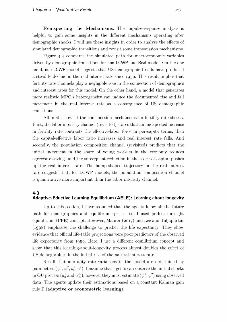
Using a monetary model I explore to which extent US demographicfactors have contributed to the observed rise and fall in the inflation rateduring 1950-2017. I have already shown that the dynamics in fertility rate andlife expectancy contributed with the rise and fall of the real interest rate in theperiod under analysis, however, there is a question I have not answered yet:how has the real interest dynamics affected monetary policy and inflation?
The answer to this questions relies on the way the central bank decideabout rit, i.e., the Taylor Rule Drift. As long as the central bank follows the

Chapter 4. Quantitative Results 32
Figure 4.5: Demographic Factors and Natural Interest Rate
Note. The dotted black line shows the variation in the real interest rate in a PFE’sworld, blue bars represent the contribution of fertility rate on interest rate movements, andwhite bars display the contribution of life expectancy variations. The dotted red line showsevolution of the real interest rate (deviations from the initial steady-state) in a AELE’smodel and light red bars display the contribution of learning-about-longevity process onthose variations. Shaded areas show 1960-1990 period.
variations implied for Natural model, i.e. rit = rNaturalt , then the inflation rate
would remain at zero for every moment. However, whenever the monetaryauthority does not internalize, or underestimate, the role of demographics onthe natural interest rate movements, then US demographic transitions canconsiderably affect inflation rate dynamics.
I assume that rit equals a smoothed path of the real interest rate along theperiod under analysis4. Next, I compare the simulation path to the effectivetrajectory for ex-ante real interest rate, nominal interest rate, and inflation. Inorder to obtain a reasonable measure of inflation expectations for the entiresample I estimated a time-varying first-order autorregression as in Hamiltonet al. (2016). Figure 4.6 plots Federal Funds Rate (FFR) and the return of 3-Months Treasury Bills (TB - 3M) in both nominal and ex-ante real terms. Allof these variables are characterize by a hump-shaped behaviour from 1950 to2017. Our model suggests that 1 percentage point of the rise in real interest ratefrom 1950 to the end-1970s is driven by demographic factors. Specifically, thetemporal increase in the share of young workers has generated a reduction insavings and produced an increase in the real interest rate during this period.Moreover, from the beginning of 1980s to the present, demographic factorshave contributed to the reduction of 3 percentage points in the real interestrate. For this period, both the reversion in the initial rise in fertility rate and
4It is roughly constant and equal to its initial steady-state value.
Chapter 4. Quantitative Results 33
the negative contribution of the increase in life expectancy explain this results.Finally, central bank’s miss-perception in the initial rise of the natural interestcan partially explain an inflationary episode of 2 percentage points. As long asthe natural interest rate declined, a disinflationary episode started. The modelsuggests that demographics have accounted for 2.5 p.p. of the reduction in theinflation rate since 1980.
Figure 4.6: Demographics, Real Interest Rate and Inflation
4.6(a): Real Interest Rate 4.6(b): Nominal Interest Rate
4.6(c): Inflation Rate
Note. Shaded areas show 1960-1990 period.

5Conclusion
I develop an overlapping generations model with life-cycle wage profile,age-dependent mortality rate, liquidity constraints, and nominal rigidities.The model is calibrated to capture the evolution of US demographics andother salient features of the US economy during 1950-2017. Then, I use themodel to study the role of demographic trends in explaining real interest ratemovements.
There are four main findings in this dissertation. First, I revisit theMPC’s heterogeneity channel and highlight it as a powerful transmissionmechanism for fertility rate variations. Since young workers are less productivethan middle-aged workers and they face liquidity constraints, the marginalpropensity to consume is higher for the former. Next, I find that this channelplays a major role in explaining the evolution of the real and natural interestrate. Specifically, I state that the rapid increase in working age populationfrom 1950-1980s have significantly contributed in the rise of real interest rates.The reversion of the fertility process together with the rise in life expectancytriggered a rapid decline in the natural interest rate since 1980s.
Thirdly, given the empirical evidence on large life expectancy forecastingerrors, I combine adaptive and eductive learning equilibrium concept and findthat the demographic contribution to the rise of the real and natural interestrate can be doubled due to learning-about-longevity process. Finally, sincedemographic trends affect aggregate saving rates and the natural interest rate,the failure to account for them might trigger inflationary (or deflationary)episodes. Hence, I remark that central banks’ miss-perception of the initialrise in the natural interest rate in the 1950s can potentially explain an initialinflationary episode, and, as long as the natural interest rate started declining,a disinflationary process.

Bibliography
Achdou, Y., Han, J., Lasry, J.-M., Lions, P.-L., and Moll, B. (2017). Incomeand wealth distribution in macroeconomics: A continuous-time approach.NBER Working Papers 23732, National Bureau of Economic Research, Inc.
Ahn, S., Kaplan, G., Moll, B., Winberry, T., and Wolf, C. (2017). Wheninequality matters for macro and macro matters for inequality. In NBER
Macroeconomics Annual 2017, volume 32. National Bureau of EconomicResearch, Inc.
Aksoy, Y., Basso, H., Grasl, T., and Smith, R. (2015). Demographic struc-ture and macroeconomic trends. Birkbeck Working Papers in Economicsand Finance 1501, Birkbeck, Department of Economics, Mathematics andStatistics.
Backus, D., Cooley, T., and Henriksen, E. (2013). Demography and lowfrequency capital flows. Working Paper 19465, National Bureau of EconomicResearch.
Bayo, F. (1966). United States Population Projections for OASDHI CostEstimates. Actuarial Studies Study 62, US Social Security.
Carvalho, C. and Ferrero, A. (2015). What explains japan’s persistentdeflation? 2013 Meeting Papers 1163, Society for Economic Dynamics.
Carvalho, C., Ferrero, A., and Nechio, F. (2016). Demographics and realinterest rates: Inspecting the mechanism. European Economic Review,88(C):208–226.
Clark, T. E. and Kozicki, S. (2005). Estimating equilibrium real interestrates in real time. The North American Journal of Economics and Finance,16(3):395–413.
Curtis, C., Lugauer, S., and Mark, N. (2017). Demographics and aggregatehousehold saving in japan, china, and india. Journal of Macroeconomics,51(C):175–191.

Bibliography 36
Curtis, C. C., Lugauer, S., and Mark, N. C. (2015). Demographic patterns andhousehold saving in china. American Economic Journal: Macroeconomics,7(2):58–94.
De Nardi, M. (2004). Wealth Inequality and Intergenerational Links. Review
of Economic Studies, 71(3):743–768.
De Nardi, M. and Yang, F. (2014). Bequests and heterogeneity in retirementwealth. European Economic Review, 72(C):182–196.
Del Negro, M., Giannone, D., Giannoni, M., and Tambalotti, A. (2017). Safety,liquidity, and the natural rate of interest. Staff Reports 812, Federal ReserveBank of New York.
Del Negro, M., Tambalotti, A., Giannone, D., and Giannoni, M. (2019). GlobalTrends in Interest Rates. Technical report.
Duffie, D. and Epstein, L. (1992). Stochastic differential utility. Econometrica,60(2):353–94.
Eusepi, S. and Preston, B. (2011). Expectations, Learning, and Business CycleFluctuations. American Economic Review, 101(6):2844–2872.
Evans, G. W. and Honkapohja, S. (2001). Learning and Expectations in
Macroeconomics. Princeton University Press.
Evans, G. W. and Honkapohja, S. (2009). Learning and Macroeconomics.Annual Review of Economics, 1(1):421–451.
Farhi, E. and Werning, I. (2017). Monetary Policy, Bounded Rationality,and Incomplete Markets. Working Paper 503421, Harvard UniversityOpenScholar.
Favero, C., Gozluklu, A. E., and Yang, H. (2016). Demographics and thebehavior of interest rates. IMF Economic Review, 64(4):732–776.
Ferrero, A. (2010). A structural decomposition of the U.S. trade balance: Pro-ductivity, demographics and fiscal policy. Journal of Monetary Economics,57(4):478–490.
Ferrero, G., Gross, M., and Neri, S. (2017). On secular stagnation and lowinterest rates: demography matters. Working Paper Series 2088, EuropeanCentral Bank.

Bibliography 37
Fiorentini, G., Galesi, A., Pérez-Quirós, G., and Sentana, E. (2018). Therise and fall of the natural interest rate. Working Papers 1822, Banco deEspaña;Working Papers Homepage.
Gertler, M. (1999). Government debt and social security in a life-cycleeconomy. Carnegie-Rochester Conference Series on Public Policy, 50(1):61–110.
Hall, R. (1988). Intertemporal substitution in consumption. Journal of
Political Economy, 96(2):339–57.
Hamilton, J. D., Harris, E. S., Hatzius, J., and West, K. D. (2016). TheEquilibrium Real Funds Rate: Past, Present, and Future. IMF Economic
Review, 64(4):660–707.
Holston, K., Laubach, T., and Williams, J. C. (2017). Measuring the naturalrate of interest: International trends and determinants. Journal of Interna-
tional Economics, 108(S1):59–75.
Hubbard, R. G. and Judd, K. L. (1986). Liquidity Constraints, Fiscal Policy,and Consumption. Brookings Papers on Economic Activity, 17(1):1–60.
Jappelli, T. (1990). Who is credit constrained in the u. s. economy? The
Quarterly Journal of Economics, 105(1):219–234.
Jappelli, T. and Pistaferri, L. (2010). The consumption response to incomechanges. Annual Review of Economics, 2(1):479–506.
Kaplan, G., Moll, B., and Violante, G. L. (2018). Monetary policy accordingto hank. American Economic Review, 108(3):697–743.
Lagakos, D., Moll, B., Porzio, T., Qian, N., and Schoellman, T. (2018).Life Cycle Wage Growth across Countries. Journal of Political Economy,126(2):797–849.
Lee, R. and Tuljapurkar, S. (1998). Population forecasting for fiscal planning:Issues and innovations. Working paper.
Lee, R. D. and Carter, L. R. (1992). Modeling and forecasting u.s. mortality.Journal of the American Statistical Association, 87(419):659–671.
Lunsford, K. G. and West, K. D. (2017). Some Evidence on Secular Driversof US Safe Real Rates. Working Papers (Old Series) 1723, Federal ReserveBank of Cleveland.

Bibliography 38
Maurer, T. (2017). Asset pricing implications of demographic change. Tech-nical report, 24th Australasian Finance and Banking Conference 2011.
Molavi, P. (2019). Macroeconomics with Learning and Misspecification: AGeneral Theory and Applications. Technical report.
Qiu, Z. (2018). Level-k dsge and monetary policy. SSRN Electronic Journal.
Rotemberg, J. (1982). Monopolistic price adjustment and aggregate output.Review of Economic Studies, 49(4):517–531.
Sudo, N. and Takizuka, Y. (2018). Population Aging and the Real InterestRate in the Last and Next 50 Years – A tale told by an OverlappingGenerations Model –. Bank of Japan Working Paper Series 18-E-1, Bank ofJapan.
Wade, A. (1989). Social Security Area Population Projections, 1989. ActuarialStudies Study 105, US Social Security.
Yogo, M. (2004). Estimating the elasticity of intertemporal substitution wheninstruments are weak. The Review of Economics and Statistics, 86(3):797–810.

ADerivation of the model
Here I present a derivation sketch of the non-linear system of partialdifferential equations which determines equilibrium in the model. First, Itransform the agent problem in a stationary problem. Second, I normalizethe cross-section distribution functions gi(). Finally, the government budgetconstraint is expressed in effective-labor units.
A.1Households
Worker. I adapt the method presented in Duffie and Epstein (1992)for specifying utility processes. With Possion compensated jump process, Iconjecture that Uw
t (j) has stochastic differential representation of the form
dUwt (j) = µwt (j)dt+ [V r
t (a, j)− Uwt (j)] dJrt (j) + [V (a)− Uw
t (j)] dJdt (j) (A-1)
where Jdt (j) and Jrt (j) are compensated Poisson processes with age-dependenthazard rate. The agent dies (retires) if Jdt (j) (Jrt (j)) jumps the first time sincethe agent is born. In the model, the arrival of death (retirement) is time-varying. Following Duffie and Epstein (1992), this implies
µwt (j) = −{u(cwt )− ρUw
t (j) + λrt (j)[V rt (a, j)− Uw
t (j)] + λdt (j)[V (a)− Uwt (j)]
}(A-2)
Since the state evolves according to Equation (2-5) and dj = dt, then thesolution to this problem is given by a value function V w
t (a, j) which satisfiesEquation (2-6).
Since there is exogenous productivity growth µxt , the HJB equation mustbe normalized by X1−1/η
t . Let V wt (a, j) = V wt (a,j)
X1−1/ηt
be the intermediate detrended
value function and Q = QXt
denotes the normalized value of variable Q. Thence
0 = maxc
u(c
Xt
)− ρV w
t (a, j) + ∂aVwt (a, j)swt (a, j) + ∂jV
wt (a, j)
+ λrt (j)[V rt (a, j)− V w
t (a, j)] + λdt (j)[V (a)− V wt (a, j)]

Appendix A. Derivation of the model 40
+ ∂tVwt (a, j) + µxt (1− 1/η)V w
t (a, j)
where swt (a, j) = rta + (1 − ςt)e(j)wt + e(j)Πt + ξt − τt − c and V (a) =φ1(a + φ2)1−1/η. This HJB equation is still non-stationary because there arepermanent changes in wt. To address it, I characterize the value function interms of a rather than in a itself. Define the final detrended value functionV wt (a, j) as V w
t (a, j) = V wt (a, j). I will guess that V w
t (a, j) does not depend onthe non-stationary variable Xt and then verify it. It is easy to compute
∂aVwt (a, j) = ∂aV
wt
(a
Xt
, j)
= 1Xt
∂aVwt (a, j)
∂jVwt (a, j) = ∂jV
wt (a, j)
∂tVwt (a, j) = ∂tV
wt
(a
Xt
, j)
= ∂tVwt (a, j)− µxt a∂aV w
t (a, j)
Substituting the intermediate value function by the final one, I obtain the HJB
stationary equation
0 = maxc
u (c)− ρV wt (a, j) + ∂aV
wt (a, j)swt (a, j) + ∂jV
wt (a, j)
+ λrt (j)[V rt (a, j)− V w
t (a, j)] + λdt (j)[V (a)− V wt (a, j)]
+ ∂tVwt (a, j) + µxt (1− 1/η)V w
t (a, j)
subject to a ≥ −a, where swt (a, j) = [rt−µxt ]a+(1−ςt)e(j)wt+e(j)Πt+ξt−τt−c.This HJB equation clearly does not depend on Xt. The first order conditionsfor this problem is
∂aVwt (a, j) = ∂cu(c) (A-3)
for any a, j. The state constraint implies a state-constraint boundary condition
∂aVwt (−a, j) ≥ ∂cu
(−[rt − µxt ]a+ (1− ςt)e(j)wt + e(j)Πt + ξt − τt
)(A-4)
for any j.
Retirees. Similarly, I can derive the HJB stationary equation for retirees
0 = maxc
u (c)− ρV rt (a, j) + ∂aV
rt (a, j)srt (a, j) + ∂jV
rt (a, j)

Appendix A. Derivation of the model 41
+ λdt (j)[V (a)− V rt (a, j)] + ∂tV
rt (a, j) + µxt (1− 1/η)V r
t (a, j)
subject to a ≥ −a, where srt (a, j) = [rt − µxt ]a + ξt + St − c. Hence, the firstorder condition for retiree’s problem is
∂aVrt (a, j) = ∂cu(c) (A-5)
for any a, j. The state constraint implies a state-constraint boundary condition
∂aVrt (−a, j) ≥ ∂cu
(−[rt − µxt ]a+ ξt + St
)(A-6)
for any j.
A.2Kolmogorov Forward Equation
The optimal decision rules of workers and retirees imply optimal drifts fortotal assets and, together with the exogenous aging process, they induce a jointdistribution of wealth and age, git(.). The evolution of this joint distribution isgiven by the Kolmogorov Forward (KF) equation:
∂tgwt (a, j) = −∂a[swt (a, j)gwt (a, j)]− ∂jgwt (a, j)− λwt (j)gwt (a, j) + δ(j)δ(a)btNw
t
∂tgrt (a, j) = −∂a[srt (a, j)grt (a, j)]− ∂jgrt (a, j)− λdt (j)grt (a, j) + λrt (j)gwt (a, j)
where swt and srt are the optimal drifts in assets implied by HJB equations,λwt (j) equals λrt (j) + λdt (j), and δ(.) is the Dirac delta function. Again, I mustnormalize these distributions. Let git(a, j) be the same measures but in termsof a instead of a, then I can directly construct the KF equations for them
∂tgwt (a, j) = −∂a[swt (a, j)gwt (a, j)]− ∂j gwt (a, j)− λwt (j)gwt (a, j) + δ(j)δ(a)btNw
t
∂tgrt (a, j) = −∂a[srt (a, j)grt (a, j)]− ∂j grt (a, j)− λdt (j)grt (a, j) + λrt (j)gwt (a, j)
Note that∫ ∫
gwt (a, j)dadj = Nwt plus
∫ ∫grt (a, j)dadj = N r
t equals Nt. Hence,let git(a, j) = git(a,j)
Ntbe the normalized measures of workers and retirees which
follow
∂tgwt (a, j) = −∂a[swt (a, j)gwt (a, j)]− ∂j gwt (a, j)− [λwt (j) + nt]gwt (a, j) + δ(j)δ(a)bt
Nwt
Nt
∂tgrt (a, j) = −∂a[srt (a, j)grt (a, j)]− ∂j grt (a, j)− [λdt (j) + nt]grt (a, j) + λrt (j)gwt (a, j)

Appendix A. Derivation of the model 42
A.3Analysis
Here, I report some analytical results of the model. Specifically, I aminterested in both deriving the stationary age distribution of the model andthe evolution of it. Computing age-distributions outside the system describedin Appendix B is extremely helpful in finding the competitive equilibrium.
Worker Population. Let Nwt (j) be the number of workers aged j years
at t, then worker population grows according to
dNwt = btN
wt dt−
[∫ ∞0
λwt (j)Nwt (j)dj
]dt (A-7)
Retiree Population. Similarly, let N rt (j) be the number of retirees aged
j years at t, henceforth
dN rt =
[∫ ∞0
λrt (j)Nwt (j)dj
]dt−
[∫ ∞0
λdt (j)N rt (j)dj
]dt (A-8)
Age Distribution. Contrary to wealth distribution, in the model theage distribution is determined exogenously. These measures only depend onexogenous processes {bt, λrt (j), λrt (j)} and I make some further analysis forfinding the stationary version of them. The main conclusions of this analysiscan be summarized in
1. The number of workers at age j can be calculated by
Nwt (j) = bt−jN
wt−je
−∫ j
0 λwt−j+v(v)dv (A-9)
where λwt (j) = λrt (j) + λdt (j).
2. Let N rt (j, s) be the number of retirees aged j years with s ∈ (0, j] years
in retirement, hence
N rt (j, s) = λrt−s(j − s)Nw
t−s(j − s)e−∫ s
0 λdt−s+v(j−s+v)dv (A-10)
Furthermore, N rt (j) =
∫ j0 N
rt (j, s)ds and N r
t =∫∞
0 N rt (j)dj.
3. At any stationary equilibrium the measure of workers, retirees, and totalpopulation grows at the same rate n = nw = nr. Moreover, let Si(j) thesurvival function for the compensated Poisson process J i(j), then n isdetermined by
n = b[1−
∫ ∞0
λw(j)Sw(j)e−njdj]
(A-11)
(A-12)

Appendix A. Derivation of the model 43
4. Finally, the stationary age distribution is
Nt(j)Nt
= Nt(j)Nwt
/∫ ∞0
Nt(j)Nwt
dj (A-13)
where Nt(j)Nwt
= Nwt (j)Nwt
+ Nrt (j)Nwt
and
Nwt (j)Nwt
= be−njSw(j) (A-14)
N rt (j)Nwt
= be−njSd(j)∫ j
0λr(v)S
w(v)Sd(v) dv (A-15)
A.4Firms and Government
For the remaining of this appendix Q = QXtNt
denotes per-capita variableswhile Q = Q
XtLtcharacterizes variables Q - efficiency labor rate.
Firms. Cost minimization implies
wtXt
= αmtyt,iXtlt,i
rt + δ = (1− α)mtyt,ikt,i
Since every firm uses the same capital-efficiency labor ratio, aggregation issimple: Yt = K1−α
t [XtLt]α, then
Yt = K1−αt
wt = αmtK1−αt
rt + δ = (1− α)mtK−αt
Note that factor prices depend only on capital-efficiency labor ratio kt. Per-capita variables are given by
Y t = YtLtNt
Kt = KtLtNt
Furthermore, using YtYt
= Y tY t− Xt
Xt− Nt
Nt, I can rewrite the NK Phillips Curve in
terms of per-capita variables
Appendix A. Derivation of the model 44
πt =rt + µxt + nt −
Y t
Y t
πt − ε
θ(mt −m∗) (A-16)
Government. Normalize Equation (2-12) and obtain
Bt = [rt − µxt − nt]Bt +Gt −Nwt
Nt
τt
Using fiscal rules: Bt = byYt and Gt = gyYt,
Bt = [(rt − µxt − nt)by + gy]K1−αt
LtNt
− Nwt
Nt
τt
or, equivalently
τt =(Nwt
Nt
)−1 ([(rt − µxt − nt)by + gy]K1−α
t
LtNt
− Bt
)(A-17)
Finally, social security and bequests can be normalized as follows:
St = ςtwtLtN rt
(A-18)
ξt =∫ ∞
0λdt (j)
∑i∈{w,r}
∫agit(a, j)da
dj (A-19)

BCompetitive Equilibrium
0 = maxc
u (c)− ρV wt (a, j) + ∂aV
wt (a, j)swt (a, j) + ∂jV
wt (a, j)
+ λrt (j)[V rt (a, j)− V w
t (a, j)] + λdt (j)[V (a)− V wt (a, j)]
+ µxt (1− 1/η)V wt (a, j) + ∂tV
wt (a, j)
(B-1)
0 = maxc
u (c)− ρV rt (a, j) + ∂aV
rt (a, j)srt (a, j)
+ ∂jVrt (a, j) + λdt (j)[V (a)− V r
t (a, j)]
+ µxt (1− 1/η)V rt (a, j) + ∂tV
rt (a, j)
(B-2)
0 = −∂tgwt (a, j)− ∂a[swt (a, j)gwt (a, j)]− ∂j gwt (a, j)
− [λwt (j) + nt]gwt (a, j) + δ(j)δ(a)btNwt
Nt
(B-3)
0 = −∂tgrt (a, j)− ∂a[srt (a, j)grt (a, j)]− ∂j grt (a, j)
− [λdt (j) + nt]grt (a, j) + λrt (j)gwt (a, j) (B-4)
Yt = K1−αt (B-5)
wt = αmtK1−αt (B-6)
rt = (1− α)mtK−αt − δ (B-7)
Y t = YtLtNt
(B-8)
Kt = KtLtNt
(B-9)
0 = ε
θ(mt −m∗) + πt −
rt + µxt + nt −Y t
Y t
πt (B-10)
Πt =(
1−mt −θ
2π2t
)K1−αt
LtNt
(B-11)
Bt = [(rt − µxt − nt)by + gy]K1−αt
LtNt
− Nwt
Nt
τt (B-12)
St = ςtwtLtN rt
(B-13)

Appendix B. Competitive Equilibrium 46
ξt =∫ ∞
0λdt (j)
∑i∈{w,r}
∫agit(a, j)da
dj (B-14)
0 =∑
i∈{w,r}
∫ ∫agit(a, j)dadj −
[Kt +Bt
](B-15)
where
swt (a, j) = [rt − µxt ]a+ (1− ςt)e(j)wt + e(j)Πt + ξt − τt − cwt (a, j)
srt (a, j) = [rt − µxt ]a+ ξt + St − c
Bt = byY t
Gt = gyY t

CNumeric Algorithm
I explain the numeric algorithm in two parts. I start explaining howto compute the stationary equilibrium and then how to calculate transitiondynamics.
C.1Stationary Equilibrium
HJB equation. Based on Achdou et al. (2017) and Ahn et al. (2017), Iuse implicit methods and upwind scheme. Let ∆ ∈ R+, then for a given gridin asset and age, i ∈ {1, . . . , I} and j ∈ {1, . . . , J}, the HJB equation becomes
vn+1w (i, j)− vnw(i, j)
∆ = u(cnw(i, j))− ρwvn+1w (i, j) + λr(j)vn+1
r (i, j) + λd(j)V (i)
+ ∂avn+1w (i, j)snw(i, j) + ∂jv
n+1w (i, j)
vn+1r (i, j)− vnr (i, j)
∆ = u(cnr (i, j))− ρrvn+1r (i, j) + λd(j)V (i)
+ ∂avn+1w (i, j)snw(i, j) + ∂jv
n+1w (i, j)
where ρw = ρ+ λw(j)− µx(1− 1/η) and ρr = ρ+ λd(j)− µx(1− 1/η).Stacking {vr(i, j); vw(i, j)} in the vector v and {cr(i, j); cw(i, j)} in the
vector cvn+1 − vn
∆ = u(c) + v + xvn+1 + Anvn+1 + Cvn+1
where x groups ρk, An is related to saving decisions, and C associated to theageing process. In order to solve the HJB equation by implicit method I iterate
vn+1 = (1/∆− x−An −C)−1[u(c) + v + vn
∆
](C-1)
until convergence.
KF equation. Let A = limn→∞An and g be the stacked version of{gr(i, j); gw(i, j)}, then from FK equation I obtain
0 = ATg + Bg + b

Appendix C. Numeric Algorithm 48
where B is a matrix related to the ageing process and b characterizesthe Dirac function in KF equation, hence
g = −[AT + B]−1b (C-2)
Algorithm. The algorithm to compute the stationary equilibrium issimple.
1. Guess K.
2. Calculate implied prices:
m? = ε− 1ε
r = (1− α)m?K−α − δkw = αm?K1−α
3. Calculate implied profits
Π = (1−m?)K1−α = 1εK1−α L
N
4. Compute fiscal policy
τ = [(r − µx − n)by + gy]K1−α L
Nw
5. Solve household’s problem for both retirees and workers: eq. (C-1) andeq. (C-2).
6. Calculate aggregate asset demand: A, and the aggregate asset supply:
As =
(K + byK
1−α) LN
7. Compute excess demand:
Λ = |As − A|
8. If Λ is close to zero the equilibrium have been found. Otherwise updatethe guess and go back to step 2.

Appendix C. Numeric Algorithm 49
C.2Transition Dynamics
A similar algorithm can be used the economy’s impulse response after anunanticipated (zero probability) shock followed by a deterministic transition.
HJB dynamic equation. Using previous notation, I can solve vt usingthe dynamic HJB equation and a terminal condition vT = limn→∞ vn,
vt−1 − vt∆t = u(ct) + v + xtvt + Atvt + Cvt
where x and A are now time-dependent, thus, from t = T, . . . , 1, I compute
vt−1 = (1/∆− xt −At −C)−1[u(ct) + v + vt
∆t
](C-3)
KF dynamic equation. Given an initial condition g0 = g and the KFequation, I can solve for {gt}
gt+1 − gt∆t = AT
t gt+1 + Btgt+1 + bt
hence,
gt+1 =[I−∆t
(ATt + Bt
)]−1[gt + ∆tbt] (C-4)
Algorithm. The algorithm to calculate the transition dynamics is
1. Compute the stationary equilibrium (initial s0 and final sf).
2. Guess a path for interest rate, {rt}T0 .
3. Using Taylor equation forwardly in time, π−1 = 0, solve for inflation rate
dπtdt
= −θi[it − rit − φππt]−drtdt
4. Using Phillips Curve backward in time (with mT = m∗) and marginalcost equation I must solve,
mt = m? + θ
ε
rt − (1− α)˙Kt
Kt
− µxt − nwt
πt − πt
Kt =[
rt + δk(1− α)mt
]−1/α

Appendix C. Numeric Algorithm 50
5. Compute wages and profits
wt = αmtK1−αt
Πt =(
1−mt −θ
2π2t
)K1−αt
6. Find fiscal taxes by
Bt = byK1−αt
LtNt
τt =(Nwt
Nt
)−1 ([(rt − µxt − nt)by + gy
]K1−αt
LtNt
− Bt
)
7. Solve household’s problem using eq. (C-3) and eq. (C-4).
8. Compute aggregate demand At and supply A. Calculate excess demand
Λt = |Ast − At|
9. If, for all t, Λt is close to zero, then the equilibrium have been found.Otherwise update the guess and go back to step 2.

DAdaptive-Eductive Learning Equilibrium - AELE
In this chapter, I explain the learning equilibrium concept used in Sec-tion 4.3. It is worth emphasizing that I present it as general as possible, thenit can be used in other kind of Heterogeneous Agent (HA) models.1
Exogenous System. Let xt be a vector of exogenous process and utinnovations over it, then assume that I can express the dynamics for this vectoras a system of linear differential equations
0 = Φ0dxtdt + Φ1xt + ut (D-1)
where ut is a vector of shocks. For instance, in the above model xt containsproductivity growth and demographic variables and I approximate the func-tions over a discretized grid of ages J = {j1 = 0, j2, . . . , jJ} in order to obtainthe representation of Equation (D-1).
Endogenous System. The endogenous part of any system consist ofa vector of value functions vt, a vector of distributions gt, a vector of policyinstruments ht, and a vector of prices pt. Thus, the endogenous system aredetermined by:
[HJB equations] 0 = U(vt) + A(vt; pt,ht,xt) + dvt
dt (D-2)
[KF equations] dgt
dt = G(vt; pt,ht,xt)gt (D-3)
[Policy equations] dhtdt = H(gt; pt,ht,xt) (D-4)
[Clearing Market Cond.] pt = P(gt; ht,xt) (D-5)
I also approximate the value function and distribution over a dis-cretized grid of asset holdings A = {a1 = −a, a2, . . . , aI}. Hence, de-note the value function and distribution along the discrete state-spaceA × J using vectors vt = [(V w
t (a, j))a∈A,j∈J , (V rt (a, j))a∈A,j∈J ]′ and
1Recent studies introduce bounded rationality in HA models to examine the role ofMonetary Policy within this framework. See Farhi and Werning (2017), Qiu (2018), andMolavi (2019).

Appendix D. Adaptive-Eductive Learning Equilibrium - AELE 52
gt = [(gwt (a, j))a∈A,j∈J , (grt (a, j))a∈A,j∈J ]′.
Point-wise Constrained Foresight Equilibrium (PCFE). Taking{xet,s}s≥t with xet,t = xt and {gs,ps,hs}s<t, the point-wise constrained foresight
equilibrium (PCFE) is given by the solution {vt,s,gt,s,pt,s,ht,s}s≥t of thefollowing system:
0 = U(vt,s) + A(vt,s; pt,s,ht,s,xet,s) + dvt,s
ds (D-6)dgt,s
ds = G(vt,s; pt,s,ht,s,xet,s)gt,s (D-7)
dht,sds = H(gt,s; pt,s,ht,s,xe
t,s) (D-8)
pt,s = P(gt,s; ht,s,xet,s) (D-9)
Adaptive-Eductive Learning Equilibrium (AELE). The equilib-rium concept used in Section 4.3 combines adaptive or econometric learn-ing equilibrium2 (about exogenous system) and PCFE (for the endogenoussystem).
First, I assume that expectations about exogenous vector xt are recur-sively updated as in Least-Square Econometric Learning models. In this en-vironment, agents know the entire path of exogenous shocks {ut}t≥0 but notthe parameters governing the Data Generator Process (DGP). That is, theyshould learn about {Φ0,Φ1}. Then, given {xs}s≤t, they estimate {Φ0,Φ1} andforecast x based on their Perceived Law of Motion (PLM),
0 = Φ0,tdxet,sds + Φ1,txet,s + us (D-10)
for all s > t. In this document, I use a traditional updating rule based on aconstant Kalman gain Γi
dΦi,t = −Γi[Φi,t −Φi,t]dt (D-11)
for i ∈ {1, 2}.Secondly, at any moment and given expectations on exogenous variables
{xet,s}s>t at t, expectations about {gt, pt, ht} are formed eductively. Hence, Idefine Adaptive-Eductive Learning Equilibrium (AELE) concept as acontinuous sequence of PCFE {{vt,s,gt,s,pt,s,ht,s,nt,s}s≥t}t≥0 consistent withLeast-Square learning expectations {xet,s}s≥t with xet,t = xt for every t.
2See for example Evans and Honkapohja (2001), Evans and Honkapohja (2009), andEusepi and Preston (2011).

Appendix D. Adaptive-Eductive Learning Equilibrium - AELE 53
Redefining Perfect Foresight Equilibrium (PFE). PFE assumesthat agents know the trajectory of the unexpected shock {ut} and the DGPfor exogenous process, i.e., Φ1,t = Φ1 and Φ0,t = Φ0 for all t. Hence,thePFE can be redefined as a sequence of PCFE {{vt,s,gt,s,pt,s,ht,s,nt,s}s≥t}t≥0
consistent with true exogenous DGP process {xet,s = xs}s≥t for every t.