UFABC - Física Quântica - Curso 2017.3 Prof. Germán Lugones

Aula 3 Espectros atômicos e modelo atômico de

Rutherford

1

Uma versão de alta resolução do espectro do nosso Sol. Cada uma das 50 faixas cobre 60 angstroms. O espectro completo corresponde ao intervalo de luz visível entre 4000 e 7000 angstroms.

Espectros atômicos

2

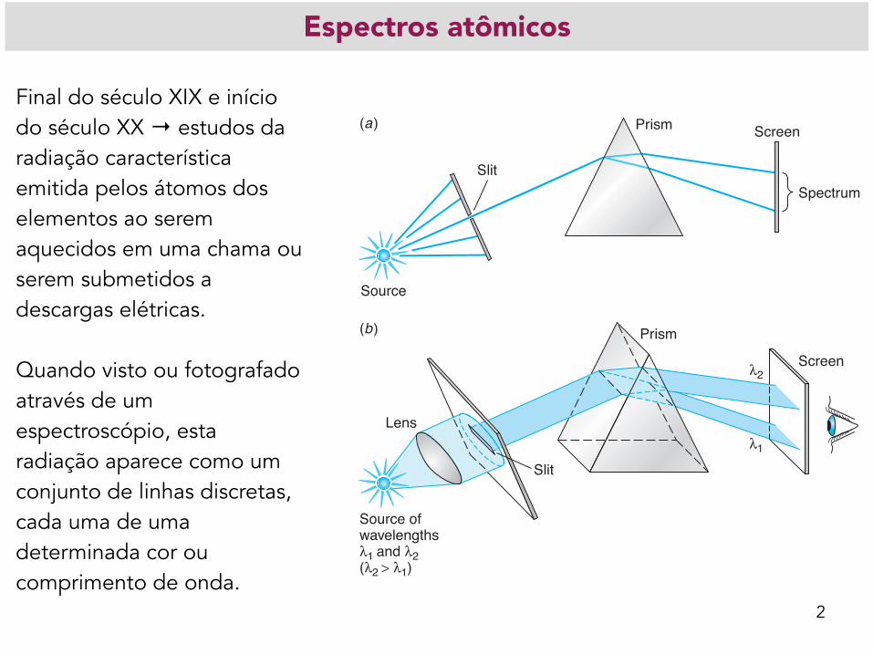
Final do século XIX e início do século XX → estudos da radiação característica emitida pelos átomos dos elementos ao serem aquecidos em uma chama ou serem submetidos a descargas elétricas.

Quando visto ou fotografado através de um espectroscópio, esta radiação aparece como um conjunto de linhas discretas, cada uma de uma determinada cor ou comprimento de onda.

154 Chapter 4 The Nuclear Atom

exist. Explaining the origin of the sharp lines and accounting for the primary features of the spectrum of hydrogen, the simplest element, was a major success of the so-called old quantum theory begun by Planck and Einstein and will be the main topic in this chapter. Full explanation of the lines and bands requires the later, more sophisticated quantum theory, which we will begin studying in Chapter 5.

4-1 Atomic Spectra The characteristic radiation emitted by atoms of individual elements in a flame or in a gas excited by an electrical discharge was the subject of vigorous study during the late nineteenth and early twentieth centuries. When viewed or photographed through a spectroscope, this radiation appears as a set of discrete lines, each of a particular color or wavelength; the positions and intensities of the lines are characteristic of the element. The wavelengths of these lines could be determined with great precision,

Source ofwavelengths�1 and �2(�2 � �1)

�1

�2

Slit

Lens

Source

Prism

Screen

Slit

Prism Screen

Spectrum

(a)

(b)

FIGURE 4-1 (a) Light from the source passes through a small hole or a narrow slit before falling on the prism. The purpose of the slit is to ensure that all the incident light strikes the prism face at the same angle so that the dispersion by the prism causes the various frequencies that may be present to strike the screen at different places with minimum overlap. (b) The source emits only two wavelengths, L2 � L1. The source is located at the focal point of the lens so that parallel light passes through the narrow slit, projecting a narrow line onto the face of the prism. Ordinary dispersion in the prism bends the shorter wavelength through the larger total angle, separating the two wavelengths at the screen. In this arrangement each wavelength appears on the screen (or on CCD detectors replacing the screen) as a narrow line, which is an image of the slit. Such a spectrum was dubbed a “line spectrum” for that reason. Prisms have been almost entirely replaced in modern spectroscopes by diffraction gratings, which have much higher resolving power.

TIPLER_04_153-192hr.indd 154 8/22/11 11:36 AM

3

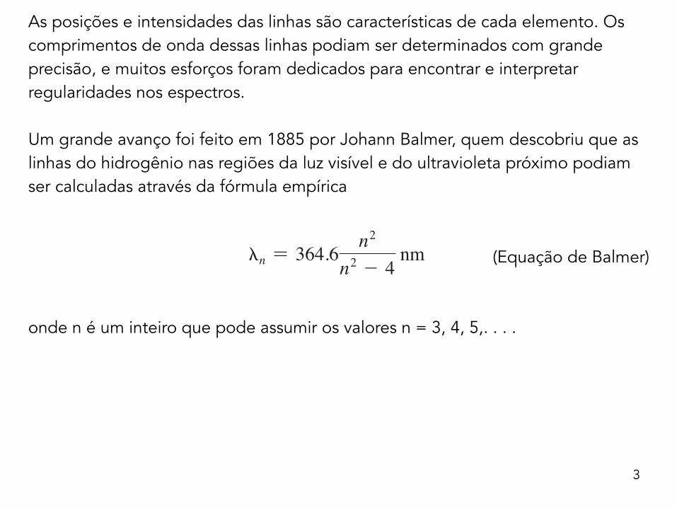
As posições e intensidades das linhas são características de cada elemento. Os comprimentos de onda dessas linhas podiam ser determinados com grande precisão, e muitos esforços foram dedicados para encontrar e interpretar regularidades nos espectros.

Um grande avanço foi feito em 1885 por Johann Balmer, quem descobriu que as linhas do hidrogênio nas regiões da luz visível e do ultravioleta próximo podiam ser calculadas através da fórmula empírica

(Equação de Balmer)

onde n é um inteiro que pode assumir os valores n = 3, 4, 5,. . . .

4-1 Atomic Spectra 155

and much effort went into finding and interpreting regularities in the spectra. A major breakthrough was made in 1885 by a Swiss schoolteacher, Johann Balmer, who found that the lines in the visible and near ultraviolet spectrum of hydrogen could be repre-sented by the empirical formula

Ln � 364.6n2

n2 � 4 nm 4-1

where n is a variable integer that takes on the values n � 3, 4, 5, . . . . Figure 4-2a is a photo of the set of spectral lines of hydrogen (now known as the Balmer series) whose wavelengths are given by Balmer’s formula. For example, the wavelength of the HA line could be found by letting n � 3 in Equation 4-1 (try it!), and other integers each predicted a line that was found in the spectrum. Balmer suggested that his formula might be a special case of a more general expression applicable to the spectra of other elements when ionized to a single electron, that is, hydrogenlike elements. Such an

The uniqueness of the line spectra of the elements has enabled astronomers to determine the composition of stars, chemists to identify unknown compounds, and theme parks and entertainers to have laser shows.

FIGURE 4-2 (a) Emission line spectrum of hydrogen in the visible and near ultraviolet. The lines appear dark because the spectrum was photographed; hence, the bright lines are exposed (dark) areas on the film. The names of the first five lines are shown, as is the point beyond which no lines appear, H@, called the limit of the series. (b) A portion of the emission spectrum of sodium. The two very close bright lines at 589 nm are the D1 and D2 lines. They are the principal radiation from sodium street lighting. (c) A portion of the emission spectrum of mercury. (d ) Part of the dark line (absorption) spectrum of sodium. White light shining through sodium vapor is absorbed at certain wavelengths, resulting in no exposure of the film at those points. Notice that the line at 259.4 nm is visible here in both the bright and dark line spectra. Note that frequency increases toward the right, wavelength toward the left in the four spectra shown.

Hydrogen

(a)

Sodium

(b)

Mercury

(c)

656.3

D1

D2

588.9

589.5

330.3

546.1

435.8

253.6

285.3

268.0

259.4

486.1

434.0

410.2

397.0

389.0

364.6

H� H� H� H� H� f

Sodium

(d )

259.4

254.4

251.2

f

f

f

H�

TIPLER_04_153-192hr.indd 155 8/22/11 11:36 AM

A Figura é uma foto do conjunto de linhas espectrais de emissão do hidrogênio (agora conhecido como a série Balmer).

• As linhas aparecem na região da luz visível e no ultravioleta próximo. • As linhas aparecem escuras porque o espectro foi fotografado; portanto, as

linhas brilhantes são áreas expostas (escuras) no filme. • Se mostram os nomes das primeiras cinco linhas, assim como o ponto além do

qual nenhuma linha aparece, H∞, chamado limite da série.

- Os comprimentos de onda são dados pela fórmula de Balmer. - Por exemplo, o comprimento de onda da linha H𝛼 pode ser encontrado usando

n=3 na Equação de Balmer (verifique!) - As outras linhas correspondiam a outros valores inteiros de n. - O limite da série é obtido usando n=∞. 4

4-1 Atomic Spectra 155

and much effort went into finding and interpreting regularities in the spectra. A major breakthrough was made in 1885 by a Swiss schoolteacher, Johann Balmer, who found that the lines in the visible and near ultraviolet spectrum of hydrogen could be repre-sented by the empirical formula

Ln � 364.6n2

n2 � 4 nm 4-1

where n is a variable integer that takes on the values n � 3, 4, 5, . . . . Figure 4-2a is a photo of the set of spectral lines of hydrogen (now known as the Balmer series) whose wavelengths are given by Balmer’s formula. For example, the wavelength of the HA line could be found by letting n � 3 in Equation 4-1 (try it!), and other integers each predicted a line that was found in the spectrum. Balmer suggested that his formula might be a special case of a more general expression applicable to the spectra of other elements when ionized to a single electron, that is, hydrogenlike elements. Such an

The uniqueness of the line spectra of the elements has enabled astronomers to determine the composition of stars, chemists to identify unknown compounds, and theme parks and entertainers to have laser shows.

FIGURE 4-2 (a) Emission line spectrum of hydrogen in the visible and near ultraviolet. The lines appear dark because the spectrum was photographed; hence, the bright lines are exposed (dark) areas on the film. The names of the first five lines are shown, as is the point beyond which no lines appear, H@, called the limit of the series. (b) A portion of the emission spectrum of sodium. The two very close bright lines at 589 nm are the D1 and D2 lines. They are the principal radiation from sodium street lighting. (c) A portion of the emission spectrum of mercury. (d ) Part of the dark line (absorption) spectrum of sodium. White light shining through sodium vapor is absorbed at certain wavelengths, resulting in no exposure of the film at those points. Notice that the line at 259.4 nm is visible here in both the bright and dark line spectra. Note that frequency increases toward the right, wavelength toward the left in the four spectra shown.

Hydrogen

(a)

Sodium

(b)

Mercury

(c)

656.3

D1

D2

588.9

589.5

330.3

546.1

435.8

253.6

285.3

268.0

259.4

486.1

434.0

410.2

397.0

389.0

364.6

H� H� H� H� H� f

Sodium

(d )

259.4

254.4

251.2

f

f

f

H�

TIPLER_04_153-192hr.indd 155 8/22/11 11:36 AM

Outros elementos químicos também apresentavam linhas de emissão:

5

4-1 Atomic Spectra 155

and much effort went into finding and interpreting regularities in the spectra. A major breakthrough was made in 1885 by a Swiss schoolteacher, Johann Balmer, who found that the lines in the visible and near ultraviolet spectrum of hydrogen could be repre-sented by the empirical formula

Ln � 364.6n2

n2 � 4 nm 4-1

where n is a variable integer that takes on the values n � 3, 4, 5, . . . . Figure 4-2a is a photo of the set of spectral lines of hydrogen (now known as the Balmer series) whose wavelengths are given by Balmer’s formula. For example, the wavelength of the HA line could be found by letting n � 3 in Equation 4-1 (try it!), and other integers each predicted a line that was found in the spectrum. Balmer suggested that his formula might be a special case of a more general expression applicable to the spectra of other elements when ionized to a single electron, that is, hydrogenlike elements. Such an

The uniqueness of the line spectra of the elements has enabled astronomers to determine the composition of stars, chemists to identify unknown compounds, and theme parks and entertainers to have laser shows.

FIGURE 4-2 (a) Emission line spectrum of hydrogen in the visible and near ultraviolet. The lines appear dark because the spectrum was photographed; hence, the bright lines are exposed (dark) areas on the film. The names of the first five lines are shown, as is the point beyond which no lines appear, H@, called the limit of the series. (b) A portion of the emission spectrum of sodium. The two very close bright lines at 589 nm are the D1 and D2 lines. They are the principal radiation from sodium street lighting. (c) A portion of the emission spectrum of mercury. (d ) Part of the dark line (absorption) spectrum of sodium. White light shining through sodium vapor is absorbed at certain wavelengths, resulting in no exposure of the film at those points. Notice that the line at 259.4 nm is visible here in both the bright and dark line spectra. Note that frequency increases toward the right, wavelength toward the left in the four spectra shown.

Hydrogen

(a)

Sodium

(b)

Mercury

(c)

656.3

D1

D2

588.9

589.5

330.3

546.1

435.8

253.6

285.3

268.0

259.4

486.1

434.0

410.2

397.0

389.0

364.6

H� H� H� H� H� f

Sodium

(d )

259.4

254.4

251.2

f

f

f

H�

TIPLER_04_153-192hr.indd 155 8/22/11 11:36 AM

6

Balmer sugeriu que sua fórmula poderia ser um caso especial de uma expressão mais geral aplicável aos espectros de outros elementos.

Tal expressão, foi encontrada de forma independente por J. R. Rydberg e W. Ritz e por isso é chamada de fórmula de Rydberg-Ritz,

onde m e n são números inteiros e R, a constante de Rydberg, é a mesma para todas as linhas do espectro de um elemento e varia apenas ligeiramente, e de forma regular, de elemento para elemento.

Para o hidrogênio, o valor de R é RH=1.096776×107 m-1. Para elementos muito pesados, R se aproxima para o valor limite R∞=1.097373×107 m-1.

Essas expressões empíricas foram bem sucedidas na predição de outras séries de linhas espectrais ainda não conhecidas, como as linhas do hidrogênio fora do espectro visível.

156 Chapter 4 The Nuclear Atom

expression, found independently by J. R. Rydberg and W. Ritz and thus called the Rydberg-Ritz formula, gives the reciprocal wavelength3 as

1

Lmn� R4 1

m2 � 1n2 5 for n � m 4-2

where m and n are integers and R, the Rydberg constant, is the same for all series of spectral lines of the same element and varies only slightly, and in a regular way, from element to element. For hydrogen, the value of R is RH � 1.096776 � 107 m�1. For very heavy elements, R approaches the value of R@ � 1.097373 � 107 m�1. Such empirical expressions were successful in predicting other series of spectral lines, such as other hydrogen lines outside the visible region.

EXAMPLE 4-1 Hydrogen Spectral Series The hydrogen Balmer series recip-rocal wavelengths are those given by Equation 4-2 with m � 2 and n � 3, 4, 5, . . . .For example, the first line of the series, HA, would be for m � 2, n � 3:

1L23

� R4 122 � 1

32 5 �536

R � 1.523 � 106 m�1

or

L23 � 656.5 nm

Other series of hydrogen spectral lines were found for m � 1 (by Lyman) and m � 3 (by Paschen). Compute the wavelengths of the first lines of the Lyman and Paschen series.

SOLUTIONFor the Lyman series (m � 1), the first line is for m � 1, n � 2.

1

L12� R4 1

12 � 122 5 �

34

R � 8.22 � 106 m�1

L12 � 121.6 nm �in the ultraviolet�For the Paschen series (m � 3), the first line is for m � 3, n � 4.

1

L34� R4 1

32 � 142 5 �

7144

R � 5.332 � 105 m�1

L34 � 1876 nm �in the infrared�All of the lines predicted by the Rydberg-Ritz formula for the Lyman and Paschen series are found experimentally. Note that no lines are predicted to lie beyond L@ � 1�R � 91.2 nm for the Lyman series and L@ � 9�R � 820.6 nm for the Paschen series and none are found by experiments.

4-2 Rutherford’s Nuclear Model Many attempts were made to construct a model of the atom that yielded the Balmer and Rydberg-Ritz formulas. It was known that an atom was about 10�10 m in diameter (see Problem 4-6), that it contained electrons much lighter than the atom (see Section 3-1), and that it was electrically neutral. The most popular model was J. J. Thomson’s model, already quite successful in explaining chemical reactions. Thomson attempted

TIPLER_04_153-192hr.indd 156 8/22/11 11:36 AM

7

No final do século XIX sabia-se que um átomo tinha cerca de 10-10m de diâmetro, que continha elétrons muito mais leves do que o átomo como um todo, e que ele era eletricamente neutro.

O problema era construir um modelo do átomo que, além de satisfazer todos esses requisitos, fosse compatível com as fórmulas de Balmer e Rydberg.

O modelo mais popular era o modelo de J. J. Thomson. Nesse modelo, os elétrons de carga negativa, estão distribuídos uniformemente num volume esférico contínuo de carga positiva.

O modelo nuclear de Rutherford

4-2 Rutherford’s Nuclear Model 157

various models consisting of electrons embedded in a fluid that contained most of the mass of the atom and had enough positive charge to make the atom electrically neu-tral (see Figure 4-3a). He then searched for configurations that were stable and had normal modes of vibration corresponding to the known frequencies of the spectral lines. One difficulty with all such models was that electrostatic forces alone cannot produce stable equilibrium. Thus, the charges were required to move and, if they stayed within the atom, to accelerate; however, the acceleration would result in con-tinuous emission of radiation, which is not observed. Despite elaborate mathematical calculations, Thomson was unable to obtain from his model a set of frequencies of vibration that corresponded with the frequencies of observed spectra.

The Thomson model of the atom was replaced by one based on the results of a set of experiments conducted by Ernest Rutherford4 and his students H. W. Geiger andE. Marsden. Rutherford was investigating radioactivity and had shown that the radia-tions from uranium consisted of at least two types, which he labeled A and B. He showed, by an experiment similar to that of J. J. Thomson, that q�m for the A was half that of the proton. Suspecting that the A particles were doubly ionized helium, Ruther-ford and his coworkers in a classic experiment let a radioactive substance A decay in a previously evacuated chamber; then, by spectroscopy, they detected the spectral lines of ordinary helium gas in the chamber. Realizing that this energetic, massive A particle

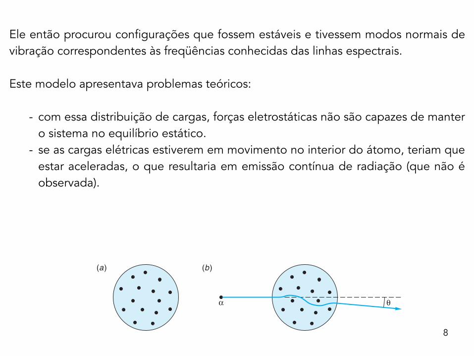
FIGURE 4-3 Thomson’s model of the atom: (a) A sphere of positive charge with electrons embedded in it so that the net charge would normally be zero. The atom shown would have been phosphorus. (b) An A particle scattered by such an atom would have a scatteringangle U much smaller than 1�.

(a) (b)

� �

Hans Geiger and Ernest Rutherford in their Manchester laboratory. [Courtesy of University of Manchester.]

TIPLER_04_153-192hr.indd 157 8/22/11 11:36 AM

8

Ele então procurou configurações que fossem estáveis e tivessem modos normais de vibração correspondentes às freqüências conhecidas das linhas espectrais.

Este modelo apresentava problemas teóricos:

- com essa distribuição de cargas, forças eletrostáticas não são capazes de manter o sistema no equilíbrio estático.

- se as cargas elétricas estiverem em movimento no interior do átomo, teriam que estar aceleradas, o que resultaria em emissão contínua de radiação (que não é observada).

4-2 Rutherford’s Nuclear Model 157

various models consisting of electrons embedded in a fluid that contained most of the mass of the atom and had enough positive charge to make the atom electrically neu-tral (see Figure 4-3a). He then searched for configurations that were stable and had normal modes of vibration corresponding to the known frequencies of the spectral lines. One difficulty with all such models was that electrostatic forces alone cannot produce stable equilibrium. Thus, the charges were required to move and, if they stayed within the atom, to accelerate; however, the acceleration would result in con-tinuous emission of radiation, which is not observed. Despite elaborate mathematical calculations, Thomson was unable to obtain from his model a set of frequencies of vibration that corresponded with the frequencies of observed spectra.

The Thomson model of the atom was replaced by one based on the results of a set of experiments conducted by Ernest Rutherford4 and his students H. W. Geiger andE. Marsden. Rutherford was investigating radioactivity and had shown that the radia-tions from uranium consisted of at least two types, which he labeled A and B. He showed, by an experiment similar to that of J. J. Thomson, that q�m for the A was half that of the proton. Suspecting that the A particles were doubly ionized helium, Ruther-ford and his coworkers in a classic experiment let a radioactive substance A decay in a previously evacuated chamber; then, by spectroscopy, they detected the spectral lines of ordinary helium gas in the chamber. Realizing that this energetic, massive A particle

FIGURE 4-3 Thomson’s model of the atom: (a) A sphere of positive charge with electrons embedded in it so that the net charge would normally be zero. The atom shown would have been phosphorus. (b) An A particle scattered by such an atom would have a scatteringangle U much smaller than 1�.

(a) (b)

� �

Hans Geiger and Ernest Rutherford in their Manchester laboratory. [Courtesy of University of Manchester.]

TIPLER_04_153-192hr.indd 157 8/22/11 11:36 AM

9

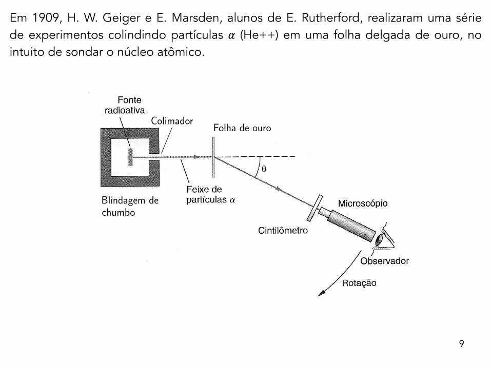
Em 1909, H. W. Geiger e E. Marsden, alunos de E. Rutherford, realizaram uma série de experimentos colindindo partículas 𝛼 (He++) em uma folha delgada de ouro, no intuito de sondar o núcleo atômico.

Aparato experimentalO modelo nuclear de Rutherford Espectros atomicos

Aula 5 4 / 17

Em 1909, H. W. Geiger e E. Marsden, alunos de E. Rutherford, realizaram umaserie de experimentos colindindo partıculas α (He++) em uma folha delgada deouro, no intuito de sondar o nucleo atomico. Abaixo encontra-se o diagramaesquematico do dispositivo experimental:

Blindagem dechumbo

ColimadorFolha de ouro

10

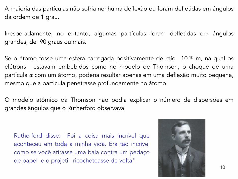
A maioria das partículas não sofria nenhuma deflexão ou foram defletidas em ângulos da ordem de 1 grau.

Inesperadamente, no entanto, algumas partículas foram defletidas em ângulos grandes, de 90 graus ou mais.

Se o átomo fosse uma esfera carregada positivamente de raio 10-10 m, na qual os elétrons estavam embebidos como no modelo de Thomson, o choque de uma partícula 𝛼 com um átomo, poderia resultar apenas em uma deflexão muito pequena, mesmo que a partícula penetrasse profundamente no átomo.

O modelo atômico da Thomson não podia explicar o número de dispersões em grandes ângulos que o Rutherford observava.

Rutherford disse: "Foi a coisa mais incrível que aconteceu em toda a minha vida. Era tão incrível como se você atirasse uma bala contra um pedaço de papel e o projetil ricocheteasse de volta".

11

Rutherford concluiu que as grandes deflexões obtidas experimentalmente poderiam resultar apenas de encontros das partículas 𝛼 com uma carga positiva confinada em um volume muito menor que o átomo como um todo.

Supondo que este "núcleo" fosse uma carga pontual, ele calculou a distribuição angular esperada para as partículas 𝛼 após a colisão.

Suas previsões sobre a variação da probabilidade de espalhamento em função do ângulo, da carga do núcleo e da energia cinética das partículas 𝛼 foram amplamente confirmadas em uma série de experimentos realizados em seu laboratório por Geiger e Marsden.

12

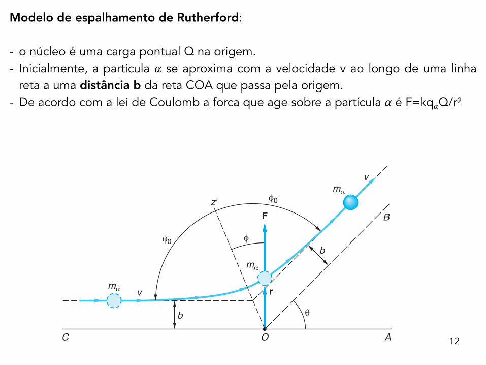
Modelo de espalhamento de Rutherford:

- o núcleo é uma carga pontual Q na origem. - Inicialmente, a partícula 𝛼 se aproxima com a velocidade v ao longo de uma linha

reta a uma distância b da reta COA que passa pela origem. - De acordo com a lei de Coulomb a forca que age sobre a partícula 𝛼 é F=kq𝛼Q/r2

4-2 Rutherford’s Nuclear Model 159

placed between it and the source. Most of the A particles were either undeflected or deflected through very small angles of the order of 1�. Quite unexpectedly, however, a few A particles were deflected through angles as large as 90� or more. If the atom con-sisted of a positively charged sphere of radius 10�10 m, containing electrons as in the Thomson model, only a very small deflection could result from a single encounter between an A particle and an atom, even if the A particle penetrated into the atom. Indeed, calculations showed that the Thomson atomic model could not possibly account for the number of large-angle scatterings that Rutherford saw. The unexpected scatterings at large angles were described by Rutherford with these words:

It was quite the most incredible event that ever happened to me in my life. It was as incredible as if you fired a 15-inch shell at a piece of tissue paper and it came back and hit you.

Rutherford’s Scattering Theory and the Nuclear AtomThe question is, then, Why would one obtain the large-angle scattering that Rutherford saw? The trouble with the Thomson atom is that it is too “soft”—the maximum force experienced by the A is too weak to give a large deflection. If the positive charge of the atom is concentrated in a more compact region, however, a much larger force will occur at near impacts. Rutherford concluded that the large-angle scattering obtained experimentally could result only from a single encounter of the A particle with a mas-sive charge confined to a volume much smaller than that of the whole atom. Assum-ing this “nucleus” to be a point charge, he calculated the expected angular distribution for the scattered A particles. His predictions of the dependence of scattering probabil-ity on angle, nuclear charge, and kinetic energy were completely verified in a series of experiments carried out in his laboratory by Geiger and Marsden.

We will not go through Rutherford’s derivation in detail but merely outline the assumptions and conclusions. Figure 4-5 shows the geometry of an A particle being scattered by a nucleus, which we take to be a point charge Q at the origin. Initially, the A particle approaches with speed v along a line a distance b from a parallel line

C O A

v

v

r

F

φ�

φ� φ

mα

mα

b

b

θ

mα

z�

B

FIGURE 4-5 Rutherford scattering geometry. The nucleus is assumed to be a point charge Q at the origin O. At any distance r the A particle experiences a repulsive force kqA Q�r 2. The A particle travels along a hyperbolic path that is initially parallel to line COA a distance b from it and finally parallel to line OB, which makes an angle U with OA. The scattering angle U can be related to the impact parameter b by classical mechanics.

TIPLER_04_153-192hr.indd 159 8/22/11 11:36 AM

13

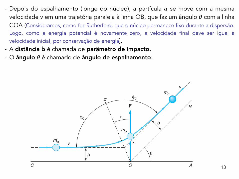
- Depois do espalhamento (longe do núcleo), a partícula 𝛼 se move com a mesma velocidade v em uma trajetória paralela à linha OB, que faz um ângulo 𝜃 com a linha COA (Consideramos, como fez Rutherford, que o núcleo permanece fixo durante a dispersão. Logo, como a energia potencial é novamente zero, a velocidade final deve ser igual à velocidade inicial, por conservação de energia).

- A distância b é chamada de parâmetro de impacto. - O ângulo 𝜃 é chamado de ângulo de espalhamento.

4-2 Rutherford’s Nuclear Model 159

placed between it and the source. Most of the A particles were either undeflected or deflected through very small angles of the order of 1�. Quite unexpectedly, however, a few A particles were deflected through angles as large as 90� or more. If the atom con-sisted of a positively charged sphere of radius 10�10 m, containing electrons as in the Thomson model, only a very small deflection could result from a single encounter between an A particle and an atom, even if the A particle penetrated into the atom. Indeed, calculations showed that the Thomson atomic model could not possibly account for the number of large-angle scatterings that Rutherford saw. The unexpected scatterings at large angles were described by Rutherford with these words:

It was quite the most incredible event that ever happened to me in my life. It was as incredible as if you fired a 15-inch shell at a piece of tissue paper and it came back and hit you.

Rutherford’s Scattering Theory and the Nuclear AtomThe question is, then, Why would one obtain the large-angle scattering that Rutherford saw? The trouble with the Thomson atom is that it is too “soft”—the maximum force experienced by the A is too weak to give a large deflection. If the positive charge of the atom is concentrated in a more compact region, however, a much larger force will occur at near impacts. Rutherford concluded that the large-angle scattering obtained experimentally could result only from a single encounter of the A particle with a mas-sive charge confined to a volume much smaller than that of the whole atom. Assum-ing this “nucleus” to be a point charge, he calculated the expected angular distribution for the scattered A particles. His predictions of the dependence of scattering probabil-ity on angle, nuclear charge, and kinetic energy were completely verified in a series of experiments carried out in his laboratory by Geiger and Marsden.

We will not go through Rutherford’s derivation in detail but merely outline the assumptions and conclusions. Figure 4-5 shows the geometry of an A particle being scattered by a nucleus, which we take to be a point charge Q at the origin. Initially, the A particle approaches with speed v along a line a distance b from a parallel line

C O A

v

v

r

F

φ�

φ� φ

mα

mα

b

b

θ

mα

z�

B

FIGURE 4-5 Rutherford scattering geometry. The nucleus is assumed to be a point charge Q at the origin O. At any distance r the A particle experiences a repulsive force kqA Q�r 2. The A particle travels along a hyperbolic path that is initially parallel to line COA a distance b from it and finally parallel to line OB, which makes an angle U with OA. The scattering angle U can be related to the impact parameter b by classical mechanics.

TIPLER_04_153-192hr.indd 159 8/22/11 11:36 AM

14

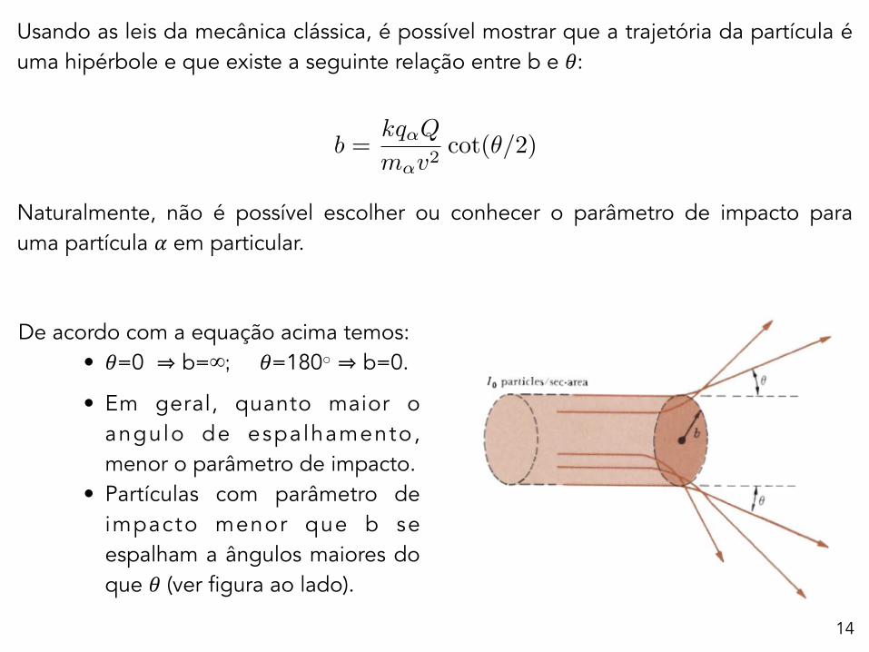
Usando as leis da mecânica clássica, é possível mostrar que a trajetória da partícula é uma hipérbole e que existe a seguinte relação entre b e 𝜃:

Naturalmente, não é possível escolher ou conhecer o parâmetro de impacto para uma partícula 𝛼 em particular.

F =1

4⇡"0

q↵QAu

r2

•b

b =1

4⇡✏0

q↵QAu

m↵v2cot

✓

2

q↵ ↵ QAu = ZAu r

↵ ✓

b ✓

• I0 ↵

I0 =num. partıculas

cm2 · seg

De acordo com a equação acima temos: • 𝜃=0 ⇒ b=∞; 𝜃=180○ ⇒ b=0.

• Em geral, quanto maior o angulo de espalhamento, menor o parâmetro de impacto.

• Partículas com parâmetro de impacto menor que b se espalham a ângulos maiores do que 𝜃 (ver figura ao lado).

b =kq↵Q

m↵v2cot(✓/2)

Seja I0 a intensidade do feixe de partículas incidentes por segundo e por unidade de área.

O número de partículas 𝛼 espalhadas por UM NÚCLEO por segundo cujo ângulo de espalhamento é maior que 𝜃 deve ser igual ao número de partículas 𝛼 espalhadas por um núcleo por segundo cujo parâmetro de impacto é menor que b(𝜃). Esse número é 𝜋b2I0.

A quantidade 𝜋b2, que tem dimensões de área, é chamada de seção de choque e é representada pela letra grega 𝜎. A seção de choque é definida como o número de partículas espalhadas por núcleo e por unidade de tempo dividido pela intensidade do feixe incidente.

O número TOTAL (i.e. por todos os núcleos) de partículas espalhadas por segundo é obtido multiplicando 𝜋b2I0 pelo número de núcleos da folha de metal.

15

F =1

4⇡"0

q↵QAu

r2

•b

b =1

4⇡✏0

q↵QAu

m↵v2cot

✓

2

q↵ ↵ QAu = ZAu r

↵ ✓

b ✓

• I0 ↵

I0 =num. partıculas

cm2 · seg

Seja n o número de núcleos por unidade de volume:

Seja A a área por onde passa o feixe e t a espessura da folha de metal.

O número total de núcleos na área coberta pelo feixe é: n × (A×t)

16

4-2 Rutherford’s Nuclear Model 161

number scattered per nucleus per unit time divided by the incident intensity. The total number of particles scattered per second is obtained by multiplying Pb2I0 by the number of nuclei in the scat-tering foil (this assumes the foil to be thin enough to make the chance of overlap negligible). Let n be the number of nuclei per unit volume:

n �R�g�cm3�NA�atoms�mol�

M�g�mol� �RNA

M atomscm3 4-4

For a foil of thickness t, the total number of nuclei “seen” by the beam is nAt, where A is the area of the beam (Figure 4-8). The total number scattered per second through angles greater than U is thus Pb2I0ntA. If we divide this by the number of A particles incident per second I0A, we get the fraction f scattered through angles greater than U:

f � Pb2 nt 4-5

EXAMPLE 4-2 Scattered Fraction f Calculate the fraction of an incident beam of A particles of kinetic energy 5 MeV that Geiger and Marsden expected to see for U � 90� from a gold foil (Z � 79) 10�6 m thick.

SOLUTION

1. The fraction f is related to the impact parameter b, the number density of nuclei n, and the thickness t by Equation 4-5:

f � Pb2nt

2. The particle density n is given by Equation 4-4:

n �RNA

M��19.3 g�cm3� �6.02 � 1023 atoms�mol�

197 gm�mol

� 5.90 � 1022 atoms�cm3 � 5.90 � 1028 atoms�m3

3. The impact param-eter b is related toU by Equation 4-3:

b �kqA QmA v2 cot

U

2��2� �79�ke2

2KA

cot 90�

2

��2� �79� �1.44 eV � nm��2� �5 � 106 eV� � 2.28 � 10�5 nm

� 2.28 � 10�14 m

4. Substituting these into Equation 4-5 yields f:

f � P�2.28 � 10�14 m�245.9 � 1028 atoms

m3 5 �10�6 m�� 9.6 � 10�5 � 10�4

Remarks: This outcome is in good agreement with Geiger and Marsden’s mea-surement of about 1 in 8000 in their first trial. Thus, the nuclear model is in good agreement with their results.

FIGURE 4-8 The total number of nuclei of foil atoms in the area covered by the beam is nAt, where n is the number of foil atoms per unit volume, A is the area of the beam, and t is the thickness of the foil.

Number of foil nucleiin beam is nAt

t

Area A of beam

TIPLER_04_153-192hr.indd 161 8/22/11 11:36 AM

✓

⇡b2I0

� = ⇡b2 ⌘ secao de choque

⇡b2I0

A

t

NAu = nAt

n

n =⇢Au

matomo

=⇢AuNA

Mmolar

• ✓

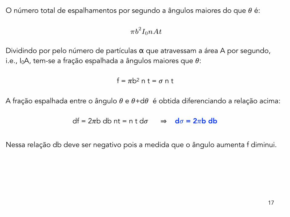
O número total de espalhamentos por segundo a ângulos maiores do que 𝜃 é:

Dividindo por pelo número de partículas α que atravessam a área A por segundo, i.e., I0A, tem-se a fração espalhada a ângulos maiores que 𝜃:

f = 𝜋b2 n t = 𝜎 n t

A fração espalhada entre o ângulo 𝜃 e 𝜃+d𝜃 é obtida diferenciando a relação acima:

df = 2𝜋b db nt = n t d𝜎 ⇒ d𝜎 = 2𝜋b db

Nessa relação db deve ser negativo pois a medida que o ângulo aumenta f diminui.

17

⇡b2I0nAt

↵ A

I0A ✓

f = ⇡b2nt

✓ ✓ + d✓

df = 2⇡b db nt = n t d�

db f

d�

d⌦

I0d�

d⌦d⌦ = Numero de espalhamentos entre angulo solido

⌦ e ⌦ + d⌦ por unidade de tempo

d⌦ = 2⇡ sin✓d✓

I0d�

d⌦d⌦ = 2⇡I0b | db |

b ✓

db = �1

8⇡✏0

q↵QAu

m↵v2

1

sin2✓2

d✓

A seção de choque diferencial dσ/d𝛺 é definida como

18

⇡b2I0nAt

↵ A

I0A ✓

f = ⇡b2nt

✓ ✓ + d✓

df = 2⇡b db nt = n t d�

db f

d�

d⌦

I0d�

d⌦d⌦ = Numero de espalhamentos entre angulo solido

⌦ e ⌦ + d⌦ por unidade de tempo

d⌦ = 2⇡ sin✓d✓

I0d�

d⌦d⌦ = 2⇡I0b | db |

b ✓

db = �1

8⇡✏0

q↵QAu

m↵v2

1

sin2✓2

d✓

Número de espalhamentos por unidade de tempo entre o ângulo sólido Ω e Ω + dΩ

O número de partículas espalhadas deve ser tal que

onde usamos d𝜎 = 2𝜋b db (ver slide anterior). O módulo foi tomado para que se integre do ângulo mínimo até o ângulo máximo. Repare que ao se diminuir b o ângulo 𝜃 cresce.

Agora, diferenciando a expressão para b obtida antes (slide 14) obtemos:

I0d�

d⌦d⌦ = I0d� = I0(2⇡b|db|)

b =kq↵Q

m↵v2cot(✓/2) ) db =

kq↵Q

m↵v2(�1/2)

sin2(✓/2)d✓

Eq. (*)

Substituindo as expressões para b e db na Eq (*) e usando d𝛺=2𝜋sin𝜃d𝜃, obtemos:

que é a seção de choque diferencial de espalhamento de Rutherford.

Agora, lembremos que a fração de partículas espalhada em ângulos maiores que 𝜃 é f = 𝜎 n t (veja slide 17); logo:

19

d�

d⌦=

✓kq↵Q

2m↵v2

◆2 1

sin4(✓/2)

df

d⌦= nt

d�

d⌦=

✓kq↵Q

2m↵v2

◆2 nt

sin4(✓/2)

20

d� = 2⇡b | db |

4⇡

✓1

8⇡✏0

q↵QAu

m↵v2

◆2cot

✓

2

sin2✓2

d✓

= 2⇡

✓1

8⇡✏0

q↵QAu

m↵v2

◆2 1

sin4✓2

sin✓d✓

=

✓1

8⇡✏0

q↵QAu

m↵v2

◆2 1

sin4✓2

d⌦

=d�

d⌦d⌦

✓cos

✓

2 = 12sin✓

sin✓2

◆d⌦ = 2⇡sin✓d✓

d�

d⌦=

✓1

8⇡✏0

q↵QAu

m↵v2

◆2 1

sin4✓2

I

↵

O número de partículas espalhadas entre 𝜃 e 𝜃+d𝜃 por segundo é obtido multiplicando pela área A do feixe e pelo número de partículas incidentes por unidade de área e tempo, I0:

Essas partículas atravessam a região anular maior na figura por unidade de tempo.

N = I0Adf

d⌦=

✓kq↵Q

2m↵v2

◆2 I0Ant

sin4(✓/2)

NArea

=1

Area

1

4⇡✏0

Z e2

m↵v2

!2I0NAu

sin4✓2

•

• sin�4✓

2Z

2v2

•

Geiger e Marsden confirmaram todas as previsões da expressão acima: a dependência com o ângulo 𝜃, com a carga elétrica, com a velocidade e com a espessura do alvo.

Isso mostrou que o modelo atômico nuclear era a base correta para o estudo dos fenômenos atômicos e nucleares.

21

Se dividirmos pela área da região anular maior temos o número de partículas espalhadas entre 𝜃 e 𝜃+d𝜃 por segundo por unidade de área.

Isso é o que um detetor colocado em um ângulo 𝜃 pode medir.

NArea

=1

Area

✓kq↵Q

2m↵v2

◆2 I0Ant

sin4(✓/2)

22

No entanto, o modelo de Rutherford é previsto ser instável pela física clássica!

A emissão de radiação contínua impede a estabilidade de um sistema clássico assim!

NArea

=1

Area

1

4⇡✏0

Z e2

m↵v2

!2I0NAu

sin4✓2

•

• sin�4✓

2Z

2v2

•