BRIDGING THE ENERGY DIVIDE AND SECURING HIGHER … · Gabriela, Gabriela L., Kristen, Monika, and Rina for all the support and encouragement received throughout the development of

BRIDGING THE ENERGY DIVIDE AND SECURING HIGHER COLLECTIVE

WELLBEING IN A CLIMATE-CONSTRAINED WORLD

Aline Ribas

Tese de Doutorado apresentada ao Programa de

Pós-graduação em Planejamento Energético,

COPPE, da Universidade Federal do Rio de

Janeiro, como parte dos requisitos necessários à

obtenção do título de Doutor em Planejamento

Energético.

Orientadores: Roberto Schaeffer

André Frossard Pereira de Lucena

Rio de Janeiro

Abril de 2017



Aline Ribas

TESE SUBMETIDA AO CORPO DOCENTE DO INSTITUTO ALBERTO LUIZ

COIMBRA DE PÓS-GRADUAÇÃO E PESQUISA DE ENGENHARIA (COPPE) DA

UNIVERSIDADE FEDERAL DO RIO DE JANEIRO COMO PARTE DOS

REQUISITOS NECESSÁRIOS PARA A OBTENÇÃO DO GRAU DE DOUTOR EM

CIÊNCIAS EM PLANEJAMENTO ENERGÉTICO.

Examinada por:

RIO DE JANEIRO, RJ - BRASIL

ABRIL DE 2017

Prof. Maurício Tiomno Tolmasquim, D.Sc.

Prof. Angelo Costa Gurgel, D.Sc.

Prof. Suzana Khan Ribeiro, D.Sc.

Prof. Alexandre Salem Szklo, D.Sc.

Prof. Roberto Schaeffer, Ph.D.

iii

Ribas, Aline

Bridging the energy divide and securing higher

collective wellbeing in a climate-constrained world /

Aline Ribas - Rio de Janeiro: UFRJ/COPPE, 2017.

XIX, 210 p.: il.; 29,7 cm.



Tese (doutorado) − UFRJ / COPPE / Programa de

Planejamento Energético, 2017.

Referências Bibliográficas: p. 143-176.

1. Energy consumption 2. Human wellbeing 3. Carbon

budgets 4. Emissions shortfalls 5. Mitigation strategies I.

Schaeffer, Roberto et al. II. Universidade Federal do Rio

de Janeiro, COPPE, Programa de Planejamento

Energético. III. Título.

iv

“Happiness is the meaning and the purpose of life,

the whole aim and end of human existence.”

Aristotle (ca. 350 B.C.)

“All things share the same breath - the beast, the tree, the man. The air shares its

spirit with all the life it supports.”

Chief Seattle (1854)

"Procuremos más ser padres de nuestro porvenir que hijos de nuestro

pasado."

Miguel de Unamuno (1864-1936)

“The earth offers enough for everyone’s need, not for everyone’s greed”

Mahatma Gandhi (1869-1948)

“Somos responsáveis por aquilo que fazemos, o que não fazemos e o que

impedimos de fazer.”

Albert Camus (1913-1960)

“I call the transformed world toward which we can move ‘sustainable,’ by which I

mean (...) a world that evolves, as life on earth has evolved for three billion

years, toward ever greater diversity, elegance, beauty, self-awareness,

interrelationship, and spiritual realization.”

Donatella H. Meadows (1941-2001)

v

To every human being that has yet to gain access to reliable, sustainable and modern

energy, and/or attain swasthya (true wellbeing).

vi

AGRADECIMENTOS

Primeiramente, agradeço por mais uma valiosa oportunidade de desfrutar do

ambiente multidisciplinar tão enriquecedor que o Programa de Planejamento Energético

da COPPE oferece. Sou grata ainda ao International Institute for Sustainable

Development (IISD), à Fundação Brasileira para o Desenvolvimento Sustentável

(FBDS), e ao Stockholm Environment Institute (SEI) pelas participações em trabalhos

que me permitiram aprofundar minha pesquisa nas questões sociais e ambientais

relevantes ao planejamento energético. Dedico um agradecimento especial ao Roberto

Paulo Cezar de Andrade pelo material que, juntamente com trabalhos do Professor José

Goldemberg em pobreza energética, serviu de inspiração inicial para esta tese.

Aos meus orientadores, Professores Roberto Schaeffer e André Lucena, agradeço

pelo acompanhamento, pela paciência e pela orientação recebida ao longo dos últimos

anos e pelas várias oportunidades de aprendizado. Agradeço também ao Professor

Alexandre Szklo não só pela participação na banca examinadora, mas por todas as

contribuições tanto para o amadurecimento quanto para a finalização desta tese. Ao

Professor Maurício Tolmasquim por aceitar participar da banca na última hora. Aos

Professores Suzana Kahn Ribeiro e Angelo Costa Gurgel, também gostaria de deixar

registrado um agradecimento especial pela avaliação e debate enriquecedor.

Agradeço também ao apoio constante de toda equipe administrativa do PPE, em

especial à Sandra Bernardo, ao Paulo Feijó e ao Fernando Moreno. Obrigada aos

colegas do PPE, sobretudo a Ana Carsalade e Luis Saporta pelo convívio enriquecedor.

Ao CNPq agradeço pelo apoio financeiro durante os primeiros anos do doutorado.

Agradeço à minha família pelo apoio incondicional, principalmente nos

momentos mais intensos dessa jornada de aprendizado e dedicação: meu marido Felipe

e meus filhos Arthur e Gustavo. E à minha mãe Jane e ao meu pai Arthur, já falecido,

dedico o meu mais profundo e carinhoso agradecimento por nunca terem medido

esforços para me presentear com o que há de mais precioso para o enriquecimento

humano: o conhecimento.

Finally, I would like to acknowledge and extend my heartfelt gratitude to my very

dear friends Adriana, Alejandro, Andrea, Astrid, Claudia, Cristi, Cristina, Daniela,

Gabriela, Gabriela L., Kristen, Monika, and Rina for all the support and encouragement

received throughout the development of this thesis. And above all, I am deeply thankful

to the constant guidance and support of the teachings and practice of Yoga.

vii

Resumo da Tese apresentada à COPPE/UFRJ como parte dos requisitos necessários

para a obtenção do grau de Doutor em Ciências (D.Sc.)

VENCENDO A INIQUIDADE ENERGÉTICA E ASSEGURANDO O AUMENTO

DO BEM-ESTAR COLETIVO EM UM MUNDO COM LIMITAÇÕES IMPOSTAS

PELO CLIMA

Aline Ribas

Abril/2017



Programa: Planejamento Energético

Não obstante os ganhos expressivos na quantidade de energia disponível obtidos

ao longo dos últimos dois séculos, seus benefícios continuam a ser distribuídos de

forma extremamente desigual. O vencimento dessa iniquidade contribui para aumentar

ainda mais o desafio de se atingir a estabilização do clima. Essa tese se propõe a

examinar uma eventual incompatibilidade entre esses dois objetivos. Para tanto, estima-

se a quantidade de energia que seria necessária para assegurar o aumento do bem-estar

global até meados do século a partir de regressões log-log e calcula-se as emissões de

carbono correspondentes com base nas intensidades de emissões de diferentes cenários

do modelo de avaliação integrada MESSAGE. Utiliza-se uma proxy de bem-estar

humano selecionada entre indicadores alternativos ao PIB, abrangendo os três pilares do

desenvolvimento sustentável.

Os resultados indicam que mesmo com a adoção de novas políticas e ações de

mitigação, emissões associadas ao aumento do bem-estar em todas as regiões onde

melhorias ainda são necessárias, as quais representam 78 por cento da população global,

poderiam exceder em até uma vez e meia as quotas consistentes com a meta de

estabilização abaixo de 2 oC e, ainda mais, no caso de metas mais rigorosas. Conclui-se

que mudanças nas escolhas de estilo de vida nos países desenvolvidos, como transporte

pessoal e dieta, poderão ser essenciais para permitir o incremento de emissões

necessário para se assegurar o aumento de bem-estar coletivo no resto do mundo.

viii

Abstract of Thesis presented to COPPE/UFRJ as a partial fulfillment of the

requirements for the degree of Doctor of Science (D.Sc.)



Aline Ribas

April/2017

Advisors: Roberto Schaeffer


Department: Energy Planning

In spite of the impressive gains in available energy over the last two centuries, the

associated benefits remain unevenly distributed. Bridging this divide only adds to the

already daunting challenge of securing climate stabilization. This thesis examines the

potential incompatibility between these two efforts by estimating the additional energy

needed to secure higher collective wellbeing across the globe by mid-century based on

regional energy elasticities of wellbeing derived from regressions using linear log-log

models and by calculating the associated carbon emissions based on emission intensities

obtained from different climate action scenarios of the integrated assessment model

MESSAGE. A proxy measure for human wellbeing is selected from existing alternative

aggregate indicators to GDP, encompassing all three pillars of sustainable development.

Results indicate that even with new climate policies and actions, emissions

associated with higher wellbeing in all regions where improvements are still needed,

which represent 78 percent of the global population, could still reach up to one and a

half times estimated 2 degrees Celsius budgets, and even more so for lower temperature

increase targets. Given the scale of the overall gaps, effective changes in lifestyle

choices in advanced countries, such as those associated with home energy use, private

travel, and diet, would be needed to make room for the additional emissions needed to

secure higher collective wellbeing in the rest of the world.

ix

Contents 1. Introduction ............................................................................................................... 1

2. Energy use and human development: an overview ................................................... 7

2.1. Energy transitions: from hunter-gatherers to the first high-energy civilization . 7

2.2. The energy divide: minimum thresholds and access to modern energy services

11

2.3. Energy use in a climate-constrained world ...................................................... 17

2.3.1. The climate stabilization challenge ............................................................ 18

2.3.2. Carbon budgets and emissions pathways associated with the “2 oC target”

26

2.3.3. Carbon impact of energy use ...................................................................... 30

2.4. The energy use-human development nexus: a literature overview .................. 32

2.4.1. Traditional focus on economic growth ...................................................... 32

2.4.2. Recent interest in broader aspects of human development ........................ 36

3. Human wellbeing: concepts and measurements from a development perspective . 44

3.1. Early conceptualizations: from material individualism to spiritual collectivism

45

3.1.1. Hedonism: wellbeing as maximization of individual pleasure .................. 46

3.1.2. Eudaimonism: wellbeing as the actualization of human potentials ........... 47

3.1.3. Eastern conceptualizations: wellbeing through self-transcendence ........... 48

3.2. Modern conceptualizations: from economic growth to sustainability ............. 51

3.2.1. The predominant one-dimensional conceptualization centered on economic

growth 52

3.2.2. Multi-dimensional conceptualizations: seeking a coherent theory of

wellbeing ................................................................................................................ 54

3.3. Traditional measurements: GNP, GDP, GNI ................................................... 58

3.3.1. A brief history of national income and product statistics .......................... 60

3.3.2. Shortcomings of GDP as a measure of societal wellbeing ........................ 64

3.4. New measurements: alternative indicators to GDP .......................................... 70

3.4.1. Aggregate indicators using the replacing GDP approach: HDI, HSDI, and

HPI 74

3.4.2. Aggregate indicators using the adjusting GDP approach: GPI, IEWB, SSI,

and IWI ................................................................................................................... 76

x

3.4.3. Aggregate indicators using the supplementing GDP approach: SPI .......... 81

3.4.4. Barriers to the deployment of new measurements ..................................... 82

4. Bridging the energy divide: a quantitative assessment ........................................... 90

4.1. Selecting proxies for human wellbeing from alternative indicators to GDP .... 92

4.2. Data preparation and analysis ........................................................................... 94

4.2.1. Data collection ........................................................................................... 94

4.2.2. Regional aggregation ................................................................................. 95

4.2.3. Dataset analysis .......................................................................................... 96

4.3. Projecting aggregate levels of human wellbeing into 2050 .............................. 98

4.4. Correlating human wellbeing and energy consumption ................................. 101

4.5. Estimating the additional energy needed and associated carbon emissions ... 106

5. Results ................................................................................................................... 109

5.1. Additional energy needed and associated emissions ...................................... 109

5.1.1. In ASIA .................................................................................................... 110

5.1.2. In the Middle East and Africa (MAF) ...................................................... 111

5.1.3. In Latin America (LAM) .......................................................................... 112

5.1.4. In Economies in Transition (EIT) ............................................................ 112

5.2. Wellbeing versus climate stabilization: comparing emissions pathways ....... 113

5.2.1. Associated emissions under no-action scenario ....................................... 113

5.2.2. Climate action scenarios .......................................................................... 118

5.2.3. Associated emissions under Action as of 2020-500 scenario .................. 118

5.2.4. Associated emissions under Action as of 2020-450 scenario .................. 121

5.2.5. Associated emissions under Delayed action-500 scenario ....................... 123

5.3. Wellbeing versus climate stabilization: assessing the gaps ............................ 125

6. Analysis of results and recommendations ............................................................. 128

6.1. Answering question number 1: how much energy consumption, and its

corresponding CO2 emissions, would be needed to bridge the energy divide and

enable the achievement of higher levels of collective wellbeing? ........................... 129

6.2. Answering question number 2: Would the existing carbon budgets be affected?

129

6.3. Answering question number 3: If so, what part(s) of the world would be mostly

at risk? ...................................................................................................................... 130

6.4. Answering question number 4: what needs to be done to bridge the energy

xi

divide and increase wellbeing while staying within existing carbon budgets? ........ 130

6.5. Recommendations .......................................................................................... 132

7. Final remarks ......................................................................................................... 137

7.1. Contributions and policy implications ............................................................ 137

7.2. Suggestions for future research ...................................................................... 140

References .................................................................................................................... 143

Appendix A – Table of selected studies on energy consumption, GDP growth, and CO2

emissions ...................................................................................................................... 177

Appendix B – Table of key alternative indicators to GDP. .......................................... 181

Appendix C – Table of key data and calculations. ....................................................... 182

Appendix D – Table of region categorization. ............................................................. 185

Appendix E – Comparison with previous quantification efforts. ................................. 187

Appendix F – Assessing the gaps in all regions (including OECD90). ....................... 190

xii

List of Figures Figure 1 - Timeline of energy eras and great transitions. ................................................. 8

Figure 2 - Selected dimensions of human development (standard of living, knowledge,

and longevity) and annual per capita energy consumption rate, 1870–2005. ........ 12

Figure 3 - Selected dimensions of human development (standard of living, knowledge,

and longevity) and annual per capita energy consumption rate: Absolute gaps

between OECD countries and the rest of the world, 1870-2005. ........................... 14

Figure 4 - Global energy divide in annual per capita primary energy consumption rates.

................................................................................................................................ 15

Figure 5 - Primary energy consumption levels in the developing world. ...................... 16

Figure 6 - Radiative forcing of climate between 1750 and 2011 (in W/m2). Solid lines

provide the range of uncertainty (5 to 95 percent confidence). .............................. 20

Figure 7 - Atmospheric carbon dioxide concentrations (in ppm) and global temperature

anomalies (in oC) over the years 1880 to 2015. ...................................................... 22

Figure 8 - Simulated global mean surface temperature increase as a function of

cumulative total global CO2 emissions and cumulative emissions budget associated

with the 2 oC target. ................................................................................................ 27

Figure 9 - Saturation and decoupling trend between HDI and carbon emissions (upper

plot, 115 countries) and between HDI and energy consumption (114 countries for

1990 data and 116 countries for 2000 data and 2010 data) from 1990 to 2010. .... 39

Figure 10 - Income (in per capita GDP) versus wellbeing. ............................................ 68

Figure 11 - Timeline of Key Alternative Indicators to GDP. ......................................... 73

Figure 12 - Selection process for the appropriate proxy(ies) for human wellbeing. ...... 92

Figure 13 - Observed changes in energy consumption measured in per capita primary

energy consumption (pcEC), in wellbeing measured in per capita IWI (pcIWI), in

income measured in per capita GDP (pcGDP) and in HDI for the overall sample

between 1990 and 2010. ......................................................................................... 97

Figure 14 - Observed trends and projections (faded lines) of human wellbeing measured

in per capita IWI (pcIWI) contrasted with observed trends and projections (faded

lines) of per capita GDP (pcGDP). ....................................................................... 100

Figure 15 - Correlation between human wellbeing measured in per capita IWI and

energy consumption measured in per capita primary energy over the one hundred

and eighteen countries covered here for the year 2000 (shown in log-log space).102

xiii

Figure 16 - Correlations of human wellbeing measured in per capita IWI (pcIWI) and

energy consumption measured in per capita energy consumption (pcEC) in log-log

form across four of the RC5 regions in the year 2010.......................................... 104

Figure 17 - Change in elasticity (b values) over time................................................... 105

Figure 18 - Estimated annual primary energy and CO2 emissions pathways for

achieving higher levels of human wellbeing in ASIA, EIT, LAM, and MAF,

compared to two stabilization scenarios from the IAM MESSAGE (Immediate

action-450 and Immediate action-500), which would yield reasonably high and

even chances of achieving 2oC, respectively. ....................................................... 115

Figure 19 - Estimated cumulative primary energy and CO2 emissions for achieving

higher levels of human wellbeing in ASIA, EIT, LAM, and MAF in 2011-2030

and 2011-2050, compared to two standard benchmark policy scenarios from the

IAM MESSAGE v.4 (Immediate action-450 and Immediate action-500), which are

associated with reasonably high and even chances of meeting the 2 oC target,

respectively. .......................................................................................................... 116

Figure 20 - Estimated annual primary energy and CO2 emissions for achieving higher

levels of human wellbeing in ASIA, EIT, LAM, and MAF in the Action as of

2020-500, compared to projections based on two stabilization scenarios from the

IAM MESSAGE (Immediate action-450 and Immediate action-500), which would

yield reasonably high and even chances of achieving 2oC, respectively.............. 120


levels of human wellbeing in ASIA, EIT, LAM, and MAF in the Action as of

2020-450, compared to projections based on two stabilization scenarios from the




levels of human wellbeing in ASIA, EIT, LAM, and MAF in the Delayed action-

500 scenario, compared to projections based on the stabilization scenarios from the



xiv

List of Tables Table 1 - Selected non-market valuation methods applied to ecosystem services. ........ 86

Table 2 - Key data values by year and region. ............................................................... 96

Table 3 - Per capita IWI across all RC5 regions in 2010 and projected to 2030 and 2050.

................................................................................................................................ 99

Table 4 - Regression results from Equation [1]. ........................................................... 103

Table 5 - Compound annual rates of change (%) in elasticity...................................... 106

Table 6 - Compound annual rates of change (%) in CO2 emission intensity. .............. 108

Table 7 - Annual results from Equations [3] and [4]. ................................................... 109

Table 8 - Cumulative results from Equations [3] and [4]. ............................................ 110

Table 9 - Emissions scenarios. ..................................................................................... 118

Table 10 - Compound annual rates of change (%) in CO2 emission intensity on the

Action as of 2020-500. ......................................................................................... 119


Action as of 2020-450. ......................................................................................... 121


Delayed action-500 scenario. ............................................................................... 123

Table 13 – Wellbeing emissions shortfall by 2050 per emissions scenario compared to

the 450-ppm budget. ............................................................................................. 126

Table 14 – Wellbeing emissions shortfall by 2050 per emissions scenario compared to

the 500-ppm budget. ............................................................................................. 126

List of Tables in Appendices

Table A 1 - Selected studies on energy consumption, GDP growth, and CO2 emissions.

.............................................................................................................................. 177

Table B 1 - Key alternative indicators to GDP. ............................................................ 181

Table C 1 – Description of key data and calculations. ................................................. 182

Table D 1 - Region categorization. ............................................................................... 185

xv

Table F 1 - Emissions shortfall by 2050 per emissions scenario compared to the 450-

ppm budget. .......................................................................................................... 190

Table F 2 - Emissions shortfall by 2050 per emissions scenario compared to the 500-

ppm budget. .......................................................................................................... 191

xvi

List of Acronyms

ANS − Adjusted Net Savings

AR − Assessment Report

BCE − Before Common Era

BECCS − Bioenergy with carbon capture and storage

BP − British Petroleum

BRICS − Brazil, Russia, India, China and South Africa

CBA − Cost-Benefit Analysis

CCS − Carbon Capture and Storage

CDR − Carbon Dioxide Removal

CE − Common Era

CEC − Commission of the European Communities

CH4 − Methane

CMEPSP − Commission on the Measurement of Economic Performance and Social

Progress

CO2 − Carbon Dioxide

CO2eq − Carbon Dioxide Equivalent

COP − Conference of the Parties

CSLS − Centre for the Study of Living Standards

CSP − Concentrated Solar Power

DAC − Direct Air Capture

EBPT − European Biofuels Technology Platform

EC − Energy Consumption

EEA − European Environment Agency

EIT − Economies in Transition

EJ − Exajoule

FCCC − Framework Convention on Climate Change

GDP − Gross Domestic Product

GHG − Greenhouse Gases

GJ − Gigajoule

GNH − Gross National Happiness

GNI − Gross National Income

xvii

GNP − Gross National Product

Gt – Gigaton

GPI − Genuine Progress Indicator

HDI − Human Development Index

HLY − Happy Life Years

HPI − Happy Planet Index

HSDI − Human Sustainable Development Index

IAM − Integrated Assessment Model

IAMC − Integrated Assessment Modeling Consortium

IEA − International Energy Agency

IEAGHG − IEA Greenhouse Gas R&D Programme

IEG − International Evaluation Group

IEWB − Index of Economic Wellbeing

IHDP − International Human Dimensions Programme

IIASA − International Institute for Applied Systems Analysis

IMF − International Monetary Fund

INDC − Intended Nationally Determined Contribution

IPCC − Intergovernmental Panel on Climate Change

IRENA − International Renewable Energy Agency

ISEW − Index of Sustainable Economic Welfare

IWI − Inclusive Wealth Index

koe − Kilogram oil equivalent

kV − Kilovolts

kW − Kilowatt

kWh − Kilowatt-hour

LAM − Latin America

LIMITS − The Low climate Impact scenarios and the Implications of required Tight

emission control Strategies

MAF − Middle East and Africa

MEA − Millennium Ecossystem Assessment

MESSAGE − Model for Energy Supply Systems And their General Environmental

impact

MEW − Measure of Economic Welfare

MW − Megawatt

xviii

N2O − Nitrous Oxide

NEF − New Economics Foundation

NOAA − National Oceanic and Atmospheric Administration

OECD − Organisation for Economic Co-operation and Development

ppm − parts per million

PPP − Purchase Power Parity

PV − Photovoltaics

RC − Region Categorization

RCP − Representative Concentration Pathways

RF − Radiative Forcing

SD − Sustainable Development

SEDA − Sustainable Economic Development Assessment

SNA − System of National Accounts

SPI − Social Progress Index

SSF − Sustainable Society Foundation

SSI − Sustainable Society Index

TAB − Threshold Avoidance Budget

TEB − Threshold Exceedance Budget

UN − United Nations

UNDP − UN Development Programme

UNEP − UN Environmental Programme

UNESCAP − UN Economic and Social Commission for Asia and the Pacific

UNESCO − United Nations Educational, Scientific and Cultural Organization

UNFCCC − UN Framework Convention on Climate Change

UNGA − UN General Assembly

UNU − University of the United Nations

USD − United States Dollar

W/m2 − Watt per square meter

WCED − World Commission on Environment and Development

WEO − World Energy Outlook

WG − IPCC Working Group

WHO − World Health Organization

WMO − World Meteorological Organization

WTA − Willingness to Accept

xix

WTP − Willingness to Pay

WVS − World Values Survey

ZEP − Zero Emission Fossil Fuel Power Plants

1

1. Introduction

Energy has played a vital role in humanity’s struggle for subsistence as an

essential input for food production, heat generation, and access to modern energy

services. It also became a key component in several aspects of human development and

wellbeing, such as educational opportunities, general health improvement, and food

security (MARTINEZ AND EBENBACK, 2008). It has been deemed indispensable for

eradicating poverty and inequality and achieving sustainable development (WCED,

1987; UNGA, 2015), a concept that postulates the existence of inextricable linkages

among economic, social and environmental factors.

The origins of the link between energy use and human development can be traced

straight back to the domestication of fire, the first extrasomatic energy conversion

mastered by humans (SMIL, 2004), dated to some 500,000 years ago (JAMES et al.,

1989; CARBONNIER AND GRINEVALD, 2012). However, significant use of energy

resources followed by technological progress leading to meaningful economic

expansion did not start until around two centuries ago in a few European countries

(SMIL, 2004), and continues to unfold in several developing countries.

Undoubtedly, the prosperity brought forth by the so-called thermo-industrial

revolution has led, directly and indirectly, to remarkable improvements in the wellbeing

of populations, notably healthier and longer lifespans, greater access to knowledge and

formal education, and improved standards of living. Energy use has fostered economic

growth, which, in turn, triggered demand for more and better-quality energy services.

As such, energy use has gradually moved from low quality fuels to high quality fuels,

from wood to coal, coal to petroleum, and petroleum to electricity.

The amount of energy consumed per capita in a society is said to be a good

measure of its relative state of advance (WHITE, 1959 and ODUM, 1971). In average,

the gross annual energy consumption per capita increased from about 10 gigajoules (GJ)

at the time of the Roman Empire to about 15 GJ in 1700 (SMIL, 2008, 2010a, and

2011). By 1800, it had reached about 50 GJ in the United Kingdom alone, presumably

the world’s highest per capita energy consumption at the time (WARDE, 2007; cited in

2

SMIL, 2011). Then by 2010, it reached 135 GJ in the United Kingdom and an

astounding 300 GJ in the United States.1 Compared to 1900, the global average per

capita energy consumption rate increased over fivefold, having reached 79 GJ by 2010.2

It is noteworthy that these improvements are far more impressive when expressed in

terms of actually available useful energy instead of gross primary energy inputs, in view

of technical advances that have improved typical efficiencies of all principal

commercial energy conversions over the last century (SMIL, 2000, 2010a, and 2011).

According to SMIL (2000), the world had at its disposal at least twenty-five times more

useful commercial energy in the year 2000 than in 1900.

In spite of the impressive gains in available energy over the last two centuries, the

associated benefits remain unevenly distributed and a significant share of the world’s

population still dwells in energy poverty. By 2010, around 3 billion people, almost half

of the world population, had an annual per capita primary energy consumption equal to

or below 50 GJ, a rate that has been associated with a minimum quality of life (SMIL,

2010a), and still lacked access to basic modern energy services. In fact, more than one

third of the world population enjoyed an average primary energy consumption rate

equal to or even below 30 GJ, which is roughly one seventh the average energy use in

affluent countries.3 Moreover, almost 1 billion people are expected to be added to the

population in the least developed part of the world by 2050 (UN, 2015), where annual

primary energy consumption rates fall below 15 GJ per capita, on average.4

Meanwhile, the burning of increased quantities of coal and petroleum-based fuels

has been the major cause of human induced climate change and is, therefore, considered

the main contributing factor to the upward trend in Earth’s surface temperature since

1950 (IPCC, 2014a). Annual carbon dioxide (CO2) emissions from fossil fuel

combustion for energy production and use have increased over 100 percent since 1970,

in spite of the significant reductions in the CO2 intensity of energy consumption seen in

1 Based on 2010 energy use data from the World Development Indicators (WORLD BANK, 2016) in kilograms of oil equivalent (koe) per capita converted to billion Joules (GJ) using IEA’s energy unit converter (OECD/IEA, 2016a). 2 Based on 2010 energy use data from the World Development Indicators (WORLD BANK, 2016) and IEA’s energy unit converter (OECD/IEA, 2016a). 3 Based on a calculated average of 201 GJ/capita for OECD countries using 2010 energy use data from the World Development Indicators (WORLD BANK, 2016). 4 Based on 2010 energy use data from the World Development Indicators (WORLD BANK, 2016).

3

the same period (BLANCO et al., 2014). They are expected to continue increasing in

the near future, as fossil fuels are likely to remain the dominant sources of energy

(CLARKE et al., 2014; OECD/IEA, 2015b).

Hence, it is clear that higher levels of energy consumption will be needed to

bridge the energy divide and enable the achievement of higher levels of human

wellbeing across the globe. However, at current decarbonisation rates and state of

knowledge and technology, the corresponding CO2 emissions associated with such

additional energy levels could compromise internationally agreed efforts towards

climate stabilization. In 2010, the Parties to the Climate Change Convention agreed that,

in order to achieve the necessary climate stabilization, global average temperature

increase should be limited to “below 2 degrees Celsius” (oC) above pre-industrial levels

(UNFCCC, 2010), the so-called “2 oC target”.5

By December 2015, one hundred and eighty seven countries that accounted for

over 96 percent of global CO2 equivalent emissions in 2012 had submitted climate

pledges (so-called “Intended Nationally Determined Contributions” [INDCs]) outlining

carbon reduction targets based on post-2020 action (KNUTTI et al., 2016; ROGELJ et

al., 2016a). However, according to recent studies (UNEP, 2015; ROGELJ et al., 2016a),

in the absence of additional emission reduction efforts, the estimated carbon budgets

associated with the 2 oC target could be consumed as soon as 2030, and emissions

would equate to scenarios that limit global average temperature increase in excess of the

intended 2 oC target (e.g. median of 3.2 oC by 2100 at a 66 percent chance) (ROGELJ et

al., 2016a). In this context, the additional energy needed to achieve higher levels of

collective wellbeing only adds to the already daunting challenge of securing climate

stabilization.

In light of these considerations, answers to the following pressing questions

should be sought:

5 This target was recently revised to “well below 2 oC” in the 2015 Paris Conference (UNFCCC, 2015).

4

1. How much energy consumption, and its corresponding CO2 emissions,

would be needed to bridge the energy divide and enable the achievement of

higher levels of collective wellbeing?

2. Would existing carbon budgets associated with climate stabilization be

affected?

3. If so, what part(s) of the world would be mostly at risk? And

4. What needs to be done to bridge the energy divide and increase wellbeing

while staying within existing carbon budgets?

In spite of the extensive literature on the relationship between energy

consumption and economic growth, measured in terms of Gross Domestic Product

(GDP) (CHEN et al., 2012; OZTURK, 2010), including a number of studies

encompassing CO2 emissions (OMRI, 2013), only a small number of studies has

examined the relationship between energy consumption and human development

beyond its economic dimension (PASTERNAK, 2000; SMIL, 2003, DIAS et al., 2006;

MARTINEZ AND EBENHACK, 2008; JACKSON, 2009; STEINBERGER AND

ROBERTS, 2009 and 2010; SMIL, 2010a; COSTA et al., 2011; MAZUR, 2011;

PASTEN AND SANTAMARINA, 2012; RAO AND BAER, 2012; STEINBERGER et

al., 2012; STECKEL et al., 2013; JORGENSON, 2014; UGURSAL, 2014; and LAMB

AND RAO, 2015).

To the author’s knowledge, only four studies have actually attempted to quantify

the energy needed to achieve certain levels of human wellbeing, namely PASTERNAK

(2000), COSTA et al. (2011), UGURSAL (2014), and LAMB AND RAO (2015). Of

those, only COSTA et al. (2011) and LAMB AND RAO (2015) have effectively

quantified the corresponding CO2 emissions. Moreover, because these studies used the

Human Development Index (HDI) or some of its components as proxy for wellbeing,

they failed to encompass the third fundamental aspect of human development, the

environmental dimension. Everything that humanity needs for its survival and

wellbeing depends, either directly or indirectly, on the natural environment. Humans are

part of the natural world and dependent on the use of natural resources to sustain their

5

social and economic wellbeing. Hence, a thorough measure of human wellbeing should

include not only the economic and social dimensions of human development, but also

its environmental dimension.

This study aims to help overcome this shortcoming by selecting a potential proxy

for human wellbeing that encompasses not only the economic and social dimensions of

human development, but also its environmental dimension. The ultimate goal of this

study is to provide an indication of whether meeting the urgent energy needs while

enabling the achievement of higher levels of collective wellbeing would be consistent or

conflict with climate stabilization efforts, while trying to answer the four pressing

questions listed above.

To this end, it conducts a quantitative assessment and provides estimates of the

additional energy consumption and corresponding carbon emissions that would be

associated with higher levels of collective wellbeing in all regions where improvements

are still needed, first assuming no new climate policies (no-action scenario) and

therefore prevailing technologies and decarbonisation rates. It then assesses the impact

that such emissions would have on estimated carbon budgets associated with achieving

the 2 oC target in each region. Alternative scenarios are also considered, where new

climate policies (action scenarios) are taken into consideration to determine whether and

how some gaps could be closed.

This study is organized in seven chapters, including this Introduction. Chapter 2

presents a historical overview of the linkages between energy use and human

development from foraging societies to the first high-energy civilization, followed by a

presentation of key challenges associated with energy poverty as well as those

associated with climate constraints, and concludes with an overview of the relevant

literature on the linkages between energy consumption and human development.

Chapter 3 discusses the challenges associated with trying to define and measure

wellbeing from a human development perspective, given its complex and multi-

dimensional nature. It describes how GDP became the primary measure of societal

development and wellbeing despite its shortcomings and provides an overview of

several initiatives towards the development of alternative measurements.

6

Chapter 4 presents the quantitative assessment framework devised in order to

estimate the additional energy needed to meet urgent energy needs while enabling the

achievement of higher levels of collective wellbeing, as well as its associated carbon

impact, assuming no new climate policies (no-action scenario) and prevailing

technologies and decarbonisation rates.

Chapter 5 presents the results obtained and compares the estimated CO2 emissions

obtained with regional emissions pathways associated with a 2 oC target. It then revises

the estimates based on three alternative climate action scenarios and assesses the

corresponding emission shortfalls. Chapter 6 discusses the results, while attempting to

provide answers to the four relevant questions and some recommendations. And

Chapter 7 ends with final remarks, highlighting key contributions and policy

implications of this study, as well as including suggestions on how the assessment

proposed in this thesis could be further improved and/or expanded in future studies.

7

2. Energy use and human development: an overview

Energy has been vital for human development through its ability to stimulate

economic growth, generate employment, advance knowledge and educational

opportunities, and improve general health and wellbeing of populations (MARTINEZ

AND EBENHACK, 2008). It is the basis for almost all economic activities and has

been deemed indispensable for eradicating poverty and inequality and achieving

sustainable development (UN, 2015; WCED, 1987), a concept that postulates the

existence of inextricable linkages among economic, social and environmental factors.

This chapter renders a historical overview of this intrinsic relationship since pre-

historic human history, followed by discussions on energy poverty and climate

constraints, and a review of the empirical research on the linkages between energy

consumption and human development to date.

2.1. Energy transitions: from hunter-gatherers to the first high-energy

civilization

The origins of the link between energy use and human development can be

traced straight back to prehistoric human history when humans relied primarily on

somatic energy to secure food and improve shelter, followed by the domestication of

fire, the first extrasomatic energy conversion mastered by humans (SMIL, 2004), dated

to approximately 500,000 years ago (JAMES et al., 1989; CARBONNIER AND

GRINEVALD, 2012).6 However, it was not until just two centuries ago that the

relationship between energy and modern economic development, as we know it today,

was sealed (FOUQUET, 2008; AYRES, 2009, cited in CARBONNIER AND

GRINEVALD, 2012).

Energy historian Vaclav Smil divides human history into three distinct eras of

energy use and highlights four major transitions in the type and intensity of energy use

6 While the earliest use of fire is still the subject of considerable debate, most archaeologists agree that it took place about 500,000 years ago. However, there has been evidence of fire use by early hominids in China approximately 1.7 million years ago (JAMES et al., 1989).

8

(SMIL, 2004), as illustrated in Figure 1. In each transition the dominant methods of

energy conversion are replaced and efficiencies in energy-dependent processes

increased.7

Note: BCE refers to Before Common Era and CE to Common Era.

Figure 1 - Timeline of energy eras and great transitions. Source: Prepared by the author based on SMIL (2004).

The first energy era encompasses prehistoric times of subsistence foraging

(hunting and gathering) until the beginning of settled existence, which began shortly

after the end of the last glacial period, about 10,000 years ago (SMIL, 2011). The shift

from subsistence foraging to settled societies energized by cultivated plants and

domesticated animals marked the beginning of the second energy era. This era lasted a

few thousand years and staged the first and second energy transitions.

The first energy transition took place when humans started to domesticate

animals (mostly oxen and horses) and use fire to produce metals and other durable

materials, thereby raising energy throughput of pre-industrial societies by more than an

order of magnitude (SMIL, 2004). Energy needs were then primarily met by burning of

wood and dried animal dung for heat, wind power for water transportation, and animal

power for land transportation and other jobs. The second energy transition took place 7 For a discussion on recent energy transitions in developed countries see O’CONNOR (2010).

9

during the first millennium Before Common Era (BCE)8 as some societies substituted

large shares of their animated prime movers by waterwheels and windmills, which

converted water and wind, two common renewable energy flows with increasing power

and efficiency to drive simple machines to ground grain and pump water. They

remained the most powerful and reliable means to utilize energy for thousands of years,

until the invention of the steam engine. Measured in modern terms, pre-industrial

watermills would generate less than 4 kilowatt (kW) and windmills would generate up

to 2 kW of power (SMIL, 2010b).

The third energy era coincided with the start of the third energy transition with

the substitution of animate prime movers by engines and large-scale extraction and

combustion of fossil fuels (SMIL, 2004 and 2010b). Fossil fuels seemed to be the

perfect fuel source: energy-rich, dense, easily transportable and relatively

straightforward to access (STEFFEN et al., 2011). This era began only around 200

years ago in a few European countries, having been accomplished by all industrialized

nations during the 20th century (SMIL, 2004), and continue to unfold in several

developing countries albeit at different stages and following different paths.

Notably, one of the earliest signs of significant human use of high energy-

intensive fossil fuels could be traced back to about a millennium ago during the

Northern Song dynasty (960-1126 CE),9 when the most impressive economic expansion

took place in Imperial China (see HARTWELL, 1967). Developed primarily to support

its iron and steel production, the coal industry grew in size between the ninth and the

eleventh centuries to become equal to that of the entire Western Europe in the late 17th

century. By the late 11th century, much of North China’s ore was being used in blast

furnaces for smelting cast iron, replacing the up until then commonly used wood-

derived charcoal (HARTWELL, 1967). However, the technological progress resulting

from the close integration between coal and iron, which was later to be so crucial in the

British industrial revolution, did not occur under subsequent Chinese dynasties 8 BCE is an abbreviation for "before the Common Era" (The American Heritage Dictionary of the English Language, s.v. “before the Common Era”, accessed December 20, 2016, https://ahdictionary.com/word/search.html?q=Common Era&submit.x=-761&submit.y=-210). 9 CE is an abbreviation for “Common Era”, the period beginning with the traditional birth year of Jesus, designated as year 1 (The American Heritage Dictionary of the English Language, s.v. “Common Era”, accessed December 20, 2016, https://ahdictionary.com/word/search.html?q=Common Era&submit.x=-761&submit.y=-210).

https://ahdictionary.com/word/search.html?q=Common+Era&submit.x=-761&submit.y=-210



10

(POMERANZ, 2000; WRIGHT, 2007).

The European coal industry, primarily in England, started to rise already in the

13th century, as coal became the fuel of choice in England while the rest of the world

relied on wood and charcoal for their primary energy sources (STEFFEN et al., 2011).

However, extensive coal use only started after James Watt made improvements to the

steam engine in the late 1700s becoming a prime mover of unprecedented power

suitable for many tasks (SMIL, 2004). Watt’s engines averaged approximately 20 kW

of power output, five times the performance of contemporary watermills (SMIL, 2004

and 2010b). A host of other innovative production methods and inventions sparked new

pockets of industry, focusing on the production and use of large-scale machines rather

than small hand tools, which have gradually replaced more and more human and animal

labor.

Because it took energy to make machines work there was not only interest in

using abundant and low-cost sources of energy but also in understanding how to get the

greater work out of it. Therefore, 19th century scientists were encouraged to study the

transformation of heat, a form of energy, to mechanical work and devise ways to get the

most work from engines, leading to the rapid development of a whole new branch of

natural sciences, namely thermodynamics (CARBONNIER AND GRINEVALD, 2011).

It is based on two fundamental principles: the principle of energy conservation (known

as the first law of thermodynamics) and the principle of energy dissipation or

degradation (known as the second law of thermodynamics or “the entropy law”).

Continuous technical innovation spurred impressive growth of capacities,

flexibilities, and efficiencies of energy convertors, as well as advances in exploration,

extraction, transportation, and transmission, which in turn paved the way to a

demographic and scientific-technological explosion during the 20th century, primarily

driven by growing levels of consumption of cheap and relatively abundant fossil fuels.

Massive use of oil and natural gas, however, did not start until the early 1900s when

large reserves were discovered. In fact, the rising global dependence on oil and gas and

the process of electrification marked the fourth and greatest energy transition (SMIL,

2004).

11

Between 1900 and 2000, the electricity generation, transmission and distribution

systems and the use of electricity saw impressive improvements in terms of capacity

and efficiency rates, including enlargements from maximums of 1 to 1,500 megawatt

(MW) turbogenerators, from less than 30 to more than 700 kilovolts (kV) alternate

current transmission voltages, and from 5 to 40 percent thermal generation efficiencies

(SMIL, 2004 and 2010a). A typical urban household in the United States saw its

installed electric power increase sixty times, from less than 500 W (due to a few light

bulbs) to upwards of 30 kW (with all electric gadgets and air-conditioning) in that same

period (SMIL, 2000 and 2004). Meanwhile, despite the near quadrupling of global

population, consumption of fossil fuels saw a sixteen-fold rise and the average annual

per capita supply of commercial energy more than quadrupled, creating the first high-

energy civilization in human history (SMIL, 2000).

2.2. The energy divide: minimum thresholds and access to modern energy

services

The prosperity brought forth by the so-called thermo-industrial revolution has

led, directly and indirectly, to remarkable improvements in the wellbeing of

populations, notably healthier and longer lifespans, greater access to knowledge and

formal education, and improved standards of living.

Historical trends indicate that energy transitions happened alongside higher

levels of energy consumption (GRUBLER, 2004). Increased rates of energy

consumption in turn have been extensively associated with higher levels of human

development. The average annual energy consumption increased from no higher than 10

billion Joules (GJ) per capita during the Roman Empire to about 15 GJ in 1700 (SMIL,

2008, 2010a and 2011). By 1800, it had reached about 50 GJ in the United Kingdom

alone, presumably the world’s highest per capita energy consumption at the time

(WARDE, 2007; cited in SMIL, 2011). Two hundred years later, it reached 135 GJ in

the United Kingdom and an astounding 300 GJ in the United States.10 Compared to

1900, the global average per capita energy consumption rate increased over fivefold

10 See footnote 1.

12

having reached 79 GJ by 2010.11

Even more impressive are the numbers associated with the increased supply of

actually available useful energy,12 as technical advances have improved typical

efficiencies of all principal commercial energy conversions over the last century (SMIL,

2000, 2010a and 2011).13 Conservative calculations in SMIL (2000) indicate that in the

year 2000 the world had at its disposal about twenty-five times more useful commercial

energy than it did in 1900. These up until then unprecedented gains translated into

remarkable improvements in longevity (life expectancy at birth), knowledge (years of

schooling) and standard of living (adjusted income) over the last one and a half century,

and in particular over the decades that followed the Great Depression and the Second

World War, as depicted in Figure 2.

Figure 2 - Selected dimensions of human development (standard of living, knowledge, and

longevity) and annual per capita energy consumption rate, 1870–2005.

11 See footnote 2. 12The portion of energy effectively made available to the user in terms of the services delivered after final conversion through end-user equipment (i.e. energy conversion devices). For instance, the chemical energy of gasoline can be converted to mechanical energy by an automobile. Similarly, electricity can be converted to thermal energy (heat) by an electric heater. According to the second law of thermodynamics or “the entropy law”, whenever energy is transformed, some amount of available energy is lost in the process (referred to “entropy”). Therefore the quantity of energy ultimately made available to the end-user depends on the actual efficiency rate of the conversion device used. 13 Small coal-fired stoves in 1900 converted generally less than 20 percent of the fuel to useful heat, while the best natural gas–fired household furnaces in 2000 were up to 96 percent efficient (SMIL, 2000). Similarly, incandescent light bulbs with osmium filaments transformed less than 0.6 percent of electricity into light in 1900, while the best household fluorescent lights in 2000 were almost 10 percent efficient (SMIL, 2000).

13

Source: Prepared by the author based on human development data from (ESCOSURA,

2010), primary energy data pre-1970 from GRUBLER (2008) and from 1970 onwards from the

World Bank’s World Development Indicators (WORLD BANK, 2016).

Notwithstanding the impressive gains in available energy over the last two

centuries, the associated benefits have been largely enjoyed only by a minority of the

population living in the most advanced societies (about 18 percent based on 2010 data)

and remain unevenly divided (see GRUBLER, 2004 and SMIL, 2004). Figure 3 depicts

the widening gaps in energy consumption rates and selected dimensions of human

development between advanced countries (represented here by OECD countries14) and

the rest of the world. The absolute gap in average energy consumption rates has

increased nine times since 1870, while those in human development dimensions up to

five times.

At the outset of the period, the average per capita energy consumption rate

among OECD countries was 41 GJ, less than double that of the rest of the world (25

GJ). By 2005, the OECD’s average rate had reached approximately 177 GJ, over five

times that of the rest of the world (40 GJ). Similarly, improvements in knowledge in

OECD countries have far outpaced those in the rest of the world, particularly before the

Second World War. Then, longevity doubled its gap between 1938 and 2005.

Meanwhile, the gap in standard of living started to level off after 1980 and to retract

after the year 2000.

14 The Organisation for Economic Co-operation and Development (OECD) is an international economic organization of 35 countries founded in 1961 to stimulate economic progress and world trade. Further information is available at: http://www.oecd.org/.

14

Figure 3 - Selected dimensions of human development (standard of living, knowledge, and

longevity) and annual per capita energy consumption rate: Absolute gaps between OECD

countries and the rest of the world, 1870-2005.

Source: Prepared by the author based on human development data from (ESCOSURA, 2010),

primary energy data pre-1970 from GRUBLER (2008) and from 1970 onwards from the World

Bank’s World Development Indicators (WORLD BANK, 2016).

By 2010, over 3 billion people, representing almost half of the world population,

had an annual per capita primary energy consumption equal to or below 50 GJ (Figure

4). In fact, more than one third of the world population endured an average primary

energy consumption rate equal to or even below 30 GJ, which is roughly one seventh

the average energy use in affluent countries.15 16 And the least developed part of the

world endured an average rate that falls even below 15 GJ.17 18

15 See footnote 3. 16 While the majority of affluent countries require a significant amount of energy for heating that may not be required in energy poor countries, the gap is still substantial. 17 See footnote 4. 18 The least developed part of the world refers to the group of countries that is classified by the United Nations as "least developed" in terms of their low-income levels and structural impediments to sustainable development.

15

Note: Each bar refers to the maximum rate achieved. For example, 15 GJ level refers to

all rates up to 15 GJ.

Figure 4 - Global energy divide in annual per capita primary energy consumption rates.

Source: Prepared by the author based on 2010 data from the World Development Indicators

(WORLD BANK, 2016).

Given that recent studies suggest that societies typically require an annual per

capita primary energy consumption rate above 50 GJ (SMIL, 2010a) or 63 GJ

(SPRENG, 2005) to be able to achieve decent living standards,19 the numbers indicate

that roughly half of the world population live in energy poor countries, where

significant improvements in levels of wellbeing and development are still needed. When

assessing the energy consumption rates within the developing part of the world, it

becomes evident that energy poverty is primarily concentrated in Sub-Saharan Africa

(all of Africa, except its Northern part) and Southern Asia (see Figure 5).

19 Notably, STEINBERGER AND ROBERTS (2009) argue that such threshold is not constant and actually decreases over time. Meanwhile, RAO AND BAER (2012) show that universal thresholds do not apply as each country has different circumstances.

16

Figure 5 - Primary energy consumption levels in the developing world.

Source: Prepared by the author based on 2010 data from the World Development Indicators

(WORLD BANK, 2016).

Besides low rates of primary energy consumption on a per capita basis, lack of

access to modern energy services has also been associated with energy poverty. Access

to modern energy services has been essential for human development and wellbeing,

through the provision of clean water, sanitation, healthcare, reliable and efficient

lighting, heating, cooking, transport, among other basic needs. It provides more efficient

and healthier means to undertake basic household tasks and means to undertake

productive activities, as well as drinking water through water pumping and increasing

agricultural yields through the use of machinery and irrigation (OECD/IEA, 2015c),

thereby enhancing competitiveness and promoting economic growth.

The so-called energy poor not only lack access to safe, clean fuels but rely

mainly on traditional energy sources, such as animal dung, crop residues, and wood for

cooking and heating (GOLDEMBERG et al., 2000), which cause harmful indoor air

pollution. The World Health Organization estimates that more than 4 million people,

primarily women and children, die prematurely each year from household air pollution

due to inefficient biomass combustion based on 2012 data (WHO, 2016). Such

inefficient cooking fuels and technologies not only produce environmental impacts but

also high levels of household air pollution with a range of health-damaging pollutants,

including small soot particles that penetrate deep into the lungs. In poorly ventilated

17

dwellings, indoor smoke can be one hundred times higher than acceptable levels.

A significant share of the world’s population still lacks access to basic modern

energy services. By 2014, about 1.2 billion people (17 percent of the global population)

still lacked access to electricity, with an additional billion “under-electrified” due to

intermittency problems, which live predominantly in rural areas in sub-Saharan Africa

or developing Asia (OECD/IEA, 2015c). Meanwhile, more than 2.7 billion people (38

percent of the world’s population) are estimated to rely on the traditional use of solid

biomass for cooking (OECD/IEA, 2015c). Sub-Saharan Africa and developing Asia

once again dominate the global totals.

Approximately 80 percent of the additional population projected to be added to

the world between 2015 and 2050, almost 2 billion people, are expected to occur in

these regions (UN, 2015), almost half of which in areas with annual primary energy

consumption rates below 15 GJ per capita, on average. Therefore, without significant

improvements in energy access efforts, the absolute number of people with lower

energy consumption rates and/or lacking any form of modern energy services, primarily

electricity and clean cooking fuels and technologies (i.e. the “energy poor”), is bound to

increase by mid-century (IEG, 2015). Yet, securing universal energy access and an

energy consumption rate above the minimum threshold for decent living standards will

be critical in order to bridge the energy divide and thereby enable further human

development and, ultimately, the achievement of higher levels of collective wellbeing

across the globe.

2.3. Energy use in a climate-constrained world

As shown in section 2.1 above, consumption of fossil fuels saw a sixteen-fold

rise between 1900 and 2000 (SMIL, 2000). This impressive increase in consumption of

fossil fuels, primarily coal and petroleum-based fuels, has been the main contributing

factor to the upward trend in Earth’s surface temperature since 1950 (IPCC, 2014a).

Annual carbon dioxide (CO2) emissions from fossil fuels combustion for energy

production and use have increased over 100 percent since 1970, in spite of the

significant reductions in the carbon intensity of energy consumption seen in the same

period (BLANCO et al., 2014). And they are expected to continue increasing in the near

18

future, as fossil fuels are likely to remain the dominant sources of energy (CLARKE et

al., 2014; IEA, 2015b).

At current decarbonisation rates and state of knowledge and technology, the

additional energy needed to bridge the energy divide and enable the achievement of

higher levels of collective wellbeing only adds to the already daunting challenge of

securing climate stabilization, as discussed below.

2.3.1. The climate stabilization challenge

The greenhouse effect is a natural phenomenon, essential for the existence of life

on Earth given its critical role in regulating the overall temperature of the planet. It was

first described by Joseph Fourier in 1827, experimentally verified by Claude-Servais-

Mathias Pouillet in 1837, John Tyndall in 1865, and Samuel Pierpont Langley in 1888,

then quantified and formally presented for the first time by Svante Arrhenius in 1896

(CRAWFORD, 1997; RODHE et al., 1997; LACIS et al., 2010).

By trapping Earth’s surface heat, this effect allows the average temperature to

remain around 14 ºC, which in turn allows for existence of life and makes the planet

hospitable. Without this natural effect, Earth’s surface would be covered with ice and its

average temperature would be below the freezing point of water, lingering around -19 oC (LE TREUT et al., 2007). This effect is caused by the presence of certain gases in

the atmosphere - water vapor (H2O), carbon dioxide (CO2), methane (CH4), nitrogen

dioxide (N2O), ozone (O3), and fluorinated gases - that even though comprise about less

than 1 percent of the dry atmosphere have more complex molecular shapes that trap

heat allowing the atmosphere to act like a glass dome,20 preventing that part of the

infrared radiation reflected by the planet’s surface returns to space (LE TREUT et al.,

2007; DESSLER AND PARSON, 2010). Due to their ability to trap heat in the same

way as a greenhouse, these gases are denominated greenhouse gases (GHG).21

20 The two most abundant gases in the atmosphere, nitrogen (comprising 78 percent of the dry atmosphere) and oxygen (comprising 21 percent), do not absorb or emit infrared radiation, and therefore exert no greenhouse effect. (LE TREUT et al., 2007; DESSLER AND PARSON, 2010). 21 Svante Arrhenius referred to these gases as “selective absorbers” (RODHE et al., 1997).

19

However, according to the scientific community and in particular to the

International Panel on Climate Change (IPCC), established in 1988 by the World

Meteorological Organization and the United Nations Environment Programme

(RODHE et al., 1997), atmospheric concentrations of noncondensing GHG,22 mainly

CO2, CH4, and N2O, have increased substantially since 1750, as a result of

anthropogenic activities (e.g. fossil fuel combustion, land use change, and agriculture).

According to several reports of the IPCC’s Working Group I (WGI), whose job is to

assess the scientific information available, including its latest report as part of IPCC’s

Fifth Assessment Report (AR5) (IPCC, 2013a), human influence on the climate system

became evident from, among other factors, the increasing concentrations of GHG in the

atmosphere, in particular of CO2, and observed increase in global average temperatures,

primarily since the mid-twentieth century.

Changes in the atmospheric abundance of GHG are expressed in terms of

radiative forcing (RF), which quantifies the alteration of Earth’s energy budget caused

by these gases (IPCC, 2014a). Positive RF values represent average near-surface

warming and negative values represent average near-surface cooling. CO2 is by far the

largest single contributor to the total radiative forcing (see Figure 6). Net anthropogenic

forcing is comparable to CO2 forcing, given that positive non-CO2 GHG (e.g. CH4,

N2O, halocarbons) forcings tend to offset negative aerosol forcings (HANSEN et al.,

2008).

22 Water vapor is not considered a climate-relevant greenhouse gas because it responds rapidly to changes in temperature and air pressure by evaporating, condensing, and precipitating (LACIS et al., 2010).

20

Note: Effective radiative forcings (ERF) are used for cloud albedo effect and contrails.

Figure 6 - Radiative forcing of climate between 1750 and 2011 (in W/m2). Solid lines

provide the range of uncertainty (5 to 95 percent confidence).

Source: Prepared by the author based on data from MYHRE et al. (2013).

Moreover, CO2 is far more abundant in the atmosphere as a large fraction of the

CO2 emitted stays in the atmosphere for centuries and longer (KNUTTI AND ROGELJ,

2015). While CH4 and N2O are removed from the atmosphere through chemical

reactions,23 CO2 is redistributed among the different carbon reservoirs and ultimately

recycled back to the atmosphere on a multitude of time scales (CIAIS et al., 2013). As

atmospheric CO2 concentrations rise, these exchange processes are altered. Depending

on the additional amount of CO2 released into the atmosphere, 20 to 40 percent remain

in the atmosphere for more than five hundred years until a new balance in the global

carbon cycle is reached (CIAIS et al., 2013; MYHRE et al., 2013).

23 It takes about one to two decades for CH4 emissions to leave the atmosphere (it actually oxidizes and converts into CO2) and about a century for N2O (IPCC, 2014a).

21

Given the importance of atmospheric CO2 concentrations, concerted efforts have

been made towards its direct measurements since 1958 (see KEELING et al., 2005).24

The carbon dioxide data from the Mauna Loa Observatory constitute the longest record

of direct measurements of atmospheric CO2 (NOAA, 2016a).25 Data prior to 1958 are

typically derived from ice cores like data from ETHERIDGE et al. (1996) derived from

three ice cores obtained at Law Dome, East Antarctica, from 1987 to 1993. According

to historical data from ETHERIDGE et al. (1996) and direct measurements from Mauna

Loa (NOAA, 2016), atmospheric CO2 concentration has increased by almost 40 percent

from 290 parts per million (ppm) in 1880 to over 400 ppm in 2015. Notably, half of the

rise occurred in the last three decades (see Figure 7).

The increased concentrations have enhanced the natural greenhouse effect

causing unprecedented increases in global mean temperatures. The global annual

temperature has increased at an average rate of 0.06 degrees Celsius (°C) per decade

since 1880 and at an average rate of 0.25 °C per decade since 1970 (see Figure 6).

Notably, the frequency of extreme high temperatures increased ten-fold between the

first three decades of the last century and the first decade of the current century (see

MUNASINGHE et al., 2012). December 2015 was the warmest month of any month in

the 136-year period of record, at 1.11 °C higher than the monthly average (NOAA,

2016d).

24 As part of the Scripps CO2 Program, measurements of atmospheric CO2 concentration began in 1957 at La Jolla, California and at the South Pole, and in 1958 at Mauna Loa Observatory. These measurements were gradually extended during the 1960's and 1970's to comprise sampling at an array of 10 stations situated along a nearly north-south transect mainly in the Pacific Ocean basin (KEELING et al., 2005). 25 They were started by C. D. Keeling of the Scripps Institution of Oceanography in March of 1958 at a facility of the National Oceanic and Atmospheric Administration (NOAA) and since May of 1974, NOAA runs its own measurements in parallel with those made by the Scripps team, led by R. Keeling, son of the former Keeling.

22

Notes: CO2 concentration data are expressed in dry mole fraction expressed in parts per million (ppm) and defined as the number of molecules of carbon dioxide divided by the number of all molecules in the air including CO2 itself, after water vapor has been removed. Red bars indicate temperatures above and white bars indicate temperatures below the global mean temperature over land and ocean, combined for the base period 1901 to 2000 (the twentieth century average) of 13.9 oC. Anomalies more accurately describe climate variability or larger areas than absolute temperatures do, and they give a frame of reference that allows more meaningful comparisons between locations and more accurate calculations of temperature trends (NOAA, 2016c).

Figure 7 - Atmospheric carbon dioxide concentrations (in ppm) and global temperature

anomalies (in oC) over the years 1880 to 2015. Source: Prepared by the author based on data from ETHERIDGE et al., (1998) for CO2

concentrations for 1880 through 1958, NOAA (2016b) for CO2 concentrations from 1959 to 2015, and NOAA (2016b) for the temperature anomalies.

Given the historical evidence, the IPCC AR5 WGI report (IPCC, 2013a)

indicated that the total net cumulative emissions of anthropogenic CO2 is the main

driver of long-term warming since pre-industrial times. Furthermore, the warming trend

in global average temperatures is expected to continue throughout the twenty-first

century. Increases in global surface temperatures are projected to range between 0.4 oC

and 2.6 oC by mid-century (averaged in the period 2046-2065), and between 0.3 °C and

4.8 °C by late century (2081-2100) relative to pre-industrial values (1850-1900), with a

likely increase in excess of 1.5 °C for all pathways of GHG emissions and atmospheric

concentrations considered, 26 except the one representing the most stringent mitigation

26 The IPCC uses four GHG concentration trajectories called Representative Concentration Pathways (RCPs) RCP 2.6, RCP 4.5, RCP 6, and RCP 8.5, are named after a possible range of radiative forcing

23

scenario, which assumes that annual GHG emissions peak between 2010 and 2020,

declining substantially thereafter (IPCC, 2013b).

Warming on this unprecedented scale is very likely to cause massive adverse

impacts on ecosystems and human development, due to increased risk of droughts, sea-

level rise, higher incidence of extreme weather events, ocean acidification, and an

increased likelihood of many vector-borne diseases in new areas. SOLOMON et al.

(2009) remarks that, because of the longevity of the atmospheric CO2 perturbation and

ocean warming, irreversible climate changes due to past CO2 emissions have already

taken place, and future CO2 emissions would imply further irreversible effects on the

planet. If the current warming trend is not broken, there will be dramatic negative

effects on global ecosystems as well as on the global economy. The IPCC has identified

the following risks that span sectors and regions with high confidence level (IPCC,

2014b):

i. Death, injury, ill-health, or disrupted livelihoods in low-lying coastal zones

and small island developing states and other small islands, due to storm

surges, coastal flooding, and sea level rise.

ii. Severe health issues and disrupted livelihoods for large urban populations

due to inland flooding in some regions.

iii. Systemic risks due to extreme weather events leading to breakdown of

infrastructure networks and critical services such as electricity, water supply,

and health and emergency services.

iv. Risk of mortality and morbidity during periods of extreme heat, particularly

for vulnerable urban populations and those working outdoors in urban or

rural areas.

v. Risk of food insecurity and the breakdown of food systems linked to

warming, drought, flooding, and precipitation variability and extremes,

particularly for poorer populations in urban and rural settings.

values in the year 2100 relative to pre-industrial values (2.6, 4.5, 6.0, and 8.5 W/m2, respectively). These trajectories are consistent with a wide range of possible changes in future anthropogenic GHG emissions. RCP 2.6 includes the most stringent mitigation scenario, which aims to keep global warming likely below the 2 oC target (IPCC, 2014a).

24

vi. Risk of loss of rural livelihoods and income due to insufficient access to

drinking and irrigation water and reduced agricultural productivity,

particularly for farmers and pastoralists with minimal capital in semi-arid

regions.

vii. Risk of loss of marine and coastal ecosystems, biodiversity, and the

ecosystem goods, functions, and services they provide for coastal

livelihoods, especially for fishing communities in the tropics and the Arctic.

viii. Risk of loss of terrestrial and inland water ecosystems, biodiversity, and the

ecosystem goods, functions, and services they provide for livelihoods.

These risks represent particular challenges to least developed countries and

vulnerable communities in view of their limited ability and resources to cope (IPCC,

2014b; HANSEN AND SATO, 2016). Other studies suggest that the impacts of

unabated climate change may be even more dramatic than those estimated by the IPCC

(e.g. OECD, 2012).

The growing scientific evidence has allowed for a global consensus to be

reached that climate change represents a serious potential threat to the world’s

wellbeing and for a mobilization towards a global response to climate change to be

initiated. Such that in 1990, an intergovernmental negotiating process was established

under the auspices of the UN General Assembly, the United Nations Environment

Programme (UNEP) and the World Meteorological Organization (WMO), for the

preparation of a Framework Convention on Climate Change (FCCC), containing

appropriate commitments, and any related instruments, taking into account proposals

that may be submitted by countries participating in the negotiating process, the work of

the IPCC and the results achieved at relevant international meetings (UNGA, 1990).

The United Nations Framework Convention on Climate Change (UNFCCC) was

adopted in 1992 and entered into force in 1994 with over 150 signatories (Parties)

(UNFCCC, 2016a). Its ultimate objective consists in achieving stabilization of GHG

concentrations in the atmosphere at a low enough level to “prevent dangerous

anthropogenic interference with the climate system” (UNFCCC, 1992). However, it

does not specify what atmospheric concentration level that would be, nor how to assess

25

what is “dangerous” (KNUTTI et al., 2015).

In 1995, the Parties to the Convention launched discussions and negotiations on

how the objective of the Convention could be met in their first annual Conference of the

Parties (COP) held in Berlin, and, in 1997, adopted the Kyoto Protocol (UNFCCC,

2016b). The Kyoto Protocol aimed to reduce GHG emissions by requiring each of the

participating developed countries - Annex I Parties - to make quantified emissions

reductions relative to their 1990 emissions levels, on the basis of “common but

differentiated responsibilities”, to be achieved over the first commitment period, from

2008 to 2012 (UNFCCC, 2016b). The combined commitments totaled in average a five

percent reduction against 1990 emissions levels. Further commitments to reduce GHG

emissions by at least 18 percent below 1990 levels would take place during a second

commitment period, from 2013 to 2020; however, it did not achieve sufficient

ratification by member Parties.

Even though, according to recent analysis by SHISHLOV et al. (2016), all

countries with commitments under the first commitment period of the Kyoto Protocol

have fully complied, the treaty is deemed to have failed to induce sufficient emissions

reductions and to provide an effective solution to the climate stabilization challenge

(LONG, 2015). In fact, because the Kyoto Protocol did not address emissions from

developing countries and the United States did not ratify it, many large GHG emitters

were not covered. The reduced support and engagement of the international community

and the subsequent inability to produce its successor led to the pursuit of a different

approach to the global climate change debate, aiming for a more inclusive and flexible

plan that would push climate action forward as rapidly as possible (UNFCCC, 2016b).

While the international climate negotiations were being revamped, the scientific

community was positing that limiting global average temperature increase at around 2 oC above pre-industrial levels or even lower would probably be required to avoid

irreversible, catastrophic climate change (GRAßL et al., 2003; HANSEN 2005;

HANSEN et al., 2008; ROCKSTRÖM et al., 2009). At the 2010 Cancun Climate

Conference, the climate stabilization objective was specified as limiting global average

temperature increase to below 2 oC above pre-industrial levels by the end of the century

(UNFCCC, 2010). In 2011, it was further recognized that urgent action was needed so

26

as to achieve the so-called “2 oC target” (UNFCCC, 2012).

In 2015, a new international agreement to combat climate change was adopted,

the Paris Agreement, in which the climate stabilization target was revised to well below

2 oC above pre-industrial levels and all 197 signatories and Parties to the UNFCCC

agreed to pursue further efforts aiming at limiting temperature increase to below 1.5 oC

(UNFCCC, 2015).27 Although all signatories committed to establishing and reporting on

nationally determined emission reduction measures and targets, none of them is legally

bound to any specified emissions reduction target.

2.3.2. Carbon budgets and emissions pathways associated with the “2 oC

target”

In order to limit the temperature increase caused by anthropogenic CO2

emissions to a prescribed temperature threshold, cumulative anthropogenic CO2

emissions need to be capped to a specific amount, typically referred to as a carbon

budget or quota (ROGELJ et al., 2016a).28 Global temperature increase targets are

converted to carbon emission targets with the help of carbon-cycle climate models that

simulate the complex exchange processes between atmospheric CO2 and different

carbon reservoirs, discussed above in section 2.3.1, and reveal that eventual warming

and, consequently climate change, is accurately proportional to cumulative carbon

emissions (MATTHEWS et al. 2009; MEINSHAUSEN et al., 2009). However, this

near-linearity does not hold for other non-CO2 GHGs.

For a 66 percent probability of staying below the prescribed 2 oC target, the

IPCC AR5 WGI indicates a maximum CO2 emissions budget of 2,900 gigatons (Gt)

CO2eq, of which an estimated 1,890 Gt would have already been emitted by 2011,

leaving roughly 1,000 GtCO2eq to be emitted thereafter (IPCC, 2013b; KNUTTI AND

ROGELJ, 2015). These values already account for non-CO2 forcings (IPCC, 2013b). A

lower warming target, or a higher likelihood of remaining below the 2 oC target, would

require lower cumulative CO2 emissions, as shown in Figure 8.

27 The Paris Agreement entered into force in November 2016 and has been ratified by more than one hundred and twenty Parties as of December 2016 (UNFCCC, 2016c). 28 In this study, the term ‘carbon budget’ will be used.

27

Figure 8 - Simulated global mean surface temperature increase as a function of

cumulative total global CO2 emissions and cumulative emissions budget associated

with the 2 oC target.

Source: Adapted from figure SPM.10 in IPCC (2013b).

Note: It was derived from various lines of evidence. Model results over the historical period (1860–2010) are indicated in black. The colored plume illustrates the multi-model spread over the four RCP scenarios. Dots indicate decadal averages, with selected decades labeled. Ellipses show total anthropogenic warming in 2100 versus cumulative CO2 emissions from 1870 to 2100 from a simple climate model (median climate response) under the scenario categories used in IPCC’s Working Group III (WGIII). Temperature values are given relative to the 1861–1880 base period, and emissions are cumulative since 1870.

The carbon budget above represents just one of several budgets associated with

the 2 oC target published in the IPCC AR5 and recent literature. ROGELJ et al. (2016b)

have identified the different budgets available and provide an overview of how they are

defined and calculated. They have identified three different approaches to carbon

budget: budget for CO2-induced warming, “threshold exceedance budget” (TEB), and

“threshold avoidance budget” (TAB). The first approach is deemed by the authors the

28

most scientifically robust, however it is also the least practical in the real world. TEBs

allow for the assessment of non-CO2 forcing influence on the size of carbon budgets but

are derived from scenarios that fail in limiting warming to the prescribed target. Finally,

TABs would be preferred because not only they allow for the assessment of non-CO2

forcing influence on the size of carbon budgets but can be derived from scenarios that

are more compatible with climate stabilization targets. The TEB approach was used by

IPCC AR5 WGI to calculate carbon budgets that account for non-CO2 forcing, such as

the one described above and depicted in Figure 8.

Regardless of the approach taken, all carbon budgets associated with the 2 oC

target imply stringent emission reductions over the next decades and net zero CO2

emissions in the medium to long term (ROGELJ et al., 2015 and 2016b). In fact, it may

be necessary to deploy mitigation strategies that go beyond carbon neutral emissions.

Negative emission strategies, such as large-scale removal and sequestration of CO2

from the atmosphere, have been pointed by several studies as a critical alternative

(AZAR et al., 2006; AZAR et al., 2010; ZEP AND EBTP, 2012; KRIEGLER et al.,

2013; TAVONI AND SOCOLOW, 2013; CLARKE et al., 2014; OECD/IEA, 2016b).29

There is a range of negative emissions technologies at various stages of development

under consideration worldwide, including afforestation and reforestation, capturing CO2

directly from the air by engineered chemical reactions (DAC), enhanced weathering of

minerals (EW), and the combination of biomass conversion to energy products

(electricity, heat, and fuels) and carbon capture and storage (BECCS), 30 31 as presented

in MCGLASHAN et al. (2010) and SMITH et al. (2016).

Similarly, there are many different emissions pathways and timing associated

with meeting the 2 oC target (CLARKE et al., 2014; KRIEGLER et al. 2014b).32

Regional contributions to the necessary overall mitigation would vary significantly 29 So-called negative emissions technologies are those that result in the net removal of greenhouse gases from the atmosphere (SMITH et al., 2016). 30 Other abbreviations can be found in the literature, including "BECS", "biomass-based CCS", "BCCS", "biotic CCS" (KARLSSON AND BYSTRÖM, 2011), and Bio-CCS (AZUR, 2010; ZEP AND EBTP, 2012). In this study, the abbreviation BECCS will be used. 31 BECCS permanently removes from the atmosphere the CO2 absorbed by the biomass, yielding “negative emissions”. CO2 is absorbed during biomass growth and then captured, instead of being released back into the atmosphere when combusted for energy production. 32 Emissions profiles in the existing modeling literature are determined by three interrelated factors: (1) the degree of overshoot, (2) technology options and associated deployment decisions, and (3) policy assumptions (CLARKE et al., 2014).

29

depending on relative baseline emissions, mitigation potentials, terms of trade, and

extent of international effort-sharing (CLARKE et al., 2014; KRIEGLER et al. 2014b).

Based on over eighty idealized implementation scenarios in IPCC’s AR5 Scenario

Database and assuming default technology cases,33 Asian countries together would be

by far the highest contributors, with a median level above 600 GtCO2eq, followed by

OECD 90 countries with approximately 400 GtCO2eq, countries of the Middle East and

Africa with less than 200 GtCO2eq, countries from the Reforming Economies of Eastern

Europe and the Former Soviet Union with around 150 GtCO2eq, and countries of Latin

America and the Caribbean with less than 100 GtCO2eq (CLARKE et al., 2014).

How fast or slow carbon budgets would be consumed would also vary,

depending inter alia on the levels of stringency of fragmented climate policy action.

Recent studies using several Integrated Assessment Models (IAMs)34 and emissions and

socio-economic scenarios based on cost-effective pathways that deliver a medium (50-

66 percent) chance of meeting the 2 oC target indicate median levels of global emissions

of 34 to 47 GtCO2eq in 2030 and 17 to 35 GtCO2eq in 2050 (KRIEGLER et al., 2013;

AVERCHENKOVA et al., 2014; DESSENS et al., 2014; KRIEGLER et al., 2014b;

UNEP, 2015). The low climate impact scenarios and the implications of required tight

emission control strategies project, known as the LIMITS project, is one of these studies

that exploit the potential range of 2 °C emissions pathways (KRIEGLER et al., 2013).

They consider two different long term forcing targets associated with high (66 percent)

and even (50 percent) chances of meeting the 2 oC target, i.e. reaching atmospheric

greenhouse gas (GHG) concentrations at roughly 450 and 500 ppm CO2eq in 2100,

respectively, and different timeframes (e.g. immediate, starting in 2020, starting in

2030) and levels (lenient and stringent) of mitigation efforts. Their findings indicate that

by delaying action until 2030 global emissions would increase to as much as 65

GtCO2eq in 2030, thus, significantly reducing the chances of meeting the 2 oC target (to

as low as 39 percent).

33 The AR5 Scenario Database (IAMC AR5 Scenario Database, 2014) comprises 31 models and 1,184 scenarios (KREY et al., 2014). 34 In climate change assessment, IAM refers to a mathematical tool that considers the social and economic factors that drive GHG emissions, the biogeochemical cycles and atmospheric chemistry that determines the fate of those emissions, and the resultant effect on climate, ecosystems and human welfare (DESSENS et al., 2014).

30

In preparation to the Paris Agreement, by December 2015, one hundred and

eighty seven countries that accounted for over 96 percent of global CO2 equivalent

emissions in 2012 had submitted climate pledges (so-called “Intended Nationally

Determined Contributions” [INDCs]) outlining carbon reduction targets based on post-

2020 action (KNUTTI et al., 2016; ROGELJ et al., 2016a). However, according to

recent studies (OECD/IEA, 2015a; UNEP, 2015; ROGELJ et al., 2016a), in the absence

of additional emission reduction efforts, the estimated carbon budgets associated with

the 2 oC target could be consumed as soon as 2030, and emissions would equate to

scenarios that limit global average temperature increase in excess of the intended 2 oC

target (median of 3.2 oC at a 66 percent chance) (ROGELJ et al., 2016a).

2.3.3. Carbon impact of energy use

The primary driver of human-induced climate change has been and continues to

be the combustion of fossil fuels for energy production and use (BLANCO et al., 2014),

as carbon dioxide resulting from the oxidation of carbon in fuels during combustion is

the largest component of anthropogenic GHG emissions.

CO2 emissions from fossil fuel combustion and industrial processes correspond

to almost 70 percent of the total cumulative anthropogenic emissions from 1750 to

2011, and have increased consistently in recent decades, having more than tripled from

420 to 1,300 GtCO2 between 1970 and 2010, thereby contributing with almost 80

percent of the global carbon emissions increase in that period (IPCC, 2014a). Today,

fossil fuels meet more than 80 percent of total primary energy demand and account for

over 90 percent of energy-related emissions (OECD/IEA, 2015b). This explains why

energy consumption continues to be the most important source of anthropogenic carbon

emissions and, thus human induced climate change.

Global primary energy supply increased by almost 150 percent between 1971

and 2013, mainly relying on fossil fuels (OECD/IEA, 2015b). In fact, use of coal has

increased since 2000 and, as a result, reversed the slight decarbonisation trend. In 2013,

global CO2 emissions from fossil fuel combustion reached 32.2 GtCO2, an increase of

2.2 percent over 2012 levels, which was primarily driven by increased consumption of

coal in developing countries (OECD/IEA, 2015b). However, they stayed flat in 2014

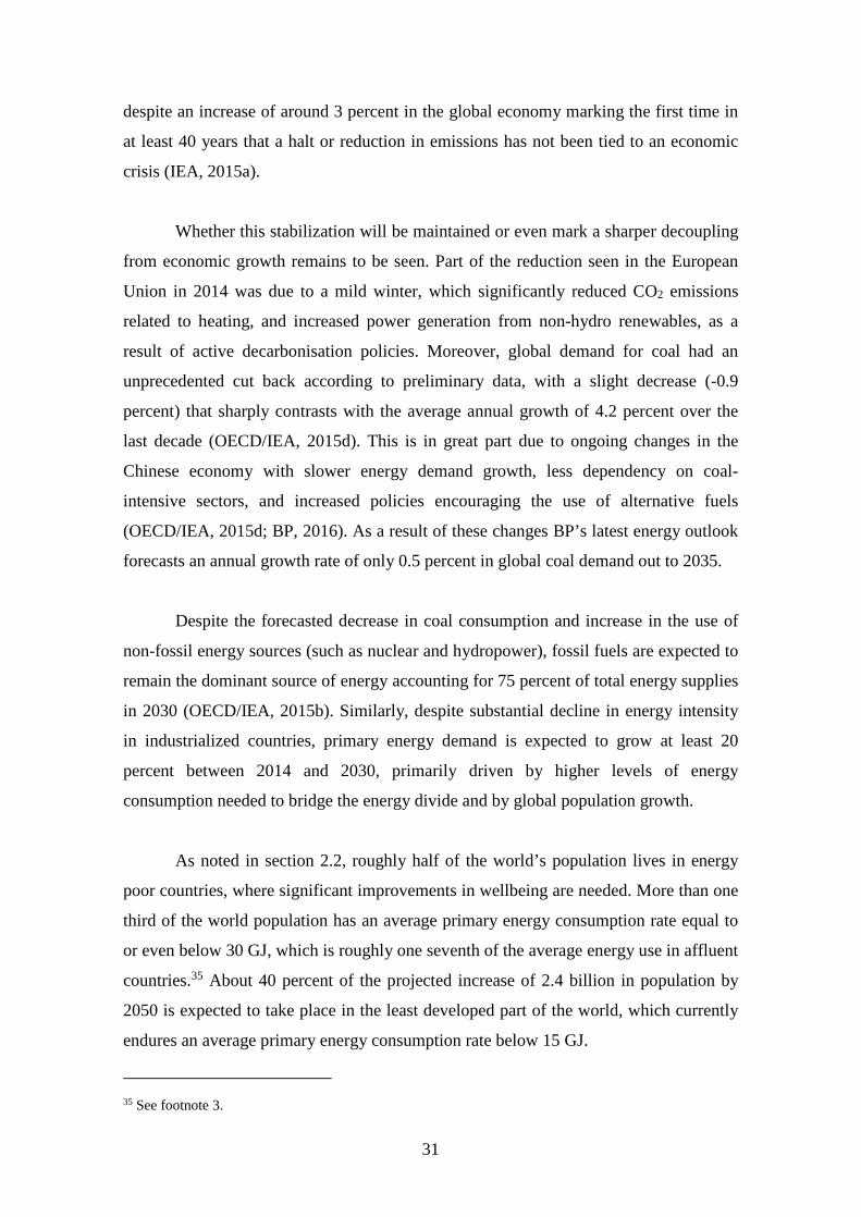
31

despite an increase of around 3 percent in the global economy marking the first time in

at least 40 years that a halt or reduction in emissions has not been tied to an economic

crisis (IEA, 2015a).

Whether this stabilization will be maintained or even mark a sharper decoupling

from economic growth remains to be seen. Part of the reduction seen in the European

Union in 2014 was due to a mild winter, which significantly reduced CO2 emissions

related to heating, and increased power generation from non-hydro renewables, as a

result of active decarbonisation policies. Moreover, global demand for coal had an

unprecedented cut back according to preliminary data, with a slight decrease (-0.9

percent) that sharply contrasts with the average annual growth of 4.2 percent over the

last decade (OECD/IEA, 2015d). This is in great part due to ongoing changes in the

Chinese economy with slower energy demand growth, less dependency on coal-

intensive sectors, and increased policies encouraging the use of alternative fuels

(OECD/IEA, 2015d; BP, 2016). As a result of these changes BP’s latest energy outlook

forecasts an annual growth rate of only 0.5 percent in global coal demand out to 2035.

Despite the forecasted decrease in coal consumption and increase in the use of

non-fossil energy sources (such as nuclear and hydropower), fossil fuels are expected to

remain the dominant source of energy accounting for 75 percent of total energy supplies

in 2030 (OECD/IEA, 2015b). Similarly, despite substantial decline in energy intensity

in industrialized countries, primary energy demand is expected to grow at least 20

percent between 2014 and 2030, primarily driven by higher levels of energy

consumption needed to bridge the energy divide and by global population growth.

As noted in section 2.2, roughly half of the world’s population lives in energy

poor countries, where significant improvements in wellbeing are needed. More than one

third of the world population has an average primary energy consumption rate equal to

or even below 30 GJ, which is roughly one seventh of the average energy use in affluent

countries.35 About 40 percent of the projected increase of 2.4 billion in population by

2050 is expected to take place in the least developed part of the world, which currently

endures an average primary energy consumption rate below 15 GJ.

35 See footnote 3.

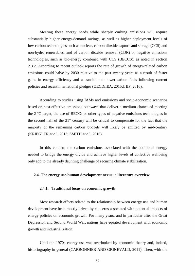
32

Meeting these energy needs while sharply curbing emissions will require

substantially higher energy-demand savings, as well as higher deployment levels of

low-carbon technologies such as nuclear, carbon dioxide capture and storage (CCS) and

non-hydro renewables, and of carbon dioxide removal (CDR) or negative emissions

technologies, such as bio-energy combined with CCS (BECCS), as noted in section

2.3.2. According to recent outlook reports the rate of growth of energy-related carbon

emissions could halve by 2030 relative to the past twenty years as a result of faster

gains in energy efficiency and a transition to lower-carbon fuels following current

policies and recent international pledges (OECD/IEA, 2015d; BP, 2016).

According to studies using IAMs and emissions and socio-economic scenarios

based on cost-effective emissions pathways that deliver a medium chance of meeting

the 2 oC target, the use of BECCs or other types of negative emissions technologies in

the second half of the 21st century will be critical to compensate for the fact that the

majority of the remaining carbon budgets will likely be emitted by mid-century

(KRIEGLER et al., 2013; SMITH et al., 2016).

In this context, the carbon emissions associated with the additional energy

needed to bridge the energy divide and achieve higher levels of collective wellbeing

only add to the already daunting challenge of securing climate stabilization.

2.4. The energy use-human development nexus: a literature overview

2.4.1. Traditional focus on economic growth

Most research efforts related to the relationship between energy use and human

development have been mostly driven by concerns associated with potential impacts of

energy policies on economic growth. For many years, and in particular after the Great

Depression and Second World War, nations have equated development with economic

growth and industrialization.

Until the 1970s energy use was overlooked by economic theory and, indeed,

historiography in general (CARBONNIER AND GRINEVALD, 2011). Then, with the

33

advent of the oil crisis in the 1970s, rising concerns about costs and resource scarcity

brought energy to the forefront of domestic and foreign policies, prompting questions

on whether and how energy consumption affected economic growth. Aiming at better

guiding policy makers on energy conservation policies and their potential impacts on

the economy, many studies started to empirically analyze the relationship between

energy and development by testing for causality between energy use and economic

growth, typically measured by GDP.

The needed knowledge base started to be built with KRAFT AND KRAFT

(1978), followed by a wealth of studies using various econometric approaches

(including Granger causality tests, error correction model, cointegration, vector

autoregression, and panel data analysis), covering different groups of countries and

development stages, as well as, different time periods, spanning from as early as 1947

until 2011, as shown in Appendix A. An overview of these studies reveals that the use

of different time span, set of countries, data sources, and econometric methods have

resulted in diverse outcomes (CHONTANAWAT et al., 2008; HUANG et al., 2008;

OZTURK, 2010; CHEN et al., 2012; MENEGAKI, 2014).

KRAFT AND KRAFT (1978) explored the causal relationship between gross

national product and energy consumption using annual data for the United States over

the period 1947-1974, and their results suggest that there is a uni-directional causal

relationship from economic growth to energy consumption. However, a subsequent

research (AKARCA AND LONG, 1979) using the same data over different time

periods obtained different results. Estimation methodologies also proved to be a

relevant factor in the diverging results found in further studies (AKARCA AND LONG,

1980; YU AND HWANG, 1984; YU AND CHOI, 1985; EROL AND YU, 1987a,

1987b; YU AND JIN, 1992; cited in HUANG et al., 2008).

According to CHONTANAWAT et al. (2008), a large number of studies were

based upon the ‘Granger-causality’ principle (GRANGER, 1969 and SIMS, 1972).

However, the majority covered only data from the United States or, at most, a small

group of developed countries between the 1940s and the 1980s. Another group of

studies used cointegration and the error correction model (GRANGER, 1988) using also

data from some developing countries from the 1950s through the early 2000s. Yet,

34

another set of studies used the HSIAO (1981) technique, which enhances Granger-

causality by incorporating the use of AKAIKE (1970) ‘final prediction error’ (FPE)

criteria on data from the U.S., Latin America and several Asian countries over the

period between 1940s and the early 2000s.

Subsequent studies include multivariate analyzes encompassing other variables

besides economic growth and energy consumption, in spite of data limitations. For

instance, HALICIOGLU (2009) and ZHANG AND CHENG (2009) included foreign

trade and urban population in addition to economic growth and energy consumption in

their analyses. More recent multivariate analyses have included CO2 emissions into

their modeling frameworks (SOYTAS et al., 2007; APERGIS AND PAYNE, 2009;

SOYTAS AND SARI, 2009; ZHANG AND CHENG, 2009; PAO AND TSAI, 2010;

CHANG AND CARBALLO, 2011; AROURI et al., 2012; and OMRI, 2013), primarily

because climate change policies commonly entail energy conservation policies, which

can potentially impact economic growth. Even though most of these studies concluded

that energy consumption is often a key determinant of increased CO2 emissions, the

outcome of their empirical results have also been inconsistent, as shown in Appendix A.

Notwithstanding the inconsistency in findings, the relationship between energy

consumption and economic growth has been primarily described as one of the following

four competing hypotheses in those studies:

i. The neutrality hypothesis refers to the absence of a causal relationship

between energy consumption and economic growth, i.e. the two variables are

unrelated. In this case, other factors, besides economic growth, directly or

indirectly affect energy consumption, and vice-versa.

ii. The conservation hypothesis refers to a uni-directional causality from

economic growth to energy consumption, i.e. economic growth leads to

increased energy consumption with no feedback.

iii. The growth hypothesis refers to a uni-directional causality from energy

consumption to economic growth, means that energy can be considered as a

limiting factor, or essential input, to economic growth.

35

iv. The feedback hypothesis refers to a bi-directional causality between energy

consumption and economic growth, implying that energy consumption and

economic growth are jointly determined and affected at the same time.

The policy implications of some of these hypotheses can be significant. Studies

that have found the energy-GDP nexus prescribed under the growth hypothesis argue

against reductions in energy consumption due to its adverse impact on GDP and support

increases in energy consumption as a potential contributor to economic growth.

Similarly, in the feedback hypothesis, any restriction on energy use would impede

economic growth. In contrast, energy conservation policies would only be encouraged

under the neutrality or conservation hypotheses.

CHONTANAWAT et al. (2008) conducted a systematic review combining

statistical methods and using IEA data on 100 countries over the period from 1965 to

2000 and concluded that causality running from energy consumption to economic

growth occurs more often in OECD/developed countries than in non-OCDE/developing

ones. Therefore, according to this study, energy conservation policies should not be

pursued in OECD/developed countries, as they would likely have an impact on their

economic growth.

Meanwhile, another study published one month later (HUANG et al., 2008)

presents an analysis with a similar number of countries (eighty-two countries split in

four income groups) using panel data from 1972 to 2002, and does not find any

evidence indicating that energy consumption leads to economic growth in the high

income group (i.e. OECD/developed countries). Hence, HUANG et al., (2008)

encourage stronger energy conservation policies in these countries. Notably, according

to both studies, energy conservation policies would not have a significant impact on the

GDP of the developing world.

CHEN et al. (2012) observed that the different results found in the literature

may have been caused by factors such as the use of distinct subject selections (including

GDP and energy consumption), time spans, econometric approaches and/or other

explanatory variable selections. In an attempt to help understand the controversial and

inconsistent empirical results found in the literature, they prepared a comprehensive

36

study on this issue based on a detailed literature review using a meta-analysis and a

multinomial logit model. They used 174 samples from 39 studies found in the literature

that test the relationship between energy consumption and economic growth to help

determine how this relationship is affected by those factors. The dependent variables

consisted of the four competing hypotheses on the relationship between energy

consumption and economic growth. The independent variables included the socio-

economic characteristics, research target characteristics and estimation methods.

Their findings suggest that if the data sets cover the period after the year 2000

the growth hypothesis will be the most likely outcome over the other three types.

Conversely, there is no predominant hypothesis if the data sets cover the 1960s. Thus,

showing that different time periods used in testing the relationship between energy

consumption and economic growth affect the empirical results differently. Similarly, the

use of the Granger-causality test tends to infer the feedback hypothesis, while the use of

other estimation methods tends to imply the neutrality hypothesis. Moreover, data sets

comprised of developed countries tend to result in the conservation hypothesis, whereas

those comprised of developing countries tend to infer the growth hypothesis. Thus,

denoting that different econometric approaches and/or levels of economic development

of the countries selected will affect the results differently as well.

Despite the inconclusive results on the direction of econometric causality

between energy consumption and economic growth, the scientific community seems to

have reached a consensus that energy is a critical factor for economic development

(OECD, 2013; FIZAINE AND COURT, 2016).

2.4.2. Recent interest in broader aspects of human development

Concerted international efforts towards global sustainability since the adoption

of the Millennium Declaration (UNGA, 2000) by 189 heads of states in 2000 have led

research efforts related to energy consumption and economic growth to include broader

aspects of human development. PASTERNAK (2000), SMIL (2003), DIAS et al.

(2006), MARTINEZ AND EBENHACK (2008), JACKSON (2009), STEINBERGER

AND ROBERTS (2009, 2010), SMIL (2010b), COSTA et al. (2011), MAZUR, (2011),

PASTEN AND SANTAMARINA (2012), RAO AND BAER (2012), STEINBERGER

37

et al. (2012), JORGENSON (2014), STECKEL et al. (2013), UGURSAL (2014), and

LAMB AND RAO (2015) all use the Human Development Index (HDI) or its

components as proxy measures for human development beyond the economic

dimension in their analyse of the link between energy consumption and human

development.

HDI is a measure of human development that combines proxies for three

important human capabilities: health (represented by life expectancy), education

(represented by literacy and school enrollment), and a decent standard of living

(represented by GDP per capita).36 The HDI was introduced by the United Nations

Development Programme (UNDP) in 1990 as an alternative to address some of the

shortcomings of Gross National Product (GNP) (STANTON, 2007) (see section 3.3.2

below). Among other limitations, GNP was unable to inform on the quality of life of the

people. As such, HDI has been consistently used as a reference metric to compare social

and economic development within and between countries across time (COSTA et al.,

2011). It uses readily accessible source of data across 187 countries and is based on a

reasonably consistent basis since 1990 (UNDP, 2013).

Interestingly, most of these studies have found strong correlations between

energy consumption and/or CO2 emissions and HDI levels in developing countries, but

a decoupling pattern in industrialized countries, as improvements in quality of life start

to level off at a certain saturation level. An important take away from these results is the

understanding that while increased energy consumption is bound to increase economic

growth, and CO2 emissions into the atmosphere, it may not necessarily improve human

development after societies have reached a certain level of economic development and

quality of life, including adequate housing, ample food supply and clean water, decent

transportation, and good indicators of health and education.

This saturation or threshold phenomenon is well examined in MAX-NEEF

(1995), PASTERNAK (2000), MARTINEZ AND EBENBACK (2008), JACKSON

36 The indices are relative and normalized, such that each component is calculated with respect to the minimum value in the sample, and then normalized to the maximum difference found in the sample. A country potentially having the highest score across all three dimensions would have an HDI value of 1.0.

38

(2009), STEINBERG AND ROBERTS (2009 AND 2010), SMIL, (2010B), MAZUR,

(2011), and PÎRLOGEA (2012). It is also depicted in the regression curves in Figure 9

below. For countries with low or medium HDI rankings (developing countries), slight

increases in energy consumption and carbon emissions translate into significant

improvements in human development; hence a strong, positive, and roughly linear

relationship is observed. Meanwhile, for countries with higher HDI rankings (mostly

industrialized countries) after a modest threshold is reached, it takes significant

increases in energy consumption and carbon emissions to make further improvements in

human development, if any.

Moreover, this point of inflection has been equated to a threshold level

equivalent to approximately 105 GJ per capita primary energy consumption in

PASTERNAK (2000), MARTINEZ AND EBENHACK (2008), and UGURSAL

(2014). PASTERNAK (2000) and UGURSAL (2014) have estimated a range from 378

to 492 EJ of overall energy needed to reach such threshold level globally.37 According

to PASTERNAK (2000) this threshold would be achieved in 2020 while, according to

UGURSAL (2014), it would be achieved only by 2100. Other ideal levels have been

determined based on average GDP per capita, HDI, basic needs access, and life

expectancy (COSTA et al., 2011; UGURSAL, 2014; and LAMB AND RAO, 2015).

37 This range refers to achieving a minimum of 4,000 kWh (or 14.4 GJ) per capita electricity consumption or an estimated (at 7.5 ratio) 108 GJ (or 2580 koe) per capita primary energy consumption.

39

Figure 9 - Saturation and decoupling trend between HDI and carbon emissions (upper

plot, 115 countries) and between HDI and energy consumption (114 countries for 1990

data and 116 countries for 2000 data and 2010 data) from 1990 to 2010.

Source: Adapted from STEINBERGER AND ROBERTS, 2010 using data from the World

Development Indicators (WORLD BANK, 2016) and the Human Development Report 2013

(UNDP, 2013).

The regression curves in Figure 9 also show that for constant energy

consumption and corresponding carbon levels, HDI increased overtime time. For

40

instance, for 2 tons of carbon per capita the expected HDI levels would be 0.712, 0.768,

and 0.809 for 1990, 2000, and 2010, respectively. This implies that overall human

development has been slowly decoupling from carbon emissions overtime, in other

words, becoming somewhat more carbon-efficient as observed in STEINBERGER

AND ROBERTS (2009 and 2010) and STEINBERGER et al. (2012).

In theory, technological improvements could explain part of this decoupling

trend as more energy services are delivered per unit of input energy. However, in

practice, the growth of energy efficiency is more than matched by growth in energy

consumption as a result of rebound effects, a phenomenon otherwise known as the

“Jevon's Paradox” (GREENING et al., 2000; AYRES et al., 2007; SORRELL, 2007).38

An example of a rebound effect would be the driver who replaces a car with a fuel-

efficient model, only to take advantage of its cheaper running costs to drive further and

more often (SORRELL, 2007). DALY (2013) argues that such rebound effects would

be avoided if efficiency were to be sought alongside throughput limitation.

STEINBERGER et al. (2012) and JORGENSON (2014) further demonstrate

that this decoupling is remarkably steady albeit at highly differentiated trajectories when

individual countries are taken into account, given their highly differentiated states of

carbon emissions and life expectancy. JORGENSON (2014) shows that in some

countries the level of anthropogenic carbon emissions per unit of human development

(measured in terms of average life expectancy at birth) did not reduce overtime (e.g.

Kenya) and has in fact increased during either part of or the whole period between 1970

and 2009 (e.g. China and Australia), which is in part explained by changing effects of

per capita GDP on such levels (measured in terms of elasticity coefficients). Another

contributing factor is the change in decarbonisation rates (rate at which the carbon

emissions associated with each unit of GDP decreases) experienced by each nation,

which is in turn driven by changes in the energy intensity of the economy (or energy use

per unit of GDP) and changes in the carbon intensity of the energy supply (or carbon

emissions per unit of energy).

38 The “Jevon’s paradox” states that productivity increases, in the end, do not result in resource savings but in accelerated economic growth: “with fixed real energy prices, energy efficiency gains will increase energy consumption above what it would be without these gains” (SAUNDERS, 1992).

41

However, because they used the HDI or its components as proxy measures for

human development or wellbeing, and even though carbon emissions are included in

their analyses, current studies on the relationship between energy consumption and

human development have yet to encompass the ecological dimension and the

intergenerational equity principle, which are critical for achieving sustainable

development.

In spite of existing knowledge of the so-called externalities (e.g. MARSHALL,

1890 and PIGOU, 1920), or unintended and uncompensated effects upon others

resulting from consumption or production activities as defines in PERMAN et al.

(2003), there was hope of a limitless, energy-intensive economic development model.

Aiming for unending economic growth is not sustainable in a world with environmental

limits. In fact, humanity’s imprint on the global environment through resource use and

waste production may have exceeded the regenerative and absorptive capacity of the

biosphere (BARNOSKY et al., 2012; ROCKSTRÖM et al., 2009; STEFFEN et al.,

2011), thus compromising the ability of future generations to ensure their wellbeing.

The perception of natural resources and the environment has shifted from a

vision of being a limit to economic growth to having an active role in reducing poverty,

achieving higher living standards and increasing human development levels. Everything

that humanity needs for survival and wellbeing depends, either directly or indirectly, on

the natural environment. Humans are part of the natural world and dependent on the use

of natural resources to sustain their social and economic wellbeing.

There is evidence that although man-made changes to ecosystems have helped to

improve the lives of billions, they are increasing the likelihood of non-linear and

potentially abrupt changes in ecosystems (e.g. fisheries collapse, climate change,

disease emergence), with important consequences for human wellbeing (HARRIS,

2012). These changes have weakened nature’s ability to deliver key ecosystem services

such as purification and waste treatment, air quality maintenance, biological control,

storm protection, climate regulation, and regulation of human diseases.39 Data shows,

39 For an overview of the condition and trends in the world’s ecosystems and services refer to the United

42

for instance, that progress in HDI has come at the cost of global warming (TOGTOKH,

2011).

In an attempt to better understand the relationship between the pressure placed

on the environment and improvements in human wellbeing, several recent studies have

begun to explore the different ecological/environmental intensities of wellbeing (EIWB)

of countries (DIETZ et al., 2007, 2009, 2012; KNIGHT AND ROSA, 2011; KNIGHT

et al., 2013). They define EIWB as the ratio between a measure of stress on the

environment, such as the ecological footprint or GHG emissions, and a measure of

human wellbeing, typically life expectancy at birth, one of the components of HDI.

As discussed in the following section, the concept of human development has

long evolved to incorporate the notion of sustainability setting the stage to a new

paradigm of development, which emphasizes the importance of sustaining all forms of

resources (e.g. physical, human, financial and environmental) as a precondition for

meeting the needs of both current and future generations as well. Under this new

development paradigm sustainability is to be achieved by focusing on economic growth,

social equity, and environmental protection (WCED, 1987). Interestingly, evidence

from STEINBERGER et al. (2012) suggests that nations can achieve environmental and

social sustainability (in the form of lower carbon emissions and high life expectancy),

but only below a given cap of per capita income ($12,000 USD).

While Human Development reports, where the HDI is published annually,

discuss the importance of sustainability and the avoidance of environmental degradation

and even present various ancillary indicators on the consumption of natural resources,

the headline indicator is still the HDI (MORSE, 2003). In order to fully become a

measure of sustainable development, the HDI would have to be revised to incorporate

resource exploitation and environmental degradation (DESAI, 1995; SAGAR AND

NAJAM, 1998; NEYMAYER, 2001; MORSE, 2003).40 Otherwise, the HDI will

continue failing to represent all three dimensions of sustainable development - social,

Nations 2005 Millennium Ecosystem Assessment, the result of a four-year (2001-2005) study involving more than 1,300 experts worldwide. 40 Surprisingly, despite the international attention drawn towards sustainable development during the late 1980s and particularly following the Rio Earth Summit in 1992, there have been few calls to ‘green’ the HDI (NEUMAYER, 2001).

43

economic, and environmental.

To the author’s knowledge there has been no study on the relationship between

energy use and human development or wellbeing that uses a measure of the latter that

encompasses all three dimensions of sustainable development as a single value,

expressed in monetary terms. Possibly, because in order to examine such relationship it

is essential to first understand the underlying concepts and dimensions of the new

development paradigm, where the goal of economic growth has been replaced by that of

human wellbeing, as discussed in greater detail in the next section.

44

3. Human wellbeing: concepts and measurements from a development

perspective

According to the mainstream economic theory, economic growth is the result

from the accumulation of factors of production, particularly capital and labor, and from

increased productivity (DORNBUSCH et al., 1998). By assuming a high degree of

substitutability between factors of production, economic growth is viewed as unlimited

(DALY, 2007). In disagreement with this view, ecological economists argue that

economic growth reflects the quantitative physical increase in the matter-energy

throughput that begins with depletion and ends with pollution (DALY, 2013). As such,

economic growth is but a narrow aspect of human development within the energy-

development nexus. Human development, in contrast, is associated with the qualitative

improvement in the capacity of a given throughput to provide for the maintenance and

enjoyment of life in general (DALY, 2013), i.e. human wellbeing.41

Human wellbeing from a development perspective has become an important

area for policy as it accounts for elements in human life that cannot be defined,

explained, or primarily influenced by economic growth (MCALLISTER, 2005).

However, as discussed in section 2.4.2 above, it was not until around the year 2000 that

studies assessing the relationship between energy consumption and development started

to include other variables besides economic growth and use proxy measures for human

development beyond the economic dimension. This change can be primarily attributed

to growing worldwide concern and interest in sustainability, which is mostly described

as the requirement to maintain the capacity to provide non-declining wellbeing over

time (NEUMAYER, 2004).

While there has been broad consensus on the need to replace the goal of

economic growth with that of human wellbeing as the ultimate purpose of human

development, it is not clear what it is or how it should be measured, neither at the

individual level or that of a society as a whole (MCGILLIVRAY AND CLARKE,

41 Even though the literature often uses the terms ‘‘happiness’’, ‘‘wellbeing’’, ‘‘quality of life”, and “life satisfaction” interchangeably (MCALLISTER, 2005), in this study we refer to ‘‘wellbeing’’ in the context of societal welfare, unless otherwise indicated.

45

2006; CANOY AND LERAIS, 2007; DODGE et al., 2012; KING et al., 2014). Human

wellbeing cannot be directly observed, making it an ambiguous and abstract concept

primarily used to refer to whatever is assessed in an evaluation of a person’s situation

with focus on the quality of the person’s ‘being’ (GASPER, 2005; MCGILLIVRAY,

2005; MCGILLIVRAY AND CLARKE, 2006). As a result, there is a wide range of

conceptual approaches to it in the literature, partly reflecting different contexts,

purposes, and areas of concern (see DASGUPTA, 2001; GASPER, 2004; STIGLITZ et

al., 2009; and ADLER AND SELIGMAN, 2016).

This chapter discusses the challenges associated with trying to define and

measure wellbeing from a human development perspective, given its complex and

multi-dimensional nature. It shows how even though massive efforts are still needed to

arrive at a unified theoretical foundation around human wellbeing, the host of

conceptual approaches developed to date have increased awareness and recognition of

the combined effects of social equity and environmental protection, alongside economic

growth on the achievement of collective wellbeing.

3.1. Early conceptualizations: from material individualism to spiritual

collectivism

In order to help better understand the multitude of present-day interpretations of

wellbeing, this section renders an overview of dominant conceptual approaches to

human wellbeing, which can be traced back as far as ancient Greek philosophical

traditions that are founded on distinct views of human nature and of what constitute a

good society: hedonia and eudaimonia (RYAN AND DECI, 2001; MCALLISTER,

2005; RYFF AND SINGER, 2008). The hedonic conception focuses on happiness and

self-satisfaction and defines wellbeing in terms of pleasure attainment and pain

avoidance. The eudaimonic conception, in turn, focuses on meaning and self-realization

and defines wellbeing in terms of actualization of human potentials, i.e. well-considered

fulfillment (RYAN AND DECI, 2001). Moreover, in order to make the conceptual

analysis more comprehensive, it attempts to make a parallel with other significant

conceptualizations present in Eastern philosophical and cultural traditions.

46

3.1.1. Hedonism: wellbeing as maximization of individual pleasure

Aristippus, a Greek philosopher from the fourth century BCE who founded the

Cyrenaic school, believed that the ultimate purpose of human life was to experience as

much pleasure as possible while generally avoiding any painful experiences (RYAN

AND DECI, 2001). From his perspective, maximizing one’s pleasurable moments was

the ultimate goal of human life. Wellbeing from a hedonic approach is, therefore,

primarily associated with self-satisfaction. Hedonism42 has been expressed in many

forms throughout history, varying from a relatively narrow focus on bodily pleasures to

a broad focus on appetites and self-interests, as well as valued outcomes in varied

realms (RYAN AND DECI, 2001).

In view of its inconsistencies with military nobility and Christian virtues,

hedonism received little attention by scholars and was mostly perceived as a derogatory

idea during the Roman Empire and the Middle Ages until Pierre Gassendi (1592–1655),

who reinterpreted the concept of pleasure in a distinctly Christian way (MOEN, 2015).

Gassendi’s work influenced many other Enlightenment thinkers, particularly Thomas

Hobbes and John Locke. However, modern history of hedonistic theories is said to start

with the work of Jeremy Bentham (MOEN, 2015), considered the founding father of

utilitarianism (HIRSCHAUER et al., 2015).

Drawing on the fundamental principles of hedonism, Jeremy Bentham

(BENTHAM, 1789) argued that not only human behavior is motivated by pleasure and

pain, but their net satisfaction translates into “utility.” According to his propositions,

society’s wellbeing would be the sum of these utilities, such that an ethical course of

action was that which led to “the greatest happiness for the greatest number”

(STANTON, 2007). Bentham further believed the value of pleasure to be its intensity

multiplied by its duration and to not contain any qualitative difference. Later

utilitarians, like J. Stuart Mill, argued that there could be qualitative differences, in

particular between “higher” and “lower” levels of pleasure (see NUSSBAUM, 2007).

Modern hedonists tended also to think in terms of general good and universal

42 The word “hedonism” derives from the Greek word “hedone” (“pleasure”) (MOEN, 2015).

47

ends, in contrast to the more egoistic form taken by the ancient Greeks. Henry Sidgwick

(1838-1900), in particular, when defining utilitarianism equated it to universalistic

hedonism, which directed the individual to act in a way that promoted the happiness of

all individuals, as opposed to egoistic hedonism (see SIDGWICK, 1981 [1874], Book

IV, Chapter 1, Section 1, p. 200).

Under utilitarianism, or universalistic hedonism, wellbeing was reduced to

pleasure and further reduced to the scalar of unitary pleasure or utility (GASPER,

2004), which could in principle be summed across individuals to determine societal

wellbeing. However, in the absence of inter-personal comparability, the utility of

individuals cannot be aggregated, nor can it be compared in order to consider

distribution (STANTON, 2007). Nevertheless, utilitarianism has been the dominant

approach to human wellbeing used in mainstream economic theory since the 1930s

(STANTON, 2007).

3.1.2. Eudaimonism: wellbeing as the actualization of human potentials

Not in agreement with Aristippus' hedonic approach, Greek philosopher

Aristotle (384 to 322 BCE) proclaimed that living a life of contemplation and virtue, in

accordance with one’s inherent truth was the pathway to true happiness and wellbeing

(NORTON, 1976; cited in RYFF AND SINGER, 2008). Accordingly, eudaimonia43

was “activity expressing virtue” and all that human desires and actions aimed to

achieve, and that it was something generated by our actions and not our belongings

(STANTON, 2007). Aristotle did not denigrate hedonic pleasure per se, but rather, the

pursuit of hedonic pleasure purely for pleasure’s sake (WATERMAN, 2008). Given that

such behavior would be contrary to his interpretation of virtue, i.e. a state of character

concerned with finding the middle ground between excess and deficiency (RYFF AND

SINGER, 2008).

In one of his most influential works, the Nicomachean Ethics (ARISTOTLE,

1985 [350 BCE]), while seeking to answer what would be the ultimate purpose of 43 The term "eudaimonia" is a classical Greek word, consisting of "eu" ("good") and "daimōn" ("spirit"). It is traditionally translated as happiness but many philosophers, religious masters, and visionaries have denigrated happiness per se as a principal criterion of wellbeing (RYAN AND DECI, 2001).

48

human existence, Aristotle presented a theory of wellbeing that is still relevant today.

According to him, wellbeing consisted in achieving, through the course of a whole

lifetime, the best that is within us, i.e. all the goods that lead to the perfection of human

nature and to the enrichment of human life. Aristotle was clearly not concerned with the

subjective states of wellbeing. Rather, his conception of the highest good towards which

we all should be reaching was the task of self-realization, played out individually, each

according to his or her own disposition and talent (RYFF AND SINGER, 2008).

According to eudaimonism, individuals have the responsibility to recognize and

live in accordance with one’s true self (daimōn) (BANAVATHY AND CHOUDRY,

2014). The daimōns refer to the potentialities of each person, the realization of which

represents the greatest fulfillment. Eudaimonic advocates argued that living a life of

virtue, and actualizing one’s inherent potentials was the way to wellbeing. Eudaimonia,

thus, incorporates the essence of the two great Greek imperatives: first, to ‘‘know

thyself’’ (a phrase inscribed on the temple of Apollo at Delphi), and second, to ‘‘choose

yourself’’ or ‘‘become what you are’’ (NORTON, 1976; cited in RYFF AND SINGER,

2008).

Eudaimonic theorists cautioned that not all sources of pleasure foster wellbeing.

Instead, they argued that it is the realization of human potential, rather than simply life-

satisfaction, that is central to wellbeing (RYAN AND DECI, 2001; MCALLISTER,

2005). In this sense wellbeing cannot be equated merely to a sensation of happiness.

Human beings have more faculties than just feeling happiness, pleasure or pain, notably

they are creatures of reasoning and of meaning-making, of imagination, and of intra-

and inter-societal links and identities (GASPER, 2004).

3.1.3. Eastern conceptualizations: wellbeing through self-transcendence

Questions regarding the essential qualities of a good society and the good life

have also captured the minds of great thinkers across Eastern traditions (RYFF AND

SINGER, 2008; BANAVATHY AND CHOUDRY, 2014; JOSHANLOO, 2014). The

conceptual approaches to wellbeing in Eastern philosophies can also be traced back to

ancient times, to the age of Confucius (c. 551 to 472 BCE) in China (ZHANG AND

VEENHOVEN, 2008) and to the Vedic and Upanishadic periods (c. 3000 to 1000 BCE)

49

in India (SALAGAME, 2003; BANAVATHY AND CHOUDRY, 2014). As discussed

below, except for India’s school of materialist philosophy, eastern conceptualizations of

wellbeing are more consistent with the eudaimonic perspective of western theorists. In

fact, they go beyond the proposition of the latter, suggesting that collective wellbeing

can only be achieved by de-emphasizing individualistic virtues and, ultimately, by

cultivating spirituality and self-transcendence.

Confucianism is believed to be at the root of the traditional schools of thoughts

in eastern traditions (JOSHANLOO, 2014). Similar to the Greek eudaimonia, this

ancient philosophy associates wellbeing with achieving a good life, one of virtue, honor,

and purpose. Confucius was not so much concerned with the individual wellbeing but

how we relate collectively to each other in all contexts. The pivotal idea of

Confucianism is ‘Jen’, a feeling of compassion, i.e. concern for the wellbeing of others

(ZHANG AND VEENHOVEN, 2008).

The other two major Chinese traditions, Taoism and Buddhism, differed in how

they valued life (ZHANG AND VEENHOVEN, 2008), however, they were also wary

of bodily pleasures, and promoted instead desire control techniques to keep individuals

from pursuing pleasures at the expense of ignoring main virtues (IP, 2011;

JOSHANLOO, 2014). Moreover, suffering and negative emotions not only are not

considered entirely bad in these cultures, but are thought to contribute to spiritual

development.

Indian traditions, in turn, convey three general perspectives on wellbeing: the

hedonistic perspective, the transcendent perspective, and the collectivistic perspective

(SALAGAME, 2003). These can be associated with the perception of human evolution

through a progressive expansion of consciousness as different layers (sheaths) that

represent dimensions of awareness which unfold towards a state of realization of one’s

transcendent Self (Ātman), i.e. true wellbeing (swasthya) and welfare (kalyana). As

such, human beings are believed to transition out of the hedonistic approach to

wellbeing through degrees of the collectivistic approach towards the transcendent

approach to it as they climb up the evolutionary ladder.

Under the hedonistic perspective, fulfillment of desires, particularly of sensory

50

nature, is the sole criterion towards securing wellbeing. This approach was followed by

India’s school of materialist philosophy, originally called Lokāyata (“prevalent in the

world”, Sanskrit lokeṣu āyatam, “widespread among the people”) (BHATTACHARYA,

2009), which was founded around the same time that materialism developed

independently in ancient Greece or perhaps slightly before (WOJCIEHOWSKI, 2015).

According to this school of thought, pleasure was asserted as the highest good,

and the only reasonable way to enjoy one’s life. It rejected the notion of God, dharma

(values), law of karma (theory of action leading to rebirth), objective ethical laws, and

many other ideas associated with the Vedas (the orthodox traditional wisdom of India)

and the spiritualistic schools of Eastern philosophy (e.g. Jainism, Buddhism, Hinduism).

Likely this was one of the main reasons it never gained prominence in Eastern

philosophies and cultures, although SALAGAME (2003) argues that it is taking hold of

the Indian psyche in contemporary times due to westernization and globalization.

Another reason lies on the fact that the hedonistic conceptualization not only promotes

the pursuit of pleasures at the expense of ignoring main virtues, the cornerstone of

achieving the highest good in Eastern cultures, but also the cultivation of self-

centeredness, which does not accord with the core values and ethos of collectivistic

societies (JOSHANLOO, 2014).44 While the Vedic tradition does not indorse the

hedonistic approach to wellbeing, it does not negate the role and necessity of this aspect

of pleasurable experience or materialistic happiness (viṣayānanda) (BANAVATHY

AND CHOUDRY, 2014).

Lying on the opposite side of the spectrum, the second perspective on wellbeing,

upheld by most traditional Indian philosophers, is rooted in the transcendental view of

reality, according to which the ideal wellbeing is understood as the realization of one’s

transcendent Self (Ātman) (SALAGAME, 2003). Transcendental happiness

(Brahmānanda) is regarded as the highest form of happiness that a person can

experience. It is transcendental in the sense that it transcends the limitations of

compartmentalized individual existence (BANAVATHY AND CHOUDRY, 2014).

44 Wellbeing conceptualizations are to a great extent associated with the way the ‘self’ is perceived. A conspicuous difference between western and eastern traditions lies on the fact that the former define the ‘self’ primarily based on the ideals of individualism, while the latter tend to regard it as a part of the collective (JOSHANLOO, 2014).

51

Similar to the eudaimonic perspective in western traditions, it fosters the realization of

one’s inherent potentials as the way towards securing wellbeing.

However, self-realization is qualitatively different from the self-actualization

advocated by eudaimonic theorists (BANAVATHY AND CHOUDRY, 2014). Also

contrary to the views of eudaimonic theorists, the transcendent perspective advocates

that one does not need to interact with any external object, situation or person in order

to fulfill his or her potentials (BANAVATHY AND CHOUDRY, 2014). It starts from

the presumption that human beings have intrinsic happiness and contentment within

them, waiting to be discovered. Moreover, it is based on an all-encompassing universal

vision that aspires for the wellbeing of everyone (SALAGAME, 2003). The causes,

determinants and correlates of this kind of conceptualization cannot be equated with any

western conceptualization (BANAVATHY AND CHOUDRY, 2014).

The third and last Indian perspective on wellbeing, the collectivistic one, lies in

between the two perspectives described above. Similar to eudaimonia, it refers to an

aspect of happiness derived from the actualization of one’s best potentials (kāvyānanda)

(BANAVATHY AND CHOUDRY, 2014). It acknowledges the numerous differences

in the needs and aspirations of people, and the fact that the majority of people have an

intermediary approach to life between a purely hedonistic approach and a more spiritual

one (SALAGAME, 2003).

3.2. Modern conceptualizations: from economic growth to sustainability

Interest in the wellbeing of people and nations has been central to economists

from the founders of modern economics (e.g. Adam Smith, David Ricardo, John Stuart

Mill, and Karl Marx) to contemporary economists, such as Paul Streeten, Amartya Sen,

Martin Ravallion and Ravi Kanbur (SUMNER, 2004), who have broken away from the

utilitarian concept, while viewing wellbeing as a multi-dimensional construct.45 It is

noteworthy, however, that by the end of the 20th century, despite ‘rigorous and elegant

45 Despite the differences between the hedonistic and eudaimonic approaches, most researchers now believe that wellbeing is a multi-dimensional construct (e.g. DIENER, 2009; STIGLITZ et al., 2009; cited in DODGE et al., 2012) and that the two approaches to the study of wellbeing are not mutually contradictory (KASHDAN et al., 2008).

52

in its logic’, mainstream economics was still uncertain about the implications of policies

on human wellbeing (ACKERMAN et al., 1997).

As the 21st century unfolds, this shortcoming may be addressed as a result of the

process of transformation that economics is believed to be undergoing driven by the

mainstream research frontier (COLANDER et al., 2004; COYLE, 2007; DAVIS, 2008),

which has been making important departures from the key tenets of the standard

neoclassical approach (e.g. rationality, selfishness, equilibrium) towards a ‘more

eclectic position of purposeful behavior, enlightened self-interest and sustainability’

(COLANDER et al., 2004).

STANTON (2007) provides a detailed account of the evolution of the

approaches to wellbeing conceptualizations from the early intellectual history of welfare

economics and following this field through three successive revolutions in thought

culminating in the theory of human development. SUMNER (2004) also discusses the

historical evolution of the debates around the meaning of wellbeing from a human

development perspective, focusing on the post Second World War era, when

development studies flourished and development economics emerged into a separate

discipline within economics. Drawing on the work of these two authors, the following

section presents a quick overview of the evolution of modern wellbeing

conceptualizations from the birth of welfarism through Sen’s remarkable capabilities

approach to the most recent conceptual frameworks around the linkages among

ecosystem services and human wellbeing, depicting a transition towards more complex

and multi-dimensional interpretations of wellbeing that encompass many different

aspects of human life.

3.2.1. The predominant one-dimensional conceptualization centered on

economic growth

Modern conceptualizations of wellbeing from a human development perspective

have largely emphasized the utilitarian approach discussed in section 2.1.1 above. The

Marginal revolution of the 1870s saw the concept of marginal subjective utility as the

key factor in determining the value of goods in contrast to the classical cost (and labor)

theory of value.

53

The Marginalist Welfare School, the most direct antecedents of today’s neo-

classical economists, preserved the basic principles of utilitarianism, or universalistic

hedonism (STANTON, 2007). This school maintained that there were both material and

non-material aspects to wellbeing, whereby the former was the object of focus in the

field of economics (ACKERMAN et al., 1997). Following the assumption that utility

can be expressed cardinally, marginalists used money as a “measuring stick”, which

became the accepted metric for wellbeing as measurement became increasingly central

to economics.

The utilitarian definition of collective wellbeing, as the sum of individual

wellbeing, was gradually replaced in normative welfare economics by the idea of

“Pareto optimality” (a situation in which no one can be made better off without making

someone else worse off). In Pareto optimality, even though individual wellbeing was

still seen as utility, collective wellbeing was evaluated on the basis of the presence or

absence of Pareto optimality (STANTON, 2007). This conceptual approach was

somewhat disregarded in applied neo-classical welfare economics through the use of

cost-benefit analysis (CBA) (STANTON, 2007) in public decision-making.46 The cost-

benefit principle runs counter to Pareto optimality since a change that improves the

wellbeing of some while diminishing that of others still somehow qualifies as collective

wellbeing improvement on the basis of a net benefit. However, this conceptual gap was

addressed with the Kaldor-Hicks compensation criterion, which states that a change in

the economy can constitute an improvement in collective wellbeing if those who benefit

from it gain enough that they can compensate those who are hurt, and still be left with

some ‘net gain’ (COHEN, 2001). As such, it implicitly assumes that the marginal utility

of money is the same for all the individuals, in other words, that income distribution is

equal.

Pareto optimality combined with the compensation criterion (i.e. the adapted

concept of Pareto improvements) led to the use of income as a measure of wellbeing

and development (STANTON, 2007). This reflects the direct conflation of economic

growth with human wellbeing and development that prevailed particularly in the 46 This tool started to be used more extensively after the Second World War when there was a need to ensure that public funds were efficiently utilized (ATKINSON AND MOURATO, 2005).

54

aftermath of the Second World War, when the economics of development was targeting

reconstruction and capital accumulation. At the time, it was assumed that economic

growth would “trickle-down” and spread its benefits across society, eventually reducing

any poverty (SUMNER, 2004; STANTON, 2007), and thereby improving collective

wellbeing. This assumption was supported by the convergence hypothesis associated

with the Robert Solow’s growth model (SOLOW, 1956), according to which, poor

countries end up catching up with richer countries in the long-run as per capita growth

rate tends to be inversely related to the starting level of output or income per person

(BARRO AND SALA-I-MARTIN, 1992). The fact that poor countries have less capital

stocks to start with, each additional unit of capital will have a higher return than in

a rich country, following the premise of diminishing returns to capital.47 48

The focus on economic growth intensified during the decades that followed the

end of the war (STREETEN, 1981; OECD, 2013). Much of the post-war literature

equated development with economic growth and debated how and in what ways growth

could be promoted (OECD, 2013). Even though, W. Arthur Lewis, one of the founders

of modern development thinking, emphasized already in 1955 that economic growth

should not be seen and treated as an end in itself, rather as a means to increase the

choices available to people to improve their lives (LEWIS, 1955), wellbeing from a

development perspective continued to be centered on economic growth.

3.2.2. Multi-dimensional conceptualizations: seeking a coherent theory of

wellbeing

The shift towards a multidimensional conceptualization of wellbeing only

started to occur in the 1960s, as development thinking became associated with equitable

growth and social objectives, especially poverty alleviation (MUNASINGHE, 2003).

As such, ideas around what constitutes wellbeing started to evolve from a narrow focus

on objective measures of economic conditions (i.e. basic needs like housing, education,

sanitation) to include a range of non-economic factors (e.g. social, cultural,

47 However, according to empirical studies, absolute convergence has only been found in developed countries (e.g., BAUMOL, 1986; BARRO, 1991; BARRO AND SALA-I-MARTIN, 1992). 48 This hypothesis was criticized by new growth theories developed in the 80s and 90s (e.g. LUCAS, 1988; ROMER, 1990; REBELO, 1991). For a review of contemporary economic growth models and theories see SHARIPOV (2015).

55

psychological).

The publication of Social Indicators by Bauer in 1966 and The Meaning of

Development by Dudley Seers in 1969 started the debate into basic human needs–

physical necessities such as food, shelter and public goods, as well as the means to

acquire these (SUMNER, 2004), and how the satisfaction of them is linked to wellbeing

and development. The number of published papers on wellbeing and life satisfaction

increased sixty fold between 1961 and 2005 (DIENER, 2008). This upsurge was partly

a result of the persistence of poverty around the world, as well as of a two-fold

realization (1) that the benefits of economic growth did not trickle down according to

data on health and education (SUMNER, 2004), and (2) that beyond a rather modest

income level, individual wellbeing is not associated with continuing growth in real

incomes (EASTERLIN, 1974).

In the early 1970s, sociologist Erik Allardt developed an illustrative multi-

dimensional conceptualization of human wellbeing in which he defined “the central

necessary conditions of human development and existence” in three words: having

(associated with material conditions necessary for survival and to avoid misery), loving

(associated with the need to relate to other people and to form social identities), and

being (associated with the need for integration into society and to live in harmony with

nature) (see ALLARDT, 1976). As such, Allardt’s approach was the first one to

encompass non-material aspects of wellbeing that, although having had their existence

acknowledged by the Marginalist Welfare School, had been dismissed as deserving of

attention by economists, primarily due to the difficulties associated with their

quantification.

A host of other multi-dimensional conceptualizations of wellbeing were

developed since then, including the capability approach (e.g. SEN, 1985, 1999a, 1999b,

and 2003), the human development approach (UNDP, 1990), the intermediate human

needs approach (DOYAL AND GOUGH, 1991 and 1993), the axiological categories

approach (MAX-NEEF, 1993), the universal human values approach (SCHWARTZ,

1994), the multidimensional wellbeing approach (NARAYAN et al., 2000), the human

56

rights-based approach49 (UNGA, 1986 and 2000), and the central human capabilities

approach (NUSSBAUM, 2000). The most recent conceptual frameworks around

wellbeing have also attempted to demonstrate the linkages among ecosystem services

and human wellbeing (e.g. MEA, 2005; COSTANZA et al., 2007). These increasingly

complex and multi-dimensional conceptual approaches have identified different

dimensions and domains according to their disciplinary area that can be social, physical,

psychological or material in nature (ALKIRE, 2002).

Arguably, the capability approach originated by economist Amartya Sen and

philosopher Martha Nussbaum, has been the most influential in shifting the conceptual

understanding of wellbeing (MCGILLIVRAY, 2007). Drawing on the basic needs

approach associated with Paul Streeten (STREETEN et al., 1981), this approach gave

greater emphasis to functionings (i.e. set of things people are and do), the role of

freedom (i.e. autonomy, agency), and people’s capabilities (all their potential

functionings, i.e., what they can be and do in their life) (SEN, 1985, 1995, and 1999).

By reinstating the focus on what humans beings can do instead of what they have, it

broke away from the prevailing utilitarian approach to wellbeing remitting to earlier

conceptions of wellbeing, all the way back to Aristotles’ eudaimonia, discussed in

section 2.1.2 (SEN, 2003).50

The capability approach has been used as a conceptual framework in the Human

Development Reports, a series of yearly reports on human wellbeing published by the

UNDP since 1990 (SUMNER, 2002). The process of development was then generally

understood to be not simply about meeting basic needs but about enhancing human

freedom and capability, emphasizing the importance of ends (like a decent standard of

living) over means (like income per capita) (SEN, 1985). More recently it has been

contemplated as a potential conceptual framework for sustainability assessment and

sustainable development (e.g. BALLET et al., 2011 and 2013; MARTINS, 2011;

49 What is now termed the rights-based approach to development has a relatively recent history in the discourse of international development agencies, emerging in the post-Cold War period in the early 1990s, and gathering momentum in the build up to the Copenhagen Summit on Social Development in 1995 (MUSEMBI AND CORNWALL, 2004). 50 For an examination of the Aristotelian approach and its relation to contemporary works on functionings and capabilities, see NUSSBAUM (1987).

57

LESSMANN AND RAUSCHMAYER, 2013; VOGET-KLESCHIN, 2013),51 as the

ecological embeddedness of wellbeing started to gain broader recognition. Although, it

is not clear how inter-generational justice and responsibilities could be incorporated to

society, nature and future generations52 using the capability approach

(RAUSCHMAYER AND LEΒMANN, 2011).

Despite the international attention drawn towards sustainability and sustainable

development during the late 1980s with the publication of Our Common Future in 1987

(WCED, 1987),53 and particularly following the 1992 Earth Summit in Rio, the

traditional vision of environment as a limit to economic growth has slowly shifted

towards the recognition of its active role in achieving higher living standards and

increasing human development levels. Only more recent editions of the Human

Development Report have considered the role of the natural environment in enhancing

people’s choices, and even presented ancillary indicators on the consumption of natural

resources. However, they have yet to incorporate environmental indicators into their

headline indicator, the HDI (MORSE, 2003).

Perhaps the most comprehensive work guiding the understanding and

measurement of human wellbeing within the wider context of the socio-ecological

system is the conceptual framework provided in the Millennium Ecossystem

Assessment (MEA, 2005) (MOONEY et al., 2004, also cited in KING et al., 2014).

However, there is still a significant methodological gap in the valuation of ecosystems

configurations (BARBIER, 2007).

More recently, human wellbeing has also been examined under a capital-based

approach, whereby income or consumption is seen as one of different factors that

contribute to the production of wellbeing (MULDER et al., 2005; VEMURI AND 51 See, particularly the special issue on ‘Capability and Sustainability’ of the Journal of Human Development and Capability, volume 14, 2013. 52 Sustainable development requires the same level of wellbeing achieved for the present generation to be maintained for future generations (WCED, 1987). 53 Also known as the Brundtland Report, it was published by the World Commission on Environment and Development (WCED) and became a landmark publication calling for economic development that would guarantee “the security, wellbeing, and very survival of the planet” (WCED, 1987). It coined the modern-day definition of the term “sustainable development”, namely: "Development that meets the needs of the present without compromising the ability of future generations to meet their own needs". The WCED had been established in 1983, as a special commission to address the rapid deterioration of the human and ecological environments.

58

COSTANZA, 2006; OSBERG AND SHARPE, 2011). According to this approach,

wellbeing measurement encompasses manufactured or built capital (e.g. infrastructure

and financial resources), natural capital (e.g. energy resources, mineral resources, land,

ecosystems and biodiversity, water, air quality and climate), human capital (e.g. health,

education, and labor), and social capital (e.g. trust, social networks, and institutions).

The idea of maintaining the value of total capital intact is believed to operationalize the

notion of maintaining the capacity to provide non-declining wellbeing over time

(NEUMAYER, 2004).

All multi-dimensional conceptualizations of wellbeing developed since the

1970s, and primarily since he last three decades, have increased awareness and

recognition of the combined effects of social, economic, and environmental factors on

the achievement of collective wellbeing (SUMMERS et al., 2012). However, in spite of

all the work put forth to date, no alternative approach to wellbeing has been able to

replace the prevailing neoclassical narrative. WHITBY et al. (2014) suggest that a

stronger theoretical foundation is still needed. Given their complexity and multi-

dimensional nature, integrating the existing conceptual approaches into a coherent

theory of wellbeing will require an unprecedented massive effort (CARPENTER et al.,

2009).

3.3. Traditional measurements: GNP, GDP, GNI

In line with the prevailing utilitarian approach to wellbeing discussed above in

section 3.2.1, the focus on Keynesian approaches towards post-war recovery and

economic growth and the presence of national accounting tools fostered the use of

major aggregates of national income and product accounts, like GDP, as a measure a

country’s wellbeing and development.

Based on estimates and survey data maintained in System of National Accounts

(SNA), GDP estimates the total economic production, usually representing the market

value of all goods and services produced within a geographical entity within a given

period of time (GOOSSENS et al., 2007; COSTANZA et al., 2009). It aggregates

personal consumption expenditures (payments by households for goods and services),

government expenditures (public spending on the provision of goods and services,

59

infrastructure, debt payments, etc.), net exports (the value of a country’s exports minus

the value of imports), and net capital formation (the increase in value of a nation’s total

stock of monetized capital goods) (COSTANZA et al., 2009). This means that all

production is summed in terms of their market value (i.e. price), where only the value of

final goods is included, as opposed to including the value of all intermediate sales.

The GDP can be expressed on the basis of expenditure or income. Based on

expenditures, it is calculated as follows (ANIELSKI, 2002):

GDP = personal consumption expenditures (of households)

+ government expenditures + government investment in fixed capital + business investment in fixed capital + investment in inventories + exports of goods and services - imports of goods and services

Detailed economic data collected through censuses and surveys became

available through national accounting systems developed in response to the need to

better understand the Great Depression and later to aid in the conduct of the Second

World War.54 After the Second World War, when the economics of development was

targeting reconstruction and capital accumulation, these data were further used to help

understand how and in what ways economic growth could be promoted. The focus then

shifted from national income to Gross National Product (GNP) and later on to Gross

Domestic Product (GDP), which became the most widely accepted measure of a

country’s economy, and to a large extent, of its wellbeing and development

(COSTANZA et al., 2009; VAN DEN BERGH, 2009; DICKINSON, 2011).

While the debate on economic growth concepts and theories may have

influenced this practice, 55 it did not result from any specific economic theory on the use

of GDP as a measure of wellbeing (VAN DEN BERGH, 2009). However, it coincides

with the fact that after the SNA was adopted and regular GNP (and later GDP) reporting

to the United Nations was requested, not only international and inter-temporal

54 The accounts enabled both the US and, in a slightly different setting, also the UK, to locate unused capacity in the economy and to exceed conventional production levels by far (GOOSSENS et al., 2007). 55 See SHARIPOV (2015) for a discussion on contemporary theories and models of economic growth.

60

comparisons were disseminated but concerted focus on economic growth was created.

The development of GNP and GDP is, thus, embedded within the history of national

income and product statistics, a summary of which is provided next.

3.3.1. A brief history of national income and product statistics

National income estimates date back to the 17th century with the works of Sir

William Petty in England and Pierre le Pesant de Boisguilbert (or Boisguillebert) in

France (STUDENSKI, 1958). Since then, the development of national income

estimation can be divided roughly into two main periods, a larger one lasting through

the First World War and a shorter one starting after that war (KENDRICK, 1970).56 In

the first period, national income estimates were prepared by a succession of scholars in

few advanced countries, primarily motivated by the desire to compare the economic

strength of nations, as well as the need to understand how the tax system could be made

more equitable and even more revenue-producing, to show how much resources could

be mobilized for war, or to develop the policies needed to strengthen and reform

national economies, i.e. to promote economic growth. The second period was

characterized by a self-sustaining institutional development of national income statistics

that spread to virtually all countries, aimed at promoting the development of

underdeveloped nations and to meet the statistical requirements of the United Nations.

According to KENDRICK (1970), the United States was the fourth country in

which national income estimates appeared, after England, France and Russia. In

England, the pioneering estimates of Sir William Petty presented in 1665 were

improved by his immediate successor, Gregory King, whose computations published in

1696 resembled a national balance sheet prefiguring modern social accounts

(STUDENSKI, 1958). In a time when England was in the throes of a continuing

struggle with France and Holland, Petty and King were both motivated by the need to

determine England’s taxable capacity and to compare the country’s material strength

with that of the other two countries (STUDENSKI, 1958; KENDRICK, 1970). A

56 The historical development of national income estimation presented in KENDRICK (1970) is heavily based on the work of Paul Studenski (STUDENSKI, 1958), as noted by that author. Both authors present an extremely detailed account of the early works around national income estimation and are thus the primary references used in this section of the thesis.

61

different motivation led Pierre Boisguilbert, a French economist, to publish the first

national income estimates for France in 1697. He was convinced of the need for tax

reform and for a general liberalization of governmental policy toward economic life

(STUDENSKI, 1958). However, because he failed to provide appropriate sources and

methods for his work he is not regarded as the founder of the statistical approach to

national income in France. Instead, that title was given to Marshal Vauban, who in 1707

published estimates of income aimed at calculating the amount of revenue that would be

raised at various rates in support of his proposal of a universal, proportional gross

income tax (KENDRICK, 1970).

Income estimates were developed much later in Russia. The 18th century marked

a time of rapid economic, social and cultural progress in a comparatively liberal Russia

that favored economic inquiries (KENDRICK, 1970). Systematic statistical collections

that had begun in 1718 provided the basis for the first national income estimates for

Russia, published in 1790 in German by B. F. J. Hermann, an Austrian mineralogist.

By the beginning of the 19th century income had already been estimated by all

three major approaches: factor income, final expenditure, and income originating (value

added) by industry (KENDRICK, 1970). After the enactment of an income tax in the

1840s, income tax records were used as primary source for national income estimation

in Great Britain up until the First World War. They provided more reliable data than

production data did. In France, while more income estimates were produced than in

England during that century, their statistical basis was deemed weaker because there

was no income tax data yet (KENDRICK, 1970). In Russia, there are no records of new

estimates before the very end of the 19th century.

The first attempt to estimate annual income or product in the United States was

made in 1843 by George Tucker, professor of moral philosophy at the University of

Virginia. He based his estimates at first on six decennial censuses taken between 1790

and 1840 and later on including the 1850 census (STUDENSKI, 1958). Although not

comprehensive, his estimates on the net value (value added) of commodity output by

industry and by state were consistent and carefully done (KENDRICK, 1970).

The second half of the 19th century and the first years of the 20th century saw

62

national income estimates prepared by several other countries for the first time,

including Austria, Germany, Australia, Norway, Japan, Switzerland, Netherlands, Italy,

and Bulgaria (STUDENSKI, 1958). Notably the first official estimation under

governmental auspices appeared in Australia in 1886, prepared by Timothy Coghlan,

the first modern estimator to embrace all three aspects of national income- its

production, distribution, and disposition (STUDENSKI, 1958) and to make use of the

estimates to reveal significant economic trends and relationships (e.g. per capita

income, functional income distribution, and real-income trends) (KENDRICK, 1970).

The beginning of the second period of national income development was marked

by the switch from scholars and individual investigators to institutional producers of

estimates and the worldwide spread of economic accounting, from thirteen in 1919 to

thirty-three countries in 1939 (STUDENSKI, 1958). During the First World War and

the 1920’s organizations and governments gradually took over as producers of national

income statistics, as interest in these figures spread (CARSON, 1975). In the United

States, the Great Depression along with the development of macroeconomic theory, and

the prospect of using national income estimates as a background for more effective

countercyclical policies stimulated a thorough institutional development of income

statistics (KENDRICK, 1970; VAN DER BERGH, 2009; COSTANZA et al., 2009 and

2014). In 1932, at the depth of the Depression, Congress commissioned Simon Kuznets

to create a system that would measure the nation’s productivity continually on a regular

basis aimed at helping understand business cycles in general and the Great Depression

in particular.57

Kuznets started his pioneering work in continuing series of national income and

its components at the National Bureau of Economic Research in the spring of 1933

rendering the first publication of national income estimates in 1934 (KUZNETS, 1934).

Kuznets' national accounts served as the basic frame for national income estimates for

more than a decade (CARSON, 1975) and a rich source of statistical information, which

became invaluable to assist in understanding the Great Depression and in devising

57 Simon Kuznets was an economist at the United States National Bureau of Economic Research and later Nobel Prize winner for his work, who became known as the father of national income accounting in the United States (ATKINSON, 2012). His main interest was to measure the levels of industrial and agricultural production and to understand how much of the national income was due to consumption and investment.

63

countercyclical policies. Later on his measures were used to calculate gross national

product (GNP), an aggregate that measured final purchases by households, business,

and government, arrived at by adding to national income, which Kuznets estimated as

the aggregate of all income paid to individuals, plus net savings of all enterprises, the

amounts previously deducted as representing the current consumption of durable capital

goods (KUZNETS, 1937). By the late 1930's quantitative analysis using national

income estimates became more sophisticated, reflecting the impact of macro-economic

theory, the greater detail in the available estimates, and the lengthened time span over

which consistent series were available (CARSON, 1975).

However, with the start of the Second World War in 1939, the economic

challenges faced by the United States and all the countries involved in the war changed

completely. Concerns over causes of economic slow downs (e.g. excess savings,

buildups in capital stock) were replaced by concerns over war finance problems and

inflationary potential (ATKINSON, 2008). Meanwhile, government economists argued

that national income was not the most appropriate aggregate for comparisons with and

calculations relating to war expenditures, given that such expenditures largely consist in

purchases of current output of goods and services, measured in terms of market prices

(CARSON, 1975). As such, estimates of "gross national expenditure at market prices",

which gradually evolved to Gross National Product (GNP), were introduced in the early

1940s to provide information about major categories of expenditures in the economy to

assist with wartime planning (CARSON, 1975; ATKINSON, 2008).58 Both in England

and in the United States, income and expenditure were looked on as the two sides of a

double-entry production account for the entire national economy (KENDRICK, 1970).

After the Second World War, the focus on production data and use of GNP (and

later GDP) as a measure of economic progress spread globally, in particular after the

Bretton Woods Conference in 1944. At this conference, leaders of all 44 allied nations

created a process for international cooperation on trade and currency exchange to

promote economic growth and thereby foster world peace (COSTANZA et al., 2009).

The variables that were behind GNP were considered of crucial importance in

58 As noted in CARSON (1975), the addition of indirect business taxes to national income and the related decision to include as final product all government output were significant departures from Kuznets' pre-war concept of gross national product.

64

monitoring and promoting economic growth.

Also in 1944, representatives of British, American, and Canadian national

income agencies met in Washington to discuss concepts and modes of presentation to

make their national income estimates comparable and more useful to their governments

(KENDRICK, 1970). This initiative resulted in the creation of the System of National

Accounts (SNA), an integrated set of international guidelines for the production of

national income statistics that have been published and updated by the United Nations

since 1953.59 Even though the calculation of GNP and other aggregates for the total

economy was not the main reason for compiling national accounts they have been

widely used for international comparisons (CEC et al., 1993). In 1956, the UN

requested national accounts data, including GNP, to 77 countries (MCNEELY, 1995).

After 1970 the SNA shifted the emphasis to GDP as the primary aggregate of interest.

In 1975, 108 countries, out of 113 surveyed, reported GDP data to the UN. In the

United States the shift to GDP only took place in 1991 (BEA, 1991).

More recently, there has been a move back to the use of “national” as opposed to

“domestic”. In 2010, inspired by new research by development economists, the UN

moved away from GDP and instead adopted Gross National Income (GNI) per capita as

its primary measure of economic wellbeing in calculating its Human Development

Index (UNDP, 2010).60 Otherwise, GDP has maintained a firm position as a dominant

economic indicator, even though it has been severely criticized for not capturing human

wellbeing and development adequately (COSTANZA et al., 2009, VAN DEN BERGH,

2009; among others), as discussed in the following section.

3.3.2. Shortcomings of GDP as a measure of societal wellbeing

As wellbeing conceptualizations evolved from the narrow focus on objective

measures of economic conditions towards more complex and multi-dimensional

interpretations encompassing the many different aspects of human life, as discussed in

59 SNA publications are available in the National Accounts Section of the United Nations Statistics Division at: http://unstats.un.org/unsd/nationalaccount/sna.asp. 60 Gross National Income refers to the sum of value added by all residents of a country. It is equal to GDP minus primary income payable by residents to non-residents, plus primary income receivable from the rest of the world (from non-residents to residents) (UNDP, 2010).

http://unstats.un.org/unsd/nationalaccount/sna.asp

65

section 3.2, several streams of thought have highlighted the shortcomings of GDP as an

indicator of societal wellbeing. It has been widely suggested that it is an inaccurate and

misleading gauge of prosperity, and as such, it should not be relied upon as the sole

means of determining the wellbeing of a nation.

The shortcomings of GDP as a measure of societal wellbeing have been know

since soon after its introduction (COSTANZA et al., 2009).61 In its 1934 report to

Congress, Simon Kuznets, GNP’s chief architect cautioned that the “welfare of a nation

can scarcely be inferred from a measurement of national income” (KUZNETS, 1934).

His intent was for GNP (and later GDP) to be a specialized tool, designed to measure

only a narrow segment of society’s activity (COSTANZA et al., 2009). Three decades

later, concerned about the extensive use of GNP as a measure of progress and

development, Kuznets further remarked that "distinctions must be kept in mind between

quantity and quality of growth, between its costs and return, and between the short and

long run” and that “goals for more growth should specify more growth of what and for

what" (KUZNETS, 1962).

Another cautionary note came from U.S. President Robert F. Kennedy during

his presidential campaign trail in 1968, when he stated that GNP “measures everything,

in short, except that which makes life worthwhile”.62 In 1999, economist John Kenneth

Galbraith remarked that “there is a major flaw in measuring the quality and achievement

of life by the total of economic production – (GNP/GDP) – the total of everything we

produce and everything we do for money.”63 More recently, in 2012, former U.S.

Federal Reserve Chairman Ben Bernanke reasoned that GDP is “useful for monitoring

people's ability to meet basic material needs and for tracking cyclical and secular

changes in the economy as a whole. … [But] …we should seek better and more-direct

measurements of economic wellbeing, the ultimate objective of our policy decisions”.64

61 All the shortcomings of GDP as a wellbeing indicator discussed here apply equally to GNP. 62 Robert F. Kennedy’s 1968 Address at the University of Kansas in 1968: http://www2.mccombs.utexas.edu/faculty/michael.brandl/main%20page%20items/Kennedy%20on%20GNP.htm 63 Review of John Kenneth Galbraith’s address to the Frank M. Engle Lecture in Economic Security at the American College in Bryn Mawr, Pennsylvania in May 1999, appeared in the August 2, 1999 issue of the IMF Survey (IMF, 1999). 64 Bernanke’s speech at the 32nd General Conference of the International Association for Research in Income and Wealth, Cambridge, Massachusetts on August 6, 2012: http://www.federalreserve.gov/newsevents/speech/bernanke20120806a.htm

http://www2.mccombs.utexas.edu/faculty/michael.brandl/main%20page%20items/Kennedy%20on%20GNP.htm

http://www2.mccombs.utexas.edu/faculty/michael.brandl/main%20page%20items/Kennedy%20on%20GNP.htm

http://www.federalreserve.gov/newsevents/speech/bernanke20120806a.htm

66

The extensive use of GDP to indicate more than it was designed to do reflects

the narrow focus on economic growth that has prevailed since the end of the Second

World War, as discussed in sections 2.4.1, 3.2.1 and 3.3.1 in the text. The implicit and

explicit interpretations and use of GDP as a proxy for real wellbeing of nations have

received much criticism from some of the most respected economists, including various

Nobel laureates (see for instance COSTANZA et al., 2009, STIGLITZ et al., 2009;

OSBERG AND SHARPE, 2011; PIKETTY, 2014; ADLER AND SELIGMAN, 2016).

Generally speaking the key argument for GDP’s inappropriateness as a measure

of societal wellbeing and development lies on the fact that measuring a country’s

wellbeing solely in economic terms misses the key fact that the economy is a means to

an end, not an end in itself. As such, GDP does not capture other intrinsic domains and

dimensions of wellbeing, such as the value of non-market goods and services (e.g.

ecosystem services, household work, and leisure), health and quality of life, and social

networks and relationships. The many criticisms discussed in the literature can be

grouped in at least six broad categories, as presented below:

1. Informal/or and non-market activities and services are not included

GDP only covers activities and services that occur inside formal markets and/or

are paid for, i.e. that have a market price. By measuring only marketed activities and

services, GDP is based on an incomplete picture of the system within which the

economy operates (COSTANZA et al., 2009). It fails to include several activities that

even though do not have market value represent key aspects of collective wellbeing

such as subsistence farming, household work, childcare, care for the elderly and the ill,

other types of voluntary work, ecosystem services, leisure and even education.

Meanwhile, a transfer of some of these informal activities to a formal market would

typically result in a higher GDP but no change in wellbeing (GOOSSENS et al., 2007,

VAN DEN BERGH, 2009). This means that the benefits would have already

contributed to wellbeing but the market costs were not yet taken into consideration

within the GDP calculation. Notably, from the GDP perspective, leisure entails

“opportunity costs” as each unit of leisure is a potential but "lost" increase of GDP

(GOOSSENS et al., 2007). Moreover, because GDP does not recognize the value of

67

informal activities and services, these are often cut back and discouraged by public

policy (VAN DEN BERGH, 2009). The extent of this problem depends on the size of

the informal economy relative to the total human activity and production, therefore it is

typically more pronounced in the developing world (see SCHNEIDER, 2002).

2. Income distribution is ignored

The GDP per capita indicator emphasizes average income and neglects changes

in income distribution, as it implicitly puts higher weight on the expenditures of the

wealthy (through their bigger share in the overall consumption and investment) rather

than on income development of the poor. This was one of the main criticisms of

Amartya Sen (SEN, 1976) to GDP as a measure of societal wellbeing (welfare).65 An

uneven income distribution implies unequal opportunities for personal development and

wellbeing (VAN DEN BERGH, 2009). Furthermore, individuals or families with low

incomes benefit relatively more from an income rise than those with higher incomes,

because of the diminishing marginal utility of income (VAN DEN BERGH, 2009).

Meanwhile, while an increase in relative income may improve the wellbeing of an

individual, it will not necessarily improve the collective wellbeing. GDP per capita does

not capture these features. 66 Similar to the previous item, this shortcoming is of greater

concern to the developing world where income inequality is more prominent.

3. Benefits of a healthy society are not taken into consideration

Changes in the health conditions of a society are only reflected in GDP in so far

as they increase the costs of the health system (GOOSSENS et al., 2007). As such, a

healthier population does not necessarily translate into a higher GDP. Conversely, a

more expensive health care system would directly increase GDP through cost growth.

Of greater concern is the fact that higher expenditure in narcotics, alcohol or other

harmful substances to human health translates into an increase in a nation’s GDP.

Similar distortions also take place in regard to violence. An increase in crime rates

65 SEN (1985) noted that, when collective wellbeing (welfare) was measured as GDP nations were then divided into ‘haves’ and ‘have-nots’, i.e. ‘rich’ and ‘poor’. 66 According to STIGLITZ (2005), median rather than average GDP would serve a better job in capturing inequality.

68

represents an indirect increase in GDP, as greater expenditure with security systems

would take place.

4. The threshold effect: decreasing gains after a certain level of GDP per capita

There is an increasing body of research confirming that beyond a certain

threshold, further increases in GDP does not lead to increases in wellbeing, in view of

negative side-effects of lowering other dimensions of human wellbeing like community

cohesion, healthy relationships, knowledge, and wisdom (MAX-NEEF, 1995;

TALBERTH et al., 2007). According to KATE et al. (2006), as people move away from

a subsistence level provided by a certain level of GDP per capita the relationship

between income level and perceived happiness simply disappears, as depicted in Figure

10 below.

Figure 10 - Income (in per capita GDP) versus wellbeing.

Source: STUZT (2006).

There is a vertical line marking the border between the realm of development in

which gains in income yield substantial gains in wellbeing and the developed realm

where the gains become minimal. Past that line, and beyond the level of income

required for comfort, one reaches a “fork in the road”. The lower and upper branches of

the solid curve that follow the fork illustrate different approaches to the pursuit of

wellbeing. Those following the bottom branch seek additional wellbeing as a by-

product of gains in income, while those following the upper branch pursue wellbeing

69

directly. They make choices such as limiting their hours of paid work to make time for a

range of unpaid activities that allow them, in Keynes’ words, “to live wisely and

agreeably and well” (STUZT, 2006).

SMIL (2000) describes a similar dynamic between rising per capita energy use

and a higher physical quality of life measured by adequate health care, nutrition, and

housing. He shows that increased energy use beyond a certain range has been

associated with rapidly diminishing improvements of physical quality of life, noting that

energy use above a certain level is spent overwhelmingly on more ostentatious

consumption and more frequent pursuit of high-energy, and often environmentally

destructive, pastimes ranging from transcontinental flights to desert casinos to

snowmobile runs through national parks. This pattern matches the lower branch of the

solid curve that follows the fork illustrated in Figure 9 above.

5. Environmental degradation and resource depletion are ignored

The degradation of ecosystem services often represents a loss of a natural asset

of a country, which often affects wellbeing, both directly and indirectly (UNU-IHDP

AND UNEP, 2014). However, such loss is not reflected in GDP. Based on the GDP

perspective, if a country cuts its forests and depletes its fisheries this would show only

as a positive gain without registering the corresponding decline in natural assets. The

presence of environmental externalities means that the current set of market prices

insufficiently reflects the total costs, which makes these prices unreliable signals in

whatever calculation aimed at producing a social welfare indicator (VAN DEN

BERGH, 2009).

GDP does not include costs associated with any damage from pollution;

however, expenses incurred with any associated cleanup will lead to an increase in

GDP. Two environmental disasters, the Deepwater Horizon oil spill in 2010 and

Hurricane Sandy in 2012, are good examples of this perverse practice. Despite the

degradation and losses they caused, both events boosted US GDP because they

stimulated rebuilding (COSTANZA et al., 2014). Moreover, the depreciation associated

with environmental changes (fish stocks, forests, biodiversity) and depletion of natural

resource supplies is missing from the GDP calculation. As a result, we are considering

70

ourselves ‘richer’ than we really are (ATKINSON et al., 1997).

Because GDP does not distinguish between ‘good growth’ and ‘bad growth’ it is

providing an incentive for unsustainable resource use. Another fundamental

consequence of neglecting sustainability of natural capital is the distorted perception

that substitution of basic conditions by market goods equates to progress. This in turn

unnecessarily encourages the replacement of nature by market economy.

6. Inconsistent accounting principles

From an accounting perspective, STIGLITZ (2005) compared a country to a

firm arguing that "no one would look just at a firm's revenues to assess how well it was

doing. Far more relevant is the balance sheet, which shows assets and liabilities. That is

also true for a country." In this sense one important bookkeeping principle is violated in

GDP: the division between assets (benefits) and liabilities (costs). Whereas firms

employ separate accounts for benefits and costs, GDP adds them together. The use and

calculation of the GDP (per capita) indicator is inconsistent with two other principles of

good bookkeeping: (a) correct for changes in stocks and supplies, and (b) use accurate

measures for all social costs (VAN DEN BERGH, 2009).

GDP focuses on current economic activities or flows, rather than on the

developments in natural, economic and social capital assets, which are important from a

long-term perspective (VAN DEN BERGH, 2009). As such, declines in stocks that

represent value or welfare are not taken into account (e.g. natural gas in the earth).

Because it measures only flows, not stocks, the consumption of non-renewable natural

resources such as oil counts as an addition to GDP, while the remaining stock of oil

reserves is not valued as a stock. Natural resources should be treated as stocks that are

drawn down when they are extracted and used. This would result in a clearer picture:

when resources are discovered, they would be added to the “wealth” of the country, and

subtracted as they are drawn down.

3.4. New measurements: alternative indicators to GDP

In view of the criticisms to the use of GDP as a proxy for national wellbeing

71

discussed above, national and international institutions, research centers, and various

researchers have stressed the need for a new measurement system for human wellbeing

from a development perspective focused on social and economic welfare of both present

and future generations (COSTANZA et al., 2009; VAN DEN BERGH, 2009;

DICKINSON, 2011).67

Recent examples of national and international efforts toward new multi-

dimensional approaches to measure national wellbeing include Bhutan’s pursuit of

Gross National Happiness (GNH), the recommendation by the United Nations

Secretary-General’s global sustainability panel to establish a set of indicators to

measure progress toward sustainable development, the so-called ‘satellite account

systems’ that complement the conventional statistical national accounts with

environmental and/or social information (U.S. BEA, 1994; CEC, 2009), work by

statistical authorities on “national wellbeing” in the United Kingdom, the European

Commission’s “Beyond GDP” project, and the Organization for Economic Co-

operation and Development’s (OECD) Better Life Initiative68 (Royal Government of

Bhutan, 2012).

The need for a new measurement had already become explicit about three

decades ago, as ideas around what constitutes wellbeing started to evolve from a narrow

focus on objective measures of economic conditions (i.e. basic needs like housing,

education, sanitation) to include a range of non-economic factors (e.g. social, cultural,

psychological) leading to a host of new multi-dimensional conceptualizations of

wellbeing, as discussed in section 3.2.2.

A number of new ways to measure societal wellbeing have come forward to

address the growing realization that GDP is solely a measure of economic quantity, not

economic quality or wellbeing, let alone social or environmental wellbeing

67 In 2011, 193 Member States of the United Nations General Assembly agreed “to pursue the elaboration of additional measures that better capture the importance of the pursuit of happiness and wellbeing in development with a view to guiding their public policies” (UNGA, 2011). 68 The Better Life initiative draws on the themes identified by the Commission on the Measurement of Economic Performance and Social Progress (CMEPSP), also known as the Stiglitz-Sen-Fitoussi Commission, established by the French government in 2008. The CMEPSP published a final report in September 2009 (STIGLITZ et al., 2009).

72

(COSTANZA et al., 2009). These include new aggregate indicators69 that encompass

education achievements, health outcomes and/or environmental degradation among

other aspects that GDP failed to take into account. Notably, empirical research

advanced towards quantification of human wellbeing despite the lack of a strong

theoretical foundation around human wellbeing and guidance on how to develop an

appropriate metric.

Figure 11 below depicts a timeline of the main alternative indicators that

encompass the three dimensions of wellbeing under the sustainable development

concept - economic, environmental, and social (except for HDI) – into a single number

(that result from combining and weighing of individual variables), usually expressed in

monetary terms. One of the earliest such attempts was the Measure of Economic

Welfare (MEW) proposed by Nordhaus and Tobin, in 1972 (NORDHAUS AND

TOBIN, 1972). However, the majority of the new methods and indicators proposed in

the academic literature came forth after the concept of sustainable development made an

international breakthrough with the publication of the Brundtland Report in 1987

(WCED, 1987).70

These indicators can be grouped in a number of different ways, for example: by

the issue areas they cover or by the way the indicators are constructed (e.g.

COSTANZA et al., 2014). KING et al. (2013) distinguish alternative indicators (and

other initiatives) among three broad categories: subjective, objective, and mixed

methods approaches. These approaches do not refer to methods of measurement (self-

report or ascribed), rather to what is being measured: whether feelings

(subjective/qualitative attributes) or non-feelings (objective/quantitative attributes).

69 The term ‘aggregate indicator’ in the context of this paper refers to an indicator that has been obtained by combining and weighing of individual variables/indicators that reflect different human wellbeing dimensions that can exist on their own, separately from the aggregate indicator. 70 See footnote 53.

73

Figure 11 - Timeline of Key Alternative Indicators to GDP.

Source: Prepared by the author.

The subjective approach attempts to measure life satisfaction or people’s moods

and emotions (DIENER AND SUH, 1997; GASPER, 2004 and 2005). They typically

entail self-assessments through survey questions asking respondents to place themselves

on scales that rate their satisfaction or happiness (MCALLISTER, 2005). The objective

approach uses objective components, those physical or socio-economic factors that are

deemed to contribute or detract from individual or collective wellbeing and are easily

measured at the population level based on quantitative statistics, such as physical

resources, employment and income, education, health, and housing (TALBERTH et al.,

2007, KING et al., 2013). The mixed methods approach reflects a combination of the

former and latter approaches, whereby qualitative attributes are used to supplement as

well as assist in the development of quantitative measures that more adequately reflect

the complex and multi-dimensional nature of human wellbeing (KING et al., 2013).

In this study we group them by their approaches towards GDP, as defined in

GOOSSENS et al. (2007) and SCHEPELMANN et al. (2010), and elaborated further

below: the replacing approach, the adjusting approach, and the supplementing

approach (see table in Appendix B).

74

3.4.1. Aggregate indicators using the replacing GDP approach: HDI, HSDI,

and HPI

Those indicators that use the replacing approach would try to assess wellbeing

more directly than GDP, e.g. by assessing the achievement of basic human functions

(like the Human Development Index and the Human Sustainable Development Index)

or average satisfaction (like the Happy Planet Index). Advocates of the use of indicators

that replace GDP can argue that GDP is not and was never meant to serve as a measure

of societal wellbeing (COSTANZA et al., 2009).

The Human Development Index (HDI):

Economists Amartya Sen and Mahbub ul Haq, the latter from the United

Nations Development Programme (UNDP), presented the Human Development Index

(HDI) in 1990. The HDI follows the replacing GDP approach. HDI is a measure of

human development that combines proxies for three important dimensions: health

(represented by life expectancy), education (represented by mean years of schooling and

expected years of schooling), and a decent standard of living (represented by GNI per

capita),71 as follows (KLUGMAN et al., 2011):

HDI = ILife 1/3 x IEducation

1/3 x IIncome 1/3 Where: ILife = life expectancy index IEducation = Education index IIncome = GNI index Each dimension index = (actual value - minimum target value)

(maximum target value - minimum target value)

Following the technical notes of the Human Development Report 2013 (UNDP,

2013), each of these dimensions is represented by a specific sub-index computed as

where x is the observed value for a given country. It sets a minimum and a maximum

for each dimension and then shows where each country stands in relation to them,

71 The indices are relative and normalized, such that for each component is calculated with respect to the minimum value in the sample, and then normalized to the maximum difference found in the sample. A country potentially having the highest score across all three dimensions would have an HDI value of 1.0.

75

expressed as a value between zero and one, based on their geometric mean

(GOOSSENS et al., 2007).72 The three dimension indexes are computed separately and

the HDI is simply their geometric mean. Since all three sub-indexes fall by construction

between zero and one, the HDI is limited in the same interval with greater values

indicating higher development levels. The HDI uses readily accessible source of data

across 187 countries (UNDP, 2013), is based on a reasonably consistent basis since

1990, and should continue to be available in the future (PERMAN et al., 2003). Its

major criticism, as noted in section 2.4.2, refers to the fact that it does not consider the

environmental dimension or the intergenerational equity principle.

The Human Sustainable Development Index (HSDI):

The HSDI was first proposed by TOGTOKH (2011) in an attempt to address

HDI’s failure to encompass the environmental dimension by adding a fourth sub-index

based on per capita CO2 emissions. This sub-index is computed differently from the

original ones, though. The emissions index is calculated by taking the complement to

one of the original equations to reflect the fact that higher emissions mean a poorer

environmental performance. The maximum target value corresponds to the highest

observed value in the period of assessment and the minimum is set to zero, i.e.,

representing a fully decarbonized economy (BRAVO, 2014). The HSDI is calculated,

thus, as follows:

HSDI = ILife 1/4 x IEducation

1/4 x IIncome 1/4 x IEmissions 1/4 Where: ILife = life expectancy index IEducation = Education index IIncome = GNI index IEmissions = Emissions index And: IEmissions = 1 – (actual value – min. target value) = max – actual value (max. target value – min. target value) max – min

72 Max is computed as the highest observed values in the 1980–2012 period and min refers to somewhat arbitrarily defined “subsistence values” equal or below the minimum observed values: 20 years of life expectancy, zero years of schooling and 100 PPP Dollars of income in the 2013 report (UNDP, 2013).

76

The Happy Planet Index (HPI):

Introduced in 2006 by the New Economics Foundation (NEF), the HPI is a

measure of a country’s ecological efficiency in delivering human wellbeing.73 It is a

composite of two objective indicators (Life expectancy and Ecological footprint) and

one subjective indicator (‘life satisfaction’ built up from Experienced wellbeing)

measured by surveys. Multiplying longevity and the subjective life satisfaction, you get

the ‘degree to which people live long and happily in a certain country at a given time’,

also called Happy Life Years (HLY) (SHEPELMANN et al., 2010; ABDALLAH et al.,

2012). The HPI is calculated as follows:

HPI = Experienced wellbeing x Life expectancy Ecological footprint

Some adjustments are made to ensure that all three components have equal

variance so that no single component dominates the overall index (ABDALLAH et al.,

2012). The third and last HPI report (ABDALLAH et al., 2012) covers 151 countries.

Nations score well when they achieve high levels of satisfaction and health while

impacting environmental resources lightly. No country is able to combine success

across the three goals of high life expectancy, high experienced wellbeing and living

within environmental limits.

3.4.2. Aggregate indicators using the adjusting GDP approach: GPI, IEWB,

SSI, and IWI

Those indicators that use the adjusting approach would typically begin with a

key component of GDP like personal consumption data or the GDP itself, then adjust it

to reflect the social costs of inequality and diminishing returns to income received by

the wealthy, add a variety of monetized environmental and social factors (e.g.

housework, parenting, volunteering and high education), and deduct costs associated

with pollution, loss of leisure time, crime, automobile accidents as well as costs that

reflect the undesirable and/or deleterious side effects of economic progress (e.g. 73 More detailed information on HPI can be found on the NEF website: http://www.happyplanetindex.org.

http://www.happyplanetindex.org/

77

destruction or degradation of natural capital and international debt). Advocates of the

use of indicators that use this approach argue that it is rather straightforward to revise

already existing accounting protocols (JACKSON AND MCBRIDE, 2005;

COSTANZA et al., 2009).

Examples of adjusting GDP indicators include the Index of Sustainable

Economic Welfare (ISEW) and its successor, the Genuine Progress Indicator (GPI)

(ANIELSKI AND ROWE, 1999, TALBERTH et al., 2007, and KUBISZEWSKI et al.,

2013), the Index of Economic Wellbeing (IEWB) (OSBERG AND SHARPE, 1998 and

2011), the Sustainable Society Indicator (SSI) (VAN DE KERK AND MANUEL, 2009

and 2014), and the Inclusive Wealth Indicator (IWI), as follows:

Index of Sustainable Economic Welfare (ISEW)/Genuine Progress

Indicator (GPI):

The Index of Sustainable Economic Welfare (ISEW), later revised and renamed

the Genuine Progress Indicator (GPI), was first developed for the United States for the

years 1950 and 1988 by Herman Daly and John Cobb in 1989 (DALY AND COBB,

1989). The ISEW follows the adjusting GDP approach as it starts out from the same

personal consumption data used in GDP, then makes several adjustments to account for

inequalities in the distribution of incomes, non-monetized contributions to welfare from

services provided by household labor (the ‘informal economy’), environmental costs

arising from certain types of air and water pollution, as well as noise pollution and

climate change, certain expenditures such as private expenditures on health, education,

commuting, car accidents and personal pollution control, changes in the sustainability of

the capital base (JACKSON et al., 2005; COSTANZA et al., 2009). Taken together all

adjustments made are reflected as follows:

ISEW = Personal consumer expenditure

– adjustment for income inequality + services from domestic labor – costs of environmental degradation – defensive private expenditures + non-defensive public expenditures + economic adjustments – depreciation of natural capital

78

Since the publication of the original study on the ISEW for the United States,

several similar studies have been carried out (see JACKSON AND MCBRIDE, 2005).

In 1995, Clifford Cobb74 developed the Genuine Progress Indicator (GPI) based on the

same methodology as ISEW (GOOSSENS et al., 2007) and thus also following the

adjusting GDP approach. Derived from 26 separate time series data spanning the period

1950-2004 (TALBERTH et al., 2007), GPI adds a number of new categories such as the

value of household and volunteer work and subtracts factors such as costs of crime and

family breakdown, loss of leisure time, cost of underemployment and cost of resource

depletion (GOOSSENS et al., 2007). It is calculated as follows:

GPI = personal/household consumption expenditures

+ value of household work not counted in GDP + value of volunteer contribution work – crime factor – environmental degradation factor (resource depletion, ozone depletion, pollution, etc.) – family breakdown factor – overextended worker stress factor – exploding consumer debt – inequality of distribution of wealth and income

The Index of Economic Wellbeing (IEWB):

In 1998 the Centre for the Study of Living Standards (CSLS) developed the

Index of Economic Wellbeing (IEWB), a composite index based on a conceptual

framework for measuring economic wellbeing developed by Lars Osberg for the

MacDonald Commission in 1985.75 The IEWB follows the adjusting GDP approach,

measuring the contribution of a country's economy to the overall level of wellbeing

enjoyed by its citizens in four domains of economic welfare: per capita consumption,

per capita wealth, economic equality and economic security, as follows (OSBERG

AND SHARPE, 2011):

IEWB = consumption flow

+ wealth stocks + equality + economic security

74 Senior Fellow of the think-tank Redefining Progress (http://rprogress.org). 75 More detailed information on IEWB can be found on CSLS website: http://www.csls.ca/iwb.asp .

http://www.csls.ca/iwb.asp

79

These four domains reflect economic wellbeing in both the present and the

future, and account for both average access to economic resources and the distribution

of that access among members of society (OSBERG AND SHARPE, 2011). Each

domain, in turn, comprises 18 indicators and their aggregation can be done based on

equal weights or as best perceived by the user.

The Sustainable Society Indicator (SSI):

First launched in 2006 and last updated in 2016, the Sustainable Society Index

(SSI) also follows the adjusting GDP approach. The framework of the SSI includes

twenty-one indicators clustered first into seven sub-dimensions and, then, into three

dimensions of wellbeing: Human Wellbeing (HW), Environmental Wellbeing (EW) and

Economic Wellbeing (EcW); calculated as follows (VAN DE KERK AND MANUEL,

2014):

SSIHW = basic needs + health + personal and social development SSIEW = natural resources + climate and energy SSIEcW = transition + economy

SSI has been calculated for 154 countries, looking at years 2006, 2008, 2010,

2012, 2014 and 2016. Results from 2006 and 2016 indicate that the world has become a

little more sustainable in terms of economic and human wellbeing, in contrast to a small

decline in environmental wellbeing over the same period (SSF, 2017).76

The Inclusive Wealth Index (IWI):

The IWI is a joint initiative of the United Nations University-International

Human Dimensions Programme (UNU-IHDP) and the United Nations Environmental

Programme (UNEP) in collaboration with the United Nations Educational, Scientific

and Cultural Organization (UNESCO) that was first launched during the 2012 United

76 More detailed information on SSI can be found on the Sustainable Society Foundation website: http://www.ssfindex.com.

http://www.ssfindex.com/

80

Nations Conference on Sustainable Development. The IWI was conceived primarily to

help countries assess changes in capital stocks of three key assets (human capital,

produced capital, and natural capital) deemed critical to ensure long-term sustainability

(UNU-IHDP AND UNEP, 2014).77 It adopts the adjusting GDP approach. It seeks to

measure the social value of capital assets of nations by going beyond the traditional

economic concept of manufactured (or produced) capital (e.g. machinery, buildings,

infrastructure).78 As such, the IWI claims to be “inclusive” in the sense that it also

accounts for other important components of the productive base of the economy, such

as natural capital (e.g. land, forests, fossil fuels and minerals) and human capital (the

population's education and skills). The framework is based on the capital approach to

sustainability and, as such, it expresses intergenerational wellbeing as a function of

capital assets and time.79 After estimating major wealth components separately,80 they

are aggregated into a weighted average using shadow prices (MUÑOZ et al., 2014), as

follows:

IWI = Ppc x produced capital Phc x human capital Pnc x natural capital

where P′s are shadow prices

The shadow prices used are also meant to represent the marginal contribution of

each capital to the overall intergenerational well-being at each point in time. The last

Inclusive Wealth Report (UNU-IHDP AND UNEP, 2014) presents estimates of

inclusive wealth for five-yearly intervals changes from 1990 to 2010 for a group of 140

countries, which together represent 95 percent of the world population and 99 percent

of world GDP.

77 More information about the IWI can be found in the IHDP website: http://www.ihdp.unu.edu. 78 The conceptual framework behind the IWI is provided in ARROW et al. (2012). 79 According to THIRY AND ROMAN (2014), this approach relies upon a fragile theoretical construct, namely the “equivalence theorem” that is “neither theoretically justified nor empirically grounded”. 80 Produced capital is calculated according to the perpetual inventory method (PIM), starting from an initial estimate. Human capital is calculated based on a function of educational attainment and life-long returns on education, using a methodology proposed in KLENOW AND RODRIGUEZ-CLARE (1997) (UNU-IHDP and UNEP, 2014). Natural capital is computed based on the physical amount of each asset type and corresponding resource rent.

81

3.4.3. Aggregate indicators using the supplementing GDP approach: SPI

Those that use a supplementing approach are independent of GDP and are

meant to complement it with additional environmental and/or social data. They are also

known as ‘Beyond GDP indicators’ (WHITBY et al., 2014). Advocates of the use of

measures that supplement GDP point out that GDP, while a poor measure of welfare,

nonetheless “serves crucial and helpful roles in macroeconomic policy” and is “unique

in that it combines simplicity, linearity, and universality as well as carries the

objectivity of the observable market price as its guiding principle” (GOOSSENS et al.,

2007).

A well-known example of an aggregate indicator that uses the supplementing

approach is the Social Progress Index (SPI) (PORTER et al., 2016).

The Social Progress Index (SPI):

Launched in April 2013, the Social Progress Index (SPI) is the latest alternative

indicator developed. SPI measures the extent to which countries provide for the social

and environmental needs of their citizens. The initiative came out of a working group of

the World Economic Forum, aiming at interpreting progress differently, influenced by

the writings of Amartya Sen, Douglass North, and Joseph Stiglitz (BISHOP, 2013). It

comprises 52 indicators in the areas of basic human needs, foundations of wellbeing,

and opportunity, each of which are broken down further into four categories

(PAULSON, 2013). The overall index is calculated as the unweighted sum of the three

dimensions (PORTER et al., 2016), as follows:

SPI = ⅓Σ [¼k Σ Componentk] Dimension 1: basic human needs Dimension 2: foundations of wellbeing Dimension 3: opportunity

The SPI follows the supplementing GDP approach and distinguishes itself from

previous efforts to measure wellbeing in the sense that it is based exclusively on non-

82

economic indicators and on outcome indicators, it integrates a large number of

indicators that are relevant for all income levels, and its model allows empirical

investigation of relationships between dimensions, components and indicators. It has

been initially calculated for fifty countries in 2012 and most recently for one hundred

and thirty three countries in 2016 (PORTER et al., 2016).81

3.4.4. Barriers to the deployment of new measurements

Similar to GDP, alternative indicators can only provide a bird’s eye view of how

a society is doing. Nonetheless, some of the alternative indicators listed above can be

useful for policy analysis in the sense that it is possible to use and compare their results

on an international scale (in particular HDI, SSI, and HPI). In fact, some have been used

to inform local and regional communities (e.g. GPI, ISEW). As noted by COSTANZA

et al. (2009), this fact alone can be seen as an improvement to the misuse of GDP as a

proxy for wellbeing.

However, none of the existing alternative indicators seem to have gained enough

public perception and political support to be able to challenge the hegemony of GDP as

a single indicator of a country’s wellbeing. Moreover, despite the extensive literature

criticizing the use of GDP per capita as a measure of wellbeing and a growing literature

proposing corrections and alternative indicators, the influence of GDP information on

the economy and policy- and decision-making has by no means declined (VAN DER

BERGH, 2009). This is possibly due to the less objective and tangible nature of

sustainability aspects such as quality of life and ecological integrity and to the complex

and multidimensional nature of such alternative indicators. Methodological limitations

and shortcomings could also be a reason for their inability to gain broad acceptability.

There are, in fact, significant barriers preventing the development,

implementation and widespread use of alternative indicators to GDP (COSTANZA et

al., 2009; WHITBY et al., 2014). The existing barriers can be generally categorized as

technical, political, or institutional, as discussed next.

81 More information about the SPI can be found in the Social Progress Imperative website: http://www.socialprogressimperative.org.

http://www.socialprogressimperative.org/

83

Technical barriers:

The absence of a strong theoretical foundation around human wellbeing leads to

inevitable disagreements on how best to quantify it, as well as to numerous technical

questions around the methodologies used to develop existing alternative indicators.

Technical barriers discussed in the literature involve issues related to data (e.g.

availability, access, reliability) or to methodology (e.g. valuation, standardization).

Data issues

The data-related issues involve primarily availability and reliability of the

underlying data. Availability relates to the timeliness and the scale and scope of the data

collected. Data scope, availability, timeliness and/or reliability are critical for the

creation and use of alternative indicators to GDP. To be useful, an indicator needs to be

reliable and the underlying data needs to be available in a timely fashion and at an

appropriate scale and scope (COSTANZA et al., 2009).

Lack of internationally comparable data poses significant limitation to the

widespread use of any alternative indicator to GDP. Data availability can differ

significantly from country to country and data reliability has been a constant challenge

in many developing countries. That is very likely the reason the majority of the existing

alternative indicators have only covered OECD countries, which already have reliable

data collection systems in place. Some of the few alternative indicators that do provide

data for comprehensive worldwide assessments have resorted to interpolations to

address lack of data over a full period in certain countries (KUBISZEWSKI et al., 2013;

OSBERG AND SHARPE, 2011; TALBERTH et al., 2007; UNU-IHDP AND UNEP,

2012 and 2014). Moreover, lack of data availability has led to the exclusion of key

elements, for instance fish stocks and subsoil water from ANS (WORLD BANK, 2006).

Data limitations in certain countries have also led to the omission of certain natural

resource categories like groundwater, fisheries and minerals, as well as of social capital

altogether in the computation of the IWI (UNU-IHDP and UNEP, 2012).

Finally, for an indicator to be deemed reliable, it must meet certain standards of

84

accuracy and timeliness that existing environmental and social data may not provide

(COSTANZA et al., 2009). There is clearly a need for better data availability on

multiple aspects of social and environmental conditions. Overcoming these data-related

barriers will likely require allocation of the necessary financial resources to complete,

improve and maintain existing data collection systems, as well as to build new ones in

certain cases (WHITBY et al., 2014).

Methodology issues

The methodology-related issues involve questions around the values implied or

standardization concerns (COSTANZA et al., 2009). Criteria selection and valuation

methods used in some of the alternative indicators presented above (e.g. IEWB, GPI)

have been questioned in terms of arbitrariness and lack of robustness (e.g. LAWN,

2005; DA VEIGA, 2010). Because of their inherent complexity, methodologies used to

convert environmental and social indicators into monetary variables, e.g. for estimating

the damage costs of CO2 emissions, receive strong criticisms (GOOSSENS et al.,

2007).

The choice of indicators of societal wellbeing, as well as the indicators

themselves should reflect societal choices, values, and goals (COSTANZA et al., 2009).

The concept of value has its roots in utilitarianism, as discussed in section 3.2.1. As

such, economic valuation entails the assessment of the degree to which a good or

service satisfies individual preferences in terms of the amount of money (the utilitarian

“measurement stick”) an individual is willing to pay for a good or service or to accept

as a compensation for forgoing the good or service. Willingness to pay (WTP) and

willingness to accept (WTA) are value measures based on the assumption of

substitutability in preferences that adopt different reference points for levels of

wellbeing, absence and presence of improvements, respectively (FREEMAN, 2003).

Many goods and services are exchanged on a market, which automatically

reveals their direct value. For some natural resources, their value is almost exclusively

related to their direct use (e.g. crude oil). We are willing to pay for it only as much as

the energy it creates is worth to us. Many other natural resources also highly valued for

their direct use, may however have several other uses, which comprise their overall

85

worth (e.g. lakes, oceans and rivers). Hence, many goods and services, especially

environmental ones, may be valued for reasons related to indirect use, usually related to

special functions of some ecosystems (COSTANZA et al., 1997; Daly 1997a; Daly et

al., 2000; DE GROOT et al., 2002).

Moreover, goods and services may also be valued for their potential to be

available in the future, which constitute an option value. It may be thought of as an

insurance premium one may be willing to pay to ensure the supply of the environmental

good later in time.82 There is no consensus even among environmental economists as to

the exact placement of option value among use and non-use components of total

economic value. It is however known that it can only be calculated if there is enough

information on preferences to calculate both option price and expected surplus. Key

components of these alternative indicators end up with limited validity due to the

inexistence of proper information on preferences. Even with those based on market

prices (IWI’s resource depletion is valued as ‘market prices minus costs of production’,

for instance) the results depend strongly on the various factors affecting market prices,

limiting the validity of the results yielded.

Furthermore, many forms of capital are not traded in markets and thus there is

no market price at which to value these assets (UNU-IHDP and UNEP, 2012). Several

non-market valuation methods have been devised for direct and/or indirect use (e.g.

hedonic price), as well as option values (e.g. stated preference) of ecosystem goods and

services (UNU-IHDP and UNEP 2012). Table 1 below lists various non-market

methods that can be used for valuing ecosystem goods and services. Their application is

limited due to measurement issues, data availability and other limitations. Therefore,

economists, ecologists and other natural scientist face fundamental challenges in trying

to apply environmental valuation methodologies to non-market ecosystem services.

In order to incorporate non-market good and services, some alternative

indicators resort to surveys and other subjective data collection approaches. The lack of

standardization and the subjective nature of the decisions taken in the development

process of indicators (i.e. the use of “explicit or implicit value judgments” as noted in

82 The concept of option value was first introduced by Weisbrod in 1964 (FREEMAN, 2003).

86

Kuznets 1962) are strongly criticized (NEUMAYER, 2004; LAWN, 2005).

Table 1 - Selected non-market valuation methods applied to ecosystem services.

Source: UNU-IHDP and UNEP 2012.

Methodology standardization refers to the decisions underlying the construction

of an indicator—which items are chosen, how items are measured, and how different

items are combined (COSTANZA et al., 2009). Given the different approaches and

methodologies used and the lack of a consensus on standards, comparability among

indicators is remarkably low. The lack of a common standard is partially a result of the

divergent and contrasting nature of underlying concepts (e.g. quality of life, living

standards, human development and sustainable development) and terminology (e.g.

wellbeing and sustainability) across the different actors involved (WHITBY et al.,

2014), as discussed in section 3.2.2. As mentioned previously, an unprecedented

massive effort will likely be needed to integrate the existing conceptual approaches into

a coherent theory of wellbeing (CARPENTER et al., 2009).

Furthermore, some authors have questioned the possibility and merit of

87

quantifying sustainability factors in a single, monetary unit (DA VEIGA, 2010;

GOOSSENS et al., 2007). Aggregation into one single indicator assumes perfect

substitutability, implying that additional benefits from a growing stock of one type of

capital (e.g. man-made, natural, intangible) can perfectly substitute the reduced benefits

arising from a diminished stock of another type of capital. It can also divert attention

from single sustainability challenges by masking complex socio-economic and

ecological interlinkages (SCHEPELMANN et al., 2010).

Political barriers:

Political barriers to a broader dissemination of alternative indicators to GDP

include lack of democratic legitimacy (WHITBY et al., 2014), and lack of political

leadership (CONSTANZA et al., 2009).

The general public has not endorsed alternative indicators to GDP (WHITBY et

al., 2014). GDP, by contrast, has arguably received public endorsement as both a key

driver of and a proxy measure for societal development and wellbeing. This lack of

legitimacy results in part from the fact that alternative indicators to GDP are not

underpinned by a coherent, politically compelling narrative to compete with the

orthodox narrative that underpins GDP: i.e. that markets will deliver optimal outcomes

except where specific market failures are identified, and that maximizing growth while

correcting market failures will therefore maximize societal development and wellbeing

(WHITBY et al., 2014). Without democratic legitimacy and a strong, compelling

narrative that can circumvent the pressures created by the economic crisis, there cannot

be a strong demand from electors for politicians to prioritize the development and

widespread use of alternative indicators to GDP.

Furthermore, there is lack of political leadership on the widespread use of

alternative indicators to GDP in view of the uncertainty around the impact they can

have on the performance of existing policies. If new indicators show that past and

current policies create problems, they will reflect badly on the people in charge of

making those policies (COSTANZA et al., 2009). One of the most publicized examples

of this is China’s recent attempt to develop a Green GDP. Announced in 2004, the

Green GDP project was canceled in 2007 because of political concerns, in part due to

88

how the results reflected on the performance of specific regions (TALBERTH, 2008).

Institutional barriers:

Reported institutional barriers to a broader dissemination of alternative

indicators to GDP include the dominance of the “growth is good” paradigm, the interest

in maintaining the status quo, and the lack of a clear process for integrated and

innovative economic policy making (COSTANZA et al., 2009; WHITBY et al., 2014).

According to COSTANZA et al. (2009). These barriers are primarily based on

resistance to change.

The belief that economic growth ultimately solves all problems is perhaps the

most difficult barrier to alternative measures of progress (COSTANZA et al., 2009)

and, thus, to the widespread use of existing alternative indicators to GDP. While

economic growth may provide choices, by itself, it offers no guarantee of increased

wellbeing (O’DONNELL et al., 2014). Many established organizations and institutions

have a vested interest in maintaining the status quo (COSTANZA et al., 2009).

WHITBY et al. (2014) came across clear resistance to abandoning traditional objectives

and the informal models that support them. This resistance is effective to the extent that

(a) there is no political imperative for change and (b) the existing structures and

processes preserve the power of those resisting. There has been relatively little

development of models linking policy with overall wellbeing, in contrast to the well-

established formal models that guide the development of economic policy designed to

maximize economic growth and market efficiency. Innovative policy making processes

are needed.

In spite of the barriers discussed above, taken together, the existing alternative

indicators offer the building blocks for something more adequate than GDP

(COSTANZA, 2014; STIGLITZ et al., 2009). Most of them, in particular when applied

to more developed countries, have evolved more or less in line with GDP until about the

mid-1970s and early 1980s, at which point they tend to stabilize or decline, in spite of

continued growth in GDP (JACKSON AND MCBRIDE, 2005; ROY et al., 2012;

KUBISZEWSKI et al., 2013). For instance, the U.S. GPI has peaked in the late 1970s

and stagnated ever since while the U.S. economy has grown steadily since 1950

89

(TALBERTH et al., 2007). Also, IEWB estimates for 14 OECD countries for the period

1980-2009 show that economic wellbeing has not advanced as rapidly as GDP per

capita (OSBERG AND SHARPE, 2011).

These results bring forward a consensus around the existence of a threshold

level, beyond which economic growth no longer adds to collective wellbeing (DALY,

1977 and 1996; DIETZ et al., 2009 and 2012; JORGENSON AND DIETZ, 2015;

PORTER et al., 2016). Compared to GDP, HPI rises sharply as GDP rises, with a peak

at a per capita GDP ($PPP) of 5,000 USD and declines afterwards further and further as

GDP increases (MARKS et al., 2006). When contrasted to GDP per capita, SPI revealed

that as countries become wealthier, they also become increasingly less sustainable from

an environmental and natural resource perspective (PAULSON, 2013; PORTER et al.,

2016).

This threshold phenomenon is also consistent with the saturation and decoupling

effects between energy consumption and human development measured in terms of HDI

well examined in the literature, as discussed in section 2.4.2 above. This phenomenon

clearly shows the need for countries to shift from economic growth towards sustainable

development goals, as well as the need for deployment of new measures of collective

wellbeing (IIASA, 2012).

90

4. Bridging the energy divide: a quantitative assessment

As discussed in chapter 2, at current decarbonisation rates and state of

knowledge and technology, the additional energy needed to bridge the current energy

divide and, thereby, enable the achievement of higher levels of collective wellbeing,

only adds to the already daunting challenge of securing climate stabilization.

Although the linkages between energy use and human development and

wellbeing have been object of increased empirical research, as shown in section 2.4,

there has been no study that assesses the energy needs associated with higher levels of

collective human wellbeing, using a measure of the latter that aims to monitor progress

towards sustainable human development and, as such, encompasses all three dimensions

of sustainable development within a single value.

This study aims to overcome this shortcoming by selecting a potential proxy for

human wellbeing from the alternative indicators to GDP and providing an indication of

whether meeting the urgent energy needs while enabling the achievement of higher

levels of collective wellbeing would be consistent or conflict with climate stabilization

efforts, while trying to answer the following four pressing questions:

1. How much energy consumption, and its corresponding CO2 emissions,

would be needed to bridge the energy divide and enable the achievement of

higher levels of collective wellbeing?

2. Would existing carbon budgets associated with climate stabilization be

affected?

3. If so, what part(s) of the world would be mostly at risk? And

4. What needs to be done to bridge the energy divide and increase wellbeing

while staying within existing carbon budgets?

In order to accomplish this, a quantitative assessment framework has been

91

devised as presented in this chapter. The first step (section 4.1) involves the selection of

the most appropriate proxy for human wellbeing from the key alternative indicators to

GDP discussed in section 3.4 (also listed in Appendix B). The second step (section 4.2)

deals with data preparation, e.g. data collection, regional aggregation of countries, and

analysis of the dataset to identify trends in regional levels of human wellbeing and rates

of change overtime. Next (section 4.3), aggregate levels of wellbeing are projected into

2050. In the fourth step (section 4.4), the relationship between the selected indicator and

energy consumption is described mathematically, such that correlations over different

years reveal (through elasticities) how human wellbeing has responded to changes in

energy consumption over time in each region.

The fifth step covers the actual quantitative exercise (section 4.5), whereby a

range of primary energy consumption rates (on a per capita basis) needed to achieve

higher collective wellbeing are estimated using future wellbeing elasticities of energy

consumption projected based on the historical elasticities obtained in the previous step.

The overall annual energy consumption levels are then obtained using population

projections from the IAM Model for Energy Supply Systems Alternatives and their

General Environmental Impact (MESSAGE v.4) used in the LIMITS project

(KRIEGLER et al., 2013, TAVONI et al., 2013 and 2014), which is included in IPCC’s

AR5 Scenario Database (IAMC AR5 Scenario Database, 2014).83 The associated

carbon impact is then estimated by applying CO2 emission intensities from the no-

policy baseline scenario of the IAM MESSAGE to the projected overall annual energy

consumption levels.

The IAM MESSAGE is a leading multi-regional systems engineering

optimization model with considerable technology detail of the global energy system

used for energy system planning and policy analysis. It deploys technology-specific

assumptions on availability, performance, and costs of energy conversion technologies

whose dynamics unfold over time (RIAHI et al., 2007).

83 As noted in section 2.3.2, the LIMITS project is one of several multi-model analytical studies that exploit the potential range of emissions pathways consistent with meeting the 2 oC target (KRIEGLER et al., 2013). Further information on this project can be obtained in the project website (http://www.feem-project.net/limits/).

http://www.feem-project.net/limits/

http://www.feem-project.net/limits/

92

Consistent data sets were used throughout the analysis. Unless otherwise

mentioned, historical data used in the analysis were obtained from the World

Development Indicators (WORLD BANK, 2016). All data from the IAM MESSAGE

v.4 were obtained from the LIMITS Scenario Database (LIMITS Database 2016) and

confirmed in IPCC’s AR5 Scenario Database (IAMC AR5 Scenario Database, 2014).

Key data and assumptions used in the analysis are summarized in Appendix C.

4.1. Selecting proxies for human wellbeing from alternative indicators to GDP

This section presents the first step of the quantitative assessment framework: the

selection of the appropriate proxy(ies) for human wellbeing from the existing alternative

indicators to GDP examined in section 3.4 above (also listed in Appendix B).

As discussed in section 3.4, a number of new ways to measure societal

wellbeing have come forward in response to the growing criticisms to the use of GDP as

a proxy for national wellbeing, including a number of new aggregate indicators

conceived to either replace, adjust, or supplement GDP. Figure 12 illustrates the

selection process used.

Note: SD = sustainable development, n = number of indicators

Figure 12 - Selection process for the appropriate proxy(ies) for human wellbeing.

Step 1- Identify existing alternative aggregate indicators to GDP

(n=14)

Step 2 - Select only those that encompass all three broad SD dimensions

(n=9)

Step 3 - Select only those that cover a significant number of countries (e.g. at least 60

countries) (n=6)

Step 4 - Select only those that cover a sufficiently long time period (e.g. at least 20

years) (n=1)

93

The first requirement to identify potential proxies to human wellbeing among

the existing alternative indicators to GDP involves selecting those that encompass all

three broad sustainable development dimensions, namely: economic growth, social

and/or human development, and environmental protection. After applying this first

criterion, only 9 of the original 14 alternative indicators examined and listed in

Appendix B remain as potential proxies.

In order to ensure a robust quantitative analysis and obtain broad trends it is

essential to have data across a relevant number of countries and over a sufficiently long

time period. As such, we then examine whether and which of the 9 potential proxy

indicators cover over sixty countries (including both industrialized and developing

countries) and span over at least twenty years.84 When these last criteria are applied

only one alternative indicator passes muster, the Inclusive Wealth Indicator (IWI).

Section 3.4.2 provides detailed information about this indicator.

It is noteworthy that five other indicators have data encompassing over sixty

countries, however, they fail to provide data over the required time period of at least

twenty years. The Sustainable Society Index (SSI) would be the closest one to meet this

criterion, with data from 2006 through 2016. However, even if there were data available

on energy consumption for all the years in this time period, the use of this indicator

would yield only 11 years of useful data (2006 through 2016, inclusive), which would

not be sufficiently long to yield robust trends needed for the analysis. Moreover, the SSI

presents data in three different broad dimensions without actually aggregating them into

a single indicator.

Even though the IWI was selected as proxy for wellbeing that encompasses all

three broad sustainable development dimensions, it is important to acknowledge that the

IWI encompasses only some aspects of each dimension. For example, human capital

does not consider average life expectancy or any other health-related aspect for that

matter.85 Similarly, the atmospheric commons is not considered among the natural

84 The OECD requires twenty years of data to model econometric relationships (WHITBY et al., 2014). 85 Even though deemed relevant by the IWI proponents, health components were not included in the final calculation of the IWI in view of unresolved normative issues about the role of health (ARROW et al.,

94

assets in the IWI composition.86

Another important limitation worth of note results from the production-based

accounting of natural resource depletion. As such, a given country’s IWI could be

understating or overstating the value of resources required domestically based on

resources flow in international trade interactions.87 In addition, IWI’s heavy reliance on

shadow prices has been criticized in the literature. According to SOLOW (2013) and

THIRY AND ROMAN (2014) shadow prices cannot capture the degree of substitution

across the different forms of capital, reflect the contribution to intergenerational well-

being at each time-period by each capital asset, reflect future scarcities, or capture all

the externalities that might have been caused in the production process. Moreover, data

availability can be a challenge and thereby affect the valuation of certain capital

components, as noted in ROMAN AND THIRY (2016) and LANDERRETCHE et al.

(2017) for natural capital.

4.2. Data preparation and analysis

4.2.1. Data collection

IWI data used in this analysis were obtained from the Inclusive Wealth Report

2014 (UNU-IHDP and UNEP 2014) and cover a group of one hundred and forty

countries, spanning from 1990 to 2010. Per capita values were calculated by using

population data from the World Development Indicators (WORLD BANK, 2016).

After eliminating countries for which no data on energy consumption were

available throughout the selected period (1990-2010), the IWI country sample was

2012). 86 The IWI proponents have further calculated an adjusted IWI that deducts carbon damage caused by carbon emissions into the atmosphere. However, the carbon-adjusted version of the IWI is not used in the present analysis. 87 The proponents of the IWI have provided a valuation analysis of natural assets in international trade that provide relevant insights into identifying the drivers of natural capital change and where there could be over- or understatements of the value of resources actually needed by domestic (open) economies for which the IWI was calculated. While resources tend to flow from poor to rich countries, there is no steadfast rule regarding the relationship between income and production or consumption driven depletions (UNU-IHDP AND UNEP, 2012). As such, even though, in general, production entails greater resource depletion than consumption in lower-income, resource-rich economies, it is not exclusively the case (e.g. India, Nicaragua, and Eastern Europe) (UNU-IHDP AND UNEP, 2012).

95

reduced to one hundred and eighteen countries, which together represent 93 percent of

the global population, 91 percent of the global CO2 emissions, and 96 percent of the

global GDP (PPP) and of the global primary energy consumption, based on 2010 data

from the World Development Indicators (WORLD BANK, 2016).

Energy consumption is calculated based on per capita energy use data obtained

from the World Bank’s World Development Indicators (WORLD BANK, 2016). It

refers to the use of primary energy before transformation to other end-use fuels (i.e.

indigenous production plus imports and stock changes, minus exports and fuels supplied

to ships and aircraft engaged in international transport) measured in kilograms of oil

equivalent (koe) per capita converted to billion Joules (GJ) using IEA’s energy unit

converter (OECD/IEA 2016).

4.2.2. Regional aggregation

In order to estimate the potential carbon impact of further advancement in

human wellbeing, we combine the selected countries into a set of five macro-regions

referred to as Region Categorization 5 (RC5), following the aggregation used in IPCC’s

GHG concentrations pathways extending up to 2100, for which all relevant IAMs

produced corresponding emission scenarios (CLARKE et al., 2014; IAMC AR5

Scenario Database, 2014; KREY et al., 2014).88

As such, the one hundred and eighteen countries for which data on IWI and

energy consumption from 1990 through 2010 exist are organized into the RC5 regions,

namely: OECD 90 countries (OECD90) - countries that were members of the

Organisation for Economic Co-operation and Development (OECD) in 1990-,

Economies in Transition (EIT) – countries from the Reforming Economies of Eastern

Europe and the Former Soviet Union, Asia (ASIA) - most Asian countries with the

exception of the Middle East, Japan and Former Soviet Union states, Middle East and

Africa (MAF) - countries of the Middle East and Africa, and Latin America (LAM) -

countries of Latin America and the Caribbean. Appendix D provides a complete list of

countries covered in each region. 88 This five-region level was also used in IPCC’s so-called Representative Concentration Pathways (RCPs) (IAMC AR5 Scenario Database, 2014; CLARKE et al., 2014).

96

4.2.3. Dataset analysis

We then analyze the dataset to identify important trends. Table 2 below reports

population-weighted averages for the two variables IWI and EC, overall and broken

down by region. According to the IWI data there has been a small improvement in

human wellbeing, i.e. the average per capita IWI for our sample of one hundred and

eighteen countries has increased by approximately 6 percent over the full period (1990-

2010).

Table 2 - Key data values by year and region.

Series and regions 1990 1995 2000 2005 2010 Growth in

the period

1990-2010

pcIWI-All 87,652 87,327 88,166 90,526 92,602 6%

pcIWI-ASIA 16,248 16,800 17,613 18,669 20,779 28%

pcIWI-EIT 94,271 95,904 98,576 101,934 104,831 11%

pcIWI-LAM 74,931 73,975 73,869 74,458 75,944 1%

pcIWI-MAF 49,724 46,786 43,913 42,340 41,956 -16%

pcIWI-OECD90 346,140 357,117 372,801 392,867 405,396 17%

pcEC-All 70 68 69 75 79 14%

pcEC-ASIA 24 28 30 38 49 104%

pcEC-EIT 188 138 129 141 149 -21%

pcEC-LAM 44 45 47 51 56 27%

pcEC-MAF 39 43 44 50 54 40%

pcEC-OECD90 200 206 216 216 201 1%

Notes: Population-weighted averages by year and region. pcIWI = per capita Inclusive Wealth Index (in 2005 US$), pcEC = per capita Energy Use (in koe). Decrease in pcEC in EIT between 1990 and 2000 reflect the deep recession that took place in the region after the collapse of the Soviet era. Source: Prepared by the author based on data from UNU-IHDP and UNEP (2014) for IWI and the WORLD BANK (2016) for population and pcEC.

While somewhat encouraging, a closer look reveals that the improvement has

been quite uneven, per capita IWI has gone up by about 28 percent in ASIA, 17 percent

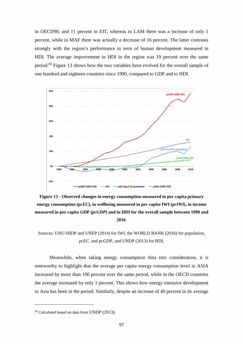
97

in OECD90, and 11 percent in EIT, whereas in LAM there was a increase of only 1

percent, while in MAF there was actually a decrease of 16 percent. The latter contrasts

strongly with the region’s performance in term of human development measured in

HDI. The average improvement in HDI in the region was 19 percent over the same

period.89 Figure 13 shows how the two variables have evolved for the overall sample of

one hundred and eighteen countries since 1990, compared to GDP and to HDI.

Figure 13 - Observed changes in energy consumption measured in per capita primary

energy consumption (pcEC), in wellbeing measured in per capita IWI (pcIWI), in income

measured in per capita GDP (pcGDP) and in HDI for the overall sample between 1990 and

2010.

Sources: UNU-IHDP and UNEP (2014) for IWI, the WORLD BANK (2016) for population,

pcEC, and pcGDP, and UNDP (2013) for HDI.

Meanwhile, when taking energy consumption data into consideration, it is

noteworthy to highlight that the average per capita energy consumption level in ASIA

increased by more than 100 percent over the same period, while in the OECD countries

the average increased by only 1 percent. This shows how energy intensive development

in Asia has been in the period. Similarly, despite an increase of 40 percent in its average

89 Calculated based on data from UNDP (2013).

98

per capita energy consumption, MAF was not able to see any improvement in its

wellbeing.

4.3. Projecting aggregate levels of human wellbeing into 2050

Next, we project the aggregate levels of human wellbeing measured in per capita

IWI (pcIWI) forward to 2030 and 2050 based on rates of change in human wellbeing

over time (r) and estimated population growth (projectedPop) from the IAM

MESSAGE (v.4) used in the LIMITS project (KRIEGLER et al., 2013, TAVONI et al.,

2013 and 2014), as follows:

Three sets of growth rates (r) were used for each region. The average compound

annual growth rate between 2005 and 2010 was used to project increases in well-being

for the years 2011 through 2020. The average between 2000 and 2010 was used for the

years 2021 through 2030. And the average between the whole observed time period

(1990-2010) was used for the remaining years. Projected population levels were

calibrated to the start of the projection period.

All data from the IAM MESSAGE v.4 were obtained from the LIMITS Scenario

Database (LIMITS Database, 2016) and confirmed in IPCC’s AR5 Scenario Database

(IAMC AR5 Scenario Database, 2014). Projected levels of wellbeing across all regions

for years 2030 and 2050 are shown in Table 3.

99

Table 3 - Per capita IWI across all RC5 regions in 2010 and projected to 2030 and 2050.

pcIWI

(in 2005 US$)

ALL

REGIONS ASIA EIT LAM MAF OECD-90

pop weighted ave. in 2010 92,602 20,779 104,831 75,944 41,956 405,396

median 72,736 17,749 95,038 69,748 31,930 433,946

min 4,627 5,596 4,627 5,627 5,721 75,600

max 758,631 269,065 247,078 139,499 533,044 758,631

pop weighted ave in 2030 31,820 117,308 88,282 42,705

change 2010-2030 53% 12% 16% 2%

pop weighted ave in 2050 49,861 133,316 113,558 44,406

change 2010-2050 140% 27% 50% 6%

Note: IPCC’s RC5 regions: Asia (ASIA) - most Asian countries with the exception of the Middle East, Japan and Former Soviet Union states, Economies in Transition (EIT) – countries from the Reforming Economies of Eastern Europe and the Former Soviet Union, Latin America (LAM) - countries of Latin America and the Caribbean, Middle East and Africa (MAF) - countries of the Middle East and Africa, and OECD 90 countries (OECD90) - countries that were members of the Organization for Economic Co-operation and Development (OECD) in 1990. See Appendix D for list of countries.

ASIA and MAF represent the regions with the greatest need for improvement in

collective wellbeing, based on their per capita IWI (pcIWI) levels. However, our

projections indicate that, of the two, only ASIA is on track to achieve significantly

higher levels of collective wellbeing by mid-century. This is primarily explained by the

fact that, assuming a continuation of the past trend observed, produced capital gains

would not only offset all natural capital losses in this region but also allow for a

substantial increase in IWI. Meanwhile, MAF would continue to see much shallower

growth rates in produced capital and continued losses in natural capital, leading to small

improvements in overall wellbeing in this region.

Conversely, LAM and EIT enjoy much higher average per capita IWI (pcIWI)

levels. However, there are countries in these regions that still bear levels equivalent to

the overall minimum, indicating that there is room for relevant improvement in their

levels of wellbeing. By contrast, with very high per capita IWI levels and a minimum

per capita IWI exceeding the median for all the selected countries in 2010, the OECD90

is not perceived as an area where relevant improvements in wellbeing are needed, and

therefore it is not included in the analysis.

Historical and projected per capita IWI and GDP data are plotted alongside to

100

illustrate how wellbeing measured in terms of per capita IWI compares to economic

growth in each region (Figure 14). Notably, per capita IWI has grown at much lower

rates than per capita GDP in all four regions. This is expected given the changes in the

three capital components of IWI, namely natural, human, and produced capital (see

section 3.4.2). There was an overall 30 percent decline in natural capital between 1992

and 2010, compared to 56 percent and 8 percent increase in produced and human

capital, respectively (UNU-IHDP and UNEP, 2014; p.27).

Note: Observed trends (darker lines) based on historical data from 1990 to 2010 from UNU-IHDP and UNEP (2014) for IWI and from WORLD BANK (2016) for population and GDP. Per capita IWI projections from 2011 onwards (faded lines) are based on extrapolation of IWI growth in the period 1990-2010 in each region and projected population growth from the no-policy baseline scenario of the IAM MESSAGE. Per capita GDP projections (faded lines) are based on estimated growth rates of GDP (PPP) and population from the IAM MESSAGE v.4. Horizontal dashed line refers to the 2010 overall population weighted average pcIWI for all one hundred and eighteen countries covered. OECD-1990 countries had over $400,000 pcIWI in 2010 (not shown on graph due to scale).

Figure 14 - Observed trends and projections (faded lines) of human wellbeing measured in

per capita IWI (pcIWI) contrasted with observed trends and projections (faded lines) of

per capita GDP (pcGDP).

In MAF alone, natural capital reduced over 40 percent compared to growth rates

around 10 percent in produced capital and human capital during the same period. By

contrast, loss in natural capital (30 percent) was more than offset by increases in

produced capital and human capital in ASIA (about 120 and close to 20 percent,

101

respectively). It should be noted, however, that because the IWI framework is based on

a production perspective (production-based accounting of natural resource depletion), a

region’s IWI could be understating or overstating the value of resources required

domestically based on resources flow in international trade interactions.90

4.4. Correlating human wellbeing and energy consumption

In order to estimate the additional energy consumption levels associated with the

projected levels of wellbeing, we examine how the latter has responded to changes in

the former during the observed time period. As such, the relationship between human

wellbeing and energy consumption is examined.

Unlike previous studies discussed in section 2.4.2 above, where HDI (or

components of it) is used as an indicator of wellbeing and analyzed against energy

consumption (or emissions) data, no saturation effect is observed between the two

variables. As shown in Figure 15, the relationship between human wellbeing in terms

of per capita IWI (pcIWI) appears to scale continuously with energy consumption

measured in per capita primary energy consumption (pcEC) derived from population-

weighted energy use data from the World Development Indicators.91 92

90 The proponents of the IWI have provided a valuation analysis of natural assets in international trade that provide relevant insights into identifying the drivers of natural capital change and where there could be over- or understatements of the value of resources actually needed by domestic (open) economies for which the IWI was calculated. While resources tend to flow from poor to rich countries, there is no steadfast rule regarding the relationship between income and production or consumption driven depletions (UNU-IHDP AND UNEP, 2012). As such, even though, in general, production entails greater resource depletion than consumption in lower-income, resource-rich economies, it is not exclusively the case (e.g. India, Nicaragua, and Eastern Europe) (UNU-IHDP AND UNEP, 2012). 91 Energy use refers to use of primary energy before transformation to other end-use fuels, which is equal to indigenous production plus imports and stock changes, minus exports and fuels supplied to ships and aircraft engaged in international transport (WORLD BANK, 2016). As such, EC refers to primary energy throughout the paper. By using primary energy consumption it will be possible to measure the emission intensities associated with the overall energy supply from primary sources, as opposed to that from final consumers only, whereby energy industries (e.g. the power sector) and non-energy uses are excluded. Moreover, this will allow projected energy consumption rates to be tracked and compared with those associated with minimum quality of life referred to in the literature, in particular SPRENG (2005) and SMIL (2010). 92 EC = EU converted from koe into GJ: 1 GJ = 1 koe / 1000 x 41.868

102

Figure 15 - Correlation between human wellbeing measured in per capita IWI and energy

consumption measured in per capita primary energy over the one hundred and eighteen

countries covered here for the year 2000 (shown in log-log space).

Source: Prepared by the author using data from UNU-IHDP and UNEP (2014) and WORLD

BANK (2016).

As such, a similar approach to that of LAMB AND RAO (2015) is used to

mathematically describe the relationship between these two variables.93 After testing a

few different models for goodness of fit, the linear model in log-log form proves to be

the best model to describe this relationship and is applied to each of the one hundred

and eighteen countries, i, as follows:

Equation [1]

The log transformation generates the desired linearity in parameters. After

estimating the log-log model, the coefficient b yields the elasticity of the dependent

variable pcIWI with respect to the independent variable pcEC. In other words, it

93 The approach used in this study differs from that in LAMB AND RAO (2015) in that it uses a single indicator of human wellbeing that comprises all three dimensions of sustainable development, instead of three different ones that reflect two dimensions of sustainable development (the environment is not taken into account). Also, the energy consumption data used in this study refer to primary energy, as opposed to final energy, which was used in LAMB AND RAO (2015). Another distinction refers to the regional aggregation used. LAMB AND RAO (2015) applied the data to only three specific sub-regions - Centrally Planned Asia, South Asia, and Africa -, while this study encompassed four broader regions where improvements in wellbeing are still needed.

103

measures the estimated percent change in the dependent variable for a percent change

in the independent variable. The coefficients obtained for the years 1990, 1995, 2000,

2005, and 2010 are shown in Table 4. They reveal an increase in the elasticity of human

wellbeing over time, suggesting an overall decoupling trend for the overall sample of

countries. In other words, achieving human wellbeing is becoming steadily more

efficient, in line with the findings in STEINBERGER AND ROBERTS (2010).

Table 4 - Regression results from Equation [1].

R-square

n % world pop

a b p-value of b

1990 0.64 118 93 7.19 0.98 0.000

1995 0.77 118 93 6.73 1.09 0.000

2000 0.79 118 93 6.56 1.13 0.000

2005 0.78 118 93 6.46 1.13 0.000

2010 0.78 118 93 6.34 1.15 0.000 Note: n = number of countries. Data for the following countries are available from 1991, thus all data refer to 1991 instead of 1990: Croatia, Kazakhstan, Kyrgyzstan, Lithuania, Russian, Federation, Slovenia, Tajikistan, and Ukraine. Data for the following countries are available from 1992, thus all data refer to 1992 instead of 1990: Czech Republic, Slovakia.

For IWI, this decoupling means that the positive impacts of increased energy

consumption on the different capitals that comprise the indicator have increasingly

outweighed the negative impacts on them between 1990 and 2010. Energy consumption

can lead to, or be associated with, increases in produced capital (e.g. investments in

infrastructure) (UNU-IHDP and UNEP, 2014). Several studies on the relationship

between energy consumption and GDP have found causality running from energy

consumption to GDP in several countries (CHEN et al., 2012; OZTURK, 2010),

described as the growth hypothesis discussed in section 2.4.1. Increased energy

consumption can also promote higher educational levels, as a result of greater access to

electricity (e.g. increased hours and flexibility for studying, greater numbers of schools),

and thereby increases in human capital (UNU-IHDP and UNEP, 2014).94

94 Based on preliminary analyses, the IWR 2014 report (UNU-IHDP and UNEP, 2014) indicates that an increase of 1 percent in energy consumption is associated with a positive variation of 0.64 percent in produced capital and 0.4 percent in human capital.

104

Conversely, because energy needs have been primarily met through depletion of

fossil-fuel deposits,95 energy consumption has a direct negative impact on IWI’s natural

capital component. However, these negative impacts have subsided gradually as

economies have been transitioning to more efficient and cleaner energy matrices, and

thereby reducing their reliance on fossil fuels, albeit at different paces.96

We then examine the same relationship in each RC5 region, except in OECD90.

As noted in section 4.3, the latter is not perceived as a region where relevant

improvements in wellbeing are needed. Notably, the linear model in log-log form

continues to fit well in the four regions where improvements in collective wellbeing are

still needed, as depicted in Figure 16.

Note: A total of eighty-eight countries were assessed (sixteen in ASIA, twenty-one in EIT, nineteen in LAM, and thirty-two in MAF) after six outliers were removed, as follows: one from EIT, three from LAM, and two from MAF.

Figure 16 - Correlations of human wellbeing measured in per capita IWI (pcIWI) and

energy consumption measured in per capita energy consumption (pcEC) in log-log form

across four of the RC5 regions in the year 2010.

Source: Prepared by the author based on data from UNU-IHDP and UNEP (2014) and WORLD

BANK (2016). 95 Fossil fuels (oil, coal, and gas) account for 85 percent of total primary energy supplies (BP, 2016). 96 The contribution of renewable energy sources to the global energy mix has been growing over the last two decades, particularly in the electricity sector (IRENA, 2016).

105

On the other hand, the decoupling trend does not prove consistent in all regions.

ASIA has mostly seen decreasing elasticities overtime and MAF has not seen much

variation, as depicted in Figure 17. This suggests that the negative impacts of increased

energy consumption on IWI’s natural capital have increasingly outweighed and offset

its positive impacts on IWI’s produced and human capitals in ASIA and MAF,

respectively. This is in part a result of large deployment of fossil fuels, which have

prevailed in particular in ASIA’s energy mix (BP, 2016).97 Meanwhile for MAF, the

negative impacts on IWI’s natural capital seem to have been mostly compensated by the

positive ones on the other two capitals, on a per capita basis. This is likely due to

continued high share of fossil fuels in the energy mix of the region (WORLD BANK,

2017), as well as, a result of the higher than average population growth rate seen in this

region during this period (UNU-IHDP and UNEP, 2014).

Note: Sixteen countries were assessed in ASIA, twenty-one in EIT, nineteen in LAM, and thirty-two in MAF, after six outliers were removed, as follows: one from EIT, three from LAM, and two from MAF. The dashed line refers to the elasticities obtained in the assessment of all one hundred and eighteen countries (see Table 4). Key: An elasticity of 1.20 means that for each 1 percent change in energy consumption (pcEC), there was a 1.20 percent change in wellbeing (pcIWI).

Figure 17 - Change in elasticity (b values) over time.

97 Exceptionally between 1995 and 2000, the energy elasticity of well-being increased in Asia, as depicted in Figure 17. This can be explained by the temporary decline in coal consumption seen in this period, believed to have been caused by a combination of the following factors: a general economic slowdown that resulted from the Asian crisis, higher coal quality, systematic closures of inefficient state-owned facilities, a general increase in end-use efficiency, as well as some substitution of coal for gas (SINTON AND FRIDLEY, 2000).

106

4.5. Estimating the additional energy needed and associated carbon emissions

The fit parameters obtained through the regression runs obtained in Section 4.4

could be linearly projected to generate future elasticities, which could in turn be used to

estimate the additional energy consumption associated with future improvements in

human wellbeing in each of the selected four regions. By doing so, specific aspects

affecting the relationship between energy consumption and IWI in each region would be

taken into consideration. For instance, natural capital is directly impacted by energy

consumption, however its share in the IWI composition varied from 8 to 40 percent in

average in the period from 1990 to 2010 depending on the region.98

However, by doing so, the analysis could be distorted by unique systemic events

that are unlikely to repeat in the future and would not take into consideration different

possibilities throughout the forecast period. Therefore, a sensitivity range is devised for

each region instead, using the highest observed decrease rate in elasticity (coefficient b)

to progressively decrease elasticities from 2011 to 2020 and maintaining it constant

thereafter as the upper bound, and the highest observed increase rate in elasticity to

progressively increase elasticities from 2011 to 2020 and maintaining it constant

thereafter as the lower bound (see Table 5). Thereby, regional differences are still taken

into consideration while allowing for annual fluctuations in future elasticities.

Table 5 - Compound annual rates of change (%) in elasticity.

ASIA EIT LAM MAF 1990-1995 -1.266 3.193 -0.455

1995-2000 0.713 3.646 -1.257 0.181

2000-2005 -0.798 0.675 1.079 -0.343

2005-2010 -0.499 -0.781 0.150 0.184

Upper bound

2011-2020 -0.635 -0.391 -0.631 -0.228 Lower bound

2011-2020 0.356 0.337 0.538 0.092 Notes: No elasticity change calculated for 1990-1995 in EIT since the

98 Calculated based on natural capital data from UNU-IHDP and UNEP (2014).

107

linear model did not fit well for the 1990 data. Positive change denotes

decoupling trend between energy consumption (pcEC) and wellbeing

(pcIWI). Upper bound rates calculated based on prorated highest decrease

rates observed, applied in the 10-year period 2011-2020. Lower bound

rates calculated based on prorated highest increase rates observed, applied

in the 10-year period 2011-2020. Second highest rates used to avoid

distortions from peaks in EIT and LAM.

By applying equation 1 and the two levels of change in elasticity (lower and

upper bounds in Table 5) to annually projected pcIWI (in 2005US$) for each region, j

(see section 4.3), the estimated lower and upper bounds of the range of projected per

capita primary energy consumption (projected pcEC) are obtained for each year after

2010, as follows:

Equation [2]

The projected pcEC for each region, j, for the years 2011 through 2050 are then

calibrated to the historical primary energy consumption data by applying their growth

rates starting with the last observed value of pcEC, i.e. in 2010, which was obtained

from a population-weighted energy use data from the World Development Indicators

(WORLD BANK, 2016). By doing this, we adjust the projections to likely differences

in data sources, regional boundaries and other assumptions used in the IAM MESSAGE

v.4 projections, following the same approach taken by LAMB AND RAO (2015).

The normalized values of the projected pcEC (Nprojected pcEC) are then scaled

by population to derive overall annual primary energy consumption levels (projected

EC) for each region, j, using normalized population projections from the IAM

MESSAGE (NprojectedPOP),99 as follows:

Equation [3]

99 As noted in section 4, all IAM MESSAGE data were obtained from the LIMITS Scenario Database (LIMITS Database, 2016) and confirmed in IPCC’s AR5 Scenario Database (IAMC AR5 Scenario Database, 2014).

108

Subsequently, the associated carbon emissions (projected CO2 emissions) are

estimated for each region, j, by applying normalized CO2 emission intensities

projections from the same no-policy baseline scenario of the IAM MESSAGE (IAMC

AR5 Scenario Database, 2014; LIMITS Database, 2016) to the projected EC, as

follows:

Equation [4]

The normalized projected CO2 emission intensities (Nprojected CO2 emission

intensities) are calculated based on projected CO2 emissions from fossil fuel combustion

and industrial processes and primary energy data from the no-policy baseline scenario

of the IAM MESSAGE v.4 (IAMC AR5 Scenario Database, 2014; LIMITS Database,

2016),100 normalized to that of 2010 based on four sets of growth rates for each region,

as shown in Table 6.

Table 6 - Compound annual rates of change (%) in CO2 emission intensity.

ASIA EIT LAM MAF

2011-2020 0.31 -0.04 0.61 0.18

2021-2030 0.19 0.15 0.03 -0.13

2031-2040 0.14 0.07 0.51 -0.07

2041-2050 0.00 0.04 -0.41 0.05

Source: own calculations based on projected CO2 emissions from fossil fuel

combustion and industrial processes and primary energy consumption data

from LIMITS Database (2016) and IAMC AR5 Scenario Database (2014).

Following the calculations above, the lower and upper bounds of projected CO2

emissions for each of the four regions are obtained for each year of the projection

period, i.e. from 2011 to 2050. 100 The Scenario Base (or no-policy baseline) in the LIMITS project refers to the standard no climate policy baseline run, which reflects development and emissions pathways unconstrained by mitigation actions (KRIEGER et al., 2013, TAVONI et al., 2014).

109

5. Results

Results of the quantitative assessment described above are presented in this

chapter. The estimated CO2 emissions required for higher levels of collective wellbeing

are then compared with regional emissions pathways based on two stabilization

scenarios from the same integrated assessment model used in the quantitative

assessment (the IAM MESSAGE used in the LIMITS project) (section 5.2).

These two stabilization scenarios provide the two carbon budgets, against which

estimated additional carbon emissions (projected CO2 emissions) associated with future

improvements in human wellbeing assuming different climate policy scenarios are

compared to (section 5.3).

5.1. Additional energy needed and associated emissions

Table 7 presents the estimated additional primary energy consumption

(projected EC) and the associated carbon emissions (projected CO2 emissions) resulting

from the projected future improvements in human wellbeing in each of the four selected

regions by 2030 and 2050.

Table 7 - Annual results from Equations [3] and [4].

n % world pop

Projected EC (EJ/year)

Projected CO2 emissions (GtCO2/year)

By 2030 By 2050 By 2030 By 2050 lower upper lower upper lower upper lower upper

ASIA 16 52 265 393 418 645 19.5 28.9 31.3 48.2

MAF 32 13 71 80 95 108 4.0 4.6 5.4 6.1

LAM 19 8 35 57 45 75 1.9 3.1 2.5 4.1

EIT 21 5 46 66 48 69 2.8 4.0 3.0 4.3

Total 88 78 417 596 606 897 28.3 40.7 42.1 62.8 Notes: n = number of countries (6 outliers removed: 2 from MAF, 3 from LAM, 1 from EIT). Projected EC = estimated additional primary energy consumption in Exajoule (EJ).

Overall, the four regions combined would require between 417 and 596 EJ in

primary annual energy consumption and between 28.3 and 40.7 GtCO2 in annual carbon

110

emissions by 2030 to increase current levels of wellbeing and between 606 and 897 EJ

and between 42.1 and 62.8 GtCO2 by 2050 to improve it even further. Their cumulative

values are presented in table 8.

Table 8 - Cumulative results from Equations [3] and [4].

n % world pop

Projected EC (EJ)

Projected CO2 emissions (GtCO2)

2011-2030 2011-2050 2011-2030 2011-2050 lower upper lower upper lower upper lower upper

ASIA 16 52 4,293 5,859 11,088 16,154 285 424 817 1,192

MAF 32 13 1,200 1,3289 2,859 3,214 63 76 162 183

LAM 19 8 644 942 1,444 2,267 31 51 80 125

EIT 21 5 933 1,225 1,874 2,581 51 75 115 158

Total 88 78 7,070 9,366 17,264 24,216 430 626 1,174 1,658

Notes: n = number of countries (6 outliers removed: 2 from MAF, 3 from LAM, 1 from EIT). Projected EC = estimated additional primary energy consumption in Exajoule (EJ).

In terms of cumulative values the four regions combined would require between

7,070 and 9,366 EJ in overall primary energy consumption and between 430 and 626

GtCO2 in overall carbon emissions from 2011 to 2030 and between 17,263 and 23,871

EJ and between 1,174 and 1,658 GtCO2 from 2011 to 2050 to achieve higher

collective wellbeing. Ultimately, cumulative emissions are what matters most in terms

of meeting the climate stabilization targets (MEINSHAUSEN et al., 2009; KRIEGLER

et al., 2013; KNUTTI AND ROGELJ, 2015; ROGELJ et al., 2016b).

A comparison with previous quantification efforts in the literature that used HDI

or components of it as proxy for human wellbeing is provided in Appendix E. The

energy levels estimated in the present study are at least 23 percent higher than previous

quantifications found in the literature (PASTERNAK, 2000; UGURSAL, 2014) and the

CO2 emissions estimates are at least 38 percent higher than previous quantifications

(COSTA et al., 2011; LAMB AND RAO, 2015).

5.1.1. In ASIA

Representing by far the largest region in terms of population, ASIA alone would

111

account for approximately 61 to 67 percent of the estimated additional primary energy

consumption needed and 66 to 72 percent of the associated carbon emissions.

According to the results obtained, achieving increased levels of human

wellbeing in ASIA would entail between 265 and 393 EJ (63-94 GJ/capita) in primary

annual energy consumption and between 19.5 and 28.9 GtCO2 in annual carbon

emissions by 2030, and 418-645 EJ (94-146 GJ/capita) and between 31.3 and 48.2

GtCO2 by 2050. In terms of cumulative energy consumption and carbon emissions, the

projected pathways for this region indicate a total of at least 4,293 EJ and 285 GtCO2 in

the 2011-2030 period, and 11,088 EJ and 817 GtCO2 in 2011-2050. These levels are

associated with an increase of 53 percent in wellbeing in per capita IWI (pcIWI)

between 2010 and 2030 and 140 percent between 2010 and 2050 (see Table 4 in section

4.3).

Even though the absolute values of pcIWI cannot provide a direct indication of

whether ASIA would achieve a sufficiently high level of wellbeing, the scale of its

relative change (53 percent) and the average primary energy consumption rate reached

already in 2030 point to a significant achievement. According to the projections

obtained in this analysis, the primary energy consumption rate in ASIA is expected to

increase from 49 to at least 63 and up to 94 GJ/capita between 2010 and 2030, thus

likely moving out of the energy poverty levels discussed in section 2.2 before mid-

century.

5.1.2. In the Middle East and Africa (MAF)

The second largest region, MAF, representing 13 percent of the world

population, would require between 71 and 80 EJ (53-61 GJ/capita) in primary annual

energy consumption and between 4.0 and 4.6 GtCO2 in annual carbon emissions by

2030 to practically sustain current levels of wellbeing in pcIWI. It would then require

between 95 and 108 EJ (55-63 GJ/capita) and between 5.4 and 6.1 GtCO2 by 2050 to

improve wellbeing by 6 percent (see Table 4 in section 4.3). In terms of cumulative

energy consumption and carbon emissions, the projected pathways for MAF indicate a

total of at least 1,200 EJ and 63 GtCO2 in the 2011-2030 period, and 2,859 EJ and 162

GtCO2 in 2011-2050.

112

Unlike ASIA, MAF is unlikely to move out of the energy poverty levels

discussed in section 2.2 between 2010 and 2030 since its average primary energy

consumption rate would increase from 54 to up to 61 GJ/capita in the same period

according to the projections obtained in this analysis. In fact, not even the projections

into 2050 indicate any likelihood of the region moving much further out of the energy

poverty levels. Its primary energy consumption rate would increase to up to 63

GJ/capita by 2050.

5.1.3. In Latin America (LAM)

LAM follows next in population size, accounting for 8 percent of the world

population. Achieving a 16 percent increase in wellbeing by 2030 in this region would

entail between 35 and 57 EJ (51-83 GJ/capita) in average primary annual energy

consumption and between 2.4 and 3.1 GtCO2 in annual carbon emissions by the same

year. Similarly, achieving a 50 percent increase by mid-century would entail between

45 and 75 EJ (61-103 GJ/capita) in average primary annual energy consumption and

between 2.5 and 4.1 GtCO2 by then. In terms of cumulative energy consumption and

carbon emissions, the projected pathways for this region indicate a total of at least 644

EJ and 31 GtCO2 in the 2011-2030 period, and 1,444 EJ and 80 GtCO2 in 2011-2050.

According to the projections obtained in this analysis, the expected range of

increase from 56 to up to 83 GJ/capita between 2010 and 2030 indicates that, similar to

ASIA, LAM is also likely to move out of the energy poverty levels discussed in section

2.2 before mid-century.

5.1.4. In Economies in Transition (EIT)

The fourth and last region assessed, representing only 5 percent of the world

population, EIT would require between 46 and 66 EJ (139-199 GJ/capita) in average

primary annual energy consumption and imply in annual carbon emissions between 2.8

and 4.0 GtCO2 by 2030 to increase current levels of wellbeing by 12 percent, and

between 48 and 69 EJ (154-222 GJ/capita) and 3.0 and 4.3 GtCO2 by 2050 to improve it

by 27 percent. In terms of cumulative energy consumption and carbon emissions, the

113

projected pathways for EIT indicate a total of at least 933 EJ and 51 GtCO2 in the 2011-

2030 period, and 1,874 EJ and 115 GtCO2 in 2011-2050, as shown in Figure 18b.

Clearly, this region not only already enjoys the highest levels of wellbeing

among the four regions under analysis in both absolute per capita IWI terms, as well as,

in terms of energy consumption rates, but is also set to improve them even further.

5.2. Wellbeing versus climate stabilization: comparing emissions pathways

The calculations used to estimate the CO2 emissions associated with bridging

the energy divide and achieving higher collective wellbeing assumed CO2 emission

intensities based on data from the no-policy baseline scenario of the IAM MESSAGE

v.4. This scenario refers to the standard no climate policy and target baseline run of the

model. It reflects no new climate policy or mitigation action beyond what has already

been put in place (as of 2010). As such, the results of equation 4 (projected CO2

emissions) provided in sections 5.1 and 5.2 refers to a No-action scenario, and thus

reflect prevailing technologies and decarbonisation rates.

5.2.1. Associated emissions under no-action scenario

In order to determine whether the estimated carbon emissions needed to achieve

higher levels of collective wellbeing would affect existing carbon budgets, their

emission pathways were compared with regional emissions pathways associated with

the 2 oC climate stabilization target. Notably, over one hundred climate policy scenarios

have been produced in the literature based on different probabilities of reaching this

target (CLARKE et al., 2014, Kriegler et al., 2014b), as discussed in section 2.3.2. In

fact, there are many different emissions pathways and timings associated with meeting

different intended climate stabilization targets (ROGELJ et al., 2011, 2015 and 2016b;

CLARKE et al., 2014; DESSENS et al., 2014; UNEP, 2015).101

For this assessment, two stabilization scenarios from the same IAM used in the

101 Emissions profiles in the existing modeling literature are determined by three interrelated factors: (1) the degree of overshoot, (2) technology options and associated deployment decisions, and (3) policy assumptions (CLARKE et al., 2014).

114

quantitative analysis above (the IAM MESSAGE used in the LIMITS project) were

used (IAMC AR5 Scenario Database, 2014; LIMITS Database, 2016), namely: Scenario

450 and Scenario 500, which are associated with reasonably high and even chances of

meeting the 2 oC climate stabilization target, respectively (TAVONI et al., 2014). These

two stabilization scenarios are hereinafter referred to as Immediate action-450 and

Immediate action-500, respectively.

These two stabilization scenarios provide the two carbon budgets used in this

assessment, i.e. the 450-ppm and 500-ppm budgets. In both scenarios, even though

energy consumption is set to increase, CO2 emissions would fall below the levels that

our assessment indicated would be required to achieve and sustain higher collective

wellbeing in all four regions by mid-century (Figure 18). This is most noticeable in

ASIA, where the estimated gap could range from 23 to 43 GtCO2 by mid-century and is

much higher than the range of 7 to 12 GtCO2 estimated for the other three regions

combined.

115

Figure 18 - Estimated annual primary energy and CO2 emissions pathways for achieving

higher levels of human wellbeing in ASIA, EIT, LAM, and MAF, compared to two

stabilization scenarios from the IAM MESSAGE (Immediate action-450 and Immediate

action-500), which would yield reasonably high and even chances of achieving 2oC,

respectively.

Sources: own calculations following the quantitative assessment presented in section 4.5 and

IAMC AR5 Scenario Database (2014) and LIMITS Database (2016) for policy scenarios.

116

In both climate policy scenarios, cumulative emissions fall short of the estimated

amounts required for achieving higher levels of collective wellbeing, primarily in ASIA,

where the gap could be at least 26 GtCO2 and as high as 231 GtCO2 between 2011 and

2030 (Figure 19a) and at least 291 GtCO2 and as high as 771 GtCO2 between 2011 and

2050 (Figure 19b). By contrast, the largest gaps in the other three regions combined

would not exceed about 95 GtCO2 in the first period and about 232 GtCO2 in the second

one.

Note: The shaded bars refer to the upper (darker tone) and lower (lighter tone) bounds of the sensitivity range of the projection.

Figure 19 - Estimated cumulative primary energy and CO2 emissions for achieving higher

levels of human wellbeing in ASIA, EIT, LAM, and MAF in 2011-2030 and 2011-2050,

compared to two standard benchmark policy scenarios from the IAM MESSAGE v.4

(Immediate action-450 and Immediate action-500), which are associated with reasonably

high and even chances of meeting the 2 oC target, respectively.



117

As discussed in section 4.3 above, with population-weighted averages of per

capita IWI expected for 2050 still close to half of the overall average from 2010, ASIA

and MAF are the regions with the greatest need for improvement in collective

wellbeing. However, based on the projections obtained here, of the two, only ASIA

would be able to achieve substantial improvements in the period under analysis,

primarily due to the fact that, assuming a continuation of the past trend observed,

produced capital gains would not only offset all natural capital losses in this region but

also allow for a substantial increase in IWI. Hence, the expected 53 percent increase in

per capita IWI in the region already by 2030.

Meanwhile, given much shallower growth rates in produced capital and

continued losses in natural capital, overall per capita IWI in MAF is only expected to

see mere 2 percent and 6 percent increases by 2030 and 2050, respectively. This

explains the expected small gap ranges between cumulative emissions in the two policy

scenarios and those required to achieve higher levels of collective wellbeing in this

region of at least 5 and up to 30 GtCO2 in the first period (2011 to 2030) and at least 35

and up to 71 GtCO2 in the second one (2011 to 2050).

In any case, in spite of MAF’s expected inability to achieve a significantly high

level of human wellbeing by mid-century, the small improvements projected for this

region could exceed the emissions budget for the region by over 60 percent, i.e. 183

GtCO2 in the upper bound projection from this analysis compared to 112 GtCO2 in the

most stringent of the two climate policy scenarios (Immediate action-450).

Considering all four regions combined and the emission pathways of the two

IAM MESSAGE stabilization scenarios associated with reasonably high and even

chances of limiting the temperature increase to below 2 oC, Immediate action-450 and

Immediate action-500, the corresponding overall carbon budgets could be exceeded by

as much as two and a half times (1,003 GtCO2) and about two times (856 GtCO2) by

mid-century, respectively.

118

5.2.2. Climate action scenarios

In order to help us determine what can be done to bridge the energy divide and

achieve higher levels of wellbeing while staying within the carbon budget, we looked at

three alternative scenarios from the IAM MESSAGE v.4, wherein new climate policy

and actions are considered to project future CO2 emissions associated with higher

collective wellbeing, namely: Action as of 2020-500 (RefPol-500 in the LIMITS

project), Action as of 2020-450 (RefPol-450 in the LIMITS project), and Delayed

action-500 (RefPol2030-500 in the LIMITS project). These three climate policy

scenarios are discussed in the next sections. All six scenarios used in this analysis are

summarized in Table 9.

Table 9 - Emissions scenarios.

Scenario name Corresponding

scenario in

LIMITS study

Scenario

type

Fragmente

d action

until

Long-term

target (2100)

No-action Base Baseline n/a none

Immediate action-500 500 Stabilization n/a 500 ppm CO2eq

(3.2 W/m2)

Immediate action-450 450 Stabilization n/a 450 ppm CO2eq

(2.8 W/m2)

Action as of 2020-500 RefPol-500 Climate

policy 2020

500 ppm CO2eq

(3.2 W/m2)

Action as of 2020-450 RefPol-450 Climate

Policy 2020

450 ppm CO2eq

(2.8 W/m2)

Delayed action-500 RefPol-2030-

500

Climate

policy 2030

500 ppm CO2eq

(3.2 W/m2)

Source: Adapted from KRIEGLER et al., 2013.

5.2.3. Associated emissions under Action as of 2020-500 scenario

The Action as of 2020-500 scenario (RefPol-500 in the LIMITS project) refers

to a scenario where regions follow existing domestic policies or mitigation actions until

2020 and adopt new policies and actions associated with even chances of meeting the 2 oC target, i.e. reaching GHG concentrations at roughly 500 ppm CO2e in 2100,

119

thereafter.

New projected CO2 emission intensities (Nprojected CO2 emission intensities)

are calculated based on projected CO2 emissions from fossil fuel combustion and

industrial processes and primary energy data from the RefPol-500 of the IAM

MESSAGE v.4 (IAMC AR5 Scenario Database, 2014; LIMITS Database, 2016),

normalized to that of 2010 based on four sets of growth rates for each region, as shown

in Table 10.

Table 10 - Compound annual rates of change (%) in CO2 emission intensity

on the Action as of 2020-500.

ASIA EIT LAM MAF

2011-2020 -0.08 -0.48 -1.48 -0.06

2021-2030 -0.74 -2.06 -1.92 -2.14

2031-2040 -3.05 -3.91 -4.26 -2.85

2041-2050 -5.01 -12.25 -42.52 -6.46 Source: own calculations based on projected CO2 emissions from fossil fuel

combustion and industrial processes and primary energy consumption data from

the RefPol-500 scenario of the IAM MESSAGE v.4 (IAMC AR5 Scenario

Database, 2014; LIMITS Database, 2016).

Following the calculations in section 4.5 and applying the revised projected CO2

emission intensities for Action as of 2020-500 scenario as per above to equation 4, the

estimated CO2 emissions pathways for achieving higher levels of human wellbeing are

revised, as shown in Figure 20.

120


levels of human wellbeing in ASIA, EIT, LAM, and MAF in the Action as of 2020-500,

compared to projections based on two stabilization scenarios from the IAM MESSAGE

(Immediate action-450 and Immediate action-500), which would yield reasonably high and

even chances of achieving 2oC, respectively.


revised projected CO2 emission intensities for the Action as of 2020-500 scenario; and


121

5.2.4. Associated emissions under Action as of 2020-450 scenario

The Action as of 2020-450 scenario (RefPol-450 in the LIMITS project) refers

to a scenario where regions follow existing domestic policies or mitigation actions until

2020 and adopt new policies and actions associated with reasonably high chances of

meeting the 2 oC target, i.e. reaching GHG concentrations at roughly 450 ppm CO2e in

2100, thereafter.



industrial processes and primary energy data from the RefPol-450 of the IAM

MESSAGE v.4 (IAMC AR5 Scenario Database, 2014; LIMITS Database, 2016),


in Table 11.


on the Action as of 2020-450.

ASIA EIT LAM MAF

2011-2020 -0.08 -0.48 -1.48 0.06

2021-2030 -1.75 -3.45 -3.14 -2.88

2031-2040 -5.27 -6.50 -5.88 -4.09

2041-2050 -6.56 -17.46 -40.79 -10.70 Source: own calculations based on projected CO2 emissions from fossil fuel

combustion and industrial processes and primary energy consumption data

from the RefPol-450 scenario of the IAM MESSAGE v.4 (IAMC AR5

Scenario Database, 2014; LIMITS Database, 2016).


emission intensities as per above to equation 4, the estimated CO2 emissions pathways

for achieving higher levels of human wellbeing are revised, as shown in Figure 21.

122


levels of human wellbeing in ASIA, EIT, LAM, and MAF in the Action as of 2020-450,

compared to projections based on two stabilization scenarios from the IAM MESSAGE

(Immediate action-450 and Immediate action-500), which would yield reasonably high and

even chances of achieving 2oC, respectively.


revised projected CO2 emission intensities for Action as of 2020-450 scenario; and LIMITS

Database (2016) and IAMC AR5 Scenario Database (2014) for policy scenarios.

123

5.2.5. Associated emissions under Delayed action-500 scenario

The Delayed action-500 scenario (RefPol2030-500) refers to a scenario where

regions follow existing domestic policies or mitigation actions until 2030 and adopt new

policies and actions associated with even chances of meeting the 2 oC target, i.e.

reaching GHG concentrations at roughly 500 ppm CO2e in 2100, only thereafter.



industrial processes and primary energy data from the RefPol2030-500 scenario of the

IAM MESSAGE (IAMC AR5 Scenario Database, 2014; LIMITS Database, 2016),


in Table 12.


on the Delayed action-500 scenario.

ASIA EIT LAM MAF

2011-2020 -0.08 -0.48 -1.48 0.06

2021-2030 0.19 -0.02 -0.53 -0.21

2031-2040 -3.19 -4.18 -3.08 -2.57

2041-2050 -4.77 -11.81 -9.75 -4.27

Source: own calculations based on projected CO2 emissions from fossil fuel

combustion and industrial processes and primary energy consumption data from

the RefPol2030-500 scenario of the IAM MESSAGE (IAMC AR5 Scenario

Database, 2014; LIMITS Database, 2016).


emission intensities as per above to equation 4, the estimated CO2 emissions pathways

for achieving higher levels of human wellbeing are revised, as shown in Figure 22.

124


levels of human wellbeing in ASIA, EIT, LAM, and MAF in the Delayed action-500

scenario, compared to projections based on the stabilization scenarios from the IAM

MESSAGE (Immediate action-450 and Immediate action-500), which would yield

reasonably high and even chances of achieving 2oC, respectively.


revised projected CO2 emission intensities for the Delayed action-500 scenario; and LIMITS

Database (2016) and IAMC AR5 Scenario Database (2014) for policy scenarios.

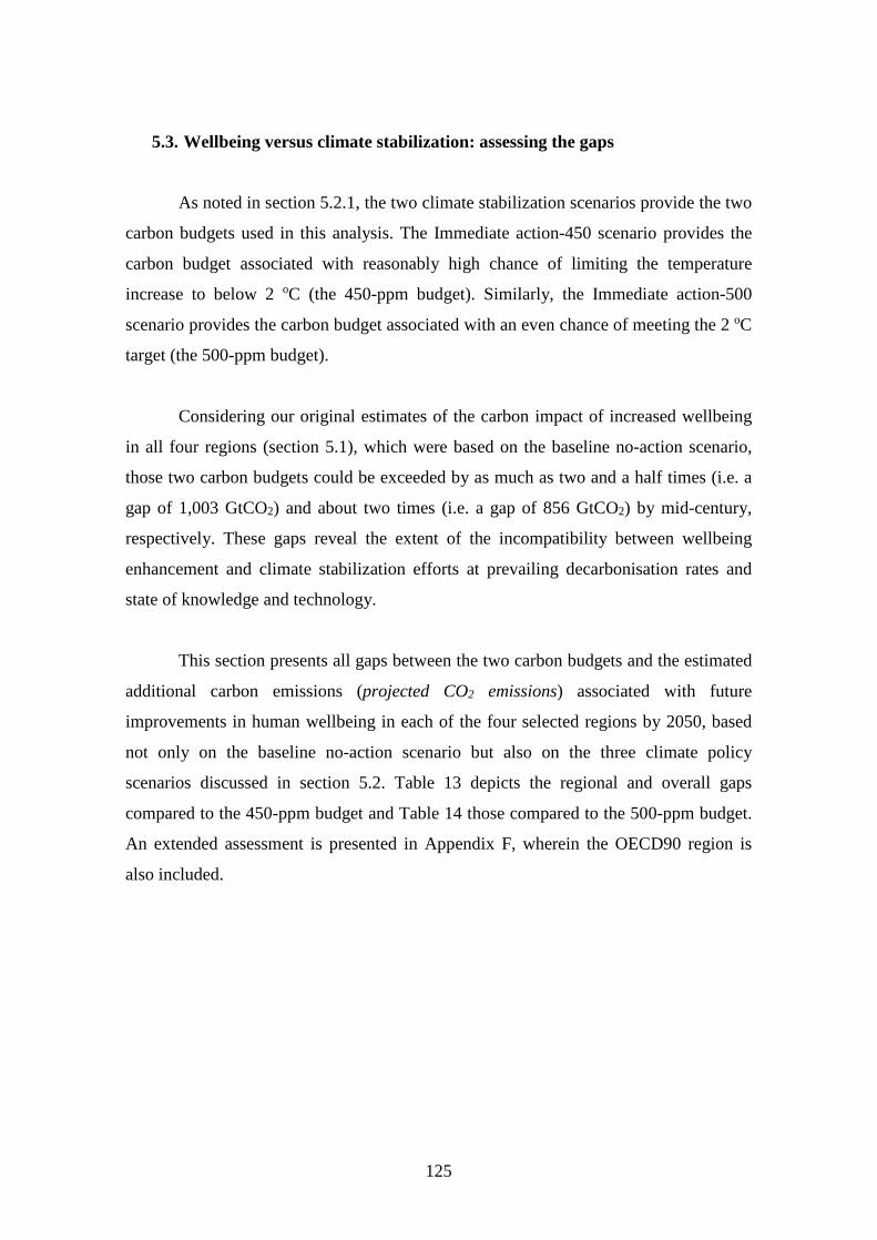
125

5.3. Wellbeing versus climate stabilization: assessing the gaps

As noted in section 5.2.1, the two climate stabilization scenarios provide the two

carbon budgets used in this analysis. The Immediate action-450 scenario provides the

carbon budget associated with reasonably high chance of limiting the temperature

increase to below 2 oC (the 450-ppm budget). Similarly, the Immediate action-500

scenario provides the carbon budget associated with an even chance of meeting the 2 oC

target (the 500-ppm budget).

Considering our original estimates of the carbon impact of increased wellbeing

in all four regions (section 5.1), which were based on the baseline no-action scenario,

those two carbon budgets could be exceeded by as much as two and a half times (i.e. a

gap of 1,003 GtCO2) and about two times (i.e. a gap of 856 GtCO2) by mid-century,

respectively. These gaps reveal the extent of the incompatibility between wellbeing

enhancement and climate stabilization efforts at prevailing decarbonisation rates and

state of knowledge and technology.

This section presents all gaps between the two carbon budgets and the estimated

additional carbon emissions (projected CO2 emissions) associated with future

improvements in human wellbeing in each of the four selected regions by 2050, based

not only on the baseline no-action scenario but also on the three climate policy

scenarios discussed in section 5.2. Table 13 depicts the regional and overall gaps

compared to the 450-ppm budget and Table 14 those compared to the 500-ppm budget.

An extended assessment is presented in Appendix F, wherein the OECD90 region is

also included.

126

Table 13 – Wellbeing emissions shortfall by 2050 per emissions scenario compared to the

450-ppm budget.

Region/ Scenario

Immediate action-450 (budget)

Gap in No-action

scenario

Gap in Delayed

action-500 scenario

Gap in Action as of

2020-500 scenario

Gap in Action as of

2020-450 scenario

at least up to at

least up to at least up to at

least up to

ASIA 421 396 771 207 484 170 429 82 296

MAF 112 51 71 23 40 4 17 (9) 3

LAM 48 32 78 6 35 (8) 13 (11) 8

EIT 75 40 83 10 40 2 29 (8) 15

Total 4 regions 655 519 1,003 245 598 168 488 54 321

Budget exceeded by (times) 2.5 1.5

Table 14 – Wellbeing emissions shortfall by 2050 per emissions scenario compared to the

500-ppm budget.

Region/ Scenario


Gap in No-action

scenario

Gap in Delayed

action-500 scenario

Gap in Action as of

2020-500 scenario

Gap in Action as of

2020-450 scenario

at least up to at


least up to

ASIA 527 291 665 101 378 64 323 (24) 190

MAF 128 35 55 7 24 (12) 1 (25) (13)

LAM 57 22 68 (4) 25 (17) 3 (21) (2)

EIT 91 24 67 (6) 24 (13) 14 (23) (0)

Total 4 regions 803 372 856 98 451 21 341 (93) 174


By analyzing the corresponding shortfalls in the alternative scenarios, we can

further assess whether higher decarbonisation rates would reduce the incompatibility

between wellbeing enhancement and climate stabilization targets in individual regions

127

where improvements are needed, as well as in all such regions combined.

In ASIA, the incompatibility would likely persist even at much deeper

decarbonisation rates, given the shortfalls seen in all three alternative scenarios

considered. Only in the lower range of the projections under the most stringent of the

climate scenarios considered, the Action as of 2020-450, and considering the less

stringent budget (500-ppm budget) could the gap be fully closed.

Conversely, in the other three regions, there could be compatibility between the

two efforts at much deeper decarbonisation rates, in particular under the most stringent

of the climate scenarios considered, the Action as of 2020-450. Moreover, there is a

very small chance that LAM and EIT could afford to delay the start of new climate

policies and actions until 2030 and still be able to increase its wellbeing without

compromising their corresponding 500-ppm budgets.

Meeting energy needs and enabling the achievement of higher well-being in all

four regions combined could prove incompatible with climate stabilization even at

higher decarbonisation rates, considering that the estimated carbon budget associated

with a reasonably high chance of limiting the temperature increase to below 2 oC (the

450-ppm budget) could still be exceeded by up to 321 Gt CO2 (Table 13). Except for,

possibly, in the lower range of the projections, under the most stringent of the climate

scenarios considered, the Action as of 2020-450, and considering the less stringent

budget (500-ppm budget) (Table 14).

128

6. Analysis of results and recommendations

The results presented above in chapter 5 indicate that even with higher

decarbonisation rates associated with the adoption of new policies and actions

associated with reasonably high chances of meeting the 2 oC target, i.e. reaching GHG

concentrations at roughly 450 ppm CO2eq in 2100, starting in 2020, emissions

associated with achieving higher levels of collective well-being in all four regions

where improvements are still needed, which represent 78 percent of the global

population, could still exceed the estimated carbon budgets associated with reasonably

high and even chances of limiting the temperature increase to below 2 oC. This impact

would be even greater for lower temperature increase levels.102

As such, this study showcases the potential incompatibility between efforts

towards bridging the energy divide while enabling the achievement of higher collective

wellbeing and those associated with climate stabilization. This is primarily the case in

ASIA, where new climate policies would likely have to be adopted before 2020 and/or

even more stringent policies and actions than those associated with reasonably high

chances of meeting the 2 oC target, i.e. of reaching GHG concentrations at roughly 450

ppm CO2eq in 2100, would be required.

In the other three regions, there could be compatibility between the two efforts if

new climate policies and actions associated with reasonably high chances of meeting

the 2 oC target, i.e. of reaching GHG concentrations at roughly 450 ppm CO2eq in 2100,

were adopted as of 2020.103 Moreover, LAM and EIT could potentially afford to delay

the start of new climate actions until 2030 and still remain within their less stringent

budgets (the 500-ppm budget) should their future energy elasticities equate to those in

the lower bound of the projections, i.e. increasing from 1.24 to at least 1.30 and from

1.23 to at least 1.26 from 2011 through 2020 and remaining constant thereafter,

respectively.

102 As noted in section 2.3.1, in the Paris Agreement signed in 2015, Parties agreed to revise the target to “well below 2 oC” and to pursue further efforts aiming at limiting temperature increase to below 1.5 oC (UNFCCC, 2015). 103 However, should MAF improve its capacity to generate greater produced capital and human capital, and thereby increase its wellbeing beyond 6 percent by mid-century, there would likely be incompatibility issues similar to those seen in ASIA.

129

Based on the results obtained, this chapter discusses them, while attempting to

provide answers to the four pressing questions presented at the beginning of this thesis

(see Introduction) and some recommendations.

6.1. Answering question number 1: how much energy consumption, and its

corresponding CO2 emissions, would be needed to bridge the energy divide

and enable the achievement of higher levels of collective wellbeing?

According to the assessment carried out, meeting the urgent energy needs while

enabling the achievement of higher levels of human wellbeing in all four regions where

improvements are still needed,104 representing 78 percent of global population (based on

2010 data), would require at least 1,174 GtCO2 and as much as 1,658 GtCO2 of

cumulative emissions between 2011 and 2050, at current decarbonisation rates and state

of knowledge and technology. This range is equivalent to annual emissions of about 30

to 43 GtCO2, which are much higher than the recent (2013) level for all four regions

combined of about 20 GtCO2 (WORLD BANK, 2017).

6.2. Answering question number 2: Would the existing carbon budgets be

affected?

The estimated cumulative emissions associated with bridging the energy divide

while enabling the achievement of higher levels of wellbeing in all four regions could

exceed the overall 450-ppm budget by up to two and a half times (i.e. a gap of 1,003

GtCO2) by 2050, assuming prevailing technologies and decarbonisation rates. Similarly,

the overall 500-ppm budget could be exceeded by up to two times (i.e. a gap of 856

GtCO2) by the same time.

The carbon impact would be even greater should lower temperature increase

levels be pursued. Given the recent adoption of the Paris Agreement, current climate

stabilization efforts are already due to be strengthened with a view to keeping global

temperature rise this century well below 2 oC above pre-industrial and potentially even 104 As noted in section 4.3, the OECD-90 region is not included in the analysis as it is not as an area where relevant improvements in wellbeing are needed.

130

below 1.5 oC, as noted in section 2.3.1. 105

6.3. Answering question number 3: If so, what part(s) of the world would be

mostly at risk?

Based on the assessment carried out, ASIA and MAF are the regions with the

greatest need for improvement in collective wellbeing in terms of per capita IWI. As

discussed in section 2.2, they also represent the areas were the so-called “energy poor”

dwell in and where most of the population growth is expected to take place by mid-

century, almost 2 billion people.

By 2050, ASIA alone is expected to represent over half of the total population,

with over 4.4 billion people, while MAF would entail just over 1 billion people. This

difference partially explains why ASIA alone accounts for over 60 percent of the

estimated additional energy needed and up to 72 percent of the associated carbon

emissions, making it by far the most critical area where efforts to reduce the carbon

impact of the necessary improvements in human wellbeing would be most needed.

The estimated carbon budgets associated with reasonably high (450-ppm) and

even (500-ppm) chances of limiting the temperature increase to below 2 oC in ASIA

could be exceeded by almost three times (i.e. a gap of 771 GtCO2) and by over two

times (i.e. a gap of 665 GtCO2), respectively, by mid-century.

6.4. Answering question number 4: what needs to be done to bridge the energy

divide and increase wellbeing while staying within existing carbon

budgets?

105 ROGELJ et al. (2015) provide estimated pathways associated with limiting average global temperature warming to below 1.5 °C by 2100.

131

Based on the findings obtained, adoption of new climate policies and mitigation

actions beyond those already in place in 2010 would be critical to be able to bridge the

energy divide while enabling the achievement of higher levels of collective wellbeing

without exceeding the existing carbon budgets associated with meeting the prescribed 2 oC target.

This applies in particular to ASIA, where, for instance, the adoption of new

policies and actions associated with reasonably high chances of meeting the 2 oC target,

i.e. reaching GHG concentrations at roughly 450 ppm CO2eq in 2100, starting in 2020,

would reduce the upper range of the gap compared to the 450-ppm budget from 771 to

296 GtCO2 and the lower range from 396 to 82 GtCO2 (Table 13). It would be a

significant reduction. However, in order to fully close the gap, either such new policies

and actions would have to be adopted before 2020 or more stringent new policies and

actions, including higher deployment levels of low-carbon, carbon dioxide removal

(CDR), and/or negative emissions technologies, would likely have to be adopted

starting in 2020.

Meanwhile, MAF, EIT and LAM would also have to adopt new policies and

actions associated with high chances of meeting the prescribed 2 oC target, i.e. reaching

GHG concentrations at roughly 450 ppm CO2eq in 2100, beyond those already in place

(as of 2010), starting in 2020, in order to ensure full mitigation of the carbon impact

associated with bridging the energy divide and achieving higher levels of collective

wellbeing.

It is worth noting that these three regions would enjoy very different

improvements in wellbeing, as discussed in section 5.1, despite having somewhat

similar carbon impacts. LAM and EIT would achieve increases of 50 and 27 percent,

respectively, with LAM moving out of energy poverty levels before mid-century and

EIT improving its already decent level of energy consumption rate even further.

Meanwhile, MAF would see an increase of only 6 percent in its level of collective

wellbeing and an increase of up to 63 GJ/capita in its average primary energy

132

consumption rate by mid-century,106 neither of which indicates that the region would be

moving much further out of the energy poverty levels.

6.5. Recommendations

Meeting future energy needs with deployment of low-carbon energy

technologies would allow higher levels of collective wellbeing measured in terms of

IWI to be reached while maintaining low associated emissions, since it could

significantly reduce the impact on natural capital, otherwise driven by fossil fuels

extraction. This approach would also help unlock MAF’s ability to reach even higher

levels of collective wellbeing since investments in clean technologies would boost

produced capital and in turn yield much higher levels of IWI. Moreover, investments in

low-carbon energy technologies would improve energy security and reduce the risk of

price fluctuations for net oil-importing countries in the region (e.g. Bahrain, Israel,

Jordan, Morocco, and South Africa), thereby alleviating the challenge of expanding

energy access (OECD/IEA, 2010) without significant conflicts with climate

stabilization efforts.

However, in order to achieve higher deployment rates of cleaner technologies in

these regions investments would have to be scaled up significantly. Even though ASIA

leads global investments in renewables with an estimated USD 161 billion in 2015

(IRENA, 2017) and MAF has been attracting increased levels of investment, having

summed USD 12 billion in 2015 (IRENA, 2017),107 these levels of investments fall

considerably short of those needed to meet climate goals (IRENA, 2016). Solar and

wind power have dominated the share of investments in these regions, as well as

globally (IRENA, 2017). While there is still significant potential for further deployment

of renewables in the power sector, an untapped potential remains for the use of

renewables for heating and cooling in buildings and industry as well as for

transportation. Together, these end-user sectors account for a large portion of global

106 As noted in section 2.2, recent studies suggest that societies typically require an annual per capita primary energy consumption rate above 50 GJ (SMIL, 2010a) or 63 GJ (SPRENG, 2005) to be able to achieve decent living standards. 107 These investments include all asset classes, including asset finance, corporate R&D, government R&D, public markets, reinvested equity, small distributed capacity and venture capital, private equity (IRENA, 2017).

133

energy use and about 60 percent of energy-related CO2 emissions (IEA, 2015b).

Yet, additional capital commitments face two important barriers in these areas:

high-perceived investment risks (e.g. political, credit, currency, and power-offtake

risks) and lack of local capacity and resources for project development (IRENA, 2017).

So as to overcome these barriers, well-structured financial frameworks alongside

tailored energy policies to local circumstances and to optimize synergies, such as

between the power and end-user sectors, should be sought out.

Moreover, the levels of deployment of low-carbon energy technologies that

would be needed to fully mitigate the carbon impact associated with increased

wellbeing, in particular in ASIA, may not be realistic in the timeframe under

consideration. While there has been an increased deployment of low-carbon energy

technologies, the transition away from the current, long-established energy systems

relying overwhelmingly on fossil fuels, or what could be called the 5th great energy

transition, following the timeline presented in section 2.1, is a process that is still

unfolding and is not expected to be completed before mid-century. According to

mainstream conceptions, the current energy transition will invariably take decades to

occur based on historical record and recent advances (FOUQUET, 2010; GRUBLER,

2012; SMIL, 2006, 2010a and 2016).108

In light of these considerations, without broader, concerted collaboration

between advanced countries and the rest of the world, it will be very hard for these

regions to transition to the low-carbon and low energy-intensive pathways that would

allow them to meet pressing energy needs and secure higher levels of human wellbeing

without harming the environment or weakening social conditions that could, otherwise,

compromise the wellbeing of their future generations. As such, in order to make the

pursuit towards higher collective wellbeing compatible with climate stabilization,

advanced countries may need to go beyond technology transfers and financial assistance

and face the burden of reducing their own emissions even further to make room for

108 SMIL (2006) outlines some of the underlying reasons for the expected timing, namely: the scale of the shift; the lower energy density of the replacement fuels; the substantially lower power density of renewable energy extraction; intermittency of renewable flows; and uneven distribution of renewable energy resources.

134

increased emissions needed to secure higher collective wellbeing in the rest of the

world.

Nevertheless, as shown in Appendix F, even if new climate policies and

mitigation actions associated with reasonably high chances of meeting the 2 oC target,

i.e. reaching GHG concentrations at roughly 450 ppm CO2eq in 2100, were adopted in

all four regions where improvements are still needed as well as in advanced countries

(OECD90 region) in 2020, emissions associated with meeting the urgent energy needs

while enabling the achievement of higher levels of collective wellbeing, could still

exceed the estimated carbon budgets associated with reasonably high and even chances

of limiting the temperature increase to below 2 oC by almost one and a half times (i.e. a

gap of 397 GtCO2) and by over one time (i.e. a gap of 198 GtCO2), respectively, by

mid-century.

Given the scale of the overall gaps, to make room for increased emissions

needed to secure higher wellbeing in the rest of the world, advanced countries would

likely need to achieve very low or even net zero CO2 emissions in key energy-

dependent sectors. Such a feat would likely require deployment of mitigation strategies

beyond those aiming to achieve carbon neutrality already in 2020. As noted in section

2.3.2, there is a range of negative emissions technologies at various stages of

development under consideration worldwide. However, concerns have been raised with

regard to the safety of betting on the use of negative emissions after mid-century to

avoid dangerous climate change (e.g. FUSS et al., 2014),109 which would make the

reliance on its use already in the short- and mid-term even more questionable. The

feasibility of large-scale negative emissions programs has yet to be proven and will

require significant technological progress (SMITH and TORN, 2013), considering that

numerous resource implications associated with the widespread implementation of these

technologies need to be satisfactorily addressed and associated costs reduced to

acceptable levels (FUSS et al., 2014; SMITH et al., 2016; UNEP, 2016).110 111

109 However, as noted in section 2.3.3, these types of mitigation strategies, in particular BECCS, are most widely selected in the second half of the 21st century of pathway scenarios in IAMs to deliver a medium chance of meeting the 2 oC target, let alone for lower targets (KRIEGLER et al., 2013; FUSS et al., 2014; SMITH et al., 2016). 110 Several non-economic impacts include those related to land requirements, energy demands, water and nutrient uses, and biophysical climate impacts (see FUSS et al., 2014; SMITH et al., 2016; UNEP, 2016).

135

Clearly, other solutions would need to be put in place simultaneously. Policies

targeting changes in behavior and energy consumption patterns have been

recommended as an important supporting measure to reducing energy-related emissions

in advanced countries (SMIL, 2010; ROY et al., 2012; NEUVONEN et al., 2014;

UNEP, 2016), since they can often result in relevant energy savings (ALLCOTT AND

MULLAINATHAN, 2010; EHRHARDT‐ MARTINEZ et al., 2010; EEA, 2013).112

Consumer activities influencing energy consumption directly (e.g., home energy

use and personal travel) roughly account for more than 40 percent of total primary

energy consumption (GRUBLER et al., 2012; ROY et al., 2012).113 As such, promoting

widespread use of energy efficient appliances and of smart meters in homes, for

instance, as well as encouraging the switch to electric cars, or simply to walking or

cycling instead of driving for short trips are at most times realistic and feasible changes

that can reduce energy consumption and thereby help achieve emission reductions,

primarily in advanced countries. Some may point out to the fact that the total useable

autonomous energy that batteries can typically store is an important limiting factor to

the widespread switch to electric cars, as noted in (KHAN RIBEIRO et al., 2012;

HARDMAN et al., 2016).114 115 However, as demonstrated in KHAN AND

KOCKELMAN (2012) and JAKOBSSON et al. (2016), replacing second cars in two-

car households with electric cars would only require small adaptations in driving

habits.116

111 According to SCOTT et al. (2012), the capital cost of five to ten full-size demonstration plants of BECCS or CCS would require an investment of approximately US$5 to 10 billion. SMITH et al. (2016) also note that the cost of infrastructure to transport CO2 from BECCS production areas to storage locations has yet to be further evaluated. 112 A literature review indicated that behavioral measures across the EU could result in 5 to 20 percent reduction in energy consumption (EEA, 2013). According to a meta‐ analysis involving 29 studies, feedback-induced energy savings could range from 0.5 to 13 percent compared to previous levels (EHRHARDT‐ MARTINEZ et al., 2010). According to studies reviewed by ZVINGILAITE AND TOGEBY (2015) energy savings could reach up to 18 percent as a result of initiatives that provide feedback on consumption to energy users. 113 Home energy includes: space heating, other appliances and lighting, water heating, refrigeration and air conditioning. Personal travel refers to short distance travel by automobiles and trucks, as well as long distance travel by air. 114 Existing electric grids already provide for the most critical part of the infrastructure needed for electric cars (KHAN RIBEIRO et al., 2012). 115 Although recently launched high-end (US$70,000-105,000) battery electric cars have advertised driving ranges of 270 miles (434 km), more affordable ones (US$30,000-40,000) have driving ranges below 100 miles (160km) (HARDMAN et al., 2016). 116 The autonomous range limitations may be circumvented by the fact that trips can be shifted between

136

Another lifestyle choice that has significant implications for energy consumption

is diet. The difference between the energy inputs for plant- and meat-based meals may

exceed a factor of ten (ROY et al., 2012).117 Therefore, the reduction in consumption of

animal-based protein clearly translates into lower energy consumption and related

emissions. The difference between animal-based and vegan diets equals 19.6 GJ per

year for a family of four in Sweden, 24.4 GJ per year for a similar family in Australia,

and 13.8 GJ per year in the United Kingdom (ROY et al., 2012). Similarly, incentives

towards increased consumption of organic products and reduced food waste could make

further contributions. Unlike conventional agriculture production, organic farming

foregoes energy intensive fertilizers, chemicals, and concentrated feed, thus resulting in

lower overall energy use (ZIESEMER, 2007; cited in ROY et al., 2012). Moreover, the

amount of food that is not consumed and is thrown away or wasted through food

preparation represents another area of significant impact on energy consumption.

According to CUÉLLAR and WEBBER (2010), the energy embedded in wasted food in

the United States represented approximately 2 percent of the country’s energy

consumption in 2007, for example.

Achieving reductions in energy-related emissions through changes in behavior

and energy consumption patterns can provide multiple benefits like improved health and

nutrition and lower local pollution, without reducing socio-economic status (ROY et al.,

2012). As such, it provides for an effective strategy not only to help accelerate the

transition to low-carbon societies, but also to achieve more sustainable ones. Yet,

behavioral change is dependent on the interplay between degrees of public awareness

and understanding needed for individual decision-making and incentives (e.g. policies)

and means (e.g., infrastructure, technology) needed for action, as suggested in

NEUVONEN et al. (2014).

the two cars. Also, because multi-car households are likely to have higher income, they are more likely to afford the higher purchase price of electric cars JAKOBSSON et al. (2016). 117 The production of 1 kcal of grain and animal proteins requires about 2.2 kcal and 25.0 kcal of fossil energy, respectively (PIMENTEL AND PIMENTEL, 2003).

137

7. Final remarks

This final chapter presents highlights the main contributions and policy

implications of this study and provides suggestions on how the assessment proposed in

this thesis could be further improved and/or expanded in future studies.

7.1. Contributions and policy implications

The results obtained in this study corroborate to recent calls for urgent action to

avoid higher emission reduction rates needed in the future and lock-in effects of carbon

and energy intensive infrastructure (CLARKE et al., 2009; DESSENS et al., 2014;

JAKOB et al., 2012; KNUTTI et al., 2016; KRIEGLER et al., 2013; ROEGLJ et al.,

2016b). Higher emission reduction rates would entail even higher mitigation costs.

Similarly, infrastructure lock-in would result in expensive unusable assets and hinder

the transition to more efficient energy consumption patterns (UNEP, 2015 and 2016).118

The main policy implication of this study, however, is the demonstration of the

likely incompatibility between climate stabilization and energy equity and wellbeing

enhancement policies and actions. A finding that is bound to raise significant concern as

it showcases the extent to which climate action can affect and/or be affected by efforts

to achieve other important sustainable development goals (SDGs).119 Interestingly, this

somewhat contrasts with the findings in the latest UNEP Emissions Gap Report (UNEP,

2016), wherein no potential conflict is identified between expanded energy consumption

and climate objectives within the SDG directly associated with bridging the energy

divide, SDG7 (“Ensure access to affordable, reliable sustainable and modern energy

services for all”). According to their findings, achieving SDG7 will not have material

implications for global emissions.120 Most likely this discrepancy results from the fact

that these findings refer primarily to increasing access to basic levels in areas of

118 Investment in conventional power generation remains strong; oil and gas alone still represent the largest single category of global energy investment, accounting for over 45% of the total (IEA, 2016). 119 Even though improving collective wellbeing is not specifically prescribed by any SDG, improvements in several different aspects of human wellbeing and living conditions that would allow it to happen are. 120 They cite the findings from the International Energy Agency, which indicate that achieving universal access to modern energy services would result in negligible increases in global greenhouse gas emissions (IEA, 2013).

138

extreme poverty and not to a broader effort of bringing energy access to levels beyond

those associated with minimum living conditions, as was intended in the present study.

Another important policy implication is the finding that advanced countries may

need to face the burden of reducing their own emissions even further to make enough

room for increased emissions needed to secure higher collective wellbeing in the rest of

the world. However, because neither the current transition away from the long-

established energy systems relying overwhelmingly on fossil fuels that is required to

achieve the needed levels of deployment of low-carbon energy technologies nor the

technological progress needed for large-scale use of negative emissions technologies are

expected to be completed before mid-century, changes in lifestyle choices such as those

associated with home energy use, private travel, and diet would probably be critical for

advanced countries to reduce their own emissions even further.

Promoting behavioral change in terms of consumer purchases and lifestyle

habits is actually embedded within several Sustainable Development Goals (SDGs) and

specifically prescribed by SDG12 (“Ensure sustainable consumption and production

patterns”).121 SDG12 identifies key areas where changes to existing patterns can be

made and establishes specific targets such as to halve per capita food waste by 2030.

Other targets focus on achieving sustainable management and efficient use of natural

resources, reducing waste generation, encouraging companies to adopt sustainable

practices and report on them, educating consumers about sustainable lifestyles,

promoting green public procurement, as well as rationalizing inefficient fossil fuel

subsidies that encourage wasteful consumption (UNGA, 2015).

With advanced countries leading the way in making the necessary changes in

consumption patterns and behaviors towards a more sustainable lifestyle, there might be

a chance for rest of the world to secure higher collective wellbeing by mid-century,

without compromising climate stabilization efforts. By doing so, advanced countries

would also be leading the way up the evolutionary ladder, according to ancient Indian

121 In September 2015, world’s governments adopted a set of 17 Sustainable Development Goals (SDGs) and 169 associated targets, as included in the 2030 Agenda for Sustainable Development (UNGA, 2015), to follow up the Millennium Development Goals (MDGs). The SDGs came into force on January 1st, 2016.

139

perspectives on wellbeing (discussed in section 3.1), i.e. gradually transitioning out of

the material individualism aligned with the prevailing hedonistic or utilitarian approach

to wellbeing through degrees of the collectivistic or eudaimonic approach to it, towards

spiritual collectivism, at which point wellbeing is only perceived as being achieved for

oneself when everyone else on the planet has also achieved it.

Delays in acknowledging and tackling the climate stabilization and wellbeing

enhancement dilemma are bound to leave recently renewed commitments to lower

global temperature increases adrift. Meanwhile, early impacts of climate change will

likely widen the existing energy and well-being divide, given that the most climate-

vulnerable areas are also those in greater need of improvements in energy access and

well-being. More than ever, the relationship between energy consumption and human

wellbeing, beyond its economic dimension, needs to be better understood.

While a lot more research is still needed, this thesis sought to contribute to the

emerging knowledge base by: selecting a proxy for human wellbeing that encompasses

not only the economic and social dimensions of human development, but also its

environmental dimension, within a single value; and, ultimately, providing an indication

of whether meeting urgent energy needs while enabling the achievement of higher

levels of collective wellbeing would be consistent or conflict with climate stabilization

targets.

In order to accomplish this, a quantitative assessment based on a linear model on

log-log form was conducted to examine the relationship between energy consumption

and human wellbeing across one hundred and eighteen countries over the period from

1990 to 2010, using the Inclusive Wealth Index (IWI) as a proxy for human wellbeing

selected from existing alternative aggregate indicators to GDP. While the correlations

observed could not determine whether there is causality between the two variables, they

provided sufficiently reliable data to derive a range of future wellbeing elasticities of

energy consumption, which were used to estimate the additional primary energy

consumption levels that would be required to meet urgent energy needs while enabling

the achievement of higher levels of collective wellbeing in all regions where

improvements are still needed.

140

By applying CO2 emission intensities from the no-policy baseline scenario of

the integrated assessment model MESSAGE to the estimated primary energy

consumption levels, the associated carbon emissions were also estimated, assuming no

new climate policies (no-action scenario) and given prevailing technologies and

decarbonisation rates. In order to determine whether these emissions would affect

existing carbon budgets, they were compared to two emissions pathways associated

with the 2 oC climate stabilization target from the same integrated assessment model.

Alternative scenarios (action scenarios Action as of 2020-500, Action as of 2020-450,

and Delayed action-500) were also considered, wherein new climate policies are taken

into consideration to determine whether and how some gaps could be closed.

7.2. Suggestions for future research

The estimates provided in this study were compared to previous quantification

efforts in the literature that used HDI or its components as proxy for human wellbeing

(see Appendix E). The results obtained indicated primary energy consumption levels

and of CO2 emissions higher than those obtained in the very few previous studies with

similar quantifications, namely PASTERNAK (2000) and UGURSAL (2014) for

energy and COSTA et al. (2011) and LAMB AND RAO (2015) for CO2 emissions.

However, the assessment proposed in this study has several limitations and significant

room for further improvement.

The selected indicator used as proxy for human wellbeing is deemed to be

fraught with methodological limitations (THIRY AND ROMAN, 2014). Therefore,

future research should consider using different alternative indicators to GDP as more

data points become available for them (increased number of years and/or countries

covered), such as the Sustainable Society Index (SSI) and the Legatum Prosperity

Index.

The assessment could also be complemented by a similar analysis using final

energy consumption data. A comparison of the two sets of results would help identify

the carbon impact associated with how energy is used, and not only that associated with

the primary sources, and provide better energy conservation and/or efficiency policy

recommendations. This would also allow for a more direct comparison with the

141

estimates provided in LAMB AND RAO (2015), in particular with regard to Africa.

The region aggregation could also be revised to allow for more in-depth analysis

of specific regions. One suggestion would be to apply the latest set of harmonized

regions developed for the LIMITS project, the so-called ten plus (10+1) “super

regions”. Each of these regions is comprised of countries with relatively similar energy

system structures and requirements (LIMITS Database, 2016), and is categorized as

follows:

AFRICA = countries of Sub-Saharan Africa

CHINA+ = countries of centrally-planned Asia, primarily China

EUROPE = countries of Eastern and Western Europe (i.e., the EU27)

INDIA+ = countries of South Asia, primarily India

LATINAM = countries of Latin America and the Caribbean

MIDDLEEAST = countries of the Middle East

NORTHAM = countries of North America, primarily the USA and Canada

PACOECD = countries of the Pacific OECD

REFECON = countries from the Reforming Economies of Eastern Europe and

the Former Soviet Union

RESTASIA = other countries of Asia

RESTWORLD = countries not elsewhere classified

This disaggregation would allow for a more detailed assessment within ASIA

and MAF. It would, thus, allow for further investigation of the energy needs, as well as

the needs for improvements in wellbeing and the potential carbon impact of meeting

those needs in specific countries like China, India, and South Africa, as well as specific

sub-regions like all other Asian countries besides China and India and Sub-Saharan

Africa.

Moreover, other climate action scenarios could be included in the assessment,

such as a scenario that specifically reflects all the latest climate pledges outlining carbon

mitigation targets based on post-2020 action (INDCs). As this work was being

developed, one hundred and sixty two INDCs had been submitted to the UNFCCC

(UNFCCC, 2017).

142

Lastly, scenarios associated with more stringent policies and actions aimed at

meeting lower temperature increase levels by 2100 (e.g. up to 1.5 oC) could also be

included, as they become available. ROGELJ et al. (2015) provide estimated pathways

associated with limiting average global temperature warming to below 1.5 °C by 2100

on a global level. The IPCC is scheduled to provide a special report on the impacts of

global warming of 1.5 ºC above pre-industrial levels and related emission pathways in

2018 (IPCC, 2016), which will likely include regional pathways.

143

References

ABDALLAH, S., MICHAELSON, J., SHAH, S., STOLL, L., MARKS, N., 2012, The

Happy Planet Index: 2012 Report. A Global Index of Sustainable Wellbeing. New

Economics Foundation.

ADLER, A., SELIGMAN, M. E. P., 2016, “Using wellbeing for public policy: Theory,

measurement, and recommendations”, International Journal of Wellbeing, 6(1),

pp. 1-35.

AKAIKE, H., 1970, “Statistical predicator identification”, Annals of the Institute of

Statistical Mathematics, 21, pp. 203–207.

AKARCA, A. T., LONG, T. V., 1979, “Energy and employment: a time series analysis

of the causal relationship”, Resources and Energy, 2, pp. 151–162.

AKARCA, A. T., LONG, T. V., 1980, “On the relationship between energy and GDP: a

re-examination”, Journal of Energy Development, 5, pp. 326–331.

AKINLO, E. A., 2010, “Energy consumption and economic growth: Evidence from 11

Sub- Sahara African countries”, Energy Economics, 30 (5), pp. 2391–400.

AKKEMIK, K. A., GÖKSAL, K., 2012, “Energy consumption-GDP nexus:

Heterogeneous panel causality analysis”, Energy Economics, 34, pp. 865–873.

AL-IRIANI, M. A., 2006, “Energy–GDP relationship revisited: an example from GCC

countries using panel causality”, Energy Policy, 34 (17), pp. 3342–50.

ALLARDT, E., 1976, “Dimensions of welfare in a Comparative Scandinavian Study”,

Acta Sociologica, 19, pp. 227-239.

ALLARDT, E., 1993, “Having, Loving, Being, An Alternative to the Swedish Model of

Welfare Research”. In: Nussbaum, M., Sen, A. (eds.), The Quality of Life.

Clarendon Press, Oxford, pp. 88-94.

ALLCOTT, H. AND MULLAINATHAN, S., 2010, “Behaviour and Energy Policy”,

Science, 327, pp. 1204–1205.

ALKIRE, S., 2002, “Dimensions of human development”, World Development, 30 (2),

pp. 181–205.

ANIELSKI, M., 2002, The Alberta GPI Accounts: Economy, GDP, and Trade.

Background paper for the Genuine Progress Indicators (GPI) System of

Sustainable Wellbeing Accounts. The Pembina Institute.

144

ANIELSKI, M., ROWE, J., 1999, The Genuine Progress Indicator—1998 Update.

Redefining Progress, San Francisco, CA.

APERGIS N., PAYNE J. E., 2009, “CO2 emissions, energy usage, and output in Central

America”, Energy Policy, 37, pp. 3282-3286.

APERGIS, N., PAYNE, J. E., 2010, “The Emissions, Energy Consumption, and Growth

Nexus: Evidence from the Common Wealth of Independent States”, Energy

Policy, 38, 650-655.

APERGIS, N., PAYNE, J. E., 2012, “Renewable and non-renewable energy

consumption growth nexus: evidence from a panel error correction model”,

Energy Economics, 34, pp. 733–738.

AROURI, M. H., BEN YOUSSEF, A., M'HENNI, H., RAULT, C., 2012, “Energy

consumption, economic growth and CO2 emissions in Middle East and North

African countries”, Energy Policy, 45, pp. 342–349.

ARISTOTLE, 1985, Nicomachean ethics, T. Irwins (trans.). Indianapolis, Hackett

Publishing Co.

ARROW, K. J., DASGUPTA, P., GOULDER, L. H., MUMFORD, K. J., OLESON, K.,

2012, “Sustainability and the measurement of wealth”, Environment and

Development Economics, 17, pp. 317-353.

ASAFU-ADJAYE, J., 2000, “The relationship between energy consumption, energy

prices and economic growth: time series evidence from Asian developing

countries”, Energy Economics, 22 (6), pp. 615–25.

ASHGAR, Z., 2008, “Energy-GDP relationship: a causal analysis for the five countries

of South Asia”, Applied Economics and International Development, 8, pp. 167–

180.

ATKINSON, G., 2008, “Purpose and measurement of national income and product”,

Journal of Economic Issue, 42, 2, pp. 303-316.

ATKINSON, A., 2012, Life Beyond Growth. Alternatives and Complements to GDP-

Measured Growth as a Framing Concept for Social Progress. 2012 Annual

Survey Report of the Institute for Studies in Happiness, Economy, and Society

(ISHES), Tokyo.

ATKINSON, G., DUBOURG, R., HAMILTON, K., MUNASINGHE, M., PEARCE,

D., YOUNG, C., 1997, Measuring sustainable development: Macroeconomics

and the environment, Cheltenham, Edward Elgar.

145

ATKINSON, G., MOURATO, S., 2015, "Cost-Benefit Analysis and the Environment",

OECD Environment Working Papers, No. 97, OECD Publishing, Paris.

AVERCHENKOVA, A., STERN, N., ZENGHELIS, D., 2014, Taming the beasts of

‘burden-sharing’: an analysis of equitable mitigation actions and approaches to

2030 mitigation pledges (Centre for Climate Change Economics and Policy

Grantham Research Institute on Climate Change and the Environment).

AYRES, R. U., 2009, The Economic Growth Engine: How Energy and Work Drive

Material Prosperity, Cheltenham, Edward Elgar.

AYRES, R. U., TURTON, H., CASTEN, T., 2007, “Energy efficiency, sustainability

and economic growth”, Energy, 32, 5, pp. 634–648.

AZAR, C., LINDGREN, K., LARSON, E., MÖLLERSTEN, K., 2006, "Carbon

Capture and Storage From Fossil Fuels and Biomass – Costs and Potential Role in

Stabilizing the Atmosphere", Climatic Change, 74 (1), pp.47-79.

AZAR, C., LINDGREN, K., OBERSTEINER, M., RIAHI, K., VAN VUUREN, D.,

ELZEN, K., MOLLERSTEN, K., LARSON, E., 2010, "The feasibility of low

CO2concentration targets and the role of bio-energy with carbon capture and

storage (BECCS)", Climatic Change, 100, pp. 195–202.

BALLET, J., BAZIN, D., DUBOIS, J.-L., MAHIEU, F.-R., 2011, “A note on

sustainability economics and the capability approach”, Ecological Economics, 70,

pp. 1831–1834.

BALLET, J., KOFFI, J.-M., PELENC, J., 2013, “Environment, justice and the

capability approach”, Ecological Economics, 85, pp. 28–34.

BANAVATHY, V. K., CHOUDRY, A., 2014, “Understanding Happiness: A Vedantic

Perspective”, Psychological Studies 59(2), pp. 141-152

BARBIER, E., 2007, “Valuing ecosystem services as productive inputs”, Economic

Policy, 22, 177–229.

BARNOSKY, A. D., HADLY, E. A., BASCOMPTE, J., et al., 2012, “Approaching a

state shift in Earth’s biosphere”, Nature, 486, pp. 52–58.

BARRO, R.J., 1991, “Economic growth in a cross section of countries”, Quarterly

Journal of Economics, 106, pp. 407–443.

BARRO, R.J., SALA-I-MARTIN, X.X., 1992, “Convergence”, Journal of Political

Economy, 100(2), pp. 223-251.

BAUER, R. A., 1966, Social indicators, Cambridge, MA, MIT Press.

146

BAUMOL, W.J., 1986, “Productivity growth, convergence, and welfare: what the long-

run data show”, American Economic Review, 76, pp. 1072–1085.

BEA, 1991, Gross Domestic Product as a Measure of U.S. Production, Survey of

Current Business, August 1991, p. 8. Available at:

http://www.bea.gov/scb/pdf/national/nipa/1991/0891od.pdf. Accessed: 2 May

2016.

BEAL, D., RUEDA-SABATER, E., HENG, S. L, 2015, Why Wellbeing should Drive

Growth Strategies: The 2015 Sustainable Economic Development Assessment.

The Boston Consulting Group.

BELKE, A., DREGER, C., DE HAAN, F., 2010, Energy consumption and economic

growth: New insights into the cointegration relationship. Discussion Paper No.

1017. Berlin, Deutsches Institut fur Wirtschaftsforschung (DIW).

BENTHAM, J., 1789, An introduction to the principles of morals and legislation.

London, Payne.

BHATTACHARYA, R., 2009, Studies on the Cārvāka/Lokāyata. Florence, Società

Editrice Fiorentina.

BISHOP, M., 2013, “Beyond GDP”, The Economist, April, 2013. London, The

Economist Newspaper Limited. Available at:

http://www.economist.com/blogs/feastandfamine/2013/04/social-progress.

Accessed: 4 November 2015.

BLANCO G., R. GERLAGH, S. SUH, J. BARRETT, H. C. DE CONINCK, C. F.

DIAZ MOREJON, R. MATHUR, N. NAKICENOVIC, A. OFOSU

AHENKORA, J. PAN, H. PATHAK, J. RICE, R. RICHELS, S. J. SMITH, D. I.

STERN, F. L. TOTH, P. ZHOU, 2014, “Drivers, Trends and Mitigation”. In:

Climate Change 2014: Mitigation of Climate Change. Contribution of Working

Group III to the Fifth Assessment Report of the Intergovernmental Panel on

Climate Change [Edenhofer, O., R. Pichs-Madruga, Y. Sokona, E. Farahani, S.

Kadner, K. Seyboth, A. Adler, I. Baum, S. Brunner, P. Eickemeier, B. Kriemann,

J. Savolainen, S. Schlömer, C. von Stechow, T. Zwickel and J.C. Minx (eds.)].

Cambridge University Press, Cambridge, United Kingdom and New York, NY,

USA.

BP, 2016, Energy Outlook 2035. Available at:

http://www.bp.com/en/global/corporate/energy-economics/energy-outlook-

2035/energy-outlook-downloads.html. Accessed: 6 June 2016.

http://www.bea.gov/scb/pdf/national/nipa/1991/0891od.pdf

http://www.economist.com/blogs/feastandfamine/2013/04/social-progress

http://www.bp.com/en/global/corporate/energy-economics/energy-outlook-2035/energy-outlook-downloads.html

http://www.bp.com/en/global/corporate/energy-economics/energy-outlook-2035/energy-outlook-downloads.html

147

BRAVO, G., 2014, “The Human Sustainable Development Index: New calculations and

a first critical analysis”, Ecological Indicators, 37, 145-150.

CANOY, M., LERAIS, F., 2007, Beyond GDP, Overview paper for the Beyond GDP

conference, Bureau of European Policy Advisers (BEPA), European Commission.

CARBONNIER, G., GRINEVALD, J., 2011, “Energie et développement”, Revue

Internationale de Politique de Développement, 2, pp. 9-28 [1663-9375].

CARSON, C., 1975, “The History of the United States National Income and Product

Accounts: The Development of an Analytical Tool”, Review of Income & Wealth,

21(2), pp. 153–81.

CEC, IMF, OECD, UN, WORLD BANK, 1993. System of national accounts 1993.

New York, United Nations Publications. Available at:

http://unstats.un.org/unsd/nationalaccount/docs/1993sna.pdf. Accessed: 2 May

2016.

CEC, IMF, OECD, UN, WORLD BANK, 2009. System of national accounts 2008.

New York, United Nations Publications. Available at:

http://unstats.un.org/unsd/nationalaccount/docs/SNA2008.pdf. Accessed: 2 May

2016.

CHANG, C., CARBALLO, C. F. S., 2011, “Energy conservation and sustainable

economic growth: The case of Latin America and the Caribbean”, Energy Policy,

v. 39, 7, pp. 4215-4221.

CHEN, P., CHEN, S., CHEN, C., 2012, “Energy consumption and economic growth-

New evidence from meta analysis”, Energy Policy, 44, pp. 245-255.

CHIOU-WEI, S. Z., CHEN, C. F., ZHU, Z., 2008, “Economic growth and energy

consumption revisited–Evidence from linear and nonlinear Granger causality”,

Energy Economics, 30 (6), pp. 3063–76.

CHONTANAWAT, J., HUNT, L. C., PIERSE, R., 2008, “Does energy cause economic

growth?: Evidence from a systematic study”, Journal of Policy Modeling, 30, pp.

209-220.

CIAIS, P., C. SABINE, G. BALA, L. BOPP, V. BROVKIN, J. CANADELL, A.

CHHABRA, R. DEFRIES, J. GALLOWAY, M. HEIMANN, C. JONES, C. LE

QUÉRÉ, R.B. MYNENI, S. PIAO AND P. THORNTON, 2013, “Carbon and

Other Biogeochemical Cycles”. In: Climate Change 2013: The Physical Science

Basis. Contribution of Working Group I to the Fifth Assessment Report of the

Intergovernmental Panel on Climate Change [Stocker, T.F., D. Qin, G.-K.

http://unstats.un.org/unsd/nationalaccount/docs/1993sna.pdf

http://unstats.un.org/unsd/nationalaccount/docs/SNA2008.pdf

148

Plattner, M. Tignor, S.K. Allen, J. Boschung, A. Nauels, Y. Xia, V. Bex and P.M.

Midgley (eds.)]. Cambridge University Press, Cambridge, United Kingdom and

New York, NY, USA.

CLARKE, L., J. EDMONDS, V. KREY, R. RICHELS, S. ROSE, M. TAVONI, 2009,

“International climate policy architectures: Overview of the EMF 22 international

scenarios”, Energy Economics, 31, pp. 64-81.

CLARKE L., K. JIANG, K. AKIMOTO, M. BABIKER, G. BLANFORD, K. FISHER-

VANDEN, J.-C. HOURCADE, V. KREY, E. KRIEGLER, A. LÖSCHEL, D.

MCCOLLUM, S. PALTSEV, S. ROSE, P. R. SHUKLA, M. TAVONI, B. C. C.

VAN DER ZWAAN, D.P. VAN VUUREN, 2014, “Assessing Transformation

Pathways”. In: Climate Change 2014: Mitigation of Climate Change.

Contribution of Working Group III to the Fifth Assessment Report of the

Intergovernmental Panel on Climate Change [Edenhofer, O., R. Pichs-Madruga,

Y. Sokona, E. Farahani, S. Kadner, K. Seyboth, A. Adler, I. Baum, S. Brunner, P.

Eickemeier, B. Kriemann, J. Savolainen, S. Schlömer, C. von Stechow, T.

Zwickel and J.C. Minx (eds.)], Cambridge University Press, Cambridge, United

Kingdom and New York, NY, USA.

CLEVELAND, C. J., KAUFMANN, R. K., STERN, D. I., 2000, “Aggregation and the

role of energy in the economy”, Ecological Economics, 32 (2), pp. 301–317.

COHEN, S. I., 2001, Microeconomic Policy. London, Routledge

COLANDER, D., HOLT, R. P. F., ROSSER JR., J. B., 2004, The Changing Face of

Economics: Conversations with Cutting Edge Economists. Ann Arbor, University

of Michigan Press.

COSTA, L., RYBSKI, D., KROPP, J. P., 2011, “A Human Development Framework

for CO2 Reductions”, PLoS ONE, 612: e29262.

COSTANTINI, V., MARTINI, C., 2010, “The causality between energy consumption

and economic growth: a multi-sectoral analysis using non-stationary cointegrated

panel data”, Energy Economics, 32, pp. 591–603.

COSTANZA, R., FISHER, B., ALI, S., BEER, C., BOND, L., BOUMANS, R., et al.,

2007, “Quality of life: An approach integrating opportunities, human needs, and

subjective wellbeing”, Ecological Economics, 61(2–3), pp. 267–276.

COSTANZA, R., HART, M., POSNER, S., TALBERTH, J., 2009, Beyond GDP: The

Need for New Measures of Progress. Boston University.

149

COSTANZA, R., KUBISZEWSKI, I., GIOVANNINI, E. , LOVINS, H. , MCGLADE,

J. , PICKETT, K.E. , RAGNARSDOTTIR, K.V. , ROBERTS, D. , DE VOGLI,

R., WILKINSON, R., 2014, “Time to leave GDP behind”, Nature, 505, pp.283-

285.

COYLE, D., 2007, The Soulful Science: What economists really do and why it matters.

Princeton, Princeton University Press.

CRAWFORD, E., 1997, “‘Arrhenius’ 1896 Model of the Greenhouse Effect in

Context”, Ambio, 26 (1), pp. 6-11.

CUÉLLAR, A.D., WEBBER,M.E., 2010, “Wasted Food, Wasted Energy: The

Embedded Energy in Food Waste in the United States”, Environmental Science &

Technology, 44 (16), pp. 6464-6469.

DA VEIGA, J. E., 2010, “Indicadores de Sustentabilidade”, Estudos Avançados, 68.

DALY, H., COBB, J., 1989, For the Common Good – redirecting the economy towards

community, environment and sustainable development, Boston, Beacon Press.

DALY, H., 2007, Ecological Economics and Sustainable Development. Cheltenham,

Edgar Elgar Publishers.

DALY, H., 2013, “A further critique of growth economics”, Ecological Economics, 88,

pp. 20–24.

DASGUPTA, P., 2001, Human Wellbeing and the Natural Environment. Oxford

University Press: Oxford, UK.

DAVIS, J. B., 2008, “The turn in recent economics and return of orthodoxy”,

Cambridge Journal of Economics, 32(3), pp. 349–66.

DESAI, M., 1995, “Greening of the HDI?” In: McGillivray, A. (Ed.), Accounting for

Change. The New Economics Foundation, London, pp. 21–36.

DESSENS, O. P., ANANDARAJAH, G., GAMBHIR, A., 2014, Review of existing

emissions pathways and evaluation of decarbonisation rates. AVOID 2 WPC1.

DESSLER, A. E., PARSON, E. A., 2006, The Science and Politics of Global Climate

Change: A Guide to the Debate. Cambridge, Cambridge University Press.

DICKINSON, E., 2011, “GDP: a Brief History”, Foreign Policy, 3 January. Available

at: http://www.foreignpolicy.com/articles/2011/01/02/gdpabriefhistory. Accessed:

11 October 2015.

DIENER, E., SUH, E. M., 1997, “Measuring Quality of Life: Economic, Social and

Subjective Indicators”, Social Indicators Research, 40, 1-2, pp. 189-216.

http://www.foreignpolicy.com/articles/2011/01/02/gdpabriefhistory

150

DIENER, E., 2008, “Myths in the science of happiness, and directions for future

research”. In: Eid, M., Larsen, R. (eds.). The science of subjective wellbeing. New

York, Guilford Press, pp. 493–514.

DIENER, E., 2009, “Subjective wellbeing”. In: Diener, E. (ed.), The science of

wellbeing (pp. 11–58). New York, Spring.

DIETZ T., ROSA E. A., YORK, R., 2007, “Driving the human ecological footprint”,

Frontiers in Ecology and Environment, 5, pp. 13–8.

DIETZ, T. ROSA, E.A. YORK, R., 2009, “Environmentally efficient wellbeing:

rethinking sustainability as the relationship between human wellbeing and

environmental impacts”, Human Ecology Review, 16, pp. 114–123.

DIETZ, T. ROSA, E.A. YORK, R., 2012, “Environmentally efficient wellbeing: is there

a Kuznets curve?”, Applied Geography, 32, pp. 21–28.

DODGE, R., DALY, A., HUYTON, J., SANDERS, L., 2012, “The challenge of

defining wellbeing”, International Journal of Wellbeing 2(3), pp. 222-235.

DORNBUSCH, R., FISHER, S., STARTZ, R., 1998, Macroeconomics 7th ed. McGraw

Hill.

DOYAL, L., GOUGH, I., 1991, A Theory of Human Need. Basingstoke, Macmillan.

DOYAL, L., GOUGH, I., 1993, “Need Satisfaction as a Measure of Human Welfare”,

In: W. Blass and J. Foster (eds.), Mixed Economies in Europe. London, Edward

Elgar.

DURAIAPPAH, A.K., MUÑOZ, P., 2012,” Inclusive wealth: a tool for the United

Nations”, Environment and Development Economics, 17, 362–367.

EASTERLIN, R. A., 1974, Does Economic Growth Improve the Human Lot? Some

Empirical Evidence. Available at:

http://graphics8.nytimes.com/images/2008/04/16/business/Easterlin1974.pdf.

Accessed: 16 September 2016.

EBOHON, O. J., 1996, “Energy, economic growth and causality in developing

countries: a case study of Tanzania and Nigeria”, Energy Policy, 24, pp. 447–453.

EEA, 2013, Achieving Energy Efficiency through Behaviour Change: What Does It

Take? Luxembourg: European Environment Agency. Available at:

http://www.eea.europa.eu/publications/achieving-energy-efficiency-through-

behaviour. Accessed: 2 April 2017.

http://graphics8.nytimes.com/images/2008/04/16/business/Easterlin1974.pdf

http://www.eea.europa.eu/publications/achieving-energy-efficiency-through-behaviour

http://www.eea.europa.eu/publications/achieving-energy-efficiency-through-behaviour

151

EHRHARDT-MARTINEZ, K., 2010. Changing Habits, Lifestyles and Choices: The

Behaviours that Drive Feedback-Induced Energy Savings. Renewable and

Sustainable Energy Institute, University of Colorado, Boulder, CO, USA.

EROL, U., YU, E. S. H., 1987, “On the causal relationship between energy and income

for industrialized countries”, Journal of Energy and Development, 13, pp. 113–

122.

EROL, U., YU, E.S.H., 1989, “Spectral analysis of the relationship between energy and

income for industrialized countries”, Journal of Energy Development, 15, 17-25.

ESCOSURA, P. L., 2010, “Improving Human Development: a Long-run View”,

Journal of Economic Surveys, 24(5), pp. 841 -894.

ETHERIDGE, D. M., L. P. STEELE, R. L., LANGENFELDS, R. J., FRANCEY, J.-M.,

BARNOLA, MORGAN, V. I., 1996, “Natural and anthropogenic changes in

atmospheric CO2 over the last 1000 years from air in Antarctic ice and firn”,

Journal of Geophysical Research, 101, pp. 4115-4128.

ETHERIDGE, D. M., L.P. STEELE, R. L., LANGENFELDS, R. J., FRANCEY, J.-M.,

BARNOLA, MORGAN, V. I., 1998, “Historical CO2 records from the Law Dome

DE08, DE08-2, and DSS ice cores”. In: Trends: A Compendium of Data on

Global Change. Carbon Dioxide Information Analysis Center, Oak Ridge

National Laboratory, U.S. Department of Energy, Oak Ridge, Tenn., U.S.A.

FIZAINE, F., COURT, V., 2016, “Energy expenditure, economic growth, and the

minimum EROI of society”, Energy Policy, 95, pp. 172-186.

FREEMAN, A. M., 2003, The Measurement of Environmental and Resource Values.

Theory and Methods. 2nd Edition. Washington, DC, Resources for the Future.

FOUQUET, R., 2008, Heat, Power and Light: Revolutions in Energy Services.

Cheltenham, Edward Elgar.

FOUQUET, R., 2010, “The slow search for solutions: Lessons from historical energy

transitions by sector and service”, Energy Policy, 38, pp. 6586–6596.

FUSS, S., CANADELL, J. G.; PETERS, G. P.; TAVONI, M., ANDREW, R. M.,

CIAIS, P. et al., 2014, “Betting on negative emissions”, Nature Climate Change,

4, pp. 850–853.

GASPER, D., 2004, Human Wellbeing: concepts and conceptualizations. WIDER

Discussion Papers 2004/06, Helsinki, UNU-WIDER.

GASPER, D., 2005, “Subjective and objective wellbeing in relation to economic inputs:

puzzles and responses”, Review of Social Economy, 63, pp. 177-206.

152

GOLDEMBERG, B. Y. J., JOHANSSON, T. B., REDDY, A. K. N., WILLIAMS, R.

H., 1985, “Basic needs and much more with one kilowatt per hour”, Ambio, 14,

pp. 190–200.

GOLDEMBERG, J., REDDY, A. K. N., SMITH, K. R., WILLIAMS, R. H., 2000,

“Rural energy in developing countries”. In: Goldemberg, J. (Ed.), World Energy

Assessment: Energy and the Challenge of Sustainability. United Nations

Development Program, New York.

GOOSSENS, Y., MÄKIPÄÄ, A., SCHEPELMANN, P., VAN DE SAND, I.,

KUHNDTAND, M., HERRNDOR, M., 2007, Alternative progress indicators to

gross domestic product (GDP) as a means towards sustainable development.

Brussels, European Parliament: Policy Department, Economic and Scientific

Policy.

GOUGH, I., MCGREGOR, I. A., CAMFIELD, L., 2007, “Theorizing wellbeing in

international development”. In: Gough, Ian and Mcgregor, J. Allister, (eds.)

Wellbeing in Developing Countries: From Theory to Research, pp. 3-44.

Cambridge, Cambridge University Press.

GRANGER, C. W. J., 1969, “Investigating causal relations by econometric models and

cross-spectral methods”, Econometrica, 36, pp. 424–438.

GRANGER, C. W. J., 1988, “Some recent developments in a concept of causality”,

Journal of Econometrics, 39, pp. 199–211.

GRAßL, H., KOKOTT J., KULESSA, M., LUTHER, J., NUSCHELER, F.,

SAUERBORN, R., SCHELLNHUBER, J., SCHUBERT, R., SCHULZE, E-D.,

2003, Climate protection strategies for the 21st century: Kyoto and beyond.

Report prepared by the German Advisory Council on Global Change (WBGU),

Berlin, Germany.

GREENING, L. A., GREENE, D. L., DIFIGLIO, C., 2000, “Energy efficiency and

consumption—the rebound effect—a survey”, Energy Policy, 28(6–7), pp. 389–

401.

DE GROOT, R. S., WILSON, M., BOUMANS, R., 2002, “A typology for the

description, classification, and valuation of ecosystem functions, goods and

services”, Ecological Economics, 41(3), pp. 393–408.

GRUBLER, A., 2004, Transitions in Energy Use. IIASA Research Report (Reprint).

IIASA, Laxenburg, Austria, RP-04-005. Reprinted from Encyclopedia of Energy,

6, pp. 163-177.

153

GRUBLER, A., 2008, “Energy transition.” In: Cutler J. Cleveland (Ed.), The

Encyclopedia of Earth. Washington, DC, Environmental Information Coalition,

National Council for Science and the Environment. Available at:

http://editors.eol.org/eoearth/wiki/Energytransitions. Accessed: 21 March 2016.

GRUBLER, A., 2012, “Energy transitions research insights and cautionary tales”,

Energy Policy, 50, pp. 8–18.

GRUBLER, A., T. B. JOHANSSON, L. MUNDACA, N. NAKICENOVIC, S.

PACHAURI, K. RIAHI, H.-H. ROGNER AND L. STRUPEIT, 2012, “Chapter 1

- Energy Primer.” In: Global Energy Assessment - Toward a Sustainable Future,

Cambridge University Press, Cambridge, UK and New York, NY, USA and the

International Institute for Applied Systems Analysis, Laxenburg, Austria, pp. 99-

150.

HALICIOGLU, F., 2009, “An econometric study of CO2 emissions, energy

consumption, income and foreign trade in Turkey”, Energy Policy, 37, pp. 1156–

1164.

HANSEN, J. E., 2005, “A slippery slope: how much global warming constitutes

dangerous anthropogenic interference”, Climate Change, 68, pp. 269–279.

HANSEN, J., SATO, M., KHARECHA, P. BEERLING, D., MASSON-DELMOTTE,

V., PAGANI, M., RAYMO, M. , ROYER, D. L. , ZACHOS, J. C., 2008, “Target

Atmospheric CO2: Where Should Humanity Aim?”, The Open Atmospheric

Science Journal, 2, pp. 217-231.

HANSEN, J. SATO, M., 2016, “Regional climate change and national responsibilities”,

Environmental Research Letters, 11(3), 061001.

HARDMAN, S., SHIU, E., STEINBERGER-WILCKENS, R., 2016, “Comparing high-

end and low-end early adopters of battery electric vehicles”, Transportation

Research Part A: Policy and Practice, 88, pp. 40-57.

HARRIS, S. R., 2012, Pushing the Boundaries: The Earth System in the Anthropocene.

A report for the Schumacher Institute for Sustainable Systems.

HARTWELL, R., 1967, “A cycle of economic change in Imperial China: coal and iron

in northeast China, 750–1350”, Journal of the Economic and Social History of the

Orient, 10, pp. 102–159.

HIRSCHAUER, N., LEHBERGER, M., MUSSHOFF, O., 2015, “Happiness and utility

in Economic Thought – Or: What can we learn from happiness research for public

http://editors.eol.org/eoearth/wiki/Energy_transitions

154

policy analisys and public policy making?”, Social Indicators Research, 121, pp.

647-674.

HSIAO, C., 1981, “Autoregressive modelling and money-income causality detection”,

Journal of Monetary Economics, 7, pp. 85–106.

HUANG, B-N., HWANG, M.J., YANG, C.W., 2008, “Causal relationship between

energy consumption and GDP growth revisited: A dynamic panel data approach”,

Ecological Economics, 67(1), pp. 41-54.

IAMC AR5 Scenario Database, 2014, AR5 Scenario Database Version 1.0.2. Available

at: https://secure.iiasa.ac.at/web-apps/ene/AR5DB/. Accessed: 11 March 2016.

IEAGHG, 2011, Potential for Biomass and Carbon Dioxide Capture and Storage,

Report 2011/06, IEA Environmental Projects Ltd (IEAGHG).

IEG, 2015, World Bank Group Support to Electricity Access, FY2000-FY2014: An

Independent Evaluation. Washington, D.C., World Bank Group.

IMF, 1999, “Engle lecture: J.K. Galbraith takes a fresh look at the “unfinished business”

of our century”, IMF Survey, 28 (5), August 2, 1999.

IPCC, 2013a. Climate Change 2013: The Physical Science Basis. Contribution of

Working Group I to the Fifth Assessment Report of the Intergovernmental Panel

on Climate Change [Stocker, T.F., D. Qin, G.-K. Plattner, M. Tignor, S.K. Allen,

J. Boschung, A. Nauels, Y. Xia, V. Bex and P.M. Midgley (eds.)]. Cambridge

University Press, Cambridge, United Kingdom and New York, NY, USA.

IPCC, 2013b, “Summary for Policymakers”. In: Climate Change 2013: The Physical

Science Basis. Contribution of Working Group I to the Fifth Assessment Report of

the Intergovernmental Panel on Climate Change [Stocker, T.F., D. Qin, G.-K.

Plattner, M. Tignor, S.K. Allen, J. Boschung, A. Nauels, Y. Xia, V. Bex and P.M.

Midgley (eds.)]. Cambridge University Press, Cambridge, United Kingdom and

New York, NY, USA.

IPCC, 2014a, Climate Change 2014: Synthesis Report. Contribution of Working Groups

I, II and III to the Fifth Assessment Report of the Intergovernmental Panel on

Climate Change [Core Writing Team, R.K. Pachauri and L.A. Meyer (eds.)].

IPCC, Geneva, Switzerland.

IPCC, 2014b, “Summary for Policymakers”. In: Climate Change 2014: Impacts,

Adaptation, and Vulnerability. Part A: Global and Sectoral Aspects. Contribution

of Working Group II to the Fifth Assessment Report of the Intergovernmental

Panel on Climate Change [Field, C.B., V.R. Barros, D.J. Dokken, K.J. Mach,

https://secure.iiasa.ac.at/web-apps/ene/AR5DB/

155

M.D. Mastrandrea, T.E. Bilir, M. Chatterjee, K.L. Ebi, Y.O. Estrada, R.C.

Genova, B. Girma, E.S. Kissel, A.N. Levy, S. MacCracken, P.R. Mastrandrea,

and L.L. White (eds.)]. Cambridge University Press, Cambridge, United Kingdom

and New York, NY, USA.

IPCC, 2016, “IPCC agrees special reports, AR6 workplan”, Press Release 2016/03/PR.

Available at: https://www.ipcc.ch/newsandevents/pdf/press/160414prp43.pdf.

Accessed: 15 December 2016.

IRENA, 2016, Unlocking Renewable Energy Investment: The Role of Risk Mitigation

and Structured Finance. IRENA, Abu Dhabi.

IRENA, 2017, REthinking Energy 2017: Accelerating the global energy transformation,

IRENA, Abu Dhabi.

IP, P. K., 2011, “Concepts of Chinese folk happiness”, Social Indicators Research, 104,

pp. 459-474.

JACKSON, T., MCBRIDE, N., 2005, Measuring Progress? A review of ‘adjusted’

measures of economic welfare in Europe. Prepared for the European Environment

Agency, Copenhagen.

JACKSON, T. 2009, Prosperity without Growth. London, Earthscan.

JAKOB, M., LUDERER, G., STECKEL, J., TAVONI, M., MONJON, S., 2012, “Time

to act now? Assessing the costs of delaying climate measures and benefits of early

action”, Climatic Change, 114(1), pp. 79– 99.

JAKOBSSON, J., GNANN, T., PLÖTZ, P., SPREI, F., KARLSSON, S., 2016, “Are

multi-car households better suited for battery electric vehicles? – Driving patterns

and economics in Sweden and Germany”, Transportation Research Part C:

Emerging Technologies, 65, pp. 1–15.

JAMES, S. R., DENNELL, R. W., GILBERT, A. S. , GOWLETT, J. A. J., LEWIS, H.

T., LYNCH, T. F., MCGREW, W. C., PETERS, C. S., POPE, G. G., STAHL, A.

B., 1989, “Hominid use of fire in the lower and middle Pleistocene”, Current

Anthropology, 30 (1), pp. 1-26.

JORGENSON, A., 2014, “Energy consumption, human wellbeing and economic

development in central and eastern European nations: A cautionary tale of

sustainability”, Energy Policy, 66, pp. 419 -427.

JOSHANLOO, M., 2014, “Eastern Conceptualizations of Happiness: Fundamental

Differences with Western Views”, Journal of Happiness Studies, 15, pp. 475-493.

https://www.ipcc.ch/news_and_events/pdf/press/160414_pr_p43.pdf

156

KAHSAI, M. S., NONDO, C., SCHAEFFER, P. V., GEBREMEDHIN, T. G., 2010,

Does level of income matter in the energy consumption and GDP nexus: evidence

from Sub-Saharan African countries. Research Paper No. 2010–7. Regional

Research Institute, West Virginia University.

KARLSSON, A., BYSTRÖM, L., 2010, Global status of BECCS projects, Biorecro

AB, Stockholm, Sweden. Available at:

http://apud.globalccsinstitute.com/publications/global-status-beccs-projects-2010.

Accessed: 15 June 2016.

KASHDAN, T. B., BISWAS-DIENER, R., KING, L. A., 2008, “Reconsidering

happiness: the costs of distinguishing between hedonics and eudemonia”, The

Journal of Positive Psychology, 3, pp. 219–233.

KEELING, C. D., PIPER, S. C., BACASTOW, R. B., WAHLEN, M. TIMOTHY P.

WHORF, MARTIN HEIMANN, AND HARRO A. MEIJER, 2005, “Atmospheric

CO2 and 13CO2 exchange with the terrestrial biosphere and oceans from 1978 to

2000: Observations and carbon cycle implications”. In: Ehleringer, J.R.,Cerling,

T.E., Dearing, M.D.. (eds.). A History of Atmospheric CO2 and Its Effects on

Plants, Animals, and Ecosystems. Springer-Verlag, pp. 83-113.

KENDRICK, J. W., 1970, “The Historical Development of National-Income Accounts”,

History of Political Economy, 2, pp. 284–315.

KHAN, M., KOCKELMAN, K.M., 2012, “Predicting the market potential of plug-

in electric vehicles using multiday GPS data”, Energy Policy, 46, pp. 225–233.

KHAN RIBEIRO, S., FIGUEROA, M. J., CREUTZIG, F., DUBEUX, C., HUPE, J.,

KOBAYASHI, S., 2012, “Chapter 9 - Energy End-Use: Transport”, In: Global

Energy Assessment - Toward a Sustainable Future, Cambridge University Press,

Cambridge, UK and New York, NY, USA and the International Institute for

Applied Systems Analysis, Laxenburg, Austria, pp. 575-648.

KHAN, M. A., KHAN, M. Z., ZAMAN, K., ARIF, M., 2014, “Global estimates of

energy-growth nexus: Application of seemingly unrelated regressions”,

Renewable and Sustainable Energy Reviews, 29, pp. 63-71.

KING, M.F., RENÓ, V. F., NOVO, E.M.L.M., 2014, “The concept, dimensions and

methods of assessment of human wellbeing within a socio-ecological context: a

literature review”, Social Indicators Research, 116, pp. 681–698.

http://www.globalccsinstitute.com/publications/global-status-beccs-projects-2010

157

KLENOW, P. & RODRIGUEZ-CLARE, A., 1997, “The neoclassical revival in growth

economics: Has it gone too far?”, NBER Macroeconomics Annual 1997, 12, pp.

73–114. Cambridge, MA: MIT Press.

KLUGMAN, J., RODRÍGUEZ, F., CHOI, H. J., 2011, “The HDI 2010: new

controversies, old critiques”, The Journal of Economic Inequality, 2011, 9, 2, pp.

249-288.

KNIGHT, K. W., ROSA, E. A., 2011, “The environmental efficiency of wellbeing: a

cross-national analysis”, Social Science Research, 40, pp. 931–49.

KNIGHT, K. W., ROSA, E. A., SCHOR, J. B., 2013, “Could working less reduce

pressures on the environment? A cross-national panel analysis of OECD

countries, 1970–2007”, Global Environmental Change, 23, pp. 691–700.

KNUTTI, R., ROGELJ, J., 2015, “The legacy of our CO2 emissions: a clash of

scientific facts, politics and ethics”, Climatic Change, 133, pp. 361–373.

KNUTTI, R., ROGELJ, J., SEDLÁČEK, J., FISCHER, E. M., 2016, “A scientific

critique of the two-degree climate change target”, Nature Geoscience, 9, pp. 13–

18.

KRAFT, J., KRAFT, A., 1978, “On the relationship between energy and GNP”, Journal

of Energy Development, 3, pp. 401–403.

KREY V., O. MASERA, G. BLANFORD, T. BRUCKNER, R. COOKE, K. FISHER-

VANDEN, H. HABERL, E. HERTWICH, E. KRIEGLER, D. MUELLER, S.

PALTSEV, L. PRICE, S. SCHLOMER, D. URGE-VORSATZ, D. VAN

VUUREN, T. ZWICKEL, 2014, “Annex II: Metrics & Methodology”. In: Climate

Change 2014: Mitigation of Climate Change. Contribution of Working Group III

to the Fifth Assessment Report of the Intergovernmental Panel on Climate Change

[Edenhofer, O., R. Pichs-Madruga, Y. Sokona, E. Farahani, S. Kadner, K.

Seyboth, A. Adler, I. Baum, S. Brunner, P. Eickemeier, B. Kriemann, J.

Savolainen, S. Schl.mer, C. von Stechow, T. Zwickel and J.C. Minx (eds.)].

Cambridge University Press, Cambridge, United Kingdom and New York, NY,

USA.

KRIEGLER, E. M. TAVONI, T. ABOUMAHBOUB, G. LUDERER, K. CALVIN, G.

DE MAERE, V. KREY, K. RIAHI, H. ROSLER, M. SCHAEFFER, D. VAN

VUUREN, 2013, What does the 2 oC target imply for a global climate agreement

in 2020? The LIMITS study on Durban Platform scenarios. LIMITS Special

Issue, FP7 LIMITS Project.

158

KRIEGLER, E., EDMONDS, J., HALLEGATTE, S. et al., 2014a, “A new scenario

framework for climate change research: the concept of shared climate policy

assumptions”. Climatic Change, 122(1), pp. 401-414.

KRIEGLER E., J. WEYANT, G. BLANFORD, et al., 2014b, “The Role of Technology

for Climate Stabilization: Overview of the EMF 27 Study on Energy System

Transition Pathways Under Alternative Climate Policy Regimes”, Climatic

Change, 123(3), pp. 353-367.

KUBISZEWSKI, I., COSTANZA, R., FRANCO, C., et al., 2013, “Beyond GDP:

Measuring and achieving global genuine progress”, Ecological Economics, 93,

pp. 57–68.

KUZNETS, S., 1934, National income, 1929–1932. 73rd US Congress, 2nd session.

Senate Document No. 124: 7. Available at: http://www.nber.org/chapters/c2258.

Accessed: 18 May 2016.

KUZNETS, S., 1937, National income and capital formation, 1919–1935. New York:

National Bureau of Economic Research.

KUZNETS, S., 1962, “How to judge quality”, The New Republic, October 20, 1962, pp.

29–32.

KUZNETS, S., 1965, “Towards a Theory of Economic Growth”. In: National Policy for

Economic Welfare at Home and Abroad. New York: Columbia University

Bicentennial Conference.

LACIS, A. A., SCHMIDT, G. A., RIND, D. RUEDY, R. A. 2010, “Atmospheric CO2:

Principal Control Knob Governing Earth's Temperature”, Science, 330, pp. 356-

359.

LAMB, W. F., RAO, N. D., 2015, “Human Development in a climate-constrained

world: What the past says about the future”, Global Environmental Change, 33,

pp. 14-22.

LANDERRETCHE, O.; LEIVA, B.; VIVANCO, D.; LÓPEZ, I., 2017, “Welcoming

uncertainty: A probabilistic approach to measure sustainability”, Ecological

Indicators, 72, pp. 586–596.

LAWN, P., 2005, “An Assessment of the Valuation Methods Used to Calculate the

Index of Sustainable Economic Welfare (ISEW), Genuine Progress Indicator

(GPI), and Sustainable Net Benefit Index (SNBI)”, Environment, Development

and Sustainability, 7, pp. 185 -208.

http://www.nber.org/chapters/c2258

159

LE TREUT, H., R. SOMERVILLE, U. CUBASCH, Y. DING, C. MAURITZEN, A.

MOKSSIT, T. PETERSON, M. PRATHER, 2007, “Historical Overview of

Climate Change”. In: Climate Change 2007: The Physical Science Basis.

Contribution of Working Group I to the Fourth Assessment Report of the

Intergovernmental Panel on Climate Change [Solomon, S., D. Qin, M. Manning,

Z. Chen, M. Marquis, K.B. Averyt, M. Tignor and H.L. Miller (eds.)]. Cambridge

University Press, Cambridge, United Kingdom and New York, NY, USA.

LEE, C. C., 2005, “Energy consumption and GDP in developing countries: a co-

integrated panel analysis”, Energy Economics, 27, pp. 415–427.

LEE, C. C., 2006, “The causality relationship between energy consumption and GDP in

G-11 countries revisited”, Energy Policy, 34, pp. 1086–1093.

LEE, C. C., CHANG, C. P., 2005, “Structural breaks, energy consumption, and

economic growth revisited: evidence from Taiwan”, Energy Economics, 27, pp.

857–872.

LEE, C. C., CHANG, C. P., 2007, “Energy consumption and GDP revisited: a panel

analysis of developed and developing countries”, Energy Economics, 29, pp.

1206–1223.

LEE, C., CHANG, C., CHEN, P., 2008, “Energy-income causality in OECD countries

revisited: the key role of capital stock”, Energy Economics, 30, pp. 2359–2373.

LEE, W. J., 2013, “The contribution of foreign direct investment to clean energy use,

carbon emissions and economic growth”, Energy Policy, 55, pp. 483–489.

LEGATUM INSTITUTE, 2009, The 2009 Legatum Prosperity Index Report:

Methodology, Data and Findings. London, The Legatum Institute Foundation.

LESSMANN, O., RAUSCHMAYER, F., 2013, “Re-conceptualizing sustainable

development on the basis of the capability approach: a model and its difficulties”,

Journal of Human Development and Capabilities, 14 (1), pp. 95–114.

LEWIS, W.A., 1955, The Theory of Economic Growth. London, Taylor and Francis.

LIMITS Database, 2016, LIMITS Scenario database (public Version 1.0.0).

https://tntcat.iiasa.ac.at/LIMITSPUBLICDB. Accessed: 11 March 2016.

LONG, A., 2015, “Global Integrationist Multimodality: Global Environmental

Governance and Fourth Generation Environmental Law”, Journal of

Environmental and Sustainability Law, 21 (1), article 7. Available at:

http://scholarship.law.missouri.edu/jesl/vol21/iss1/7. Accessed: 12 October 2016.

https://tntcat.iiasa.ac.at/LIMITSPUBLICDB

http://scholarship.law.missouri.edu/jesl/vol21/iss1/7

160

LUCAS, R. E., 1988, “On the mechanics of economic development”, Journal of

Monetary Economics, 22, pp. 3-42.

MAHADEVAN, R., ASAFU-ADJAYE, J., 2007, “Energy consumption, economic

growth and prices: a reassessment using panel VECM for developed and

developing countries”, Energy Policy, 35 (4), pp. 2481–90.

MARKS, N., ABDALLAH, S., SIMMS, A., THOMPSON, S., 2006, The unHappy

Planet Index: An index of human wellbeing and ecological impact. London, NEF.

MARSHALL, A., 1890, Principles of Economics: An Introductory Volume. New York,

The Macmillan Company.

MARTÍNEZ, D.M., EBENHACK, B.W., 2008, “Understanding the role of energy

consumption in human development through the use of saturation phenomena”,

Energy Policy, 36, pp. 1430–1435.

MARTINS, N., 2011, “Sustainability economics, ontology and the capability

approach”, Ecological Economics, 72, pp. 1–4.

MASIH, A. M. M., MASIH, R., 1996, “Energy consumption, real income and temporal

causality: results from a multi-country study based on cointegration and error-

correction modeling techniques”, Energy Economics, 18, pp. 165–183.

MASIH, A. M. M., MASIH, R., 1998, “A multivariate cointegrated modeling approach

in testing temporal causality between energy consumption, real income and prices

with an application to two Asian LDCs”, Applied Economics, 30, pp. 1287–1298.

MATTHEWS, H. D., GILLETT, N. P., STOTT, P. A., ZICKFELD, K., 2009, “The

proportionality of global warming to cumulative carbon emissions”, Nature, 459,

pp. 829–832.

MAX-NEEF, M., 1993, Human Scale Development: Conception, Application, and

Further Reflections. London, Apex Press.

MAZUR, A., 2011, “Does increasing energy or electricity consumption improve quality

of life in industrial nations?”, Energy Policy, 39, pp. 2568-2572.

MCALLISTER, F., 2005, Wellbeing: Concepts and Challenges. Discussion Paper

prepared for the Sustainable Development Research Network.

MCGILLIVRAY, M., NOORBAKHSH, F., 2004, Composite Indices of Human

Wellbeing: Past, Present, and Future. Research Paper 2004/063. Helsinki: UNU-

WIDER.

161

MCGILLIVRAY, M., & CLARKE, M., 2006, “Human Wellbeing: Concepts and

Measures”. In: Mark McGillivray and Matthew Clarke, (eds.) Understanding

Human Wellbeing. Basingstoke, Palgrave MacMillan.

MCGILLIVRAY, M., 2007, “Human Wellbeing: Issues, Concepts and Measures”. In

Mark McGillivray, ed. Human Wellbeing: Concept and Measurement.

Basingstoke, UK: Palgrave MacMillan.

MCGLASHAN, N., SHAH N., WORKMAN M., 2010, The Potential for the

Deployment of negative emissions in the UK. Work stream 2, Report 18 of the

AVOID programme (AV/WS2/D1/R18). Available at: www.avoid.uk.net.

Accessed: 14 October 2016.

MCNEELY, C. L., 1995, Constructing the Nation-State: International Organization

and Prescriptive Action. Greenwood Press.

MEHRARA, M., 2007, “Energy consumption and economic growth: the case of oil

exporting countries”, Energy Policy, 35, pp. 2939–2945.

MEINSHAUSEN, M., N. MEINSHAUSEN, W. HARE, et al., 2009, “Greenhouse-gas

emission targets for limiting global warming to 2 oC”, Nature, 458, pp. 1158-

1162.

MEA, 2005, Ecosystems and Human Wellbeing – Synthesis. Washington, D.C., Island

Press.

MOEN, O. M., 2015, “Hedonism Before Bentham”, Journal of Bentham Studies, 17 (1),

pp. 1-18.

MOONEY, H. A., CROPPER, A., REID, W., 2004, “The millennium ecosystem

assessment: What is it all about?”, Trends in Ecology & Evolution, 19(5), pp.

221–224.

MORSE, S., 2003, “Greening the United Nation’s Human Development Index?”,

Sustainable Development, 11, pp. 183–198.

MULDER, K., COSTANZA, R., ERICKSON, J., 2005, “The contribution of built,

human, social and natural capital to quality of life in intentional and unintentional

communities”, Ecological Economics, 59, pp. 13-23.

MUNASINGHE, M., 2003, Analysing the Nexus of Sustainable Development and

Climate Change: an Overview. OECD, Paris.

MUÑOZ, P., PETTERS, K., MANAGI, S., DARKEY, E., 2014, “Accounting for the

inclusive wealth of nations: Key findings of the IWR 2014”. In: UNU-

http://www.avoid.uk.net/

162

IHDP&UNEP, Inclusive wealth report 2014: Measuring progress toward

sustainability. Cambridge University Press, Cambridge, pp. 15–61.

MUSEMBI, C. N., CORNWALL, A., 2004, "Putting the ‘Rights-Based Approach to

Development’ into Perspective.", Third World Quarterly, 25 (8), pp. 1415-1437.

MYHRE, G., SHINDELL, D., BRÉON, F.-M., COLLINS, W. et al., 2013,

“Anthropogenic and natural radiative forcing”. In Climate Change 2013: The

Physical Science Basis. Contribution of Working Group I to the Fifth Assessment

Report of the Intergovernmental Panel on Climate Change. T.F. Stocker, D. Qin,

G.-K. Plattner, M. Tignor, S.K. Allen, J. Doschung, A. Nauels, Y. Xia, V. Bex,

and P.M. Midgley, Eds. Cambridge University Press, 659-740.

NACHANE, D. M., NADKARNI, N. M., KARNIK, A. V., 1988, “Co-integration and

causality testing of the energy GDP relationship: a cross-country study”, Applied

Economics, 20, pp. 1511–1531.

NALEWAIK, J., 2010, The Income- and Expenditure-Side Estimates of U.S. Output

Growth [with Comments and Discussion]. Brookings Papers on Economic

Activity 71–127.

NARAYAN, D., CHAMBERS, R., SHAH, M. K., PETESCH, P., 2000, Voices of the

Poor: Crying out for Chang. New York, Oxford University Press for the World

Bank.

NASREEN, S., ANWAR, S., 2014, “Causal relationship between trade openness,

economic growth and energy consumption: A panel data analysis of Asian

countries”, Energy Policy, 69, pp. 82-91.

NEUMAYER, E., 2001, “The Human Development Index and sustainability – a

constructive proposal”, Ecological Economic, 39 (1), pp. 101 – 114.

NEUMAYER, E., 2004, Sustainability and Wellbeing Indicators. Research Paper

2004/023. Helsinki: UNU-WIDER.

NEUVONEN, A., KASKINEN, T., LEPPANEN, T., LAHTEENOJA, S., MOKKA, R.,

RITOLA, M., 2014, "Low-carbon futures and sustainable lifestyles: A back

casting scenario approach", Futures, 58, p. 66–76.

NORDHAUS, W. AND J. TOBIN, 1972, “Is growth obsolete?”. In: Economic Growth:

Fiftieth Anniversary Colloquium V, New York, Columbia University Press for the

National Bureau of Economic Research, pp. 1-80.

NORTON, D.L., 1976, Personal Destinies: A Philosophy of Ethical Individualism,

Princeton, Princeton University Press.

163

NUSSBAUM, M. C., 1987, Nature, Function And Capability: Aristotle On Political

Distribution. WIDER Working Papers (1986-2000) 1987/031 Helsinki: UNU-

WIDER.

NUSSBAUM, M. C., 2000, Women and Human Development: The Capabilities

Approach. Cambridge, Cambridge University Press.

NUSSBAUM, M. C., 2007, “Mill between Aristotle and Bentham”. In: Bruni, L., Porta,

P.L. (eds.), Economics and Happiness: Framing the Analysis. Oxford University

Press, Oxford, pp. 170–183.

NOAA, 2016a, Trends in Atmospheric Carbon Dioxide. Earth System Research

Laboratory, Global Monitoring Division. Available at:

http://www.esrl.noaa.gov/gmd/ccgg/trends/data.html. Accessed: 24 May 2016

NOAA, 2016b, Climate at a Glance: Global Time Series. National Centers for

Environmental Information. Available at: http://www.ncdc.noaa.gov/cag/.

Accessed: 20 May 2016.

NOAA, 2016c, Climate Monitoring: Monitoring References, Global Surface

Temperature Anomalies. National Centers for Environmental Information.

Available at: https://www.ncdc.noaa.gov/monitoring-

references/faq/anomalies.php. Accessed: 24 May 2016

NOAA, 2016d, State of the Climate, Global Analysis for December 2015. National

Centers for Environmental Information. Published online January 2016. Available

at: http://www.ncdc.noaa.gov/sotc/global/201512. Accessed: 26 May 2016.

O'CONNOR, P. A., 2010, “Energy Transitions”, The Pardee Papers, 12. Available from

https://www.bu.edu/pardee/pardee-paper-012-energy/ Accessed: 14 June 2016.

O'DONNELL, G., DEATON, A., DURAND, M. HALPERN, D. AND LAYARD, R.,

2014, Wellbeing and Policy. London: Legatum Institute.

ODHIAMBO, N. M., 2009a, “Energy consumption and economic growth nexus in

Tanzania: an ARDL bounds testing approach”, Energy Policy, 37, pp. 617–622.

OECD, 2012, OECD Environmental Outlook to 2050. OECD Publishing.

OECD, 2013, Measuring Wellbeing for Development. Discussion Paper for Session 3.1

of the 2013 OECD Global Forum on Development, OECD/IEA, Paris. Available

from https://www.oecd.org/site/oecdgfd/Session%203.1%20-

%20GFD%20Background%20Paper.pdf. Accessed: 14 April 2016.

http://www.esrl.noaa.gov/gmd/ccgg/trends/data.html

http://www.ncdc.noaa.gov/cag/

http://www.ncdc.noaa.gov/sotc/global/201512

https://www.bu.edu/pardee/pardee-paper-012-energy/

https://www.oecd.org/site/oecdgfd/Session%203.1%20-%20GFD%20Background%20Paper.pdf

https://www.oecd.org/site/oecdgfd/Session%203.1%20-%20GFD%20Background%20Paper.pdf

164

OECD/IEA, 2010, Energy Poverty - How to make modern energy access universal?

Special early excerpt of the World Energy Outlook 2010 for the UN General

Assembly on the Millennium Development Goals. OECD/IEA, Paris.

OECD/IEA, 2015a, Energy and Climate Change. World Energy Outlook. Special

Briefing for COP21. OECD/IEA, Paris.

OECD/IEA, 2015b, CO2 Emissions from Fossil Fuel Combustion Highlights. 2015

Edition. OECD/IEA, Paris.

OECD/IEA, 2015c, World Energy Outlook 2015, Paris.

OECD/IEA, 2015d, Medium-Term Coal Market Report 2015: Market analysis and

forecasts to 2020. OECD/IEA, Paris. Available at:

http://www.iea.org/publications/freepublications/publication/MTCMR2015.pdf.

Accessed: 3 June 2016.

OECD/IEA, 2016a, Unit converter (online). Available at:

https://www.iea.org/statistics/resources/unitconverter/ Accessed: 4 May 2016.

OECD/IEA, 2016b, Energy, Climate Change and Environment: 2016 Insights.

OECD/IEA, Paris. Available at:

http://www.iea.org/publications/freepublications/publication/ECCE2016.pdf.

Accessed: 15 January 2017.

ODUM, H. T., 1971, Environment, Power, and Society. New York, Wiley-Interscience.

OMRI, A., 2013, “CO2 emissions, energy consumption and economic growth nexus in

MENA countries: Evidence from simultaneous equations models”, Energy

Economics, 40, pp. 657-664.

OMRI, A., KAHOULI, B., 2013, “Causal relationships between energy consumption,

foreign direct investment and economic growth: Fresh evidence from dynamic

simultaneous-equations models”, Energy Policy, 67, pp. 913-922.

OMRI, A., NGUYEN, D. C., RAULT, C., 2014, “Causal interactions between CO2

emissions, FDI, and economic growth: Evidence from dynamic simultaneous-

equation models”, Economic Modeling, 42, pp. 382–389.

OSBERG, L., SHARPE, A., 1998, “An Index of Economic Wellbeing for Canada”.

CSLS conference on the State of Living Standards and Quality of Life in Canada,

Ottawa, Ontario, Canada, 30-31 October, 1998.

OSBERG, L., SHARPE, A., 2011, Moving from a GDP-Based to a Wellbeing Based

Metric of Economic Performance and Social Progress: Results from the Index of

http://www.iea.org/publications/freepublications/publication/MTCMR2015.pdf

https://www.iea.org/statistics/resources/unitconverter/

http://www.iea.org/publications/freepublications/publication/ECCE2016.pdf

165

Economic Wellbeing for OECD Countries, 1980-2009. CSLS Research Report

2011-12, September 2011.

OZTURK, I., 2010, “A literature survey on energy–growth nexus”, Energy Policy, 38

(1), pp. 340–349.

OZTURK, I. ASLAN, A., KALYONCU, H., 2010, “Energy consumption and economic

growth relationship: Evidence from panel data for low and middle income

countries”, Energy Policy, 38, pp. 4422-4428.

PAO, H., TSAI, C., 2010, “CO2 emissions, energy consumption and economic growth

in BRIC countries”, Energy Policy, 38 (12), pp. 7850-7860.

PASTEN, C., SANTAMARINA, J. C., 2012, “Energy and quality of life”, Energy

Policy, 49, pp. 468-476.

PASTERNAK, A., 2000, Global energy futures and human development: a framework

for analysis. US Department of Energy Report UCRL-ID-140773, Lawrence

Livermore National Laboratory, Livermore, CA.

PERMAN, R., MA, Y., MCGILVRAY, J., 2003, Natural Resource and Environmental

Economics. 3rd Edition, Pearson Education Limited.

PAULSON, T., 2013, “Philanthrocapitalists propose a Social Progress Index”,

Humanosphere, April 15, 2013. Available at:

http://www.humanosphere.org/basics/2013/04/philanthrocapitalists-propose-a-

social-progress-index/. Accessed: 12 March 2014.

PIGOU, A. C., 1920, The Economics of Welfare. Macmillan, London.

PIKETTY, T., 2014, Capital in the Twenty-First Century. Harvard University Press.

Translated from French by Arthur Goldhammer.

PIMENTEL , D., PIMENTEL, M. , 2003, “Sustainability of Meat-Based and Plant-

Based Diets and the Environment”, The American Journal of Clinical Nutrition,

78 (3), pp. 660S-663S.

PIRLOGEA, C., CICEA, C., 2012, “Econometric perspective of the energy

consumption and economic growth relation in European Union”, Renewable and

Sustainable Energy Reviews, 16(8), pp. 5718-5726.

POMERANZ, K., 2000, The great divergence: China, Europe and the making of the

modern world economy. Princeton, Princeton University Press.

PORTER, M. E., STERN, S., GREEN, M., 2016, Social Progress Index 2016. Social

Progress Imperative report. Available at:

http://www.humanosphere.org/basics/2013/04/philanthrocapitalists-propose-a-social-progress-index/

http://www.humanosphere.org/basics/2013/04/philanthrocapitalists-propose-a-social-progress-index/

166

http://www.socialprogressimperative.org/wp-content/uploads/2016/06/SPI-2016-

Main-Report1.pdf. Accessed: 26 September 2016.

RAO, N.D., BAER, P., 2012, ‘“Decent Living” Emissions: A Conceptual Framework’.

Sustainability, 4, pp. 656-681.

RAUSCHMAYER, F., OMANN, I., FRUHMANN, J. (eds.), 2011, Sustainable

development: capabilities, needs, and wellbeing. London, Routledge (Routledge

Studies in Ecological Economics), 192 p.

REBELO, S., 1991, “Long-run policy analysis and long-run growth”, Journal of

Political Economy, 99, pp. 500-521.

RODHE, H., CHARLSON, R., CRAWFORD, E., 1997, “Svante Arrhenius and the

Greenhouse Effect”, Ambio, 26 (1), pp. 2-5.

ROMER, P. M., 1990, “Endogenous technological change”, Journal of Political

Economy, 98, pp. S71-102.

RIAHI, K., GRÜBLER, A., NAKICENOVIC, N., 2007, “Scenarios of long-term socio-

economic and environmental development under climate stabilization”,

Technological Forecasting and Social Change, 74, pp. 887–935.

ROCKSTRÖM, R., STEFFEN, W., NOONE, K., PERSSON, A., et al., 2009, “A safe

operating space for humanity”, Science, 46, pp. 472–475.

ROGELJ, J., MCCOLLUM, D.L., O’NEILL, BN.C., RIAHI, K., 2011, “Emission

pathways consistent with a 2 oC global temperature limit”, Nature Climate

Change, 1 (8), pp. 413-418.

ROGELJ, J., LUDERER, G., PIETZCKER, R. C., KRIEGLER, E., SCHAEFFER, M.,

KREY, V., RIAHI, K., 2015, “Energy system transformations for limiting end-of-

century warming to below 1.5 °C”, Nature Climate Change, 5 (6), pp. 519-527.

ROGELJ, J., DEN ELZEN, M., HÖHNE, N., FRANSEN, T., FEKETE, H.,

WINKLER, H., SCHAEFFER, R. et al., 2016a, “Paris Agreement climate

proposals need boost to keep warming well below 2 °C”, Nature, 534, pp. 631-

639.

ROGELJ, J., MICHIEL SCHAEFFER, PIERRE FRIEDLINGSTEIN, NATHAN P.

GILLETT, DETLEF P. VAN VUUREN, KEYWAN RIAHI, MYLES ALLEN &

RETO KNUTTI, 2016b, “Differences between carbon budget estimates

unraveled”, Nature Climate Change, 6, pp. 245–252.

ROMAN, P., THIRY, G., 2016, “The inclusive wealth index. A critical appraisal”,

Ecological Economics, 124, pp. 185–192.

http://www.socialprogressimperative.org/wp-content/uploads/2016/06/SPI-2016-Main-Report1.pdf

http://www.socialprogressimperative.org/wp-content/uploads/2016/06/SPI-2016-Main-Report1.pdf

167

ROY, J., A.-M. DOWD, A. MULLER, S. PAL AND N. PRATA, 2012, “Chapter 21 -

Lifestyles, Wellbeing and Energy”. In: Global Energy Assessment - Toward a

Sustainable Future. Cambridge University Press, Cambridge, UK and New York,

NY, USA and the International Institute for Applied Systems Analysis,

Laxenburg, Austria, pp. 1527-1548.

ROYAL GOVERNMENT OF BHUTAN, 2012, The Report of the High-Level Meeting

on Wellbeing and Happiness: Defining a New Economic Paradigm. New York:

The Permanent Mission of the Kingdom of Bhutan to the United Nations.

Thimphu: Office of the Prime Minister.

RYAN, R. DECI, E., 2001, “On happiness and human potentials: A Review of research

on hedonic and eudaimonic wellbeing”, Annual Review of Psychology, 52, pp.

141‐ 166.

RYFF, C.D., SINGER, B.H.J., 2008, “Know Thyself and Become What You Are: A

Eudaimonic Approach to Psychological Wellbeing”, Journal of Happiness

Studies, 9, pp. 13-39.

SABOORI, B., SAPRI, M., BIN BABA, M., 2014, “Economic growth, energy

consumption and CO2 emissions in OECD (Organization for Economic Co-

operation and Development)'s transport sector: A fully modified bi-directional

relationship approach”, Energy, 66 (1), pp. 150–161.

SAGAR, A.D., NAJAM, A., 1998, “The human development index: a critical review”,

Ecological Economics, 25, pp. 249–264.

SALAGAME, K. K. K., 2003, “An Indian conception of wellbeing”. In: Henry, J.

(ed.), European Positive Psychology Proceedings, pp. 73–80. Leicester, British

Psychological Society.

SAUNDERS, H.D., 1992, “The Khazzoom–Brookes postulate and neoclassical

growth”, Energy Journal, 13 (4), pp. 131-148.

SCHNEIDER, F., 2002, Size and measurement of the informal economy in 110

countries around the world. Working paper, University of Linz.

SCHEPELMANN, P., GOOSSENS, Y., AND MAKIPAA, A., 2010, Towards

sustainable development: Alternatives to GDP for measuring progress.

Wuppertal.

SCHWARTZ, S. H., 1994, “Are there Universal Aspects in the Structure and Contents

of Human Values?’, Journal of Social Issues, 50 (4), pp. 19–45.

168

SCOTT, V., GILFILLAN, S., MARKUSSON, N., CHALMERS, H., HASZELDINE,

R. S., 2012, “Last chance for carbon capture and storage”, Nature Climate

Change, 3, pp. 105–111.

SEERS, D., 1969, “The Meaning of Development”, International Development Review,

11, pp. 2-6.

SEN, A. K., 1976, “Real national income”, Review of Economic Studies, 43 (1), pp. 19-

39.

SEN, A. K., 1985, Commodities and Capabilities. Amsterdam, Elsevier.

SEN, A. K., 1999a, Commodities and Capabilities. New York, Oxford University Press.

SEN, A. K., 1999b, Development as freedom. Oxford, Oxford University Press.

SEN A. K., 2003, “Development as Capability Expansion”. In: Fukuda-Parr S, et al.

Readings in Human Development. New Delhi and New York, Oxford University

Press.

SHARIPOV, I., 2015, “Contemporary economic growth models and theories: a

literature review”, CES Working Papers, 7(3), pp. 759–773.

SHISHLOV, I., MOREL, R. BELLASSEN, V., 2016, “Compliance of the Parties to the

Kyoto Protocol in the first commitment period”, Climate Policy 16 (6), pp. 703-

731.

SIDGWICK, H., 1981, The Methods of Ethics. 7th ed. [1874] Reprint, Indianapolis,

Hacket Publishing Company.

SIMS, C. A., 1972, “Money, income, and causality”, American Economic Review, 62

(4), pp. 540-552.

SINTON, J.E., FRIDLEY, D., 2000, “What goes up: recent trends in China’s energy

consumption”, Energy Policy, 28, pp. 671–687.

SMIL, V., 2000, “Energy in the 20th century: resources, conversions, costs, uses, and

consequences”, Annual Review of Energy and the Environment, 25, pp. 21-51.

SMIL, V., 2003, Energy at the crossroads: Global perspectives and uncertainties.

Cambridge, MA, MIT Press.

SMIL, V., 2004, “World history and energy”. In: C. Cleveland (ed.), Encyclopedia of

Energy, 6, pp. 549-561. Amsterdam, Elsevier.

SMIL, V., 2006, “21st century energy: Some sobering thoughts”, OECD Observer,

258/259. Available from:

http://oecdobserver.org/news/fullstory.php/aid/2083/21stcenturyenergy:Somesobe

ringthoughts.html. Accessed: 28 March 2017.

http://oecdobserver.org/news/fullstory.php/aid/2083/21st_century_energy:_Some_sobering_thoughts.html

http://oecdobserver.org/news/fullstory.php/aid/2083/21st_century_energy:_Some_sobering_thoughts.html

169

SMIL, V., 2008, Energy in Nature and Society: General Energetics of Complex

Systems. Cambridge, MA, MIT Press.

SMIL, V., 2010a, “Science, energy, ethics, and civilization”. In: R.Y. Chiao et al.,

(eds.), Visions of Discovery: New light on physics, cosmology, and consciousness.

Cambridge, Cambridge University Press, pp. 709-729.

SMIL, V., 2010b, Energy Transitions: History, Requirements, Prospects. Santa

Barbara, Praeger.

SMIL, V., 2011, “Harvesting the Biosphere: the Human Impact”, Population and

Development Review, 37, pp. 613-636.

SMIL, V., 2016, “Examining energy transitions: A dozen insights based on

performance”, Energy Research & Social Science, 22, pp. 194-197.

SMITH, L.J., TORN, M.S., 2013, “Ecological limits to terrestrial biological carbon

dioxide removal”, Climatic Change, 118, pp. 89–103.

SMITH, P.; DAVIS, S.J.; CREUTZIG, F.; FUSS, S.; MINX, J.; GABRIELLE, B.;

KATO, E.; JACKSON, R.B. et al., 2016, “Biophysical and economic limits to

negative CO2 emissions”, Nature Climate Change, 6, pp. 42-50.

SOLOMON, S., PLATTNER, G.-K., KNUTTI, R. FRIEDLINGSTEIN, P., 2009,

“Irreversible climate change due to carbon dioxide emissions”, Proceedings of the

National Academy of Sciences, 106, pp. 1704-1709.

SOLOW, R. M., 1956, “A Contribution to the Theory of Economic Growth”, Quarterly

Journal of Economics, 70, pp. 65-94.

SOLOW, R., 2012, “A few comments on ‘Sustainability and the measurement of

wealth’ ”, Environment and Development Economics, 17, pp. 354-355.

SORRELL, S., 2007, The Rebound Effect: an assessment of the evidence for economy-

wide energy savings from improved energy efficiency. UK Energy Research

Centre, Sussex.

SOYTAS, U., SARI, R., 2003, “Energy consumption and GDP: causality relationship in

G-7 countries and emerging markets”, Energy Economics, 25, pp. 33–37.

SOYTAS, U., SARI, R., EWING, B.T., 2007, “Energy consumption, income, and

carbon emissions in the United States”, Ecological Economics, 62, pp. 482-489.

SOYTAS, U., SARI, R., 2009, “Energy consumption, economic growth, and carbon

emissions: challenges faced by an EU candidate member”, Ecological Economics,

68, pp. 2706–2712.

170

SSF, 2017, Main results SSI-2016. Sustainable Society Foundation. Available at:

http://www.ssfindex.com/results/main-results-2016/. Accessed: 16 January 2017.

STANTON, E., 2007, The Human Development Index: A History. Political Economy

Research Institute. Working Paper No. 127, University of Massachusetts Amherst,

Amherst, Mass.

STECKEL, J., BRECHA, R.J., STREFLER, J., JAKOB, M., LUDERER G., 2013,

“Development without energy? On the challenge of sustainable development in

the context of climate change mitigation”, Ecological Economics, 90, pp. 53–67.

STEFFEN, W., GRINEVALD, J., CRUTZEN, P., MCNEILL, J., 2011, “The

Anthropocene: conceptual and historical perspectives” Philosophical

Transactions Of The Royal Society, 369 (1938), pp.842-867.

STEINBERGER, J.K., ROBERTS, J.T., 2009, Across a Moving Threshold: energy,

carbon and the efficiency of meeting global human development needs. Social

Ecology Working Paper 114. Available at: http://www.uni-

klu.ac.at/socec/downloads/WP114WEB.pdf. Accessed: 15 November 2015.

STEINBERGER, J.K., ROBERTS, J.T., 2010, “From constraint to sufficiency: the

decoupling of energy and carbon from human needs 1975–2005”, Ecological

Economics, 70, pp. 425–433.

STEINBERGER, J. K., ROBERTS, J.T., PETERS, G. P. BAIOCCHI, G., 2012,

“Pathways of human development and carbon emissions embodied in trade”,

Nature Climate Change, 2, pp. 81–5.

STEWART, F., 1985, Planning to Meet Basic Needs. London, Macmillan Press.

STIGLITZ, J.E., 2005, “The Ethical Economist - A review of ‘The Moral Consequences

of Economic Growth’ by Benjamin M. Friedman”. Foreign Affairs, 84 (6), pp.

128-134.

STIGLITZ, J. E., SEN, A., FITOUSSI, J.-P., 2009, The measurement of economic

performance and social progress revisited. Columbia University, IEP, OFCE

Working Paper, 64 p.

STREETEN, P., BURKI, S.J., HAQ, M., HICKS, N. STEWART, F., 1981, First Things

First: Meeting Basic Human Needs in the Developing Countries. New York,

Oxford University Press.

STREETEN, P., 1994, “Human Development: Means and Ends”, American Economic

Review, 84 (2), pp. 232-237.

http://www.ssfindex.com/results/main-results-2016/

171

STUDENSKI, P., 1958, The income of nations. Theory, measurement and analysis, past

and present. A study in applied economics and statistics. New York, New York

University Press.

SUMNER, A., 2004, Economic Wellbeing and Non-economic Wellbeing. A Review of

the Meaning and Measurement of Poverty. Research Paper No. 2004/30. Helsinki,

WIDER.

SUMMERS, J. K., SMITH, L. M., CASE, J. L., LINTHURST, R. A., 2012, “A review

of the elements of human wellbeing with an emphasis on the contribution of

ecosystem services”, Ambio, 41, pp. 327–340.

TALBERTH, J., COBB, C., SLATTERY, N., 2007, Genuine Progress Indicator 2006.

A Tool for Sustainable Development. Redifining Progress.

TALBERTH, J., 2008, A New Bottom Line for Progress. 2008 State of the World:

Innovations for a Sustainable Economy. Starke, New York, WW Norton &

Company.

TANG, C. F., ABOSEDRA, S., 2014, “The impacts of tourism, energy consumption

and political instability on economic growth in the MENA countries”, Energy

Policy, 68, pp. 458–464.

TAVONI, M., SOCOLOW,R., 2013, “Modeling meets science and technology: an

introduction to a special issue on negative emissions”, Climatic Change, 118(1),

pp. 1–14.

TAVONI, M., KRIEGLER, E. ABOUMAHBOUB, T. CALVIN, K., et al., 2013, “The

distribution of the major economies' effort in the Durban platform scenarios”,

Climate Change Economics, 4(4), pp. 1-25.

TAVONI, M., RIAHI, K., JEWELL, J., RAO, S., MCCOLLUM, D., 2014, Limiting

Global Warming to 2 °C - Policy findings from Durban Platform scenario

analyses. LIMITS Special Issue, FEEM, Italy.

The American Heritage Dictionary of the English Language, 2016, The American

Heritage Dictionary of the English Language. 5th Edition. Houghton Mifflin

Harcourt. Available at: https://ahdictionary.com. Accessed: 20 December 2016.

THIRY, G., ROMAN, P., 2014, The Inclusive Wealth Index. A Sustainability Indicator,

Really? Working Papers FMSH-WP-2014-71, HAL. Available at:

https://halshs.archives-ouvertes.fr/halshs-01011250. Accessed: 11 January 2017.

TOGTOKH, C., 2011, “Time to stop celebrating the polluters”, Nature, 479, pp. 269-

269.

https://ahdictionary.com/

https://halshs.archives-ouvertes.fr/halshs-01011250

172

UGURSAL, V. I., 2014, “Energy consumption, associated questions and some

answers”, Applied Energy, 130 (C), pp. 783-792.

UN, 1953, A System of National Accounts and Supporting Tables. Report prepared by a

group of national income experts appointed by the Secretary-General, Studies in

Methods No. 2, United Nations, New York.

UN, 2015, World Population Prospects: The 2015 Revision, Key Findings and Advance

Tables. Working Paper No. ESA/P/WP.241. UN Department of Economic and

Social Affairs, Population Division, New York.

UNDP, 1990, Human Development Report 1990 - Concept and Measurement of Human

Development. United Nations Development Programme, New York.

UNDP, 2010, Human Development Report 2010 - The real wealth of nations: pathways

to human development. United Nations Development Programme‚ New York.

UNDP, 2013, Human Development Report 2013 – The Rise of the South: Human

Progress in a Diverse World. United Nations Development Programme‚ New

York.

UNDP, 2015, Human Development Report 2015 - Work for Human Development.

United Nations Development Programme‚ New York.

UNEP, 2015, The Emissions Gap Report 2015: A UNEP Synthesis Report. Nairobi,

Kenya.

UNEP, 2016, The Emissions Gap Report 2016: A UNEP Synthesis Report. Nairobi,

Kenya.

UNESCAP, 2017, UNESCAP Statistical Database. Available at:

http://www.unescap.org/resources/22-energy-supply-and-use . Accessed: 24

January 2017.

UNFCCC, 1992, United Nations Framework Convention on Climate Change, Article 2,

May 29, 1992, U.N. Doc. A/AC.237/18. Available at:

http://unfccc.int/files/essentialbackground/convention/background/application/pdf

/conventiontextwithannexesenglishforposting.pdf. Accessed: 12 May 2016.

UNFCCC, 2010, The Cancun Agreements: Outcome of the work of the ad hoc working

group on long-term cooperative action under the convention. Available at:

https://unfccc.int/files/meetings/cop16/application/pdf/cop16lca.pdf. Accessed: 13

May 2016.

UNFCCC, 2015, Adoption of the Paris Agreement [FCCC/CP/2015/L.9/Rev.1].

http://unfccc.int/files/essential_background/convention/background/application/pdf/convention_text_with_annexes_english_for_posting.pdf

http://unfccc.int/files/essential_background/convention/background/application/pdf/convention_text_with_annexes_english_for_posting.pdf

https://unfccc.int/files/meetings/cop_16/application/pdf/cop16_lca.pdf

173

UNFCCC, 2016a, First steps to a safer future: Introducing The United Nations

Framework Convention on Climate Change. Available at:

http://unfccc.int/essentialbackground/convention/items/6036.php. Accessed: 12

October 2016.

UNFCCC, 2016b. Background on the UNFCCC: The international response to climate

change. Available at: http://unfccc.int/essentialbackground/items/6031.php.

Accessed: 12 October 2016.

UNFCCC, 2016c, The Paris Agreement. Available at:

http://unfccc.int/parisagreement/items/9485.php. Accessed: 14 January 2016.

UNFCCC, 2017, Intended Nationally Determined Contributions (INDCs). Available at:

http://unfccc.int/focus/indcportal/items/8766.php. Accessed: 23 January 2017.

UNGA, 1986, Declaration on the right to development. A/RES/41/128. Available at:

http://www.un.org/documents/ga/res/41/a41r128.htm. Accessed: 20 November

2015.

UNGA, 1990, Protection of global climate for present and future generations of

mankind. A/RES/45/212. Available at:

http://www.un.org/documents/ga/res/45/a45r212.htm. Accessed: 15 March 2016.

UNGA, 2000, United Nations Millennium Declaration. A/RES/55/2, New York, United

Nations, Dept. of Public Information. Available at:

http://www.un.org/millennium/declaration/ares552e.htm. Accessed: 28 November

2015.

UNGA, 2011, Happiness: towards a holistic approach to development. A/RES/65/309,

adopted July 19, 2011. New York: United Nations, Dept. of Public Information.

UNGA, 2015, Transforming our world: the 2030 Agenda for Sustainable Development.

A/RES/70/1. Available at:

http://www.un.org/ga/search/viewdoc.asp?symbol=A/RES/70/1&Lang=E.

Accessed: 25 November 2015.

UNU-IHDP AND UNEP, 2012, Inclusive Wealth Report 2012. Measuring progress

toward sustainability. Cambridge, Cambridge University Press.

UNU-IHDP AND UNEP, 2014, Inclusive Wealth Report 2014. Measuring progress

toward sustainability. Cambridge, Cambridge University Press.

VAN DE KERK, G., MANUEL, A. R., 2014, Sustainable Society Index 2014. The

Hague, Sustainable Society Foundation.

http://unfccc.int/essentialbackground/convention/items/6036.php

http://unfccc.int/essential_background/items/6031.php

http://unfccc.int/paris_agreement/items/9485.php

http://www.un.org/documents/ga/res/41/a41r128.htm

http://www.un.org/documents/ga/res/45/a45r212.htm

http://www.un.org/millennium/declaration/ares552e.htm

http://www.un.org/ga/search/view_doc.asp?symbol=A/RES/70/1&Lang=E

174

VAN DEN BERGH, J. C. J. M., 2009, “The GDP Paradox”, Journal of Economic

Psychology, 30, pp. 117-135.

VEMURI, A. W., COSTANZA, R., 2006, “The role of human, social, built, and natural

capital in explaining life satisfaction at the country level: toward a National

Wellbeing Index (NWI)”, Ecological Economics, 58, pp. 119-133.

VOGET-KLESCHIN, L., 2013, “Employing the capability approach in conceptualizing

sustainable development”, Journal of Human Development and Capability, 14

(4), pp. 483–502.

WARDE, P., 2007, Energy consumption in England and Wales, 1560-2004. Napoli,

Consiglio Nazionale della Ricerche.

WATERMAN, A. S., 2008, “Reconsidering happiness: a eudaimonist's perspective”,

The Journal of Positive Psychology, 3(4), 234-252.

WHITBY et al., A., 2014. BRAINPOoL Project Final Report: Beyond GDP - From

Measurement to Politics and Policy, BRAINPOoL deliverable 5.2, A

collaborative programme funded by the European Union’s Seventh Programme

for research, technological development and demonstration under grant agreement

No. 283024. WFC (World Future Council), 31 March 2014. Available at:

http://www.brainpoolproject.eu/wp-content/uploads/2014/05/BRAINPOoL-

Project-Final-Report.pdf. Accessed: 16 January 2015.

WHITE, L. A., 1959, The Evolution of Culture: The. Development of Civilization to the

Fall of Rome. New York, McGraw-Hill.

WOJCIEHOWSKI, H. C., 2015, “East-West Swerves: Cārvāka Materialism and

Akbar's Religious Debates at Fatehpur Sikri”, Genre, 48 (2), pp. 131-157.

WOLDE-RUFAEL, Y., 2005, “Energy demand and economic growth: the African

experience”, Journal of Policy Modeling, 27, pp. 891–903.

WORLD BANK, 2006, Where is the wealth of nations? Measuring capital for the 21st

century. The International Bank for Reconstruction and Development/The World

Bank. Washington, DC.

WORLD BANK, 2013, The Little Green Data Book 2013. Washington, DC, World

Bank. Available at:

http://siteresources.worldbank.org/EXTSDNET/Resources/Little-Green-Data-

Book-2013.pdf. Accessed: 16 November 2015.

http://www.brainpoolproject.eu/wp-content/uploads/2014/05/BRAINPOoL-Project-Final-Report.pdf

http://www.brainpoolproject.eu/wp-content/uploads/2014/05/BRAINPOoL-Project-Final-Report.pdf

http://siteresources.worldbank.org/EXTSDNET/Resources/Little-Green-Data-Book-2013.pdf

http://siteresources.worldbank.org/EXTSDNET/Resources/Little-Green-Data-Book-2013.pdf

175

WORLD BANK, 2016, World Development Indicator. Washington, DC, World Bank.

Available at: http://data.worldbank.org/data-catalog/world-development-

indicators. Accessed 2 February 2016.

WORLD BANK, 2017, World Development Indicators. Washington, DC, World Bank.

Available at: http://data.worldbank.org/data-catalog/world-development-

indicators. Accessed 22 January 2017.

WCED, 1987, Our Common Future. Oxford, Oxford University Press.

WHO, 2016, Household air pollution and health. WHO Fact sheet No 292. Updated

February 2016. Available at:

http://www.who.int/mediacentre/factsheets/fs292/en/. Accessed: 12 May 2016.

WRIGHT, T., 2007, “An economic cycle in imperial China? Revisiting Robert Hartwell

on iron and coal”, Journal of the Economic and Social History of the Orient, 50,

pp. 398-423.

YILDRIM, E., SUKRUOGLU, D., ASLAN, A., 2014, “Energy consumption and

economic growth in the next 11 countries: The bootstrapped autoregressive metric

causality approach”, Energy Economics, 44, pp. 14-21.

YU, E. S. H., HWANG, B. K., 1984, “The relationship between energy and GNP:

Further results”, Energy Economics, 6, 186–190.

YU, S. H., CHOI, J. Y., 1985, “The causal relationship between energy and GNP: an

international comparison”, Journal of Energy Development, 10, pp. 249–272.

YU, S. H., JIN, J. C., 1992, “Cointegration Tests of energy consumption, income and

employment”, Resources and Energy, 14, pp. 259–266.

ZEP AND EBTP, 2012, Biomass with CO2 Capture and Storage (Bio-CCS) – The way

forward for Europe. European Technology Platform for Zero Emission Fossil

Fuel Power Plants. Available at:

http://apud.zeroemissionsplatform.eu/library/publication/206-biomass-with-CO2-

capture-and-storage-bio-ccs-the-way-forward-for-europe.html. Accessed: 15 June

2016.

ZHANG, G., VEENHOVEN, R., 2008, “Ancient Chinese philosophical advice: can it

help us find happiness today?”, Journal of Happiness Studies, 9, 425-443.

ZHANG, X.-P., CHENG, X.-M., 2009, “Energy consumption, carbon emissions, and

economic growth in China”, Ecological Economics, 68, pp. 2706–2712.

http://data.worldbank.org/data-catalog/world-development-indicators




http://www.who.int/mediacentre/factsheets/fs292/en/

http://www.zeroemissionsplatform.eu/library/publication/206-biomass-with-co2-capture-and-storage-bio-ccs-the-way-forward-for-europe.html

http://www.zeroemissionsplatform.eu/library/publication/206-biomass-with-co2-capture-and-storage-bio-ccs-the-way-forward-for-europe.html

176

ZIESEMER, J., 2007, Energy Use in Organic Food Systems. Natural Resources

Management and Environmental Department, Food and Argiculture Organisation

(FAO), Rome, Italy.

ZVINGILAITE, E., TOGEBY, M., 2015, “Impact of Feedback about energy

consumption”, Ea Energy Analyses. Available at: http://www.ea-

energianalyse.dk/reports/1517_impact_of_feedback_about_energy_consumption.

pdf. Accessed: 2 April 2017.

http://www.ea-energianalyse.dk/reports/1517_impact_of_feedback_about_energy_consumption.pdf



177

Appendix A – Table of selected studies on energy consumption, GDP growth, and CO2 emissions

Table A 1 - Selected studies on energy consumption, GDP growth, and CO2 emissions. Studies Period Countries Causality relationship Methodology KRAFT AND KRAFT (1978)

1947–1974 United States (U.S.) Y → EC Granger causality test

AKARCA AND LONG (1980)

1947–1972 United States No causality Granger causality test

YU AND HWANG (1984) 1947–1979 United States No causality Granger causality test YU AND CHOI (1985) 1950–1976 Poland, UK, US,

Korea, Philippines Y ↔ EC, Y → EC, EC → Y Granger causality test

EROL AND YU (1987) 1950–1982 Canada, France, UK, Italy, Japan, Germany

No causality, Y → EC, EC → Y Granger causality test

NACHANE et al. (1988) 1950–1985 16 countries Y ↔ EC Granger causality test EBOHON (1996) 1960–1984 Nigeria, Tanzania Y ↔ EC MASIH AND MASIH (1996)

1955–1991 Malaysia, Philippines, Singapore, India, Indonesia, Pakistan

EC → Y, Y → EC, Y ↔ EC Cointegration, error correction model

MASIH AND MASIH (1998)

Sri Lanka, Thailand EC → Y

ASAFU-ADJAYE (2000) 1971–1995 Philippines, Thailand, India, Indonesia (1973-95)

Y ↔ EC, EC → Y Cointegration and Granger causality based on ECM

SOYTAS AND SARI (2003)

1950–1994 Argentina, Italy, Korea, France, Germany, Japan, Turkey

Y ↔ EC, Y → EC, EC → Y Johansen multivariate

LEE (2005) 1975–2001 18 developing countries

EC → Y Panel cointegration, Granger causality based on ECM

LEE AND CHANG (2005) 1954–2003 Taiwan EC→Y Johansen–Juselius, Granger causality-VECM

WOLDE-RUFAEL (2005) 1971–2001 19 countries in Africa Y→EC (Algeria, Congo DR, Egypt, Ghana, Ivory Coast), EC→Y (Cameroon, Morocco, Nigeria) EC ↔ Y (Gabon, Zambia), No causality (Benin, Congo RP, Kenya,

Toda Yamamoto's Granger causality

178

Studies Period Countries Causality relationship Methodology Senegal, South Africa, Sudan, Togo, Tunisia, Zimbabwe)

AL-IRIANI (2006) 1970-2002 6 Gulf countries Y → EC Panel cointegration, GMM LEE (2006) 1960-2001 Germany, UK,

Sweden, US, Belgium, Canada, Netherlands, Switzerland, France, Italy, Japan

No causality, Y ↔ EC, EC → Y, Y → EC

Granger causality test

LEE AND CHANG (2007) 1965-2002 22 developed countries, 18 developing countries

Y ↔ EC (developed countries), Y → EC (developing countries)

Panel VARs and GMM

MAHADEVAN AND ASAFU-ADJAYE (2007)

1971-2002 20 energy importers and exporters

EC→Y (in the short run for developing countries)

Panel error correction model

MEHRARA (2007) 1971–2002 11 oil-exporting countries

Y → EC Panel cointegration, Granger causality-VECM

SOYTAS et al. (2007) 1960-2004 United States EC → C EKC hypothesis, Granger causality test

AKINLO (2008) 1980-2003 Sudan, Zimbabwe, Gambia, Ghana, Senegal, Cameroon, Cote d'Ivoire, Kenya, Nigeria, Togo

Y → EC, Y ↔ EC, No causality ARDL bounds test

ASHGAR (2008) 1971–2003 Bangladesh, Nepal, Pakistan

Y → EC

CHIOU-WEI et al. (2008) 1954-2006 Asian countries and USA

No causality (USA, Thailand, South Korea), Y → EC (Philippines, Singapore), EC → Y (Taiwan, Hong Kong, Malaysia, Indonesia)

Granger causality

CHONTANAWAT et al. (2008)

30 OECD countries and 78 non-OECD countries

EC→Y in 70% of OECD countries and 46% of non-OECD countries (69% of high-HDI countries, 42% od mid-HDI countries, and 35% low-HDI countries)

Hsiao’s version of Granger causality test

HUANG et al. (2008) 1972–2002 Low-income countries, Middle-income countries, High-income countries

No causality (low income), Y → EC (positively in middle income, negatively in high income)

Panel VAR model, GMM-SYS approach

LEE AND CHANG (2008) 1971–2002 16 Asian countries EC → Y (in the long-run) Panel cointegration and Panel ECM LEE et al. (2008) 1960-2001 22 OECD countries EC↔Y Panel cointegration, panel VEC

179

Studies Period Countries Causality relationship Methodology model

APERGIS AND PAYNE (2009)

1971-2004 6 Central American countries

C ↔ Y, EC→ C, Y→ C, Inverted U-shaped curve

EKC hypothesis, panel VECM

ODHIAMBO (2009) 1971–2006 Tanzania EC→Y ARDL bonds test, Granger causality-VECM

SOYTAS AND SARI (2009)

1960-2000 Turkey C↔ EC (in the long-run) Granger causality test

ZHANG AND CHENG (2009)

1960-2007 China Y→ EC, EC→ C Toda-Yamamoto method


1980–2005 9 Latin American countries

EC → Y Pedroni Panel cointegration, error correction model

BELKE et al. (2010) 1981-2007 25 OECD countries Y ↔ EC Granger-causality COSTANTINI AND MARTINI (2010)

1978–2005 71 countries Different causality relations

KAHSAI et al. (2010) 1980–2005 19 African countries Y ↔ EC OZTURK et al. (2010) 1971-2005 51 countries (3 income

groups) Y and EC cointegrated for all 3 groups, low-income: short-run causality: Y→EC, middle-income: EC↔Y, no strong relation found

Pedroni (1999) and Pedroni (2001) panel data analysis

PAO AND TSAI (2010) 1971-2005 BRIC countries EC↔Y Granger causality with VAR and ECM

CHANG AND CARBALLO (2011)

1971-2005 20 Latin American and Caribbean countries

EC→Y (Brazil, Costa Rica, Honduras, and Paraguay), Y→EC (Jamaica and Venezuela), and EC ↔ Y (Colombia, Peru, and Uruguay)

Phillips and Perron tests, Granger causality with VECM and VAR


1990-2007 80 countries EC↔Y Panel error correction model, panel analysis

AROURI et al. (2012) 1981-2005 12 MENA countries EC ↔ C (in the long-run) Panel unit root tests and cointegration

AKKEMIK AND GOEKSAL (2012)

1980-2007 79 countries EC↔Y in 57 countries (19 developed and 38 developing or EIT)

Modified Granger causality technique

LEE (2013) 1971-2009 19 G20 countries EC → C Panel cointegration model OMRI (2013) 1990-2011 14 MENA countries EC↔Y, EC→C, C↔Y Cobb-Douglas function, GMM

method OMRI AND KAHOULI (2013)

1990-2011 65 countries EC↔Y, EC→Y Granger causality test

KHAN et al. (2014) 1975-2011 low, middle, high income non-OECD

low and middle income, as well as MENA countries: Y→EC, high

Im-Pesaran–Shin unit root tests, Pedroni's cointegration test,

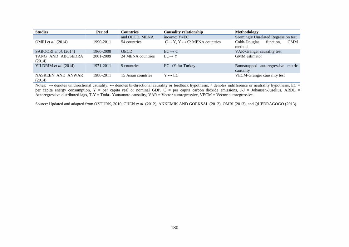
180

Studies Period Countries Causality relationship Methodology and OECD, MENA income: Y≠EC Seemingly Unrelated Regression test

OMRI et al. (2014) 1990-2011 54 countries C→ Y, Y ↔ C: MENA countries Cobb-Douglas function, GMM method

SABOORI et al. (2014) 1960-2008 OECD EC ↔ C VAR-Granger causality test TANG AND ABOSEDRA (2014)

2001-2009 24 MENA countries EC→ Y GMM estimator

YILDRIM et al. (2014) 1971-2011 9 countries EC→Y for Turkey Bootstrapped autoregressive metric causality

NASREEN AND ANWAR (2014)

1980-2011 15 Asian countries Y ↔ EC VECM-Granger causality test

Notes: → denotes unidirectional causality, ↔ denotes bi-directional causality or feedback hypothesis, ≠ denotes indifference or neutrality hypothesis, EC = per capita energy consumption, Y = per capita real or nominal GDP, C = per capita carbon dioxide emissions, J-J = Johansen-Juselius, ARDL = Autoregressive distributed lags, T-Y = Toda– Yamamoto causality, VAR = Vector autoregressive, VECM = Vector autoregressive. Source: Updated and adapted from OZTURK, 2010, CHEN et al. (2012), AKKEMIK AND GOEKSAL (2012), OMRI (2013), and QUEDRAGOGO (2013).

181

Appendix B – Table of key alternative indicators to GDP.

Table B 1 - Key alternative indicators to GDP.

Alternative Indicators

Year introduced

Approach to GDP EcD SD EnD

Number of countries covered

Period covered (years)

References

Measure of Economic Welfare (MEW) 1972 adjusting ✓ ✓ 1 36 NORDHAUS AND TOBIN, 1972

World Values Survey (WVS) 1984 replacing ✓ ✓ 80 33 DIENER AND SUH, 1997 Index for Sustainable Economic Welfare (ISEW) 1989 adjusting ✓ ✓ ✓ 14 29 DALY AND COBB, 1989

Human Development Index (HDI) 1990 replacing ✓ ✓ 188 24 UNDP, 1990, 2010, 2013, and 2015

Genuine Progress Indicator (GPI) 1995 adjusting ✓ ✓ ✓ 17 60 ANIELSKI AND ROWE 1999, TALBERTH et al., 2007, KUBISZEWSKI et al., 2013

Index of Economic Wellbeing (IEWB) 1998 adjusting ✓ ✓ ✓ 14 29 OSBERG AND SHARPE, 1998 and 2011

Happy Planet Index (HPI) 2006 replacing ✓ ✓ ✓ 151 6 MARKS et al., 2006

Sustainable Society Index (SSI) 2008 adjusting ✓ ✓ ✓ 151 8 VAN DE KERK AND MANUEL, 2014

The Legatum Prosperity Index 2009 adjusting ✓ ✓ ✓ 110 6 LEGATUM INSTITUTE, 2009 Human Sustainable Development Index (HSDI) 2010 replacing ✓ ✓ ✓ 188 1 TOGTOKH, 2011

Sustainable Economic Development Assessment (SEDA) 2011 adjusting ✓ ✓ ✓ 149 3 BEAL et al., 2015

Adjusted Net Savings (ANS) 2012 adjusting ✓ ✓ 144 13 WORLD BANK, 2013

Inclusive Wealth Indicator (IWI) 2012 adjusting ✓ ✓ ✓ 116 20 UNU-IHDP AND UNEP, 2012 and 2014

Social Progress Index (SPI) 2013 supplementing ✓ ✓ 133 2 PORTER et al., 2016

Note: EcD = Economic Dimension, SD = Social Dimension, and EnD = Environmental Dimension. Source: Prepared by the author based on data from GOOSSENS et al., 2007 and SCHEPELMANN et al., 2010, and own research.

182

Appendix C – Table of key data and calculations.

Table C 1 – Description of key data and calculations.

Data Description Sources Historic data Inclusive Wealth Index (IWI) (millions 2005 US$)

Social value of an economy's capital assets (e.g. natural, manufactured, humans, and social), seen as determinants of wellbeing and proxies to its actual constituents.

IWR 2014 (UNU-IHDP and UNEP, 2014)

Started with a list of 140 countries in IWR 2014, then eliminated those for which there were no energy consumption data in the World Bank database and arrived to 118 countries. Data provided for years 1990, 1995, 2000, 2005 and 2010 for all countries except for Croatia, Kazakhstan, Kyrgyzstan, Lithuania, Russian Federation, Slovenia, Tajikistan, and Ukraine (1991 data provided instead of 1990) and Czech Republic and Slovakia (1992 data provided instead of 1990). Data for intermediate years were calculated based on compound annual growth rates.

GDP, PPP (constant 2011 international $)

Gross domestic product converted to international dollars using purchasing power parity rates. An international dollar has the same purchasing power over GDP as the U.S. dollar has in the United States. GDP is the sum of gross value added by all resident producers in the economy plus any product taxes and minus any subsidies not included in the value of the products. It is calculated without making deductions for depreciation of fabricated assets or for depletion and degradation of natural resources. Data are in constant 2011 international dollars.

World Development Indicators (WORLD BANK, 2016)

Deflators used to convert GDP to 2005 US$

Implicit Price Deflators for Gross Domestic Product

Bureau of Economic Analysis (BEA) (https://bea.gov/itable/

Energy use (EU) (kg of oil equivalent per capita)

Energy use refers to use of primary energy before transformation to other end-use fuels, which is equal to indigenous production plus imports and stock changes, minus exports and fuels supplied to ships and aircraft engaged in international transport.


Energy consumption (EC)

EC = EU converted from koe into GJ: 1 GJ = 1 koe / 1000 x 41.868

OECD/IEA 2016 (https://www.iea.org/statistics/resources/unitconverter)

Population Total population is based on the de facto definition of population, which counts all residents regardless of legal status or citizenship--except for refugees not permanently settled in the country of asylum, who are generally considered part of the population of their country of origin. The values shown are midyear estimates.


183

Data Description Sources CO2 emissions Carbon dioxide emissions are those stemming

from the burning of fossil fuels and the manufacture of cement. They include carbon dioxide produced during consumption of solid, liquid, and gas fuels and gas flaring.


CO2 emission intensity

CO2 emissions / Energy use

Wellbeing Projections

Projected pcIWI = ((1 r) pcIWI)/Projected Pop

IWI growth rates

Projected growth rate (r) derived from observed IWI trend in each region for 1990-2010

IWR 2014 (UNU-IHDP and UNEP 2014)

Compound annual growth rate for 2005-2010 (last 5 years) used to project 2011-2020



Projected population

Projected population for each RC5 region based on population growth in the no-policy baseline emission scenario in the IAM MESSAGE. Calibrated to 2010, start of projections.

LIMITS Scenario database (public) (Version 1.0.0) https://tntcat.iiasa.ac.at/LIMITSPUBLICDB

Energy Projections

Projected EC = Projected pcEC x Projected Pop

Projected pcEC= EXP((LN(projected pcIWI) - a)/b)

EC/IWI elasticities (b)

Estimated from log-log regressions on cross-section data for 2010

2011-2050: projections based on EC/IWI elasticities estimated from log-log regressions on cross-section data for 2010

Decoupling rate Upper bound rates calculated based on prorated highest decrease rates observed, to be applied in 10-year period (2011-2020). Lower bound rates calculated based on prorated highest increase rates observed, to be applied in 10-year period (2011-2020). Second highest rates used to avoid distortions from peaks in EIT and LAM.

Projected population

Projected population for each RC5 region based on population growth in the IAM MESSAGE. Calibrated to 2010, start of projections.


CO2 Emissions Projections

Projected CO2 emissions = Projected EC x Projected CO2 emission intensities

Two series of projected CO2 emissions (based on lower bound and upper bound projected EC series) are calculated.

Projected CO2 emission intensities LOWER and UPPER bounds

Projected CO2 emission intensities = 2010 CO2 emission intensity X Growth rates

2010 CO2 intensity = 2010 CO2 emissions / 2010 World Development

184

Data Description Sources Energy Use (for each region) Indicators (WORLD

BANK, 2016) Growth rates Four sets of annualized intensities growth rates

for each region for the years 2011 through 2050 (2011-2020, 2021-2030, 2031-2040, 2041-2050) obtained from projected CO2 emissions from fossil fuel combustion and industrial processes and primary energy consumption levels also from the no-policy baseline scenario of the IAM MESSAGE.


Projected CO2 intensity = Projected CO2 emissions / Projected primary energy

Projected CO2 emissions in 450 and 500ppm scenarios were obtained from IAM MESSAGE 450 and 500ppm scenarios, normalized to 2010.

185

Appendix D – Table of region categorization.

Table D 1 - Region categorization. Region Countries in RC5 region* Countries not included in

this analysis % world pop

OECD90 Australia, Austria, Belgium, Canada, Denmark, Fiji, Finland, France, French

Polynesia, Germany, Greece, Guam, Iceland, Ireland, Italy, Japan, Luxembourg,

Netherlands, New Caledonia, New Zealand, Norway, Portugal, Samoa, Solomon Islands, Spain, Sweden,

Switzerland, Turkey, United Kingdom, United States of America, Vanuatu

French Polynesia, Guam, New Caledonia, Samoa,

Solomon Islands, Switzerland, Vanuatu

14

Economies in transition (EIT)

Albania, Armenia, Azerbaijan, Belarus, Bosnia and Herzegovina, Bulgaria,

Croatia, Cyprus, Czech Republic, Estonia, Georgia, Hungary, Kazakhstan,

Kyrgyzstan, Latvia, Lithuania, Malta, Poland, Republic of Moldova, Romania, Russian Federation, Slovakia, Slovenia,

Tajikistan, TFYR Macedonia, Turkmenistan, Ukraine, Uzbekistan,

Yugoslavia

Azerbaijan, Belarus, Bosnia and Herzegovina,

TFYR Macedonia, Uzbekistan, Yugoslavia

5

Asia (ASIA)

Afghanistan, Bangladesh, Bhutan, Brunei Darussalam, Cambodia, China, Hong Kong, Macao, Democratic People's

Republic of Korea, East Timor, India, Indonesia, Lao PDR, Malaysia, Maldives,

Mongolia, Myanmar, Nepal, Pakistan, Papua New Guinea, Philippines, Republic of Korea, Singapore, Sri Lanka, Taiwan,

Thailand, Viet Nam

Afghanistan, Bhutan, Brunei, Hong Kong,

Macao, Korea DRP, East Timor, Lao PDR,

Maldives, Papua New Guinea, Taiwan.

52

Middle East and Africa (MAF)

Algeria, Angola, Bahrain, Benin, Botswana, Burkina Faso, Burundi,

Cameroon, Cape Verde, Central African Republic, Chad, Comoros, Congo, Cote

d'Ivoire, Democratic Republic of the Congo, Djibouti, Egypt, Equatorial

Guinea, Eritrea, Ethiopia, Gabon, Gambia, Ghana, Guinea, Guinea-Bissau, Iran

(Islamic Republic of), Iraq, Israel, Jordan, Kenya, Kuwait, Lebanon, Lesotho, Liberia, Libyan Arab Jamahiriya,

Madagascar, Malawi, Mali, Mauritania, Mauritius, Morocco, Mozambique,

Namibia, Niger, Nigeria, Oman, Qatar, Reunion, Rwanda, Saudi Arabia, Senegal,

Sierra Leone, Somalia, South Africa, Sudan, Swaziland, Syrian Arab Republic,

Togo, Tunisia, Uganda, United Arab Emirates, United Republic of Tanzania,

Western Sahara, Yemen, Zambia, Zimbabwe

Angola, Burkina Faso, Burundi, Cape Verde, Central African Rep.,

Chad, Comoros, Congo, Djibouti, Equatorial

Guinea, Eritrea, Ethiopia, Guinea, Guinea-Bissau,

Lebanon, Lesotho, Liberia, Libyan Arab Jamahiriya,

Madagascar, Malawi, Mali, Mauritania,

Mauritius, Namibia, Niger, Oman, Reunion, Rwanda,

Sierra Leone, Somalia, Swaziland, Uganda, United Republic of

Tanzania, Western Sahara

13

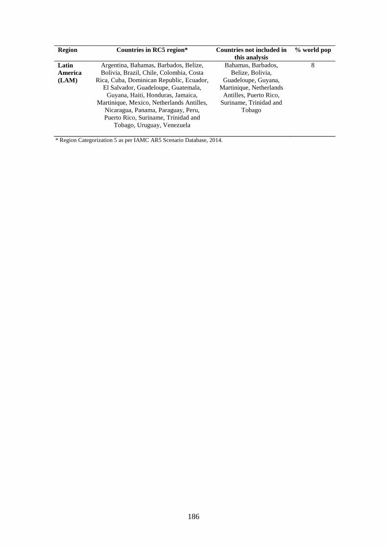
186

Region Countries in RC5 region* Countries not included in this analysis

% world pop

Latin America (LAM)

Argentina, Bahamas, Barbados, Belize, Bolivia, Brazil, Chile, Colombia, Costa

Rica, Cuba, Dominican Republic, Ecuador, El Salvador, Guadeloupe, Guatemala,

Guyana, Haiti, Honduras, Jamaica, Martinique, Mexico, Netherlands Antilles,

Nicaragua, Panama, Paraguay, Peru, Puerto Rico, Suriname, Trinidad and

Tobago, Uruguay, Venezuela

Bahamas, Barbados, Belize, Bolivia,

Guadeloupe, Guyana, Martinique, Netherlands

Antilles, Puerto Rico, Suriname, Trinidad and

Tobago

8

* Region Categorization 5 as per IAMC AR5 Scenario Database, 2014.

187

Appendix E – Comparison with previous quantification efforts.

Based on the findings of this study, the four regions combined, representing 78

percent of global population (based on 2010 data), would require between 606-897 EJ

per year and between 42.1 and 62.8 GtCO2 per year by 2050 (Table 7), as well as

17,264 and 24,216 EJ of cumulative energy consumption and between 1,174 and 1,658

GtCO2 of cumulative carbon emissions from 2011 to 2050 (Table 8) to achieve higher

collective wellbeing. These refer to average primary energy consumption rates of

approximately 78 to 116 GJ per capita by 2050.

PASTERNAK (2000) had estimated a range from 378 to 492 EJ of overall

primary energy consumption needed to reach a global average primary energy

consumption rate of approximately 108 GJ per capita.122 UGURSAL (2014) had

estimated about 419 EJ (or 10 billion toe) of additional energy consumption needed to

reach a global average energy consumption rate of 105 GJ per capita. According to

PASTERNAK (2000) this rate would be achieved in 2020 while, according to

UGURSAL (2014), it would only be achieved by 2100. Notwithstanding the different

timeframes, those estimates are at least 19 percent lower than those obtained in this

study.

COSTA et al. (2011) applied historic correlations between HDI and per capita

CO2 emissions (from fossil fuels combustion) to estimate the carbon impact of reaching

specific HDI thresholds. They estimated that between 850 and 1,100 GtCO2 of

cumulative CO2 emissions between 2000 and 2050 would be needed for 85 percent of

the total world population to achieve a minimum of 0.8 HDI by 2050. These estimates

are considerably lower than those obtained in this study (1,174 and 1,658 GtCO2

between 2011 and 2050), in particular considering the 9 years difference (projections

start in 2000, as opposed to 2011 in the present study) and the small difference in the

sample size (85 percent of total world population, contrasted with 78 percent in the

present study).

122 This range refers to achieving a minimum of 4,000 kWh (or 14.4 GJ) per capita electricity consumption or an estimated (at 7.5 ratio) 108 GJ (or 2580 koe) per capita primary energy consumption.

188

LAMB AND RAO (2015) projected energy requirements and corresponding

CO2 emissions of reaching minimum thresholds in two dimensions of human wellbeing

(social and economic) in three developing regions (Africa, Centrally Planned Asia, and

South Asia) that together represent 67 percent of the world population (based on 2010

data). They employed a composite of six factors related to food, shelter, basic health

and hygiene, and education, as well as the UN’s life expectancy data as proxy

measurements for the social dimension of human development. They used GDP per

capita data as proxy for the economic dimension.

They estimated approximately 216 GtCO2eq of cumulative CO2 emissions

would be required to achieve minimum social wellbeing levels between 2011 and 2050

in Africa (up to 54 GJ/capita/year final energy consumption rate by 2050), 442

GtCO2eq in Centrally Planned Asia (up to 45 GJ/capita/year by 2050), and 345

GtCO2eq in South Asia (up to 44 GJ/capita/year by 2050). The three regions combined,

representing 67 percent of the world population (based on 2010 data), would require a

total of just over 1,000 GtCO2eq between 2011 and 2050.

Given the different regional aggregation, we can only compare the results from

LAMB AND RAO (2015) for Asia with those obtained for the same region in this

study. While they provide an estimate for Africa, in the present analysis Africa is

included in MAF (Middle East and Africa), therefore the numbers are not directly

comparable. See Appendix D for the region categorization used in this study.

According to their findings, Asia (Centrally Planned Asia and South Asia)

would require 787 Gt GtCO2eq to achieve minimum social wellbeing levels, reaching a

final energy consumption rate of up to about 45 GJ per capita by 2050. It is noteworthy,

that LAMB AND RAO (2015) calculated emissions as a sum of all greenhouse gases

for each region, only excluding GHG emissions associated with land-use change. In the

present study, in contrast, only CO2 emissions from fossil fuels and industry were taken

in to account, which represent about 66 percent of all GHG emissions (excluding land

use) in the LIMITS baseline run 2010 data. As such, their estimates for Asia would

equate very roughly to about 519 GtCO2.

However, it is also important to highlight that LAMB AND RAO (2015) used

189

final energy consumption data while the present study used primary energy

consumption data. Recalling that final energy refers to the conversion of primary energy

sources into energy ready for transportation or transmission, and that in every

conversion step some energy is always lost, final energy levels are always expected to

be lower than the associated primary energy from which they derived. Final energy

consumption per capita rates in Asia averaged roughly 70 percent of primary energy

consumption rates over the 1990-2010 period (UNESCAP, 2017). As such, their

estimates for Asia (519 GtCO2) could equate roughly to a 64 GJ per capita primary

energy consumption rate or to an emissions intensity rate of 8.1 GtCO2/GJ.

Taken all these differences into account, the estimates for Asia in LAMB AND

RAO (2015) are comparable to the range of 817 to 1,192 GtCO2 of cumulative

emissions from 2011 to 2050 associated with reaching primary energy consumption

rates of 94 to 146 GJ per capita estimated in the present study, or emissions intensity

rates of 8.2 to 8.7 GtCO2/GJ. Therefore, their estimates for Asia are at least 36 percent

lower than those obtained in this study.

190

Appendix F – Assessing the gaps in all regions (including OECD90).

Table F.1 presents the emissions shortfalls (gaps) between the 450-ppm carbon

budget (i.e. associated with reasonably high chance of limiting the temperature increase

to below 2 oC) and the estimated additional carbon emissions (projected CO2 emissions)

associated with future improvements in human wellbeing in all 5 regions (including

OECD90) by 2050,123 in all emissions scenarios considered.

Table F 1 - Emissions shortfall by 2050 per emissions scenario compared to the

450-ppm budget.

Region/ Scenario


Gap in No-action

scenario

Gap in Delayed

action-500 scenario

Gap in Action as of

2020-500 scenario

Gap in Action as of

2020-450 scenario

at least up to at


least up to

ASIA 421 396 771 207 484 170 429 82 296

MAF 112 51 71 23 40 4 17 (9) 3

LAM 48 32 78 6 35 (8) 13 (11) 8

EIT 75 40 83 10 40 2 29 (8) 15

OECD90 256 155 268 53 134 46 161 8 75

Total all regions 912 674 1,271 298 732 214 649 62 397


Table F.2 presents all gaps between the 500-ppm carbon budget (i.e. associated

with even chance of limiting the temperature increase to below 2 oC) and the estimated

additional carbon emissions (projected CO2 emissions) associated with future

improvements in human wellbeing in all 5 regions (including OECD90) by 2050, in all

emissions scenarios considered.

123 Future levels of wellbeing in OCDE90 were projected following the same criteria applied to the other regions until 2020 (section 4.3), thereafter it was assumed constant on a per capita basis (pcIWI).

191

Table F 2 - Emissions shortfall by 2050 per emissions scenario compared to the

500-ppm budget.

Region/ Scenario


Gap in No-action

scenario

Gap in Delayed

action-500 scenario

Gap in Action as of

2020-500 scenario

Gap in Action as of

2020-450 scenario

at least up to at


least up to

ASIA 527 291 665 101 378 64 323 (24) 190

MAF 128 35 55 7 24 (12) 1 (25) (13)

LAM 57 22 68 (4) 25 (17) 3 (21) (2)

EIT 91 24 67 (6) 24 (13) 14 (23) (0)

OECD90 308 104 216 1 82 (6) 109 (43) 24

Total 4 regions 1,111 475 1,072 99 533 15 450 (136) 198


Even if new climate policies and mitigation actions associated with reasonably

high chances of meeting the 2 oC target, i.e. reaching GHG concentrations at roughly

450 ppm CO2eq in 2100, were adopted in all four regions where improvements are still

needed as well as in advanced countries (OECD90 region) in 2020, emissions

associated with meeting the urgent energy needs while enabling the achievement of

higher levels of collective wellbeing, could still exceed both estimated carbon budgets,

the 450-ppm and the 500-ppm, by almost one and a half times (i.e. a gap of 397 GtCO2)

and by over one time (i.e. a gap of 198 GtCO2), respectively, by mid-century.

Documents

BRIDGING THE ENERGY DIVIDE AND SECURING HIGHER … · Gabriela, Gabriela L., Kristen, Monika, and Rina for all the support and encouragement received throughout the development of