Todos os direitos reservados. É proibida a reprodução parcial ou integral do conteúdo

deste documento por qualquer meio de distribuição, digital ou impresso, sem a expressa autorização do

REAP ou de seu autor.

Coordination in the Use of Money

Luis Araujo

Bernardo Guimaraes

Julho, 2012 Working Paper 044

COORDINATION IN THE USE OF MONEY

Luis Araujo Bernardo Guimaraes

Luis Araujo Michigan State University Fundação Getúlio Vargas Departamento de Economia Escola de Economia (EESP/FGV) 220A Marshall-Adams Hall East Lansing, MI – Estados Unidos araujolu@msu.edu Bernardo Guimaraes Fundação Getúlio Vargas Escola de Economia de São Paulo (EESP/FGV) Rua Itapeva, nº 474 01332-000 - São Paulo, SP - Brasil bernardo.guimaraes@fgv.br

Coordination in the use of money�

Luis Araujoy Bernardo Guimaraesz

Abstract

Fundamental models of money, while explicit about the frictions that render money socially

bene�cial, are silent on how agents actually coordinate in its use. This paper studies this

coordination problem, providing an endogenous map between the primitives of the environment

and the beliefs on the acceptability of money. We show that an increase in the frequency of

trade meetings, besides its direct impact on payo¤s, facilitates coordination. In particular,

for a large enough frequency of trade meetings, agents always coordinate in the use of money.

We highlight the underlying properties of money (medium of exchange, record-keeping) that

facilitate coordination.

Key Words: Money, Beliefs, Coordination.

JEL Codes: E40, D83

�We thank Federico Bonetto, Gabriele Camera, Raoul Minetti, Stephen Morris, Daniela Puzzello, Randy Wright,Tao Zhu and seminar participants at Dauphine, ESSIM 2011, Michigan State, Rochester, SAET Meeting 2011, SãoPaulo School of Economics-FGV and the 2011 Summer Workshop on Money, Banking, Payments and Finance at theFederal Reserve Bank of Chicago for their comments and suggestions.

yCorresponding Author. Michigan State University, Department of Economics, and São Paulo School ofEconomics-FGV. E-mail address: araujolu@msu.edu.

zSão Paulo School of Economics-FGV.

1

1 Introduction

The principle that the use of money should be explained by its essentiality is well established among

monetary theorists.1 A precise description of the frictions (e.g., limited commitment, limited record-

keeping) that render money necessary if the economy is to achieve socially desirable allocations is a

crucial element in models where the use of money is not taken as a primitive of the environment.2

However, these models take the belief that money is accepted as given, thus assuming away the

coordination problem involved in its use. In this paper we step towards �lling this gap by exploring

how the primitives of the economy and the underlying properties of money impact agents�ability

to coordinate in its use.

We cast our analysis in a search model of money along the lines of Kiyotaki and Wright (1993).

The key departure from their environment is the assumption that money is not completely �at.

We let the economy experience di¤erent states over time and assume that, while money is �at in

a large region, there exist faraway states where money acquires negative intrinsic utility (and it

becomes a strictly dominant action not to accept money) and faraway states where money acquires

positive intrinsic utility (and it becomes a strictly dominant action to accept money). A precise

interpretation of how money may acquire some intrinsic disutility or utility is not important in

our analysis, but we think of di¤erent states as re�ecting changes in the physical characteristics of

money or changes in the characteristics of the environment that may impact the e¤ectiveness of

money as a medium of exchange. What is important is that the existence of remote states where

either accepting or not accepting money is a strictly dominant action prevents the emergence of

equilibria where an agent chooses a particular action because he is certain everyone else will always

choose the same action in all possible states. This restriction on beliefs allows us to derive a link

between the primitives of the economy and agents�beliefs on the acceptability of money.

We �rst show that if there are enough gains from trade, agents always coordinate in the use of

money in the region where it is completely �at. This result, albeit novel to monetary economies,

is analogous to those found in other settings with strategic complementarities where agents cannot

coordinate in the same particular set of beliefs in all states of the world. More interestingly, we

decompose the impact of an increase in the time discount factor (or an increase in the frequency

of trade meetings) on the acceptability of money into two channels: an e¢ ciency channel, which

takes the belief that money is accepted by the other agents as given; and a coordination channel,

which considers how an increase in the frequency of trade meetings a¤ects the beliefs of an agent

about the acceptability of money in states where it has no intrinsic utility. As the frequency of

trade meetings increases, the region of parameters where agents coordinate in the use of money

expands, and in the limit where the frequency of trade meetings goes to in�nity, agents coordinate

in the use of money if and only if it is e¢ cient to do so.

1For a discussion of the notion of essentiality, see Kocherlakota (1998) and Wallace (2001).2Key references are Kiyotaki and Wright (1989, 1993), Trejos and Wright (1995), Shi (1995, 1997), and Lagos and

Wright (2005).

2

The result that the e¢ cient outcome always emerges when agents become in�nitely patient un-

veils a distinctive feature of the coordination problem involved in the use of money. Two properties

of money are particularly important. First, the decision to accept money is not made once but

many times. Thus, if an agent exerts e¤ort in order to earn money today, he will be able to spend

it sooner, and consequently further opportunities to accept and spend money will also come sooner.

The more patient the agent is, the more value he gives to such future opportunities. Second, money

is a durable form of record-keeping, i.e., it is evidence that, at some point in the past, no matter

how far back it is, an agent produced to someone else, and is thus entitled to current consumption.

This ensures that a patient agent will be willing to exert e¤ort in exchange for money even if he

believes that it will take a long time until he can spend money, which gives rise to beliefs that

money will be widely accepted in the economy.

Our paper relates to the literature on equilibrium selection in dynamic games with complete

information, in particular, Frankel and Pauzner (2000) (FP), and Burdzy, Frankel, and Pauzner

(2001) (BFP).3 We share with these papers both the assumption that there exist faraway states

where it is strictly dominant to choose a particular action and the result that the ensuing equilibrium

is unique.4 An important di¤erence is that in FP and BFP, an increase in the time discount factor

does not help selecting the e¢ cient outcome. In their model, if the time discount factor is large

enough, the risk-dominant equilibrium is selected regardless of whether it is e¢ cient. This underpins

our argument that, thanks to the underlying properties of money, the coordination problem involved

in its use is markedly di¤erent from that present in other, non-monetary, settings.

Finally, there is a strand of models within monetary economics that studies how the addition

of an intrinsic utility to money may help to reduce the set of equilibria. In overlapping generations

models, the focus is on the elimination of monetary equilibria that exhibit in�ationary paths (Brock

and Scheinkman (1980), Scheinkman (1980)). In search models of money, the objective is to

characterize the set of �at money equilibria that are limits of commodity-money equilibria when

the intrinsic utility of money converges to zero (Zhou (2003), Wallace and Zhu (2004), Zhu (2003,

2005)). A result that comes out of this work is that, if goods are perfectly divisible and the marginal

utility is large at zero consumption, autarky is not the limit of any commodity money equilibria.

This result critically depends on the assumption that there is a su¢ ciently high probability that

the economy reaches a state where �at money acquires an intrinsic utility. In contrast, our results

hold even if the probability that money ever acquires intrinsic utility is arbitrarily small and the

probability that it ever acquires intrinsic disutility is equal to one. Most importantly, this literature

3 It is also related to the literature on equilibrium selection in games with incomplete information, surveyed byMorris and Shin (2003).

4One relevant di¤erence is that in a monetary economy, the bene�t of exerting e¤ort in exchange for moneydepends on how agents will behave in the near future and not on how they behave today. This eliminates equilibriain which an agent chooses a particular action in a given period simply because he believes that all the other agents willchoose the same action in that period. In order to deal with this problem, FP and BFP assume that each agent hasonly a small chance of changing his action in any given period in order to prevent the multiplicity of equilibria thatarises when agents are allowed to continuously shift from one action to another. We do not need an extra assumptionto tackle this issue.

3

does not explain (it is not meant to) how the fundamentals of the economy and the underlying

properties of money a¤ect the ability to coordinate in its use.

The paper is organized as follows. In section 2, we present the model, deliver our main result,

and discuss our assumptions. In section 3, we examine how the frequency of trade meetings and

the underlying properties of money impact agents�ability to coordinate in its use. In section 4, we

conclude. The appendix contains proofs omitted from the main text.

2 Model

2.1 Environment

Our environment is a version of Kiyotaki and Wright (1993). Time is discrete and indexed by t.

There are k indivisible and perishable goods and the economy is populated by a unit continuum of

agents uniformly distributed across k types. A type i agent derives utility u per unit of consumption

of good i and is able to produce one unit of good i + 1 (modulo k) per period, at a cost c < u.

Agents maximize expected discounted utility with a discount factor � 2 (0; 1). There is a storableand indivisible object, which we call money. An agent can hold at most one unit of money at a

time, and money is initially distributed to a measure m of agents.

Trade is decentralized and there are frictions in the exchange process. There are k distinct

sectors, each one specialized in the exchange of one good. In every period, agents choose which

sector they want to visit but inside each sector they are randomly and pairwise matched. Each

agent faces one meeting per period, and meetings are independent across agents and independent

over time. Thus if an agent wants money, he goes to the sector which trades the good he produces

and searches for an agent with money. If he has money, he goes to the sector which trades the good

he likes and searches for an agent with the good.

In any given period, the economy is in some state z 2 R. The economy starts at z = 0 and

the state changes according to a random process zt+1 = zt +�zt, where �zt follows a continuous

probability distribution that is independent of z and t, with expected value E(�z) � 0 and varianceVar(�z) > 0. The state of the economy does not a¤ect the preferences for goods and the production

technology. However, it may a¤ect the intrinsic utility of money: there exists a state bz > 0 and afunction (z) such that (1) if z < �bz, money provides an intrinsic utility (z) < 0; (2) if z 2 [�bz; bz],money provides no intrinsic utility, i.e., (z) = 0; and (3) if z > bz, money provides an intrinsicutility (z) > 0.

Throughout, we assume that bz is �nite but very large, and we are interested in describing howagents behave in states where money provides no intrinsic utility. The probability that states below

�bz and states above bz will ever be reached depends on the stochastic process of �z. If E(�z) iszero, both �bz and bz will eventually be reached with probability one. If, instead, E(�z) is slightlynegative, the probability that bz will ever be reached depends on how far z = 0 is from bz. In

4

particular, by choosing a large enough bz, we can make the probability that money ever acquires apositive intrinsic utility as small as we want. In what follows we show that we can choose E(�z)

to make the probability of reaching either of the faraway states where money starts acquiring some

intrinsic utility arbitrarily small, with virtually no e¤ect in any of our results. We will return to

this claim in section 2.4.

The Intrinsic Utility of Money The possibility that money may deliver a positive or a negative

intrinsic utility is the key dimension in which our model departs from a standard search model of

money. We think of the state of the economy as re�ecting the physical characteristics of money.

In most states money is intrinsically useless. This is captured by the assumption that the intrinsic

utility of money is equal to zero if z 2 [�bz; bz], and by the fact that bz can be as large as we want, aslong as it is �nite. However, there are (faraway) states where accepting money entails a cost due

to changes in its physical properties. For example, money may become more costly to carry.5 We

capture this idea by assuming that accepting money in a state z < �bz gives to the agent a �owutility < 0. In turn, there are (faraway) states where changes in the physical properties of money

can turn it into a desirable good in and of itself. For example, one can think of the development

of a technology that can convert money into a shiner object, say a jewel. We capture this idea by

assuming that if an agent holds one unit of money at the beginning of a period in a state z > bz, hecan convert this unit into an intrinsically desirable object, in which case he obtains utility > 0.

The only objective of allowing for an intrinsic utility to money is to introduce states in which

accepting money is either a strictly dominant or a strictly dominated action. There are many ways

in which this can be done. In what follows, we ensure that money is never accepted if z < �bz byassuming that < ��u. Now, in order to ensure that money is always accepted in states z > bz,we need to consider the expected bene�t of holding money at the end of a period under the belief

that money will never be accepted by the other agents. In this case, since the bene�t of money

only comes from the possibility of converting it into an intrinsically desirable object upon reaching

some state z > bz in a future period, the agent needs to take into account how states evolve overtime, as given by the random process �zt. If we denote by '(t) the probability that any state

z0 > z is reached in period s+ t and not before, conditional on the agent being in state z in period

s, money is accepted in all states z > bz ifX1

t=1�t'(t) > c.6 Finally, we want to make it clear

that the dominant role of money comes from its use as a medium of exchange and not from its

intrinsic utility, i.e., even if money may have some intrinsic utility, the agent still prefers to use

it as a medium of exchange if he believes that other agents will do the same. For this reason, we

further assume that [1�mX1

t=1�t'(t)] < (1�m)u.7 In section 2.4 we argue that a more general

5Alternatively, accepting money may become costly due to changes in the environment that increase the transactioncosts of using money.

6An agent that accepts money at bz will get �t� after t periods with probability ' (t). An agent at z > bz will onaverage get � sooner, hence his incentives for accepting money are larger.

7An agent that converts his unit of money in a �jewel�gets � and leaves the game. A lower bound for the payo¤ of

5

speci�cation of the function (z) would not a¤ect the substantive results of the paper.

2.2 Benchmark case

We initially consider the benchmark case where bz = 1 and money is completely �at. We are

interested in the behavior of an agent without money, who is asked to produce in exchange for

money. The decision of an agent on whether to o¤er money in exchange for a desirable good is

trivial in our model, since the most an agent can obtain with one unit of money is one unit of good,

and all desirable goods provide the same utility u.

In principle, the behavior of an agent may depend on the history of states and, consequently, on

the agent�s belief about the behavior of all other agents in all future periods, and after every possible

history of states. A natural approach though if money is completely �at is to look at equilibria

where agents�behavior do not depend on the history of states. One such equilibrium is autarky,

where each agent believes all other agents will never accept money. Under some conditions on

parameters, another equilibrium is money, in which each agent believes all other agents will always

accept money.

Let V1;z be the value function of an agent with money in state z if he believes all other agents

will always accept money, and let V0;z be de�ned in a similar way for an agent without money. We

have

V1;z = m�EzV1 + (1�m) (u+ �EzV0) ,

and

V0;z = m [� (�c+ �EzV1) + (1� �)�V0] + (1�m)�EzV0,

where �EzV1 is the expected payo¤ of carrying one unit of money into the next period, �EzV0is the expected payo¤ of carrying zero units of money into the next period, and � 2 [0; 1] is theprobability that the agent accepts money. Consider the expression for V1;z. An agent with money

goes to the sector that trades the good he likes. In this sector, there is a probability m that he

meets another agent with money and no trade happens. There is also a probability (1 �m) thathe meets an agent without money, in which case they trade, the agent obtains utility u, and moves

to the next period without money. A similar reasoning holds for an agent without money.

Assume that � = 1. This implies that, for all z,

V1;z � V0;z = (1�m)u+mc.

It is indeed optimal to always accept money as long as �c+ �V1;z � �V0;z, i.e.,

� [(1�m)u+mc] � c. (1)

an agent that decides to take money to the market is given by the probability of meeting someone who produces thegood he likes times the bene�t of getting the good, (1�m)u, plus the probability of meeting another buyer insteadof a seller (m) times the value of starting next period with money. A lower bound for the value of money in this caseis given by

X1

t=1�t'(t) , since the agent can convert money in a �jewel�whenever he is in a state z > bz, and as

discussed in the previous footnote,X1

t=1�t'(t) is a lower bound for the expected value of money in this case.

6

Thus, if money is completely �at and (1) holds, there always exist an autarkic equilibrium and

a monetary equilibrium.8

2.3 General case

We now consider the case where bz is �nite, so there are states where money carries some intrinsicutility. We are interested in the behavior of agents without money who are asked to produce in

exchange for money in states where money yields no intrinsic utility. In what follows, we focus

on equilibria in cut-o¤ strategies, i.e., strategies where an agent accepts money if and only if the

current state is above some threshold state z�, where z� 2 [�1;1]. To be clear, we do not imposethat agents have to follow a cut-o¤ strategy, we allow for deviations where an agent chooses a

strategy that is not of a cut-o¤ type. Proposition 1 summarizes our main result.

Proposition 1 Let bz 2 R and X1

t=1�t'(t) [(1�m)u+mc] > c. (2)

Then, there exists a unique equilibrium in cut-o¤ strategies. In this equilibrium, money is accepted

if and only if z � �bz.Proposition 1 shows that, unless accepting money implies an intrinsic disutility, agents will

always coordinate in the use of money if (2) holds.9 The proof of Proposition 1 is organized in two

steps. First, taking beliefs about the behavior of others as given, we study the decision of an agent

and the relevant value functions. We then characterize the unique equilibrium in cut-o¤ strategies.

We start by showing that if an agent believes that all the others are following a cut-o¤ strategy

at z 2 [�bz; bz], then the best response is also a cut-o¤ strategy. This best response is unique andwe denote the corresponding cut-o¤ state by Z(z). This is proved in Lemma 1.

Lemma 1 For every z� 2 [�bz; bz], there exists a unique Z(z�) 2 [�bz; bz] such that, if an agentbelieves that all the other agents follow a cut-o¤ strategy at z�, then he produces in exchange for

money if and only if z � Z(z�).

Proof. See the Appendix.

The decision about accepting money is actually a decision between an action and an option.

The agent can accept money now, which entails a cost c but gives him money that can be used to

buy the good he likes next period. Alternatively, the agent can wait for another opportunity. The

8Kiyotaki and Wright (1993) show that there exists an equilibrium where agents are indi¤erent between acceptingand not accepting money. In this (unstable) mixed strategy equilibrium, the probability of accepting money isincreasing in c and decreasing in u. A similar equilibrium also exists here.

9The case where (2) holds with equality is uninteresting as it only occurs in a set of parameters with measurezero. We discuss the case where the reverse of (2) holds in section 2.4.

7

value of accepting money now and the value of the option of accepting money in the next period

are both increasing in the likelihood that money will be accepted later.

By accepting money in the current period, an agent puts himself in the position of getting

a reward at the �rst time the economy reaches a state where money is accepted by others. By

delaying the moment of accepting money, the agent saves in e¤ort cost, because the present value

of future e¤ort cost is lower than c, but the agent might miss on an opportunity to spend money

quickly. If an agent believes that all other agents are following a cut-o¤ strategy at some state

z�, and z is much larger than z�, it makes sense to accept money now, as the probability of a

reward in the following period is relatively high. In contrast, if z is much smaller than z�, it makes

more sense to wait for a future opportunity of accepting money, since there will probably be other

opportunities of accepting money before the agent can spend it. Lemma 1 shows that this intuition

applies more generally: if others are following a cut-o¤ strategy at some state z�, the payo¤ of

accepting money for an agent is increasing in z. Hence, the best response to cut-o¤ strategies is

also a cut-o¤ strategy.

Now let V1(z1; z2; z3) be the payo¤ of having money at the end of the period if the current state

is z1, all the other agents are following a cut-o¤ strategy at z2, and the agent is following a cut-o¤

strategy at z3 and let V0(z1; z2; z3) be the payo¤ of having no money in the same situation. Then

the net expected payo¤ of producing in exchange for money is given by

�c+ �V1(z1; z2; z3)� �V0(z1; z2; z3).

Lemma 2 shows that if an agent is following a cut-o¤ strategy at z 2 [�bz; bz] and all other agents arefollowing a cut-o¤ strategy at z0 2 [�bz; bz], then the net expected payo¤ of producing in exchangefor money in state z is strictly decreasing in z0.

Lemma 2 For any z and z0 in [�bz; bz], the net expected payo¤ of producing in exchange for money�c+ �V1(z; z0; z)� �V0(z; z0; z) is strictly decreasing in z0.

Proof. See the Appendix.

The intuition for Lemma 2 is similar to the intuition for Lemma 1: as the threshold for accepting

money z0 increases, the likelihood that money will be accepted by others in the near future decreases,

hence incentives for delaying the moment of producing in exchange for money increase.

Lemma 3 then uses Lemmas 1 and 2 to show that if an agent believes all others are following

a cut-o¤ strategy at z, then his expected payo¤ employing the same cut-o¤ strategy is su¢ cient to

determine the optimal behavior in state z.

8

Lemma 3 For any z 2 [�bz; bz], if� [V1(z; z; z)� V0(z; z; z)] > c, (3)

it is optimal to accept money in state z. If the inequality is reversed, then it is optimal not to accept

money in state z.

Proof. See the Appendix.

The key element in the proof of Lemma 3 is the fact that, since the random process �zt follows

a continuous probability distribution that is independent of the current state z, it must be that for

all z and z0 in [�bz; bz],V1(z; z; z)� V0(z; z; z) = V1(z0; z0; z0)� V0(z0; z0; z0).

In words, once everyone is following the same cut-o¤ strategy at some state in [�bz; bz], payo¤s donot depend on how far the cut-o¤ state is from the dominant regions. Thus a corollary of Lemma

3 is that if (3) holds, there exists an equilibrium in which all agents follow a cut-o¤ strategy at

z = �bz: the assumption that (z) < ��u for all z < �bz implies it is strictly optimal not to acceptmoney in all states z < �bz, and (3) implies it is strictly optimal to accept money in all states z � bzif agents are following a cut-o¤ strategy around bz. A similar reasoning implies that, if the reverseof (3) holds, there exists an equilibrium in which all agents follow a cut-o¤ strategy at z = bz.

Moreover, there can be no symmetric equilibrium in which agents follow a cut-o¤ strategy at

some state z 2 (�bz; bz). If (3) holds and all other agents are following a cut-o¤ strategy at somez 2 (�bz; bz), then Lemma 2 implies that the agent�s best response is to follow a cut-o¤ strategy atsome z0 < z. Similarly, if the reverse of (3) holds and all the other agents are following a cut-o¤

strategy at some z 2 (�bz; bz), then Lemma 2 implies that the agent�s best response is to follow acut-o¤ strategy at z0 > z.

Summing up, if one restricts attention to symmetric cut-o¤ strategies, there exists a unique

equilibrium. How about equilibria in which agents follow distinct cut-o¤ strategies? Lemma 4

proves that such equilibria cannot exist.

Lemma 4 There are no equilibria where agents follow di¤erent cut-o¤ strategies.

Proof. See the Appendix.

The intuition for Lemma 4 is that agents following di¤erent cut-o¤ strategies would have di¤er-

ent payo¤s: one agent would be accepting money even around states where others do not accept it,

while another one would only accept money when surrounded by states where money is accepted

by many others, but they cannot both be indi¤erent between accepting and not accepting money.

Hence in order to characterize behavior in the unique equilibrium in cut-o¤ strategies as a

function of the primitives, it is su¢ cient to consider payo¤s induced by a symmetric strategy pro�le

9

where all agents choose the same cut-o¤ z. Consider then the problem of an agent in state z in

period s. If he follows a cut-o¤ strategy at z and believes all others follow the same cut-o¤ strategy,

the net expected payo¤ of holding one unit of money at the end of period s, V1(z; z; z)�V0(z; z; z),is given by X1

t=1�t'(t)

�R1z

�V1;z0 � V0;z0

�dF (z0jt)

�. (4)

In words, conditional on the belief that money is only accepted in states z0 > z, the net expected

payo¤ of holding money is given by the discounted probability that the �rst time the economy

reaches some state z0 > z after period s happens in period s+t (which is given by �t'(t)) multiplied

by the net expected value of having money in state z0, that is, the expected value of V1;z0 � V0;z0 .The cdf of z0 is given by F (z0jt), i.e., the probability that the state of the economy is below or

equal to z0 conditional on the event that the �rst time the economy reaches some state z0 > z after

period s happens in period s+ t.

Now, if an agent follows a cut-o¤ strategy at z and if he believes that all the other agents follow

the same cut-o¤ strategy, the value of having money in some state z0 > z is given by

V1;z0 = m�Ez0V1 + (1�m) (u+ �Ez0V0) , (5)

while the value of not having money in some state z0 > z is

V0;z0 = m (�c+ �Ez0V1) + (1�m)�Ez0V0. (6)

The expected values Ez0V0 and Ez0V1 are complicated objects, but the analysis is vastly simpli�ed

because for any z0 > z

V1;z0 � V0;z0 = (1�m)u+mc. (7)

We can then substitute (7) in (4) and rewrite (3) asX1

t=1�t'(t) [(1�m)u+mc] > c.

which is the condition in (2).

2.4 Discussion

The condition in (2) holds for any bz 2 R. The role of the regions z > bz and z < �bz is simply tointroduce states where accepting money is either a strictly dominant or a strictly dominated action.

In particular, bz can be as large as we want, and it is in this sense that we think of the states wheremoney acquires a negative or a positive intrinsic utility as being faraway states.

An implication of (2) is that coordination in the use of money in states where money is com-

pletely �at does not depend on the actual values of and in the faraway states, irrespective of

the distance between the current state and the frontier states �bz and bz. This result hinges on theway the intrinsic utility of money was introduced in our model. The value of does not matter

10

even if the agent is at �bz because an agent only faces some disutility if he accepts money. Sincemoney is not accepted in states z < �bz, no agent actually incurs such disutility on the equilibriumpath. In turn, the value of does not matter even if the agent is at bz due to the assumptionthat [1 � m

X1

t=1�t'(t)] < (1 � m)u : if the agent is certain that money will be accepted, he

prefers using it as a medium of exchange instead of keeping it to enjoy its intrinsic utility. This

assumption is appealing as it makes it transparent that, from the perspective of an agent, the key

force driving the coordination in the use of money is the belief on its acceptability as a medium of

exchange, and not the fact that it may acquire an intrinsic utility. It is intuitive that the incentives

to accept money and thus the coordination in its use would only strengthen if we increased the

intrinsic utility of money by assuming that [1�mX1

t=1�t'(t)] � (1�m)u.

Proposition 1 characterizes equilibrium in the region of parameters where (2) holds. What

if the reverse of (2) holds but money is still an equilibrium in the benchmark model? We did

not consider this possibility in Proposition 1 because the assumptionsX1

t=1�t'(t) > c and

[1 � mX1

t=1�t'(t)] < (1 � m)u cannot be both satis�ed if the reverse of (2) holds.10 The

problem in relaxing the latter assumption is that, in states z > bz, the intrinsic utility of moneystarts to dominate its role as a medium of exchange. As a result, an agent may want to hoard

money in states that are close enough to bz in which money is yet completely �at. The simplest wayto avoid this complication and prevent the intrinsic utility of money in the dominant regions to

a¤ect behavior in other states is to assume that when z > bz, agents are forced to accept money bysome special agent in the economy. Under this assumption, Lemma 3 implies that if the reverse of

(2) holds, then agents do not accept money in all states z � bz in the unique equilibrium in cut-o¤

strategies.11

The assumption that �z follows a random walk makes the problem identical at every state

z. While this is an important assumption, small perturbations on the process for �z would not

signi�cantly a¤ect the equilibrium conditions. Starting from a given state z, if E(�z) is slightly

negative (positive), the probability of reaching the region where accepting money is a strictly

dominant (dominated) action can be made arbitrarily small by choosing a large enough bz. Suchlong term probabilities are not important in the computation of (2). The fact that money will

eventually acquire some intrinsic utility does not a¤ect the condition in (2), which determines

agents�behavior in [�bz; bz]. What is important is the set of probabilities ' (t) of reaching nearbystates where money is accepted as a medium of exchange. Now, the set of probabilities '(t) are

very similar if E(�z) = 0 or if E(�z) = �, where � is a very small negative number. Thus we can

10The assumption that guarantees money is accepted for z > bz provides a lower bound for � , while the assumptionthat makes sure money is spent yields an upper bound for � . Combining both leads to a condition equivalent to (2).Hence as long as (2) holds, we can always �nd a value of � that satis�es the conditions on parameters, but that isnever true if (2) doesn�t hold.11This special agent could be interpreted as a government and the region z > bz would correspond to states where

the government enforces the use of money or accepts it as payment for taxes. We chose not to follow this routebecause it does not o¤er a clear link between the elements of our model and the region in which accepting money isa strictly dominant action.

11

make the probability that money will have a negative intrinsic utility in the long run arbitrarily

close to one, without signi�cantly a¤ecting the condition for money being accepted in all states

where it has no intrinsic negative utility.12

The assumption that �z follows a random walk implies that, in the long run, the economy will

usually be at states outside the [�bz; bz] interval. However, a small modi�cation of the random walk

process could rule out this outcome without signi�cantly a¤ecting our results. Consider a process

such that E(�z) = �� for any z > 0 and E(�z) = � for any z < 0. For � su¢ ciently small, theset of probabilities of reaching a nearby state in the following periods would not be substantially

a¤ected, and thus the condition for a unique monetary equilibrium would be very similar to (2).

We can then make sure that the economy will rarely be outside of the [�bz; bz] interval by choosinga large enough bz.

We have considered the case of a continuous state space but our results can be extended to a

discrete state space, i.e., the case where the set of states is given by Z. We present this case inthe Appendix. The key di¤erence is that, in the discrete case, if the economy is in some state z in

the current period, there is a positive probability that it will be in the same state after a couple

of periods. This gives rise to an intermediate region of parameters were multiple equilibria exist.

Intuitively, the possibility of the economy being exactly at the same point in the future allows

agents to coordinate on arbitrary beliefs. However, except for this multiplicity region, results are

analogous to the continuous case. Moreover, as the frequency of trade meetings go to in�nity, the

region of multiple equilibria disappears.

We considered a particular form for the function (z), which is discontinuous at z = �bz and atz = bz. An arguably more natural assumption would be a smooth function (z) which is negative,continuous and strictly increasing up to z = �bz, is equal to zero for all z 2 [�bz; bz], and is positive,continuous, and strictly increasing from bz on. We did not choose an speci�cation along these linesbecause it is less tractable in the region of states where money starts acquiring some intrinsic

disutility or utility but it generates exactly the same results in the region of states where money is

completely �at. To see this, simply note that the 4 lemmas proved above do not depend on how

we specify the intrinsic utility of money in states outside the interval [�bz; bz].Finally, note that all 4 lemmas hold in the case where bz = 1 and money is completely �at.

Thus, a corollary of our analysis is that if bz = 1, there is generally no equilibrium where agents

follow a cut-o¤ strategy at some state z 2 R. If all agents are following a cut-o¤ strategy at z and(2) holds, Lemma 3 implies that the best response is a cut-o¤ strategy at Z(z) < z. In turn, if

the reverse of (2) holds, Lemma 3 implies that the best response is a cut-o¤ strategy at Z(z) > z.

Thus, autarky (which could be seen as agents following a cut-o¤ rule at z = 1) and money (acut-o¤ rule at z = �1) are the unique equilibria if money is completely �at. An implication of12This highlights the contribution of this paper: we are not constructing an equilibrium where money is valuable

by working backwards from some distant future where money acquires positive intrinsic utility with a su¢ cientlyhigh probability. The contribution lies in unveiling how the primitives of the economy, by changing the left-hand sideof (2), impact agents�ability to coordinate in the use of money.

12

this result is that the benchmark case reproduces exactly the same set of pure-strategy equilibria

present in a standard search model of money along the lines of Kiyotaki and Wright (1993).

3 Coordination

In this section we �rst look at how changes in the time discount factor impact agents�ability to

coordinate in the use of money. We then consider how the underlying properties of money help to

explain how agents coordinate in its use.

3.1 Coordination and the frequency of trade meetings

A distinguishable result of our model concerns the e¤ects of the time discount factor on the co-

ordination in the use of money. In what follows, we look at these e¤ects in detail. Note that an

increase in the time discount factor can be interpreted as a reduction in the time interval between

two consecutive periods. In our environment, since there is one meeting per period, this amounts to

an increase in the arrival rate of trading opportunities.13 Thus, in the discussion below, we think of

an increase in the time discount factor as capturing an increase in the frequency of trade meetings.

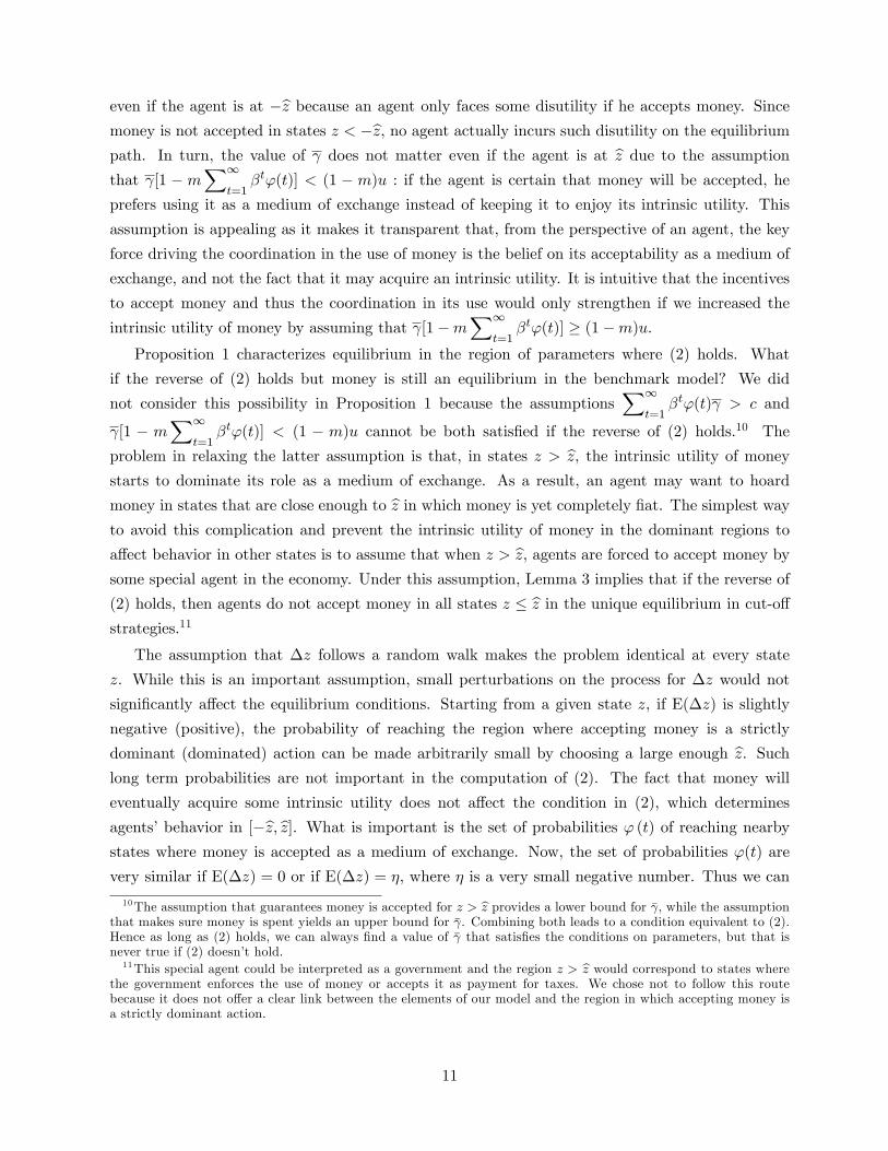
To better understand the role of �, it is useful to rewrite (2) as

�� [(1�m)u+mc] > c, (8)

where

� =

1Xt=1

�t�1' (t) . (9)

We can decompose the overall impact of an increase in � on the existence of the monetary

equilibrium into two separate e¤ects: an e¢ ciency e¤ect and a coordination e¤ect. The e¢ ciency

e¤ect takes as given the belief that money is accepted by all the other agents, and considers how

an increase in � a¤ects the incentives of an agent to produce in exchange for money. The intuition

underlying this e¤ect is straightforward: since money acquired today only commands value in the

future, an increase in � implies a larger gain from trade, thus increasing the incentives of a single

agent to accept money.

The e¢ ciency e¤ect is not novel and is present in any model of money that separates between the

act of producing in exchange for money and the act of consuming with money previously acquired.

However, since models of money take as given the belief that money is accepted as a medium of

13Alternatively, we could consider a setting in which � is �xed, but agents are randomly and anonymously matchedin pairs n � 1 times in each period. An increase in n would then amount to an increase in the arrival rate oftrading opportunities. We obtain the same results with this alternative speci�cation, but since the agent�s decisionon whether to accept money depends on the state of the economy, when there is more than one meeting in a period,we need to assume that the state of the economy changes across meetings and not across periods. This way, if � isthe period discount factor and there are n meetings in a period, then �

1n is the discount factor in between meetings.

The analysis then is exactly the same as in section 2.3, with �1n replacing �. As n goes to 1, this discount factor

goes to one.

13

exchange, they do not have much to say about the coordination problem involved in the use of

money. This is where a key contribution of this paper lies. In addition to the e¢ ciency channel,

we uncover a second channel through which an increase in � impacts the existence of a monetary

equilibrium. This coordination channel considers how an increase in � a¤ects the beliefs of agents

about the acceptability of money in states where money has no intrinsic utility.

In order to better understand the coordination e¤ect, remember that the left-hand side of (8)

corresponds to the net bene�t of having money at the end of the period in some state z 2 [�bz; bz],if the agent holds the belief that money is accepted if and only if z0 � z. In proposition 1 , we haveshown that if the net bene�t of holding money under the cut-o¤ belief is larger than the production

cost c, then money is accepted in all states where it has no intrinsic utility. Since the value of �

in (9) strictly increases with �, a larger � facilitates the coordination in the use of money. The

intuition runs as follows. If an agent expects to meet many partners in a short period of time, he

is willing to accept money even if he believes that a large number of his future partners will not

accept money. That a¤ects beliefs of all other agents: they know others will be willing to produce

in exchange for money, even if they hold relatively pessimistic beliefs. Consequently, pessimistic

beliefs cannot be an equilibrium.

It is instructive to think of an economy where one agent has a di¤erent and, say, low time

discount factor �call it �L < �. Whether money will be accepted in [�bz; bz] depends on whether (2)holds: it is the other agents�s � that a¤ects the coordination channel. If (2) holds, the impacient

agent will also accept money in states far enough from either dominant region as long as his impa-

tience is not large enough to eliminate his gains from trade (i.e., as long as �L [(1�m)u+mc] > c).We can isolate the e¢ ciency e¤ect by �xing � and looking at how changes in � a¤ect the left-

hand side of (8). In turn, we can isolate the coordination e¤ect by �xing � in (8) and looking at

how changes in � a¤ect the value of � in (9), and how changes in � a¤ect the left-hand side of (8).

We obtain

@��

@�=

8>>>><>>>>:1Xt=1

�t�1' (t)| {z }e¢ ciency e¤ect

+1Xt=1

(t� 1)�t�1' (t)| {z }coordination e¤ect

9>>>>=>>>>; .Both the e¢ ciency and the coordination e¤ects are positive and increasing in �. Moreover, as �

increases, the role of the coordination e¤ect becomes relatively more important in explaining the

existence of the monetary equilibrium.

It is particularly interesting to look at the extreme case where � converges to one. To do

so, consider �rst the scenario where the stochastic process that governs �z is symmetric, that is,

E(�z) = 0. In this case, since the probability that the economy will eventually reach a state to the

right of the current state is equal to one (that is,P1t=1 � (t) = 1) it must be that � converges to one

as � converges to one. This means that if one restricts attention to the region of parameters where

money is an equilibrium in the benchmark model of section 2.2, then if � = 1, money is always the

14

Figure 1: Normal case

unique equilibrium in the model of section 2.3.

It is possible to construct an example where the probability of ever getting to the region where

holding money is a strictly dominant action is arbitrarily small and still, as � goes to 1, � converges

to one. Let E(�z) = � for some � < 0. Since �zt follows a continuous probability distribution,

as � approaches zero and � goes to one, � converges to one. Now, for any � < 0 there exists

a large enough bz so that the probability of ever reaching states z > bz is arbitrarily small, andthe probability of reaching states z < �bz is equal to one. Therefore, as � goes to one, moneyis the unique equilibrium in the general model in the region where it is an equilibrium in the

benchmark model, despite the probability that money will ever acquire a positive intrinsic utility

being arbitrarily small and the probability that it will eventually acquire a negative intrinsic utility

being equal to one. A larger � helps agents to coordinate in the monetary equilibrium even if

E(�z) < 0 and the economy is bound to reach a region where accepting money is a strictly

dominated action.

An inspection of the expression in (9) shows that � is increasing and convex in �. In the case

E(�z) = 0, we also observe that � = 1=2 as � approaches 0. As an example, Figure 1 shows how �

varies with � for a normal process assuming E(�z) = 0. The probabilities ' (t) are obtained from

Monte Carlo simulations (they do not depend on the variance Var(z)).

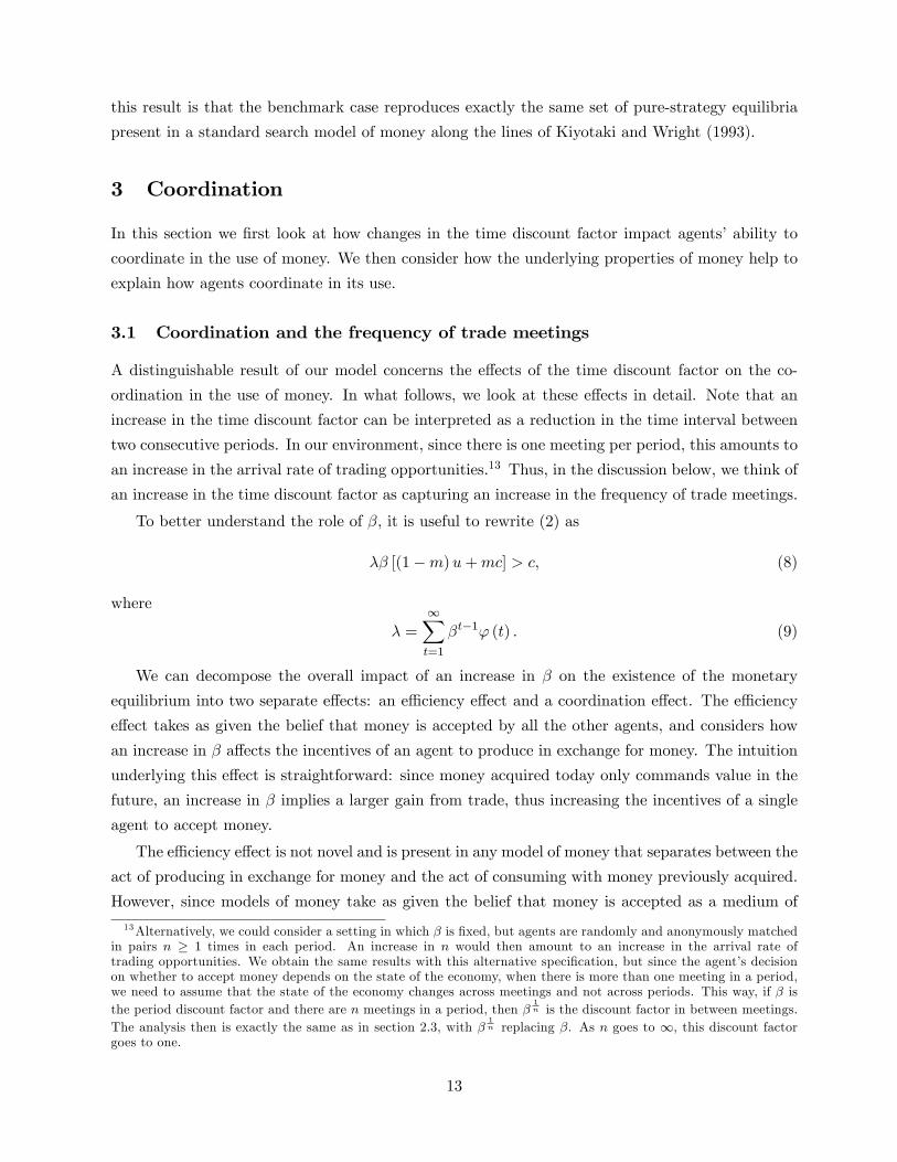
The conditions for existence of the monetary equilibrium in the benchmark model and in the

general model depend on �,m, u and c. Normalizing c = 1 and assumingm = 1=2, which maximizes

the number of trade meetings, the possible equilibria are drawn in Figure 2. Above the solid curve,

both money and autarky are equilibria in the benchmark model. Above the dotted line, money

is accepted in all states z 2 [�bz; bz] in the unique equilibrium of the general model. The distance

15

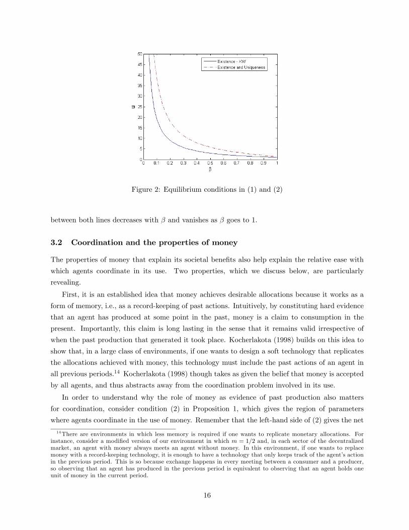
Figure 2: Equilibrium conditions in (1) and (2)

between both lines decreases with � and vanishes as � goes to 1.

3.2 Coordination and the properties of money

The properties of money that explain its societal bene�ts also help explain the relative ease with

which agents coordinate in its use. Two properties, which we discuss below, are particularly

revealing.

First, it is an established idea that money achieves desirable allocations because it works as a

form of memory, i.e., as a record-keeping of past actions. Intuitively, by constituting hard evidence

that an agent has produced at some point in the past, money is a claim to consumption in the

present. Importantly, this claim is long lasting in the sense that it remains valid irrespective of

when the past production that generated it took place. Kocherlakota (1998) builds on this idea to

show that, in a large class of environments, if one wants to design a soft technology that replicates

the allocations achieved with money, this technology must include the past actions of an agent in

all previous periods.14 Kocherlakota (1998) though takes as given the belief that money is accepted

by all agents, and thus abstracts away from the coordination problem involved in its use.

In order to understand why the role of money as evidence of past production also matters

for coordination, consider condition (2) in Proposition 1, which gives the region of parameters

where agents coordinate in the use of money. Remember that the left-hand side of (2) gives the net

14There are environments in which less memory is required if one wants to replicate monetary allocations. Forinstance, consider a modi�ed version of our environment in which m = 1=2 and, in each sector of the decentralizedmarket, an agent with money always meets an agent without money. In this environment, if one wants to replacemoney with a record-keeping technology, it is enough to have a technology that only keeps track of the agent�s actionin the previous period. This is so because exchange happens in every meeting between a consumer and a producer,so observing that an agent has produced in the previous period is equivalent to observing that an agent holds oneunit of money in the current period.

16

expected payo¤ of producing in exchange for money under the belief that all the other agents follow

a cut-o¤ strategy at the current state of the economy. This region implicitly assumes that money

perfectly records the fact that, at some point in the past, an agent produced to another agent

who liked his good. This is so because it may take many periods until an agent reaches a state at

which money is accepted, i.e., a state to the right of the current state of the economy. Thus if one

wants to design a record-keeping technology that includes all the information that allows agents to

coordinate in the use of money in the region given by (2), then this technology must include the

past actions of an agent in all previous periods. Summing up, the role of money as memory not

only helps it achieve desirable allocations, as shown by Kocherlakota (1998), but also helps agents

to coordinate in its use.15

The second property of money that matters for coordination is its role as a medium of exchange.

To understand why this is important, it is instructive to draw a parallel between the coordination

problem involved in the use of money, and the coordination problem present in other settings.

First, an important element of a monetary economy is the fact that the bene�t of exerting e¤ort

in exchange for money depends not on whether agents accept money today, but on whether agents

accept money in the future. This prevents the sort of multiplicity of equilibria that arises in settings

where the decision to exert e¤ort depends on the current decisions of the other agents. Second,

and more importantly, the decision to accept money is not made once but many times, thus the

sooner the agent accepts and uses money, the sooner he will be able to accept and use it again.

To illustrate this e¤ect, consider a modi�ed version of the environment in section 2.1, in which an

agent leaves the economy after spending money for the �rst time. In order to keep the environment

stationary, assume that, after leaving the economy, the agent is replaced by a new agent with zero

units of money. This implies that

V1;z0 = m�Ez0V1 + (1�m)u,

while V0;z0 is as in (6). Thus, we obtain

V1;z0 � V0;z0 = (1�m)u+mc� (1�m)�Ez0V0.

As compared to the case where money can be accepted and spent many times, V1;z0 � V0;z0 is nowreduced by the term (1 � m)�Ez0V0. This implies that the incentives of an agent to produce inexchange for money are weaker when money can only be accepted and spent once, and especially

so if � is large. In particular, due to the presence of (1 �m)�Ez0V0 in the expression above, it isnot the case anymore that, as the discount factor goes to one, the condition for the existence of the

monetary equilibrium becomes u > c, so that agents always coordinate in the use of money. Thus,

the fact that the agent can accept and use money many times helps to coordinate in its use.

15What is important for coordination is not only that an agent meets a producer of the good he likes, but also thatthe producer is willing to accept money. Hence even though much less memory may be required in some settings toreplicate the bene�ts of money (see footnote 14 for an example), in�nite memory is always required to ensure thatagents coordinate in the use of money in the region given by (2).

17

4 Final remarks

The notion of essentiality, by emphasizing that the societal bene�ts of money come from the fact

that it achieves desirable allocations, helps identify models in which the use of money is justi�ed on

grounds of e¢ ciency (Wallace (2001)). However, it does not say much about how agents actually

end up coordinating in the use of money, and how do the primitives of the environment and the

underlying properties of money impact such coordination. We think of our paper as an initial step

in this direction.

We have chosen to present our analysis in a search model of money along the lines of Kiyotaki

and Wright (1993), a choice that is mainly driven by tractability reasons. This choice though comes

at a cost as their environment is special in some dimensions, particularly the indivisibility of money

and the indivisibility of goods �assumptions that have been relaxed in subsequent papers such as

Trejos and Wright (1995), Shi (1995, 1997) and Lagos and Wright (2005). We leave the extension to

these settings for future work. Since the environment in Kiyotaki and Wright (1993) combines key

elements that matter for the problem of coordinating in the use of money in a tractable manner,

we see it as a natural starting point.

Our results highlight that an important primitive that impacts the coordination in the use of

money is the rate at which trade meetings take place. In particular, as long as exchange is e¢ cient,

i.e., the utility of consumption is larger then the cost of production, agents always coordinate in the

use of money if the frequency of trade meetings is large enough. This is so even if the probability

that money will eventually acquire a positive intrinsic utility is arbitrarily small and the probability

that it will eventually acquire a negative intrinsic utility is equal to one. Even though the existence

of dominant regions is necessary to rule out equilibria that are insensitive to fundamentals, the

result that agents are likely to coordinate in the use of money is not driven by expectations of

enjoying its intrinsic utility in some states. The underlying properties of money, particularly the

fact that agents accept and use it many times, and the fact that money is a resilient record-keeping

technology, help explain the relative ease with which agents coordinate in its use, as compared to

other settings where coordination matters.

References

[1] Brock, W. and Scheinkman, J., 1980, Some Remarks on Monetary Policy in an Overlapping

Generations Model, in Models of Monetary Economies, edited by John Kareken and Neil

Wallace, Federal Reserve Bank of Minneapolis, Minneapolis.

[2] Burdzy, K., Frankel, D., and Pauzner A., 2001, Fast Equilibrium Selection by Rational Players

Living in a Changing World, Econometrica 68, 163-190.

18

[3] Frankel, D. and Pauzner, A., 2000, Resolving indeterminacy in dynamic settings: the role of

shocks, Quarterly Journal of Economics 115, 283-304.

[4] Kiyotaki, N. and R. Wright, 1989, On Money as a Medium of Exchange, Journal of Political

Economy 97, 927-954.

[5] Kiyotaki, N. and R. Wright, 1993, A Search-Theoretic Approach to Monetary Economics,

American Economic Review 83, 63-77.

[6] Kocherlakota, N., 1998, Money is Memory, Journal of Economic Theory, 81, 232-51.

[7] Lagos, R. and Wright, R., 2005, A Uni�ed Framework for Monetary Theory and Policy Analy-

sis, Journal of Political Economy 113, 463-484.

[8] Morris, S. and Shin, H., 2003, Global games: theory and applications, in Advances in Eco-

nomics and Econometrics (Proceedings of the Eighth World Congress of the Econometric So-

ciety), edited by M. Dewatripont, L. Hansen and S. Turnovsky; Cambridge University Press.

[9] Scheinkman, J., 1980, Discussion, in Models of Monetary Economies, edited by John Kareken

and Neil Wallace, Federal Reserve Bank of Minneapolis, Minneapolis.

[10] Shi, S., 1995, Money and Prices: A Model of Search and Bargaining, Journal of Economic

Theory, 67, 467-496.

[11] Shi, S., 1997, A Divisible Search Model of Fiat Money, Econometrica 65, 75-102.

[12] Trejos, A. Wright, R., 1995, Search, Bargaining, Money, and Prices, Journal of Political Econ-

omy 103, 118-141.

[13] Wallace, N., 2001, Whither Monetary Economics?, International Economic Review, 42:4, 847-

869.

[14] Wallace, N. and T. Zhu, 2004, A Commodity-Money Re�nement in Matching Models, Journal

of Economic Theory 117, 246-258

[15] Zhou, R., 2003, Does Commodity Money Eliminate the Indeterminacy of Equilibria?, Journal

of Economic Theory 110, 176�190.

[16] Zhu, T., 2003, Existence of a Monetary Steady State in a Matching Model: Indivisible Money,

Journal of Economic Theory 112, 307-324.

[17] Zhu, T., 2005, Existence of a Monetary Steady State in a Matching Model: Divisible Money,

Journal of Economic Theory 123, 135-160.

19

A Proofs

Proof of Lemma 1 First, note that, if all the other agents are following a cut-o¤ strategy at z�,

then the optimal strategy only depends on the current state of the economy, i.e., it does not depend

on the particular history of realizations that led up to that state. This is so because �zt follows

a continuous probability distribution that is independent of the current and the past states of the

economy. Let then �� (z�) denote the optimal strategy of an agent given that all other agents are

following a cut-o¤ strategy at z�. If the current state is z and the agent follows the optimal strategy,

we let the expected payo¤ of holding one unit of money at the end of the period be given v1(z; z�),

and the expected payo¤of holding zero units of money at the end of the period be given by v0(z; z�).

The optimal strategy can thus be described by the set Z� = fz 2 Rj � c+ v1(z; z�) > v0(z; z�)g, i.e.,the set of all states in which it is optimal to accept money. If we let �v(z; z�) = v1(z; z�)�v0(z; z�),our objective is to prove that �v(z; z�) is strictly increasing in z.

In what follows, we will �rst ignore the intrinsic utility or disutility of money by assumingbz = 1. We will return to this point at the end. Let z0 be the state of the economy in period 1and let �w (z�) be the following (potentially sub-optimal) strategy: (1) accept money in state z0 if

and only if z0 + w 2 Z�, where w > 0, (2) if the agent participated in a meeting in which moneywas acceptable by at least one agent in a previous period, then follow the optimal strategy from

that period on, (3) if the agent did not participate in a meeting where money was acceptable by at

least one agent in a previous period, then accept money if and only if either z0 + w +�z1 2 Z� orz0+w+�z1 > z�, where �z1 is the realization of the stochastic process in period 1, (4) if the agent

did not participate in a meeting where money was acceptable by at least one agent in a previous

period, and it was not the case that z0 + w + �z1 2 Z� or z0 + w + �z1 > z�, then behave as in(3) replacing z0 +w+�z1 with z0 +w+�z1 +�z2, where �z2 is the realization of the stochastic

process in period 2. This process continues until a period is reached where the agent participates

in a meeting where money is acceptable by at least one of the agents in the meeting, in which case

the agent follows the optimal strategy from that period on.

Note that, if the agent following �w (z�) accepts money in a given period, his expected payo¤

in state z is given by �c+ v1(z; z�). Indeed, the agent follows the optimal strategy after acceptingmoney. Let then Vn(z; z�) be the expected payo¤ of not accepting money in state z if the agent

follows the strategy �w (z�). De�ne �V (z0; z�) = v1(z0; z�) � Vn(z0; z�). Since �w (z�) is not

necessarily the optimal strategy, Vn(z0; z�) � v0(z0; z�). Hence �V (z0; z�) > �v(z0; z�). If we provethat �v(z0 + w; z�) > �V (z0; z�), then it must be that �v(z0 + w; z�) > �v(z0; z�), in which case

v1(z; z�)� v0(z; z�) is strictly increasing in z.

In order to prove that �v(z0+w; z�) > �V (z0; z�), we compare payo¤s from an agent starting at

z0 following the strategy �w (z�) and another agent starting at z0+w following the optimal strategy

�� (z�), for any given realization of the random process �z. There are six cases that we need to

consider. Henceforth, let DV (�z) denote the di¤erence between the net bene�t of carrying money

20

if the current state is z0 + w +�z and the agent follows the optimal strategy, and the net bene�t

of carrying money if the current state is z0 +�z and the agent follows �w (z�).

The �rst possibility is that z0 + �z > z� and z0 + w + �z 2 Z�. In this case, it is optimal toaccept money if the current state is z0 + w + �z (hence, money is accepted under �w (z�)), and

money is accepted by all other agents if the current state is either z0 + �z or z0 + w + �z. This

implies that DV (�z) = 0.

The second possibility is that z0 +�z < z� < z0 + w +�z and z0 + w +�z 2 Z�. In this case,it is optimal to accept money if the current state is z0 + w + �z, money is accepted by all other

agents if the state is z0 +w+�z, but is is not accepted by the other agents if the state is z0 +�z.

This implies that

DV (�z) = (1�m) [u� �Ez0+�z(v1 � v0)] ,

where Ez0+�z(v1 � v0) is the net continuation payo¤ of having money when the current state isz0 +�z and the agent follows the optimal strategy.

The third possibility is that z0 +w+�z < z� and z0 +w+�z 2 Z�. In this case, it is optimalto accept money if the current state is z0 +w +�z, but money is not accepted by all other agents

if the current state is either z0 + w +�z or z0 +�z. This implies that

DV (�z) = (1�m)� [Ez0+w+�z(v1 � v0)� Ez0+�z(v1 � v0)] .

The fourth possibility is that z0+�z > z� and z0+w+�z =2 Z�. In this case, it is not optimalto accept money if the current state is z0 + w +�z (hence, money is not accepted under �w (z�)),

and money is accepted by all other agents if the current state is either z00 + �z or z0 + �z. This

implies that

DV (�z) = m� [Ez0+w+�z(v1 � v0)� Ez0+�z(v1 � v0)] .

The �fth possibility is that z0 +�z < z� < z0 + w +�z and z0 + w +�z =2 Z�. In this case, itis not optimal to accept money if the current state is z0 + w +�z, money is accepted by all other

agents if the current state is z0 + w +�z, but it is not accepted by the other agents if the current

state is z0 +�z. This implies that

DV (�z) = (1�m) [u� �Ez0+�z(v1 � v0)] +m� [Ez0+w+�z(v1 � v0)� Ez0+�z(v1 � v0)] .

Finally, the last possibility is that z0 + w + �z < z� and z0 + w + �z =2 Z�. In this case,irrespective of whether the current state is z0 + w +�z or z0 +�z, money is not accepted by the

agent and by all other agents. Thus

DV (�z) = � [Ez0+w+�z(v1 � v0)� Ez0+�z(v1 � v0)] .

Now, note that in all possibilities considered above, it is never the case that the agent following

�z0 in state z0 + �z obtains a higher �ow payo¤ than the agent following the optimal strategy in

state z0 + w + �z. Indeed, in the �rst, third, fourth and sixth possibilities, the �ow payo¤ is the

21

same for both agents. In turn, in the second and the �fth possibilities, the agent that follows the

optimal strategy obtains a strictly higher �ow payo¤. This is so because Ez0+�z(v1�v0) is boundedabove by u. Now, since the agent�s expected payo¤ is the expected sum of the �ow payo¤s he will

obtain in the current and in all future periods, it must be the case thatZ�zDV (�z)f(�z)d�z > 0.

This proves that �v(z0 + w; z�) > �V (z0; z�), and so �v(z0 + w; z�) > �v(z0; z�). Since w > 0 is

generic, we obtain that v1(z; z�) � v0(z; z�) is strictly increasing in z. This implies that the bestresponse to all the other agents following a cut-o¤ strategy at z�, is to also follow a cut-o¤ strategy.

It also implies the the best response is unique, in which case we can denote it by the cut-o¤ state

Z1(z�).

Now, let�s consider the case with a �nite bz. As long as Z1(z�) 2 [�bz; bz], nothing changesin the proof, because the utility (or disutility) (z) has no e¤ect on the optimal strategy in the

dominant regions (the agent �nds it optimal to accept money if z > bz and not to accept moneyif z < �bz) and for a small enough w, the agent following the strategy �w (z�) is never forced toaccept money for some z < �bz. The cut-o¤ strategy for a �nite bz is not a¤ected by the dominantregions, Z(z�) = Z1(z�).

If Z1(z�) > bz, the proof is not a¤ected. If v1(z; z�) � v0(z; z�) happens to be positive for allvalues of z, then Z(z�) = bz, and money is never accepted in the interesting region. Things aredi¤erent in case Z1(z�) < �bz. The proof cannot be adapted to cover this case because the agentfollowing the strategy �w (z�) would be forced to accept money, and thus face the disutility cost

(z), in some states in which money has a negative intrinsic utility. Now, we know that ignoring

the dominant regions, Z1(z�) < �bz implies that v1(z; z�) � v0(z; z�) > 0 for all z 2 [�bz; bz]. Wecan show that once we impose that the agent cannot choose to make an e¤ort in a set of arbitrary

states, the di¤erence v1(z; z�) � v0(z; z�) can only increase. The argument runs as follows. Thedi¤erence v1(z; z�)� v0(z; z�) is given by

1Xt=0

�1(t)c��1 + �t

�+

1Xt=0

�2(t)�t [(1�m)u+mc]

where �1(t) is the probability that an agent that has not accepted money at state z will accept

money after t periods before the economy reaches a state z > z�, and �2(t) is the probability that

the economy will reach a state z > z� before the agent that has not accepted money at state z

will get another opportunity to accept money. The term multiplying �1(t) is the cost of incurring

the cost c at the current period instead of doing so after t periods. The term multiplying �2(t) is

the di¤erence of the value of reaching a state z > z� with and without money �the argument here

is the same as the one that leads to (7). Taking the option of accepting money of an agent in a

later period can only decrease �1(t) and increase �2(t), which can only increase v1(z; z�)�v0(z; z�).

Hence Z1(z�) < �bz implies that the agent follows a cut-o¤ strategy around the state Z(z�) = �bz.22

Proof of Lemma 2 We want to show that, if an agent is following a cut-o¤ strategy at z 2 [�bz; bz]and all the other agents are following a cut-o¤ strategy at z0 2 [�bz; bz], then the net expected payo¤of producing in exchange for money in state z is strictly decreasing in z0.

Consider, �rst, the scenario where z0 < z. There are three possibilities that we need to consider,

depending on the realization of the random process �z. The �rst possibility is that z +�z < z0.

In this case, money is not accepted by the agent and is not accepted by all the other agents. Thus,

the net expected payo¤ of having one unit of money is given by

�Ez+�z[V1(z +�z; z0; z)� V0(z +�z; z0; z)].

The second possibility is that z +�z 2 [z0; z). In this case, the agent does not accept money butall the other agents do so. Thus, the net expected payo¤ of having one unit of money is given by

(1�m)u+m�Ez+�z[V1(z +�z; z0; z)� V0(z +�z; z0; z)].

Finally, the last possibility is that z+�z � z. In this case, money is always accepted, and the netexpected payo¤ of having one unit of money is

(1�m)u+mc.

Note that, whenever z0 < z, the probability of the last possibility is independent of z0. Now, since

(i) the net expected payo¤ under the second possibility is higher than that of the �rst possibility,

and (ii) the probability of the second possibility is strictly decreasing in z0, it must be the case that

the net bene�t of producing in exchange for money in state z is strictly decreasing in z0, for all

z0 < z.

Consider, now, the scenario where z0 > z. Again, there are three possibilities that we need

to consider, depending on the realization of the random process �z. The �rst possibility is that

z +�z < z. In this case, since money is not accepted by the agent and is not accepted by all the

other agents, the net expected payo¤ of having one unit of money is given by

�Ez+�z[V1(z +�z; z0; z)� V0(z +�z; z0; z)].

The second possibility is that z + �z 2 [z; z0). In this case, the agent accepts money but all theother agents do not do so. As a result, the net expected payo¤ of having one unit of money is given

by

(1�m)�Ez+�z[V1(z +�z; z0; z)� V0(z +�z; z0; z)] +mc.

The third possibility is that z + �z � z0. In this case, money is always accepted, and the net

expected payo¤ of having one unit of money is

(1�m)u+mc.

Note that, whenever z0 > z, the probability of the �rst possibility is independent of z0. Now,

since (i) the net expected payo¤ under the second possibility is strictly lower than that of the

23

third possibility (�Ez+�z[V1(z +�z; z0; z)� V0(z +�z; z0; z)] is bounded above by u), and (ii) theprobability of the second possibility is strictly increasing in z0, it must be the case that the net

bene�t of producing in exchange for money in state z is strictly decreasing in z0, for all z0 > z.

Proof of Lemma 3 First, since the random process �zt follows a continuous probability distri-

bution that is independent of the current state z, it must be that for all z and z0 in [�bz; bz],V1(z; z; z)� V0(z; z; z) = V1(z0; z0; z0)� V0(z0; z0; z0). (10)

Now, there exists a unique Z(z) that is a best response to all agents following a cut-o¤ strategy at

z (Lemma 1). By de�nition, Z(z) satis�es

� fV1 [Z(z); z; Z(z)]� V0 [Z(z); z; Z(z)]g = c.

Let z 2 (�bz; bz) and assume that� [V1(z; z; z)� V0(z; z; z)] > c. (11)

This implies

�c+ � fV1 [Z(z); z; Z(z)]� V0 [Z(z); z; Z(z)]g < �c+ � [V1(z; z; z)� V0(z; z; z)] ,

that is,

V1 [Z(z); z; Z(z)]� V0 [Z(z); z; Z(z)] < V1(z; z; z)� V0(z; z; z). (12)

Given (10), we can rewrite (12) as

V1 [Z(z); z; Z(z)]� V0 [Z(z); z; Z(z)] < V1 [Z(z); Z(z); Z(z)]� V0 [Z(z); Z(z); Z(z)] .

Since V1 [Z(z); z; Z(z)] � V0 [Z(z); z; Z(z)] is strictly decreasing in z (Lemma 2), it must be thatZ(z) < z. This implies that it is strictly optimal to accept money in state z. Since this reasoning

holds for all z 2 (�bz; bz), a continuity argument implies that is it also optimal to accept money instate �bz.

Now let z 2 (�bz; bz) and assume that� [V1(z; z; z)� V0(z; z; z)] < c. (13)

This implies

�c+ � fV1 [Z(z); z; Z(z)]� V0 [Z(z); z; Z(z)]g > �c+ � [V1(z; z; z)� V0(z; z; z)] ,

that is,

V1 [Z(z); z; Z(z)]� V0 [Z(z); z; Z(z)] > V1(z; z; z)� V0(z; z; z). (14)

24

Again, given (10), we can rewrite (14) as

V1 [Z(z); z; Z(z)]� V0 [Z(z); z; Z(z)] > V1 [Z(z); Z(z); Z(z)]� V0 [Z(z); Z(z); Z(z)] .

Since V1 [Z(z); z; Z(z)]�V0 [Z(z); z; Z(z)] is strictly decreasing in z, it must be that Z(z) > z. Thisimplies that it is strictly optimal not to accept money in state z. Since this reasoning holds for all

z 2 (�bz; bz), a continuity argument implies that is it also optimal not to accept money in state bz.Proof of Lemma 4 Suppose an equilibrium where agents follow di¤erent thresholds z�i 2 [�z; z].Consider the highest and smallest thresholds, z�H and z�L respectively. Since agents have to be

indi¤erent at those thresholds, we have

�c+ �V1(z�H ; z�H)� �V0(z�H ; z�H) = 0 = �c+ �V1(z�L; z�L)� �V0(z�L; z�L) (15)

where Vi(z0; z0) is the relative payo¤ of �nishing the period with i units of money at state z0,

following a cut-o¤ strategy at state z0. Now note that at the left of z�H , money is accepted with

probability 1, while at the right of z�H , money is accepted with some probability between 0 and 1.

Likewise, at the right of z�L, money is accepted with probability 0, while at the right of z�L, money

is accepted with some probability between 0 and 1.

Now consider an agent at z�H following a cut-o¤ strategy at z�H and an agent at z�L following

a cut-o¤ strategy at z�L. Suppose the realization of �z is positive. Then, both agents are willing

to accept money. With some probability, both would be able to spend money in which case the

di¤erence between having and not having money is worth

(1�m)u+mc

but with some probability only the agent that started at z�H is able to spend money, in which case

the di¤erence between having money or not for this agent is still (1�m)u+mc, but the di¤erencebetween having money or not for the agent that started at z�L is worth

(1�m)�Ez (V1 � V0) +mc < (1�m)u+mc

Now suppose the realization of �z is negative. Then they are not willing to accept money. With

some probability, the agent starting at z�H is able to spend money, in which case the di¤erence

between the value having money or not for him is

(1�m)u+m�Ez(V1 � V0)

but for the agent starting at z�L, the relative value of having money is

�Ez(V1 � V0)

With some probability, nobody will be able to either accept or spend money, so the relative value of

having money will be � times the value they will get in the following period. In all cases, whenever

agents realize di¤erent payo¤s, the relative value of having money for the agent at z�H is larger than

the value for the agent at z�L, which means (15) cannot hold.

25

B The case of a discrete state space

In what follows we consider the case in which the state space is discrete, given by Z, and therandom process �zt follows a discrete probability distribution that is independent of z and t, with

expected value E(�z) � 0 and variance Var(�z) > 0. In order to consider in a tractable mannerboth the region of parameters where agents coordinate in the use of money and the region where

agents do not coordinate in the use of money, we simplify the the description of the environment

by assuming that, in states z > bz, it is strictly optimal to accept money because a special agent inthe economy forces other agents to do so.

First, it is straightforward to adapt the proofs of Lemmas 1 and 2 to the discrete case. Thus, as

in Lemma 1, if all the other agents are following a cut-o¤ strategy at some state z 2 Z\ [�bz; bz], inwhich money is accepted in state z0 2 Z\[�bz; bz] if and only if z0 � z, then there exists a unique bestreply, given by the cut-o¤ strategy Z(z) 2 Z \ [�bz; bz]. Moreover, as in Lemma 2, the net bene�tof following a cut-o¤ strategy at some state z 2 Z\ [�bz; bz] is strictly decreasing in z0 2 Z\ [�bz; bz],where z0 denotes the cut-o¤ strategy followed by all the other agents. Combining Lemmas 1 and

2, it is also straightforward to show that Lemma 3 still holds, that is, in order to assess the agent�s

optimal behavior in some state z 2 Z \ [�bz; bz], it is su¢ cient to consider the payo¤s induced by asymmetric strategy pro�le where all agents choose the same cut-o¤ strategy z.

The only di¤erence in the case of a discrete state space rests in the implications of Lemma 3.

The reasoning runs as follows. As in the case of a continuous state space, since the random process

�zt follows a probability distribution that is independent of the current state z, it must be that

for all z and z0 in [�bz; bz],V1(z; z; z)� V0(z; z; z) = V1(z0; z0; z0)� V0(z0; z0; z0).

First, assume that � [V1(z; z; z)� V0(z; z; z)] > c. There exists a unique Z(z) that is a best

response to all the other agents following a cut-o¤ strategy at z (adaptation of Lemma 1). By

de�nition, Z(z) is the smallest z 2 Z \ [�bz; bz] such that� fV1 [Z(z); z; Z(z)]� V0 [Z(z); z; Z(z)]g � c.

Since V1 [Z(z); z; Z(z)]�V0 [Z(z); z; Z(z)] is strictly decreasing in z (adaptation of Lemma 2), thereare two possibilities: either Z(z) = z or Z(z) < z. In the latter case, the same reasoning applied

to the continuous state space implies that the unique symmetric equilibrium in cut-o¤ strategies is

the one in which all agents follow a cut-o¤ strategy at z = �bz. If, instead, Z(z) = z, then thereexists a symmetric equilibrium in which all agents follow a cut-o¤ strategy at z. Now, since z is

generic, then there exists one such equilibrium for each z 2 Z \ [�bz; bz].In order to pin down the whole region of parameters in which the unique equilibrium has money

always accepted in the region z 2 Z \ [�bz; bz], we only need to consider the problem of an agent in

state z � 1 2 Z \ [�bz; bz], who follows a cut-o¤ strategy at this state and believes that all the other26

agents are following a cut-o¤ strategy at state z 2 Z\ [�bz; bz]. This agent has an strict incentive toproduce in exchange for money if and only if

� [V1(z � 1; z; z � 1)� V0(z � 1; z; z � 1)] > c.

Denote by �(t) the probability of reaching any state strictly larger than z� 1 at time s+ t and notbefore. Then, we can rewrite the above condition as 1X

t=1

�t� (t)

![(1�m)u+mc] > c. (16)

Now, assume that � [V1(z; z; z)� V0(z; z; z)] < c. Again, there exists a unique Z(z) that is a

best response to all the other agents following a cut-o¤ strategy at z. By de�nition, Z(z) is the

largest z 2 Z \ [�bz; bz] such that� fV1 [Z(z)� 1; z; Z(z)� 1]� V0 [Z(z)� 1; z; Z(z)� 1]g � c.

Since V1 [Z(z); z; Z(z)] � V0 [Z(z); z; Z(z)] is strictly decreasing in z, there are two possibilities:either Z(z) = z or Z(z) > z. In the latter case, there exists a unique symmetric equilibrium in

cut-o¤ strategies, in which all agents follow a cut-o¤ strategy at z = bz + 1. If, instead, Z(z) = z,then there exists a symmetric equilibrium in which all agents follow a cut-o¤ strategy at z + 1.

Again, since z is generic, then there exists one such equilibrium for each z 2 Z \ [�bz; bz].In order to pin down the whole region of parameters in which the unique equilibrium has money

never accepted in the region z 2 Z \ [�bz; bz], we only need to consider the problem of an agent in

state z � 1 who follows a cut-o¤ strategy at state z 2 Z \ [�bz; bz] and believes that all the otheragents are following a cut-o¤ strategy at state z�1 2 Z\ [�bz; bz]. This agent has an strict incentivenot to produce in exchange for money if and only if

� [V1(z � 1; z � 1; z)� V0(z � 1; z � 1; z)] < c.

Denote by �+(t) the probability of reaching any state larger or equal than z � 1 at time s+ t andnot before. Then, we can rewrite the above condition as 1X

t=1

�t�+ (t)

![(1�m)u+mc] < c. (17)

Equations (16) or (17) are versions of (2) with �(t) or �+(t) instead of ' (t). In the continuous

case we consider the probabilities of reaching z when the economy starts in a state that is arbitrarily

close to z. Here, we have to start from the closest state where money is not accepted or the closest

state where money is accepted, depending on which strategies we want to eliminate. As there

is some distance between them, the probabilities � (t) and �+ (t) will not be the same. Hence

there will be a region with multiple equilibria. But as the support of �z increases, the discrete

27

distribution gets closer to a continuous distribution, and � (t) and �+ (t) get closer and closer to

each other.

As in the continuous case, we can rewrite condition (16) as

�M� [(1�m)u+mc] > c,

and condition (17) as

�A� [(1�m)u+mc] < c,

where

�M =

1Xt=1

�t�1� (t) and �A =

1Xt=1

�t�1�+ (t) (18)

The benchmark case corresponds to �M = 0, which means autarky is always an equilibrium, and

�A = 1, which means money is an equilibrium as long as it is an equilibrium in the benchmark model.

Clearly, (18) shows that �M and �A are increasing in �. Moreover, If E(�z) = 0,P1t=1 �+ (t) = 1

andP1t=1 � (t) = 1, thus as � ! 1, �A ! 1 and �M ! 1. That is, as the frequency of trade

meetings goes to in�nity, agents always coordinate in the use of money.

B.1 Example: Binary case

Consider a simple stochastic process where Pr(�z = 1) = p and Pr(�z = �1) = 1� p. Departingfrom state z� � 1 in period s, the probability of reaching state z� in period s+ 1 is p. Otherwise,the economy moves to state z� � 2. Then, state z� can only be reached in period s + 3. Theprobabilities that state z� will be reached for the �rst time at time s+ t are given by (for all i � 0)

�(2i+ 1) =(2i)!

i! (i+ 1)!pi+1(1� p)i and �(2i) = 0.

Remember that �(t) is the probability of reaching for the �rst time state z� at time s+ t, when the

initial state is z� � 1. The formula for �(2i + 1) resembles a binomial distribution, but the usualcombination is replaced with the Catalan numbers.16 The value of �M is given by

�M =

1Xi=0

�(2i)�

(2n)!

n! (n+ 1)!pi+1(1� p)i

�. (19)

Departing from state z� in period s, the probability of reaching a state larger than z� in period

s + 1 is p. Otherwise, the economy moves to state z� � 1, which happens with probability 1 � p.At z� � 1, we are at the previous case. Thus (for all i � 0)

�+(1) = p,

�+(2i+ 2) = (1� p) (2i)!

i! (i+ 1)!pi+1(1� p)i,

�+(2i+ 3) = 0.

16See, e.g., http://mathworld.wolfram.com/CatalanNumber.html.

28

Figure 3: Binary case: �M and �A

Hence

�A = p+ (1� p)1Xi=0

�(2i+1)�

(2n)!

n! (n+ 1)!pi+1(1� p)i

��A = p+ (1� p)��M (20)

The case p = 0:5 If p = 0:5, �M becomes:

�M =

1Xi=0

�(2i)

(2i)!

i! (i+ 1)!

�1

2

�2i+1!(21)

which is a function of � only, and �A is then �A =1+��M

2 . Figure 3 shows �A and �M as a function

of �. It turns out that the factor � for a normal distributions lies between the lines for �A and �M .

The multiple-equilibrium region is larger for intermediate values of �, and vanishes as � approaches

1. The curves for �A and �M are similar to � in the continuous case: both �M and �A converge to

1 as � approaches 1, converge to 0.5 as � approaches 0, are increasing in � and convex.

29