F 609 Relatorio Final Pirani - ifi.unicamp.brlunazzi/F530_F590_F690_F809_F895/F809/... · O Pirani é um instrumento utilizado para medir pressão na faixa de 200 a 10-4 torr (baixo

F 609Relatorio Final

Pirani

Nome do aluno: Fabio Lofredo Cesar E-mail: [email protected] do orientador: Abner de Siervo E-mail: [email protected]

mailto:[email protected]

1)Introdução:O Pirani é um instrumento utilizado para medir pressão na faixa de 200 a 10-4

torr (baixo vácuo). O vácuo tem extrema importância em inúmeras áreas desde a pesquisa básica até processos industriais, como em refinamento e secagem de materiais e outros. A medida do vácuo produzido é importante para saber se há ou não vazamento no sistema, saber se possui vácuo suficiente para o seu objetivo como por exemplos certos equipamentos so funcionam em certas faixas de pressões muito baixas; ou ainda, garantir a qualidade nos processos utilizados.

O Pirani é um manômetro, que leva este nome em homenagem a seu inventor, Marcelo Pirani (1906). O princípio de funcionamento do Pirani é a da variação da condutividade térmica como função da pressão. Desta forma é possível medir a pressão se conhecermos a corrente que passa por um filamento aquecido.

2)TeoriaPara um filamento aquecido, os choques de moléculas de gás retiram calor do

mesmo, trocando energia térmica por energia cinética das moléculas. Quanto mais gas possuir a camera mais calor é retirado do filamento. Sabemos no entanto que a resistividade dos materiais depende da temperatura. Como o número de choques de moléculas do gás na câmara sobre o filamento depende da pressão, temos q ue a resistencia do filamento é uma função direta da pressão. Portanto, podemos utilizar um filamento, sob uma tensão constante e medir a corrente do amperimetro como função da pressão da câmara. Com isto devemos observar uma variação da resistencia do filamento como função da pressão dentro da câmara. Assim podemos, com um sistema ja calibrado, estimar a pressão dentro da camera com o amperimetro para uma escala de pressão definida.

Para pressões muito alta e muito baixas o pirani mostra perda de precisão, pois para pressões altas o ambiente ja possui muitas particulas retirando calor do filamento, se diminuir com modereção, não ira mudar efetivamente a perda de calor por convecção. No limite oposto, para pressões muito baixas, a perda de calor do filamento na forma de radiação começa a ser muito mais importante do que as perdas pelos choques, diminuindo portanto a sensibilidade e a capacidade de medição.

Como a variação da resistência na faixa de temperatura em que o filamento opera (~200C) é muito pequena, a utilização de um circuito com ponte de Wheatstone ajuda a aumentar a sensibilidade medida por um micro-amperímetro que pode ser encontrado em qualquer loja de eletroeletrônicos a preços bastante assessíveis (~R15,00).

3)Construção Conseguimos uma pequena lâmpada incandecente tipica das utilizadas em carros e motos de 12V/2W. Esta será utilizada como o nosso sensor Pirani em si e também poupará o trabalho de confeccionar passantes elétricos para vácuo. Foi furada um flange do tipo KF para encaixar o bulbo da lâmpada. Cortamos o bulbo da lâmpada, e colamos o mesmo à flange com araldite. Utilizamos araldite 24h pois ela produz menos degase do que a de secagem rápida.

Conseguimos as conexões para vacuo, flanges, tubo, bomba, válvula agulha, manômetro também do tipo Pirani (comercial e calibrado), fonte e multímetro emprestados pelo laboratório de física de superfícies do DFA. Fizemos um circuito elétrico com ponte de Wheatstone para dar mais sensibilidade a medição no amperimetro. A idéia é poder aquecer o filamento utilizando uma fonte de corrente constante.

Construimos uma pequena caixa de tubo para suportar o circuito elétrico, ele possui entrada para a fonte e para o amperimetro.

Legenda: figura mostrando a ponte de wheatstone

4)Resultados da calibração do Pirani Foi coletado dados de pressão e corrente com o medidor de pressão e o amperimetro para diversas tensões fornecidas pela fonte conforme a tabela abaixo:

E com estes dados plotamos os seguintes graficos:

Pressão (10^-6 torr) Corrente (10^-6 A)Medida Erro Para 0,5V Para 0,4V Para 0,3V Para 0,2V Para 0,1V Erro

atm 100 0 0.3 0 0.2 0.1 0.12000 100 1.4 1.2 0.4 0.3 0.1 0.11000 100 2.4 1.5 0.6 0.3 0.1 0.1750 25 3.1 2 0.7 0.4 0.1 0.1500 25 4.1 2.8 0.8 0.4 0.1 0.1400 10 4.9 3.2 1 0.5 0.2 0.1300 10 6.1 3.9 1.2 0.5 0.2 0.1250 5 6.7 4.2 1.4 0.6 0.2 0.1200 5 7.7 4.7 1.6 0.6 0.2 0.1150 5 9.9 5.7 1.9 0.7 0.2 0.1100 5 12 6.8 2.3 0.8 0.2 0.180 3 13 7.2 2.5 0.9 0.2 0.160 3 14.3 8.1 2.8 0.9 0.2 0.1

Analisando os graficos, podemos ver que a corrente é uma função da pressão, e que conforme aumentamos a tensão da fonte mais sensivel é o sistema, porem se a tensão for aumentada demasiadamente, podera queimar o filamento no regime de pressões próximo da atmosfera, simplismente pela oxidação do mesmo. No gráfico logaritmo, os dados se aproximam mais a uma reta, porem o objetivo é mostrar que pressão e a corrente variam de forma proporcional e não necessariamente linear.

5)Fotos da experiência.-Sistema completo

Legenda:

1) Fonte de tensão

2) Manômetro

3)Amperimetro (no momento encontra-se em calibração)

4)Circuito eletrico com ponte de Wheatstone em um protoboard temporario(foi substituido pela caixa de tubo, ver abaixo)

5)Sistema de vácuo (ver foto abaixo)

6)Bomba Mecânica

-Sistema de vácuo

Legenda:

1)Conexão para bomba mecanica

2)Lampada com filamento colada com araldite (ver foto abaixo)

3)Conexão para o medidor de pressão (manômetro do tipo Pirani).

4)Valvula agulha para variar a pressão

-Lampada com filamento colada com araldite

Legenda: Lampada de 12V/2W colada com araldite na flange e fios soldados para ligar ao circuito elétrico.

-Tubo de PVC para suportar o circuito elétrico

Legenda: Ttubo de PVC com o circuito eletrico do pirani.

Legenda: Tubo PVC (visão lateral) fios para ligar a fonte e o amperimetro.

6)Dificultades encontradasTentamos fazer o filamento de tungstenio, porem ia ser mais complicado e

dificil fazer o vidro, colar o vidro e sair com os filamentos para fora do vidro, para isso achamos na literatura que uma lampada normal serviria.

Para fixar o bulbo da lâmpada ao sistema de vácuo foi usinada uma flange. Usamos araldite 24hs para fixar o bulbo da lâmpada na flange, porem ela possui a desvantagem de escorrer durante o endurecimento, e isso pode não fortalecer o suficiente o bulbo fixado na flange já que o bulbo é um vidro frágil, mas o sistema parece funcionar perfeitamente. O uso de durepoxi e araldite de 90min, não foram bem sucedidos, pois eles não garantiam um bom vácuo, pois o durepoxi é poroso e araldite de 90min libera gases.

Procuramos um componente eletronico para aumentar o sinal da tensão, porem o laboratorio somente tinha um tipo de componente e ele não era adequado, pois poderia causar erros grandes na medição caso fosse fornecida uma corrente relativamente alta, ainda iremos testar para ver sua eficiencia.

Conseguimos um pequeno circuito ja usado para fazer a ponte de wheatstone, porem o circuito tinha varios caminhos quebrados, o que necessitou de algumas ligações e soldas a mais para conectar os caminhos quebrados.

A princípio, fizemos teste e o sistema parecia funcionar perfeitamente, porém a escala de pressão estava diferente da literatura, então levamos para calibar o medidor de pirâni.

Este pirani descalibra facilmente se mudado de situação o sistema, e o potenciometro é muito sensivel. O manômetro quebrou durante a utilização do sistema, porem este não teve implicações para o pirani visto que a função dele era apenas situar a pressão numa escala e não mostrar o efeito do filmento no vacuo.

7)Opinião do orientador“Meu orientador concorda com o expressado neste relatório final e deu a

seguinte opinião:

O aluno mostrou-se interessado no problema. Procurou solucinar as dificuldade por conta própria mostrando iniciativa. No entanto, acredito que o trabalho poderia ter explorado um pouco melhor outros efeitos como a variação da pressão como função do tipo de gás utilizado. Apesar de proposto inicialmente, não foi possível executar esta parte do experimento devido ao tempo. O aluno também poderia ter comparado seus resultados com aqueles encontrados na literatura existente, tornando o trabalho mais rico em detalhamento físico, inclusive com a proposição de um

modelo teórico para ajustar às curvas medidas; e assim melhor compreender o fenômeno que está sendo estudado. Apesar disto, a proposta inicial foi cumprida integralmente e os resultados esperados atingidos. Avalio que o experimento foi um sucesso.

8)Referencias:

Estão abaixo, em anexo, algumas referencias:

A wide range constant-resistance Pirani gauge with ambient temperature compensation

This article has been downloaded from IOPscience. Please scroll down to see the full text article.

1965 J. Sci. Instrum. 42 77

(http://iopscience.iop.org/0950-7671/42/2/304)

Download details:

IP Address: 143.106.72.69

The article was downloaded on 10/09/2010 at 13:03

Please note that terms and conditions apply.

View the table of contents for this issue, or go to the journal homepage for more

Home Search Collections Journals About Contact us My IOPscience

http://iopscience.iop.org/page/terms

http://iopscience.iop.org/0950-7671/42/2

http://iopscience.iop.org/0950-7671

http://iopscience.iop.org/

http://iopscience.iop.org/search

http://iopscience.iop.org/collections

http://iopscience.iop.org/journals

http://iopscience.iop.org/page/aboutioppublishing

http://iopscience.iop.org/contact

http://iopscience.iop.org/myiopscience


J. ENGLISH, B. FLETCHER and W. STECKELMACHER Central Research Laboratory, Edwards High Vacuum International Ltd., Crawley, Sussex Paper presented at the Conference on Fundamental Problems of Low Pressure Measurements, September 1964; MS. received 14th October 1964

Abstract. The development of a Pirani gauge to cover the pressure range from 10 mtorr to 200 torr is described. A thin wire filament was used in a d.c. Wheatstone bridge with a transistor d.c. amplifier automatically varying the voltage so as to maintain the filament at constant temperature. With this arrangement, the bridge voltage is a function of pressure. It was found desirable to divide the pressure range into three sections, with automatic switching from one to the other. To measure pressures above 10 torr with any confidence it is necessary to provide ambient temperature compensation. To maintain a constant temperature difference between the gauge filament and wall, a temperature- dependent resistor was wound on the tubular gauge envelope and included in the opposite arm of the Wheatstone bridge. In addition to compensating for ambient temperature variations, this resistor also corrected for heating of the envelope, by conduction from the filament, at high pressures, thereby greatly reducing the time from switching on the flament to obtain a correct reading.

1. Introduction A Pirani gauge element connected in a conventional Wheat- stone bridge circuit may be operated at a practically constant temperature by adjusting the bridge supply voltage in such a way as to keep the bridge balanced. With equal ratio arms, the resistance in the other bridge arm is a measure of the filament resistance and therefore filament temperature. The bridge voltage, adjusted at each pressure, is a measure of the energy supplied to the gauge dament. Such an arrangement was used in early studies into the thermal interaction between gases and solid surfaces at different pressures.

Although hot wire devices such as anemometers have been operated for a considerable time at constant temperature using suitable feedback circuits, it is thanks to the work of von Ubisch (1947, 1948a, b, 1951, 1952, 1957) that these methods of control have found wide use in Pirani gauges, and a number of such instruments are now available. An instrument following the original design of von Ubisch is commercially available under ?he niL?le 'Autoviic'. Ubisch (1947, 1948 a, b, 1951, 1952) investigated the effect of gauge geometry, different size filaments, on the pressure range for a number of gases. From these data he was able to deduce for each gas the value of two fundamental constants which described the heat exchange between the gauge filament and the gas in question. von Dardel (1953) described a com- bined Pirani and ionization gauge circuit, the Pirani part of which was basically similar to the gauge of Ubisch. The whole subject of thermal conductivity gauges was also reviewed in Ubisch (1957). In our study of the constant

gauge we have also found recent papers on the related subject of constant temperature hot wire anemometers Of interest (see, for example, Cooper 1963, Bradshaw and J o ~ s o n 1963). Feedback controlled Pirani gauges were also described in papers by Leck and Martin (1957) and Hamilton (1957), who used a magnetic amplifier for the feedback circuit, and Leek (1958), who used a transistor amplifier. In all these devices the calibration, especially at high

pressures, is very non-linear and therefore Litting (1955)

suggested the use of special compensating circuits to linearize the pressure reading on the meter (but only of course for a given gas).

The nature of these control systems is that they can be made to give gauge readings largely independent of mains supply voltage variations and are thereforesuitable for direct connection to a pen recorder. As demonstrated by Ubisch, the principle leads to the possibility of gauges operating over a large pressure range and to relatively high pressures (100 torr and higher) especially gauges employing thin wire daments. However, our investigation showed that, as these were essen- tially single hot wire element devices, they were not compensated for changes in ambient temperature, and in practice this limited the pressure range which could be covered with any accuracy. Accordingly a means of temperature compensation was investigated, in which the reference resistance in the bridge varied with the temperature of the gauge wall. This paper, therefore, describes experiments with a wide range constant resistance Pirani gauge with special reference to ambiect tenperatme coxpeasation aiid its esect on the calibration performance.

2. General description The gauge filament (3 in. length of 0.012 mm diameter

tungsten wire) was incorporated in a Wheatstone bridge (see figure 1) with two fixed resistors, each 50 R, and a third arm which was initially a fixed low-temperature coefficient resistor. After construction of the gauge the filament was annealed in vacuo by increasing the value of R3 (and therefore also of the filament) to 220 a, producing a filament temperature of 700-800"c for 30 seconds. After annealing, the filament resistance was typically 54 R at 20"~.

For gauge operation the value of R3 was selected so that with R4b in its mid-position the bridge was balanced with the filament resistance at the nominal value of 64 n. This corresponds to a filament temperature of about 100"~. R4b was adjusted to accommodate variation in filament resistance.

Any unbalance of the bridge produced an input to a simple

J. English, B. Fletcher and W. Steckelmacher transistor ditferential amplifier which was directly coupled to the series control stage of the bridge voltage stabilizer. Thus the bridge voltage was continuously adjusted so that the energy dissipated in the gauge filament maintained it at the correct temperature and resistance to balance the bridge. As the thermal conductivity of air in the gauge varied with

100 and 200 torr. Referring to figure 1, the potential divider chain R8, R9 and RIO selects the voltage of the low pressure end of each range, while resistors R5, R6 and R7 control the voltage sensitivity of each range. As the gauge output was a relatively large voltage obtained from a low impedance feedback controlled power supply, a simple transistor circuit

0 0 0

+ Figure 1. Schematic circuit diagram of gauge.

A, B, bridge supply voltage, controlled by the regulator; C, D, output of the bridge to the differential amplifier; E, output of differential amplifier to control the regulator.

pressure, the bridge voltage varied to keep the filament temperature constant, and thus the d.c. voltage across the bridge could be calibrated in terms of pressure. Such a calibration is shown in figure 2, from which it is seen that the bridge voltage ranged from 0 . 6 ~ below 0.001 torr to 8 v at atmosphere for dry air.

0 1 2 3 4 5 6 7 8 Volts

Figure 2. Variation of bridge voltage with pressure.

It was decided to use three ranges for meter presentation: the low range covered 04 .1 torr, allowing 0.001 torr to be clearly detected; the medium range extended from 0.1 to 5 torr; and the high range continued from 5 torr to atmospheric pressure allowing a significant separation between

78

was adequate to operate a relay at the limit of each range and so provide automatic switching from one range to the next. As the pressure is reduced, relay A is energized to change the meter circuit from range 1 to range 2 and later relay B is energized to change to range 3.

3. Ambient temperature compensation An examination of the effects of ambient temperature

variation on gauge calibration showed (figure 3(u)) a serious spread on the high pressure range and a smaller, but si t nificant, variation on the low range. The temperature sen. sitivity of the medium range would generally be considered satisfactory. In considering a method of compensation for this variation with temperature we took into account another effect, i.e. heating of the gauge tube due to filament dissipb tion at high pressures. At atmospheric pressure, the dissi. pation of + w from the lilament caused a temperature rise of 12 degc at the tube’s outer wall. This temperature rise was slow and caused a drift in indicated pressure up to 8 minutes after switching on the gauge (figure 4). To overcome this we wound our temperature compensating resistor directly on the body of the tube as suggested by von Dardel (1953).

As it was inconvenient to use a compensating resistor wth identical temperature coefficient to the gauge filament, a composite compensating resistor was made up to have same change in resistance with temperature (over a l i d 4 temperature range) as the gauge filament. This was achieved with a composite resistor using a proportion of nickel Fe with a relatively high temperature coefficient together W b some low temperature coefficient material. The temperatub sensitive part of the compensating resistance (of 44 s . W ~ nickel wire) was wound on the outside of the tube to COY! that part surrounding the gauge filament. It was held0 place by a very thin coating of epoxy resin. The temperaw coefficient of the fine wire tungsten filament was little than half that of bulk tungsten, and therefore the r e q d


"due of nickel wire resistance was about 40% that of the gauge filament resistance; the remaining 60% in low temperature coe5cient material was mounted in the control unit.

4. Discussion of results

The majority of tests were carried out with the gauge tu& mounted vertically. When mounted horizontally, no change was detected below 100 torr, but at higher pressures the bridge voltage (meter reading) was increased compared with that obtained in the vertical position, due to convection within the gauge. This effect increased the separation betwetn 100 torr and atmosphere readings by about 50%.

3(a) and 3(b) show the effect of ambient tempera- on calibration of the uncompensated and compensated

0 20 40 60 80 100

// // 3 4

I I 1 1 I 1 1 1 - 1 ' 0001 20 40 60 80 100

gauge respectively. At the low pressure end the curves for the compensated gauge show that a change of 40 degc pro- duces a calibration shift of only 0.001 torr, while the uncompensated gauge shows the same shift for a change of 4 degc. In the intermediate pressure range, from 0.03 to 30 torr, the temperature effect for the compensated gauge can be expressed as a temperature coefficient of pressure of typically 0.3% per degc. At higher pressures, compensatioc is SO Perfect that any temperatwe effect is masked by calibration accuracy. Some measurements were also taken when the compensating resistance was reduced from the opthum value bY 5%. In this case, at around 100 torr at 2O0cc, the Shift for O'c amounted to minus 20 torr, and for 4 0 " ~ the shift

Figure 4 shows that, without temperature compensation, a sensibly steady reading was obtained after two minutes at 10 torr and after 10 minutes at 100 torr or above. With the compensating resistor in circuit these delays are reduced to 10-15 seconds. A small overshoot occurs but is always less !ban the driit after 10 minutes without compensation. This ls. because the compensated gauge maintains the temperatye difference between aament and tube wall constant and this

n e gauge operates with the iilament nominally at 60 degc the tube temperature which in turn is about 15 degc ab ien t at atmospheric pressure. Thus, even at 50°C

the filament is only at 125"c.

was plus 30 torr.

the amount of heat conducted through the gas.

4*

Meter roadinq Figure 3. Comparison of meter readings on the three ranges, uncompensated and with temperature compensation. In $0) the curve between 0 and 40"c was obtained at 2 0 ~ . In (6) the curve for 20"c lies midway between those for 0 and 40"c but has been omitted from the diagram to avoid

confusion.

Figure 4. Variation of meter reading with time after switching on at constant pressures of approximately 10,100 and 760 torr.

79

J. English, B. Fletcher and W. Steckelmacher

Gauge head construction is shown in figure 5.

0.012mm tunqden filament

Coil of 44 s.w.q. nickel

Metal qauqe head

Figure 5. Construction of the gauge heads. Glass qauqe head

5. Conclusions Transistors have made it possible to construct a direct-

coupled, constant resistance Pirani gauge which is in some

respects simpler than the a.c. versions. Expansion of ~

meter presentation to cover three ranges, together with I simple form of temperature compensation, permits faia; accurate pressure measurement over a very wide r ~ i without an unduly high filament temperature.

References BRADSHAW, P., and JOHNSON, R. F., 1963, National P h y ~ i ~ ~

Laboratory Notes on Applied Science, No. 33 (London H.M. Stationery Office).

COOPER, B. J., 1963, Electron. Engng, 35, 390-4. VON DARDEL, G., 1953, J. Sci. Instrum., 30, 114-7. HAMILTON, A. R., 1957, Rev. Sci. Instrum., 28, 693-5. LECK, J. H., 1958, J. Sci. Instrum., 35, 107-8. LECK, J. H., and MARTIN, C. S. , 1957, Rev. Sci. Instrum.

LITTMG, G. N. W., 1955, J. Sci. Instrum., 32, 91-2. VON UBISCH, H., 1947, Ark. Mat. Astr. Fys., 34A, No. 14. - 1948a, Ark. Mat. Astr. Fys., 35A, NO. 28. - 1948b, Ark. Mat. Astr. Fys., 36A, NO. 4. - 1951, Appl, Sci. Res., A2, 364-402, 403-30. - 1952, Analyt. Chem., 24,931-8. - 1957, Vakuum-Technik., 6, 175-81.

28, 119-21.

80

A simple constant-resistance thermistor Pirani gauge


1978 J. Phys. E: Sci. Instrum. 11 294


Download details:

IP Address: 143.106.72.69















Apparatus and techniques

arrangement of the repulsion Knudsen cell at an evaporation rate of VD = 40 g m-2 s-l a significant transition to the viscous range for arsenolite and claudetite states can be observed.

The molecular mass of arsenolite was determined as 396 kg kmol-l 5 3 %, which represents exactly the molecule As4O6. On the other hand claudetite gives larger molecules (448 6 %) which indicate an inhomogeneous mass distribu- tion and larger molecule cross sections than for As4.06. While measurements of arsenolite involve no serious difficulties, the higher error for claudetite measurements results from the skin effect of arsenic I11 oxide glass on claudetite. This can be observed as micro-explosions and leads to instabilities in the measurements. In the viscous range the second method gives the ratio of molecular cross-radii for claudetite-arsenolite of 1.17. Additional investigations for Coulomb or dipole forces have been made in the inhomogeneous field produced by a pin-like electrode (107 V m-1). Neither an ion current nor a preferred fraction of the condensate was observed.

4 Conclusion The use of this new type of Knudsen cell for the investigation of the vapour structures of arsenolite and claudetite leads to significant differences in the molecular masses and intramolecular cross sections. The ratio of molecular masses of claudetite to arsenolite and the ratio of molecular cross- radii are each greater than unity. Further condensation experiments and mass spectrometry show that these larger particles condense as an As I11 oxide glass (the well known activated condensate). Our investigations using electron spectrometry in the As I11 oxide plasma help in understanding this oligomerisation effect. We find this to be caused by stepwise intermolecular activation with partial intramolecular recombination.

Acknowledgment H D W acknowledges the support from the Deutsche Forschungsgemeinschaft .

References Jungermann E 1966 Dissertation Technische Universitat West Berlin Zschorper K 1974 Dissertation Freie Universitat West Berlin

J. Phys. E: Sci. Instrum., Vol. 11, 1978. Printed in Great Britain

A simple constant-resistance thermistor Pirani gauge Alp Ono1 Physics Department, Cekmece Nuclear Research Centre, Istanbul, Turkey

Receiued 9 August 1977, in final form 27 October 1977

Abstract A Pirani gauge that can measure pressures from 10 kPa to 0.10 Pa is described. Two thermistors are used in separate Wheatstone bridges with two operational amplifiers automaticaily adjusting the voltages to maintain the thermistors at constant temperature. One thermistor measures the vacuum while the other compensates for the ambient temperature changes. A third operational amplifier subtracts the two bridge voltages. The resulting voltage is calibrated in terms of pr, pssure.

1 Introduction Thermal-conductivity-type vacuum gauges can be constructed by employing either hot-wires (Von Ubish 1957) or heated thermistors (Dushman 1962). Accurate and reliable measurements at relatively high pressures (about 10 kPa) are difficult to achieve due to ambient temperature effects (English et a1 1965). In this note a simple and inexpensive vacuum gauge using thermistors and operational amplifiers that can measure pressures from 10 kPa to 0.10 Pa is described. Thermistors are chosen as the Pirani gauge element due to their small size and therefore low thermal capacity. The measuring thermistor is connected in a conventional Wheatstone bridge and is operated at a constant resistance (i.e. temperature) by adjusting the bridge voltage by means of an operational amplifier in such a way as to keep the bridge balanced regard- less of the pressure changes. With this arrangement the bridge voltage is a function of pressure. Another thermistor which provides the compensation is used in an identical fashion but is placed in ambient air. By keeping the thermistors at a constant temperature their stability is improved. The difference between the two bridge voltages is then determined by means of a third operational amplifier, whose output can be calibrated in terms of pressure.

2 Description Bead-type thermistors (Siemens K19) are chosen as the Pirani gauge elements due to their availability, high temperature limit (200@C), low heat capacity (5.6 x 10-7 J "C-1) and small time constant (0.4 s). Other thermistors fulfilling these requirements can also be used (i.e. Fenwal type GA 42P22). The low heat capacity of the thermistors ensures that the gauge head is not heated above ambient temperature which may cause compensation difficulties. Two thermistors are used in the gauge head. No effort was made to employ matched thermistors as the gauge was primarily designed to operate under laboratory conditions. Using arbitrarily chosen units, the temperature coefficient of the gauge was about 0.5 :/; "C-l at higher pressures (10 kPa > P > 1 .O kPa) and 0.20/, "C-I at lower pressures (P < 1.0 kPa). A vacuum multiple feedthrough is used as the head (figure 1 ).

The measuring thermistor Tm and the compensating thermistor Tc are soldered to the vacuum and the atmospheric sides, respectively, of the feedthrough. The thernktors are

294 ~c 1978 The Institute of Physics

Apparatus and techniques

Cable n connections n

Figure 1 Construction of gauge head.

-12 v

.^ - 1 -.

Figure 2 Circuit diagram of gauge.

incorporated in one of the arms of the two separate Wheat- stone bridges (figure 2). The operational amplifier A1 and bridge B1 are used to measure pressure whereas AZ and BP produce a compensation voltage for the ambient temperature changes. The thermistor arms of the bridges are connected to the non-inverting inputs of A1 and Az. When the circuit is first energised, the output voltages of A1 and A2 momentarily increase to heat the thermistors and then decrease to a value at which the bridges are balanced. The resistance of the K19 thermistor is 20 kQ at 20°C. It decreases to 260 Q at 150Tc, which is the operating temperature chosen for the thermistors. At atmospheric pressure the voltage of Bi is set to 7.8 V by means of RSI. The compensating bridge voltage is then made equal to this by using RS2. Consequently the output of AS is zero at atmospheric pressure (10jPa). A type 747 amplifier is chosen for both A1 and AZ since its output current is sufficient to supply the bridges. As the thermal conductivity of the air in the gauge head decreases with pressure, the thermistor resistance tends to decrease. Since it is connected to the non-inverting input of AI, the bridge voltage decreases in such a way as to keep the resistance constant.

Without diodes DI and DP, the amplifiers could settle into one of two states, i.e. the bridge voltages could be either positive or negative. Diodes allow the latter state to occur. In some cases spreads in amplifier input offset voltages will not permit the output voltage polarity to be negative, despite these diodes. Adding a null compensating potentiometer to the appropriate leads of A1 and A2 will rectify the situation.

A third operational amplifier (type 741) acts as a unity-gain differential amplifier subtracting the outputs of A1 and Az. The resulting voltage is temperature-compensated and can be calibrated using an absolute pressure gauge (figure 3).

I I 1 2 3 4

‘ 3dpy t voltage ( V I

Figure 3 Variation of output voltage with pressure.

The output voltage variation can be divided into suitable ranges and can be linearised (for a specific gas) by using nonlinear feedback in A3 (Tobey et a1 1971). The circuit can also be used with hot-wire Pirani gauges. In this case the Pirani gauge element should be connected to the inverting inputs of the amplifiers. The output current capacity of Ai and Az should be increased, as hot-wire gauges require more power, either by an emitter follower stage or by using a more powerful operational amplifier such as a Fairchild type 791.

Acknowledgment The author wishes to thank Mr E Ipekqi for his assistance in the construction and testing of the gauge.

References Dushman S 1962 Scientific Foundations of Vacuum Technique 2nd edn (New York: Wiley) p 297 English I, Fletcher B and Steckelmacher W 1965 J. Sci. Instrum. 42 77-80 Tobey G, Graerne I and Huelsman L. 1971 Operational Amplifier Design and Applicatiom, International Student edn (Tokyo: McGraw-Hill Kogakusha) pp 236-58 Von Ubish H 1957 Vakuum-Tech. 6 175-81

295

the Electronic Bell Jar - Thermocouple Vacuum Gauge

Building a Thermocouple Vacuum Gauge

The operating principle of the thermocouple vacuum gauge and instructions for building a low-cost power supply & readout that is compatible with commercial gauge tubes.

The full version of this article appeared in Volume 1, Number 4 of the Bell Jar.

Introduction

The thermocouple (or T/C) gauge is one of the more common and cost effective gauges for vacuum pressure measurement in the 1 Torr to 1 milliTorr range. The T/C is usually found in the forelines of high vacuum systems (i.e. between the roughing and diffusion pumps) as well as in single pump systems of the sort used to evacuate sign tubes.

Like most vacuum gauges, the T/C gauge does not measure pressure directly as do, for example, manometers of the McLeod or Bourdon type. Instead, these vacuum gauges depend on changes of a physical characteristic of the residual gas within the gauge tube. In the case of the T/C gauge, and all other thermal conduction gauges, that characteristic is the thermal conductivity of the gas.

A thermal conduction gauge may be thought of as a defective vacuum insulated thermos bottle (refer to Figure 1).

http://www.belljar.net/tcgauge.htm (1 of 7) [3/7/2007 9:12:46 PM]


Each has a hot element (coffee for one, a filament in the case of the other) within a vacuum wall. There are two ways of removing heat: conduction (molecule to molecule) and radiation. For both coffee and warm filaments the primary path at atmospheric pressure is conduction. As it turns out, the thermal conductivity of air is nearly constant down to a fairly low pressure - about 1 Torr. Then it begins to change rather linearly with pressure down to a value of about 1 mTorr, whereupon conduction through the gas ceases to be a major factor. At that point, the dominant loss factors are conduction through wall and leads, and radiation.

What might be surprising to many people is that a fairly good vacuum is needed in a thermos. With a bit higher pressure, you might as well have no vacuum. In the case of the thermal conduction gauge, operation will only occur within the sloped portion of the curve. An interesting experiment would be to nick open a thermos bottle refill and measure the cool-off rates for hot water with the bottle evacuated to a number of pressures. The result would be a useful, but very slow, thermal conduction gauge.

The T/C gauge contains two elements: a heater (filament) and a thermocouple junction which contacts the filament. With the filament current held constant, as the pressure within the tube is decreased the filament



will become hotter because of the improved thermal insulation provided by the increasingly rarefied gas. This temperature is sensed by the thermocouple junction. Measurement is accomplished by reading the thermocouple junction voltage on a sensitive meter which has previously been calibrated against a manometer. Simple T/C gauges may be obtained from a variety of sources such as Duniway Stockroom or Kurt J. Lesker Co. These gauges consist of the gauge tube itself, a power supply for the filament, and a moving coil (d'Arsonval) meter for displaying the pressure. Tubes usually have a 1/8" male pipe thread for coupling to the vacuum line and an octal (vacuum tube) base for mating with a socket. In newer gauges, the power supply is usually nothing more than a plug-in type ac adapter with a potentiometer for adjusting the current. Each type of T/C tube has its own calibration curve. Also, as there are some structural variations from tube to tube within a type, each has its own filament current rating. The current at which the gauge will conform to the calibration curve is imprinted on each tube. The gauges are calibrated for air. As different gases have varying thermal conductivities, the gauge will not be accurate when working with, for example, argon or carbon dioxide.

Making Your Own Gauge Controller

As was previously noted, complete basic T/C gauges are available from a variety of suppliers. Typical prices are in the $200 to $250 range, new. Given the basic simplicity of a T/C gauge, building one from available parts would not seem to be difficult. The gauge tube and the readout (thermocouple) meter are the only specialty components. For the tube, I don't think that there is much purpose to trying to build your own. Buy one of the cheaper ones (some suggestions will follow below). They can be had for about $40 new. The meters are specialized items in that they have to be compatible with the millivolt level, low impedance output of the gauge's thermocouple.The more commonly available milliamp/microamp meters have coil resistances many times the 55 ohms of the meter used in a typical gauge controller. Connect up a standard microamp meter to the gauge tube and it might budge, but probably not much. If you buy a meter as a subassembly (Dunaway sells the meters separately, but they are not cheap if your reference point is your junk drawer or a surplus catalog) you will get a very professional and calibrated readout as long as you use the tube for which it was intended. Even with this route, the complete gauge should come in at half the price of a new commercial unit.

A very satisfactory alternative involves the placement of an IC amplifier/buffer between the gauge and the meter. By selecting the right values of components, almost any meter can be coupled with any gauge tube as long as you know the tube�s maximum output and calibration curve. The next section will detail how to build an op-amp based T/C gauge using either of two inexpensive tubes.

An Op-Amp Based T/C Controller

The meter side of this controller is based on a single stage op-amp amplifier configured in the inverting mode. To establish the component values in the circuit (the values of the input and feedback resistors) one needs to know the load resistance for which the T/C tube was calibrated and the maximum output voltage of the thermocouple at �full� vacuum. The latter corresponds to a full scale deflection of the meter and is taken at a pressure of 10-4 Torr. The tubes we shall consider are the 531 and 6343 (and their Kurt J. Lesker equivalents). Relevant data on these tubes is shown in Figure 2.


http://www.duniway.com/

http://www.lesker.com/


The circuit is shown in Figure 3.



Since the input impedance of an inverting amplifier is set by the input resistor, the value for this should be 55 ohms. I elected to measure the output with a 30 k-ohm/volt multimeter set on the 1 volt scale. Thus the gain of the amplifier would have to be set to up the 14 mV T/C output to 1 volt, a gain of 71.4. As the amp�s gain is set by the value of the feedback resistor, Rf, divided by the value of the input resistor, Ri, Rf should be

about 3.9k. As it turned out, the closest values I had on hand were 47k and 3.3k which would give a gain of 70.2. Close enough, I figured.

The op-amp used was a 741 and the circuit was assembled on a Radio Shack proto pc board, catalog number 276-159. I used a regulated +/- 15 volt supply but a couple of 9 volt batteries would work as well. Likewise a 50 mA meter (surplus of course) with a series resistor could be used in place of the multimeter. Do include the offset pot for zeroing.

On the filament supply side it does not matter which pin you select as the positive pin. However, it is essential that the filament supply be independent of the amplifier circuit (i.e. no common ground). Otherwise you will end up just amplifying the filament voltage (the filament and the thermocouple are electrically



connected). The filament pot (as well as the offset pot) are 10 turn wirewounds. Fair Radio Sales and other surplus electronics houses have them for about three dollars per.

To get the gauge going, connect the tube to your system with the threaded connection (use Teflon tape or other sealant) or just slip it into a piece of tight fitting rubber vacuum tubing and tighten with a hose clamp. Octal sockets are available from Fair Radio and 4 conductor telephone type cable is good for the tube to controller connection (this should be no longer than 10 feet or so). Be sure to have the filament current control at the lowest setting so you don't burn out the tube. Begin to pump down the system and set the offset pot for a �0� reading on the T/C meter. Then begin to bring the filament current up to the value marked on the tube. The T/C meter should begin to creep up indicating that (1) the circuit is working and (2) that you are pulling a vacuum.

Many T/C tubes don�t do well when operated at atmospheric pressure. To preserve your tube, don�t apply filament power until you are sure that you are drawing a vacuum in the system. Also, avoid getting contaminants in the tube and position it at a location in the system plumbing where oil cannot back up into it.

Calibration

Now, all you need to know is the correspondence between the meter reading and pressure. The table of Figure 2, with data points scaled directly from production gauges, gives a reasonably accurate set of points with which to develop a calibration curve. Even with the sloppy resistor selection, my prototype controller tracked a commercial gauge pretty well. Also, bear in mind that T/C gauges are not particularly accurate instruments. Most often they are used only as rough indicators of pressure where 10 to 20 percent accuracy is acceptable.

Other Thermal Conductivity Gauges

There are two other common types of thermal conductivity gauge.

The Pirani gauge has a fine wire filament that has a high temperature coefficient of resistance. The wire acts as both the heater and the sensor. Usually a Pirani gauge is part of a Wheatstone bridge circuit that also includes a temperature compensating element. Well designed Pirani gauges offer better accuracy and response time than do thermocouple gauges (often tens of milliseconds vs. several seconds).

The thermistor gauge is the least common of this class of gauge. Using a small thermistor, the principle is very similar to that of the Pirani. However, the element is more massive and the response time is slower. Roy Schmaus of the University of Alberta described thermistor gauge in Volume 4, Number 2 of the Bell Jar. Details are also provided on Roy�s Web Site.

Home-made Pirani gauges can be made from small light bulbs, carefully opened, or even from model aircraft engine glow-plugs. (See Volume 4, Number 1 of the Bell Jar.



Return to Complete Index of Articles

Return to Index of Electronic Articles

Return to Home Page

©1992-1996, the Bell Jar

email: [email protected]


http://www.belljar.net/content.htm

http://www.belljar.net/content.htm

http://www.belljar.net/articles.htm

http://www.belljar.net/articles.htm

http://www.belljar.net/index.htm

http://www.belljar.net/index.htm

Thermistor Vacuum Gauge


Introduction

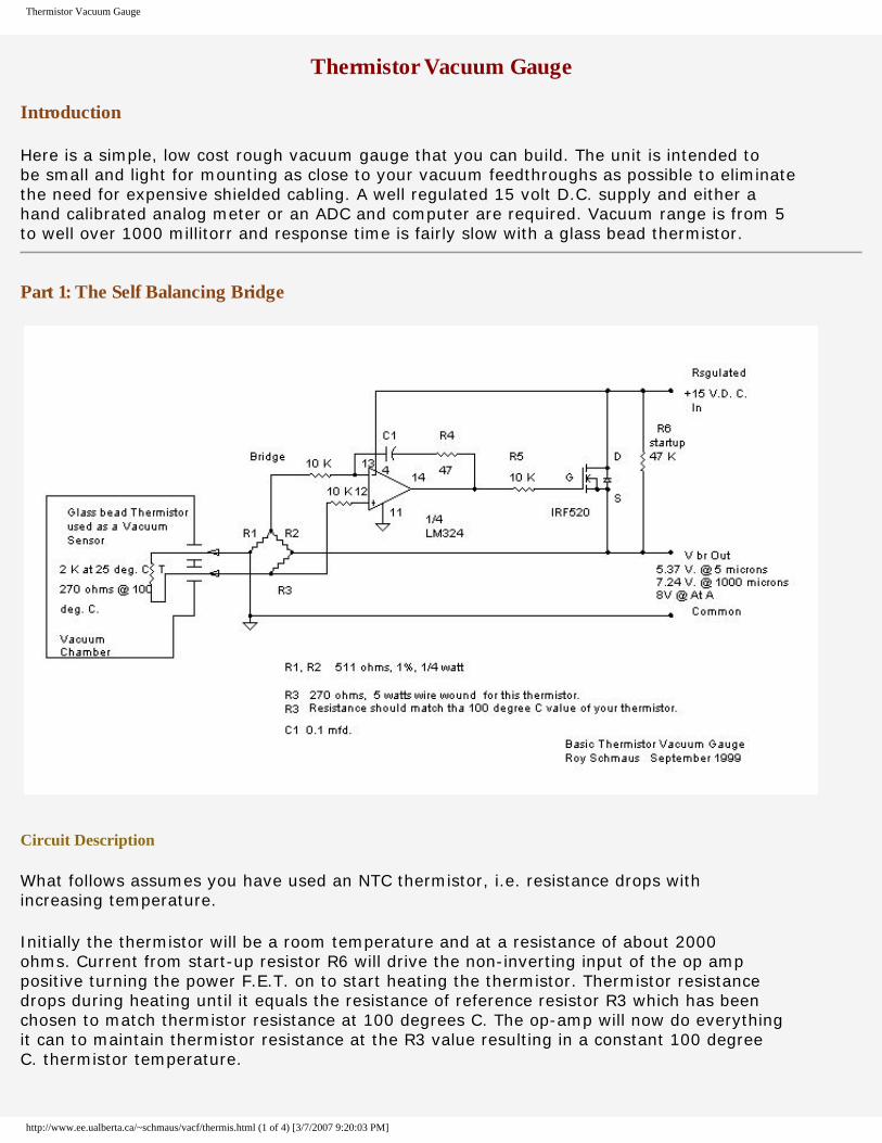
Here is a simple, low cost rough vacuum gauge that you can build. The unit is intended to be small and light for mounting as close to your vacuum feedthroughs as possible to eliminate the need for expensive shielded cabling. A well regulated 15 volt D.C. supply and either a hand calibrated analog meter or an ADC and computer are required. Vacuum range is from 5 to well over 1000 millitorr and response time is fairly slow with a glass bead thermistor.

Part 1: The Self Balancing Bridge

Circuit Description

What follows assumes you have used an NTC thermistor, i.e. resistance drops with increasing temperature.

Initially the thermistor will be a room temperature and at a resistance of about 2000 ohms. Current from start-up resistor R6 will drive the non-inverting input of the op amp positive turning the power F.E.T. on to start heating the thermistor. Thermistor resistance drops during heating until it equals the resistance of reference resistor R3 which has been chosen to match thermistor resistance at 100 degrees C. The op-amp will now do everything it can to maintain thermistor resistance at the R3 value resulting in a constant 100 degree C. thermistor temperature.

http://www.ee.ualberta.ca/~schmaus/vacf/thermis.html (1 of 4) [3/7/2007 9:20:03 PM]


Bridge output voltage is at maximum at Atmospheric pressure and decreases in vacuum due to diminishing heat losses to gas molecules around the thermistor. Minimum voltage is usually around 5 volts at .005 torr vacuum.

Part 2 . The Level Shifter

The subtractor circuit shown above shifts the 5 to 8 volt output from the bridge down to a ground referenced 0 to 2.5 volts. Normally R7 to R10 would all be the same value with R9 connected to a reference voltage equal to whatever the minimum voltage from the bridge was. R9 is connected to the regulated +15 volt supply to reduce component count and consequently is a higher value. R9 will most likely have to be hand trimmed for different thermistors. Don't use programming resistors of less than 100k for the single power supply circuit shown or you will have problems getting the output to go near ground.

Part 3. Results

The graph below is a "quick and dirty" attempt at calibration against a thermocouple gauge on the only vacuum system that was available for testing.



The previous gauge was calibrated against a Granville Philips 'Convectron' (TM) Pirani gauge. Results are here

Part 4. Construction Hints

Find a suitable thermistor that is vacuum compatible and with a resistance of about 2000 ohms at 25 degrees C and decreasing resistance with increasing tenperature. Some manufacturer's and supplier's web page links with curves, etc. are included below.

Vacuum feed throughs for the thermistor leads can be quite expensive and hard to find so that one is left up to the user's ingenuity with low vapor pressure epoxy or hermetically sealed surplus connectors.

The electronics is easily assembed on an electronic 'bread board' for initial testing. Be sure to heat sink the power F.E.T. and allow for ventilation of the F.E.T. and R3. Themistor manufacturers warn of drift above 105 degrees C so consult a TC curve and take care in the selection of reference resistor R3.

Once you have the basic gauge working it will require calibration against a reference gauge of some sort. Alternatively if your bridge output is between five and eight volts at Atmospheric pressure other readings may be calculated using the graphs above as a reference. Low cost thermistors vary between individual units so your readings will not be the same as the graph readings but will be shifted up or down.

The bridge circuit shown in Part 1 can also be used with a single filament Pirani gauge if connections to the inverting and non inverting op amp inputs are switched and R3 is reduced to 115 ohms ohms for the old CVC "Autovac" gauge tubes. Outdoor Christmas light filaments seem to have about the right resistance and might also be worth trying for those inclined to experiment.

Conclusion

Originally the control circuit was a Pirani gauge controller we developed to replace some ancient Consolidated Vacuum Corporation ‘Autovac’ gauge control units. With the demise of CVC and with two of their Pirani heads still on a difficult to modify glass teaching system


http://www.ee.ualberta.ca/~schmaus/vacf/oldga.jpg


a replacement for the original vacuum tube unit was necessary. The Pirani controller has proven to be very reliable and accurate and has been in service for ten years with no problems.

A low cost replacement roughing gauge was in demand so we decided to try some glass bead thermistors as vacuum sensing elements and developed the very low-cost, simple circuit shown above. Accuracy and response time are not as impressive as that of the Pirani gauge but still adequate for non-critical applications.

Roy Schmaus September 1999

Thermistor Manufacturer's Links

● Alpha Sensors Excellent technical information including thermistor curves.● General Information About Thermistors from Wuntronics Gmbh.● Thermometrics

Sources

Most local electronics jobbers should be able to supply thermistors from a variety of suppliers. Here are a few suppliers that list low cost glass and epoxy thermistors in their catalogs.

● Digi-Key Thermometrics, Keystone Thermometrics, Panasonic thermistors.

● Electro-Sonic Stock # 135-202FAG-J01 Fenwal Glass encapsulated chip thermistor, 2k at 25 degrees C. $5.92 Cdn.

● Newark Philips, Thermometrics thermistors

References

● The Burr Brown Handbook of Operational amplifier Applications● The National Semiconductor Corporation Linear Data Book● The International Rectifier HEXFET Power MOSFET Data Book

© 1999,2000 by Roy Schmaus

Back


http://www.alphasensors.com/

http://www.wuntronic.de/sensors/thermistor.htm

http://www.thermometrics.com/htmldocs/numindex.htm

http://www.digikey.com/

http://www.e-sonic.com/

http://www.newark.com/

http://www.ee.ualberta.ca/~schmaus/vacf/hamsci.html

The output and sensitivity of vacuum gauges using a heated element in a Wheatstone bridge


1969 J. Phys. E: Sci. Instrum. 2 305


Download details:

IP Address: 143.106.72.69















Journal of Scientific Instruments (Journal of Physics E) 1969 Series 2 Volume 2

The output and sensitivity of vacuum gauges using a heated element in a Wheatstone bridge

E M McKay Building Research Station, Garston, Herts.

sensitivity’. The application of the load-line technique is also discussed, in some detail. It is shown that a useful insight may be gained, by this method, into the interdependence of the element and its associated bridge, MS received 9 October 1968, in reaised form 13 January 1969

Abstract This paper deals with design methods for Pirani and related gauges. The analytical approach is discussed, with particular reference to bridge classification and ‘gauge

that it may be used over the whole range for which the output is pressure dependent and with equal facility for both metallic filament and thermistor elements.

1 Introduction The vacuum gauge employing a heated element in a Wheat- stone bridge network has received considerable attention since the idea was first proposed by Pirani in 1906. This has given rise to a wide variety of both elements and circuitry, in terms of the pressure range covered, sensitivity, independ- ence of ambient temperature fluctuation, response time, etc.

Such instruments are not capable of absolute calibration, due to the existence of empirical parameters in any expression relating pressure to the measured quantity. Furthermore these expressions become unwieldly if they include terms relating to all the modes of heat transfer from the element; this would be especially so for the thermistor element with its nonlinear resistance-temperature relation. By making certain assump- tions, generally based on the relative importance of the various components in the heat transfer equation (and by implication on the pressure range), various approximate relations have however been derived. Examples of these will be discussed later.

This paper will be concerned with the ways in which design problems may be dealt with in so far as they relate to gauge output and sensitivity. 2 Types of gauge circuit Pirani’s proposal for the basic classification of thermal conductivity gauge circuits is set out elsewhere (see Pirani and Yarwood 1961). As pointed out by Dunoyer (1949) some of the circuits used by Pirani did not correspond exactly to this classification. It might also be noted that there is still some confusion regarding the terminology applied to these circuits. For example, a gauge employing a constant voltage bridge is often referred to as one of the ‘constant voltage’ type although it is also quite possible (and indeed sometimes desirable) to maintain the element current constant, by means of suitably chosen bridge arms and detector. According to the Pirani classification this gauge might then be referred to as one of the ‘constant current’ type.

Because of this confusion about terminology, and considering the ways in which bridge circuits may be conveniently analysed, it might be more useful if the following classification were adopted. In the first instance bridges may be classified as either (a) balanced or (b) unbalanced. Further subdivision could then be made according to the detector used. Thus those referred to previously as ‘constant voltage’ or ‘constant

3”

current’ may be considered simply as particular cases of the general unbalanced bridge circuit. 3 The unbalanced bridge method As mentioned in the introduction, this paper will be concerned only with the gauge sensitivity and output as a function of pressure. In terms of the definitions to be given these are directly related and only one really needs to be considered. In this section the analytical approach will be discussed.

Firstly it is important to emphasize that no single relationship exists between the element power dissipation P and the pressure p , which is valid for all pressures. It follows therefore that there cannot be a single relationship between gauge output and pressure except possibly over a restricted range. Even then the relative importance of individual parameters might well be difficult to assess. The papers of Kersten and Brinkman (1949) and Veis (1959) are especially valuable for an understanding of the difficulties associated with complete gauge analysis. That by Corruccini (1957) gives a good account of the conduction of heat from an element in an evacuated enclosure. 3.1 Sensititlity In the literature, various meanings are attributed to the term sensitivity. Thus, for the present purpose gauge sensitivity Sg is defined as

S g = diW/dp (1)

U here iM is the measured signal. In order to see the relative effects of the gauge element and the Wheatstone bridge, equation (1) may usefully be rewritten as

(2) RdM1 dR & - - - dR Rdp

= s b Se, say

where s b is the bridge sensitivity, given by

and Se is the element sensitivity, given by

1 dR S e = - -.

R dP

(3)

(4)

( 5 )

305

E A4 McKay

This may be written more conveniently as

(6) 1 dR dTe Se=---, RdTe dp

Thus for a metallic filament subjected to a sufficiently small change in temperature we may write

where 31 is the temperature coefficient of resistance. For a thermistor type element, having a resistance-temperature relation given approximately by

R = R exp(B/Te)

we have for its sensitivity the expression

Whilst it has been proposed that the gauge sensitivity may be considered as the product of bridge and element sensitivi- ties, it should be stressed that the latter, if considered in detail, will also be found to depend on the bridge circuit used. An example of the analysis has been given elsewhere (McKay 1967 M.Sc. Thesis, University of London) in which the high impedance detector was assumed and the gauge element was taken to be of the metallic filament type. Then, consideration was given to heat trans€er by conduction, radiation and to some extent that through the terminals, but not to heat transfer by convection. 3.2 Bridge sensitiuity The term bridge sensitivity as used in this paper has been defined in equation (4), where a single variable element R is assumed. If the reference condition is that of balance, and s b is constant, it will be seen that this agrees with another defi- nition often given, i.e. s b = RM/6R, since 6M= (144 - 0) = M.

The analysis of gauge circuits in order to derive expressions for bridge sensitivity is most conveniently carried out using ThCvenin's theorem. This in terms of the notation given in figure 1 enables us to write for our equivalent generator

where f is the fractional change in R, i.e. 6RiR and its internal resistance RT given approximately by

S+ R 1 + n

RT=-

where n= R/P=S/Q at balance.

for us to write Generally speaking, the magnitude off is sufficiently small

the degree of approximation depending obviously on the bridge ratio n, as will be shown.

From the equivalent circuit of figure l(6) and using equations (9) and (10) we then have for the high impedance detector

and for the low but finite impedance detector

(13) n f 1

Io = ~ (1+n)2 { (S+R)+( l+n)D}

If sufficiently small values o f f are assumed, as referred to above, both equations (12) and (13) will be seen to give a

(0) ( b )

Figure 1 detector

Transformation of Wheatstone bridge, as seen by

linear relation between the output and the fractional resistance change.

To assess the usefulness of the approximate relations for VO and IO for small values of A the errors E involved for a number of typical cases have been evaluated. Thus for an equi-arm bridge, each arm of resistance 100 R, and the ratio of f.s.d. voltage of the detector (high impedance) to f.s.d. voltage of the supply of 0.01 the following values were obtained: n = l , 6 6 2 % ; n=10, ~ 6 8 . 5 % ; n=0,1, ~ 6 1 . 1 % . For the current output bridge, by using a detector of 100 R and a ratio of f.s.d. current to supply voltage of 20 PA v-l it may also be shown that: for n= 1, ~ < 0 4 3 % ; for n = 10, ~ ~ 2 3 % ; for n=0.1, ~ 6 2 % .

The effect of the bridge ratio is clearly seen to be more marked for n = 10 in both cases. Also it will be appreciated that errors will be less than those given when deflection is less than full scale. 4 The balanced bridge The second basic class of gauge proposed in this paper operates with negative feedback applied to retain the element at constant resistance (and temperature). Significant advant- ages accrue with this method, as will be seen from the folloming sections. 4.1 Fundamental equations The expression for rate of heat transfer from the element in the balanced condition is given by :

=f(p, Te, Tal+&, Te, Ta)+h(Te, Ta)+j(Te, Ta) (14)

\$here C is a constant determined by the bridge arms at balance, i.e. C= R:(P+ R), T, is the element temperature and T, is the envelope temperature; the terms f(p, Te, Ta), g(p, Te, Ta) and h(Te, Ta) are respectively due to conduction through the gas, convection through the gas and radiation, and j(Te, Ta) is due to conduction through the terminals (assumed independent of pressure).

Thus from equation (14) we see that

\\here V B ~ and V B ~ are the bridge voltages needed for a balanced condition at pl and p~ respectively, the element temperature Te being the same in each case.

An account of terminal losses may be found in von Ubisch (1947) and Leck (1964). The effect of the element (an enclosed heat source) on the envelope temperature has been assessed by English et al. (1965).

306

Thermal vacuum gauges: a study of design techniques

4.2 Sensitivity Due to the existence of the squared voltage term on the left- hand side of equation (15) it might be more convenient to express gauge sensitivity SE, for this mode of operation, as

If adopted, this leads to

allowing in this case the function j to be pressure dependent. It \till be seen, however, that the effect of this term is only by virtue of the relative magnitudes of the derivatives and not of the absolute magnitudes. 5 Application of the load-line technique To avoid the difficulties of an analytical approach based on inadequate equations an alternative approach using the load-line technique may be used. Thus with the aid of a family of element voltagecurrent characteristics (with p and T, as parameters) the superimposition of the load-line enables the calibration curve to be readily obtained. This method offers the significant advantage that it may be applied over the mhole range for which the operating point (V,, le) varies with pressure. Thus it is not necessary to know the absolute or relative magnitudes of the various components of heat transfer. Furthermore it may be applied with equal facility to all gauge circuits, and for both metallic filament and thermistor elements. 5.1 Voltage-current characteristic for gauge element The circuits shown in figure 2 represent the way in which the basic bridge circuit may be transformed into a simple series circuit comprising the gauge element R and an equivalent

I x - ( 0 )

Figure 2 Transformation of bridge circuit, as seen by element

generator for the bridge, its supply and detector, D. The development from (a) to (b) is by means of the T , T network transformation and that from (b) to (c) is achieved by using Thevenin's theorem.

Thus, using the notation of figure 2, we have for the T to T transformation,

__ _ _ ~

A = - PQ T '

PD B=- T '

where T= P+ Q + D ; for the application of Thevenin's theorem, for (b) to (c) we have

(19) A(C+S) vT'=C+S V B , RT'=B+-

C + S + A C+S+A'

For the redrawn bridge circuit we then have for the element R the current and voltage given by

On substitution from above and re-arranging we may write

This will be seen to satisfy the two limiting conditions for the detector impedance D, thus (i) as

D+ cc -voltage output bridge

Ve+ ~ V B R + P

(ii) as D+ 0 - current output bridge

(22)

Now with the aid of the circuit reduced to that shown in figure 2(c) and the expressions obtained for VT' and RT' we may obtain the load line or circuit characteristic. This is given by the equations

or

These show the load line to be a straight line. In figure 3 typical families of voltage-current characteristics

with load-lines superimposed are given (a) for a metallic filament element and (b) for a thermistor. The sign of a is seen to produce a marked difference between them since for the thermistor there is the possibility of a load-line giving more than one operating point at a given pressure. This is illustrated by C'C" in figure 3(b). Thus VT' and RT' require special consideration with this type of element.

The technique will now be illustrated by showing its application to various circuits. These will be idealized for the sake of convenience by assuming a bridge source of negligible impedance and a detector of either high or low impedance. 5.2 Unbalanced bridge with high impedance detector Assuming D+ a, i.e. l0+0, then the output voltage VO is given by

Vo=(Ve- Vs) (25)

i.e. VO = (V, - constant).

This means the gauge sensitivity Sg is given by

It should be noted that for this case the effective generator resistance, i.e. the one which determines the slope of the load line, reduces simply to that of the arm adjacent to the element, i.e. R.c'=P. Also for this condition VT'= VB.

The output voltage is obtained from figure 4 by the hori- zontal displacement of the operating point. Thus if the bridge is initially balanced for p=O, then V0=6Ve since VB is constant. If now we assume a different bridge supply voltage but the resistances remain fixed, then the new load line is simply parallel to the first with its intercept on the Ve axis at the ne% bridge supply. Here for the same pressure change as before the new output voltage is seen to be VO'= 6 Ve'.

It will be seen from the characteristics of both the positive and negative temperature coefficient elements that there will

1

N P + Q + D ) i D ( Q + S > + S ( P + Q)i {R(P+ Q)+ D(P+R)} { D ( Q + S ) + S ( P + Q)+PQ}+PQ{D(Q+S)+S(P+ Q ) }

Ve=

E M McKay

I

( 0 ) v, ( 6 )

Figure 3 Typical element characteristics (le = k(pTa) f( V,)) of (a) metallic filament and (b) thermistor types, wjith load lines superimposed

generally be a difference in output voltage, for a given pressure change, depending on the choice of VB.

The second factor, i.e. that of scale linearity, is possibly more important than the actual magnitude of the voltage change SVe. This is because the amplification of the signals involved is a comparatively straightforward exercise even for the d.c. signals normally employed. However, the effect of nonlinearity may be put to good use by making the gauge more suitable for a given range of pressures. This amounts to scale magnification over a restricted pressure range.

Load-line slope also plays a considerable part in determining gauge operation. This is illustrated in figure 5. It has already been noted that for the bridge under discussion RT’ reduces to P. The lines AC’ and AC” represent the limiting conditions for the load line. The first is that for a constant element voltage whereas the second corresponds to constant element current. Thus line AC’ corresponds to the degenerate bridge form, i.e. as P-+ 0 and the fully supply voltage is permanently across the element. The second line AC” also represents a

degenerate bridge form if the constant current is achieved by means of P+ m, since then we have simply one bridge arm open circuit. This condition could alternatively be achieved by way of a constant current bridge supply, but would of course require a different equivalent generator to the one previously derived for the constant voltage source.

It is then readily seen from figure 5 that the slope of the load-line provides another method whereby the gauge output, sensitivity and scale shape may be controlled. For the hot wire element we may deduce an increasing voltage output as the constant current condition is approached. There is, however, considerable loss of linearity, the relative separation at higher pressures being considerably reduced. When a thermistor is used, figure 5(b) indicates clearly that the maximum output voltage does not occur for the constant current condition but when some finite value of P is chosen.

One further possibility exists whereby the output signal may be varied for a given change in pressure. This is by the inclusion of a resistance r in series with the element. If

( Q ) v,

Figure 4 Unbalanced bridge operation with high impedance detector, showing effect of bridge supply voltage VB on output voltage VO (= S Ve)

308

Thermal vacuum gauges: a study of design techniques

( U ) 1.;

Figure 5 Unbalanced bridge operation with high

5 1

impedance detector, showing effect of change in load line slope

outside the element, r may be assumed constant; this amounts simply to an increase in the effective generator resistance by the series addition. Alternatively the series resistor could be included within the gauge envelope. This would amount to the series combination of two gauge elements and if they had temperature coefficients of opposite sign, the resulting characteristic could take any shape between the two extremes shown in figure 3(a) and (6). 5.3 Unbalanced bridge with low impedance detector In the case where the detector impedance D may be assumed to be negligible, it follows that the element voltage and that across the standard resistance S will be equal, i.e. Ve= Vs from figure 2(a).

Now the output current ZO is given by

By using the load-line technique we may obtain the operating point giving the corresponding values of Ve and l e . Then for a given value of P we may compute IO for a given pressure, by using equation (28). This may be taken a stage further by reducing the expression ZO to one involving a single variable only. This may be either the element voltage or current. As an example let us consider the element voltage Ve.

From the general expressions for the Thevenin equivalent generator, equations (19), substitution of D=O gives

(29) S ( P + Q> SPQ S ( P + Q)+PQ ”’ RT’=S(P+ Q)+PQ‘

VT’ =

The element current le, given by

VT‘ - V e l e = ~

R T’

becomes on substitution from equation (29)

( 0 ) Y

Figure 6 Balanced bridge operation

309

E M McKay

which on substitution into equation (28) gives

= constant N constant x Ve.

5.4 The balanced bridge Referring to figures 6(a) and (b), the line OC representing constant resistance has been superimposed on typical hot wire and thermistor characteristics. This line is taken to be the operating resistance for the element and the intercepts give as before the operating points for given pressures. Through these would be drawn lines of constant slope corresponding to the equivalent source resistance (as seen by the gauge element), The intercepts on the voltage axis would then give the bridge voltage needed to obtain the balanced condition. Calibration may then be achieved by simply plotting the pressures p a , PB, etc. against the corresponding supply voltages VA, VB, etc. It should be remembered that whilst for a balanced bridge the choice of R fixes the value of P S / Q it does not fix the slope of the load-line. Thus any range of supply voltage is permitted. It will be seen, however, that fixing R will give a fixed ratio VB/VA for given pressures PA and PB.

A clear distinction in the use of the two types of element in the balanced bridge mode is seen from figure 6. This is that only in the case of the thermistor will the constant resistance line readily cut the element characteristic for atmospheric pressure. A final point regarding thermistors used in this way is that there is no possible ambiguity of operating point as might occur in the unbalanced bridge. 6 Conclusions The inadequacy of the expressions developed for the sensitivity of gauges employing a heated element in a Wheatstone bridge circuit, e.g. the Pirani and thermistor gauges, results from two factors. Firstly there is the difficulty of developing a useful formula to cover more than a very restricted range. Secondly there is the problem of empirically determined parameters which vary bith time and use. An alternative to the analytical approach, in gauge design, has been discussed, i.e. a graphical approach based on the load-line technique. This has the distinct advantage of not requiring knowledge of the mechanism of heat transfer from the element, thus permitting use over the whole range for ahich the element is sensitive to pressure variation. References Corruccini R J 1957 Vacuum 7 19-27

Dunoyer L 1949 Le Vide 4 571-84

English J Fletcher B and Stechelmacher W 1965 J. Sci. Instrum. 42 77-80

Kersten J A H and Brinkman H 1949 Appl. Sci. Res. 41 289-305

Leck J H 1964 Pressure Measurements in Vacuum Systems 2nd edn (London: Chapman and Hall)

Pirani M 1906 Deutsche Phys. Ges. Verk. 8 686

Pirani M and Yarwood J 1961 Principles of Vacuum Engineering (London : Chapman and Hall)

von Ubisch H 1947 Arkit?. F. Mat. Astra. Och. Fy,s. 34A NO. 14 1-33

Veis S 1959 Vacuum 9 186-9

310

Documents

F 609 Relatorio Final Pirani - ifi.unicamp.brlunazzi/F530_F590_F690_F809_F895/F809/... · O Pirani é um instrumento utilizado para medir pressão na faixa de 200 a 10-4 torr (baixo