Hugo Miguel Ferreira Beleza

Estimation of the glottal flow from the speech or

singing voice

Dissertação de Mestrado

Mestrado em Bioinformática

Trabalho efetuado sob a orientação dos

Professor Doutor Rui Manuel Ribeiro Castro Mendes

Professor Doutor Aníbal João de Sousa Ferreira

Janeiro de 2016

ii

DECLARAÇÃO

Nome: Hugo Miguel Ferreira Beleza

Título da dissertação: Estimation of the glottal flow from the speech or singing voice

Orientadores:

Professor Doutor Rui Manuel Ribeiro Castro Mendes

Professor Doutor Aníbal João de Sousa Ferreira

Ano de conclusão: 2016

Mestrado em Bioinformática

É AUTORIZADA A REPRODUÇÃO INTEGRAL DESTA DISSERTAÇÃO APENAS PARA EFEITOS DE

INVESTIGAÇÃO, MEDIANTE DECLARAÇÃO ESCRITA DO INTERESSADO, QUE A TAL SE

COMPROMETE.

Universidade do Minho, 15/01/2016

Assinatura:

iii

RESUMO

O processo de produção humana de voz é, resumidamente, o resultado da convolução entre o sinal de

excitação, o impulso glótico, e a resposta impulsiva resultante da função de transferência do trato

vocal. Este modelo de produção de voz é frequentemente referido na literatura como um modelo fonte-

filtro, em que a fonte representa o fluxo de ar que sai dos pulmões e passa pela glote (espaço entre as

pregas vocais), e o filtro retrata as ressonâncias do trato vocal e a radiação labial/nasal.

Estimar a forma do impulso glótico a partir do sinal de voz é de importância significativa em diversas

áreas e aplicações, uma vez que as características de voz relacionadas, por exemplo, com a qualidade

da voz, esforço vocal e distúrbios da voz, devem-se, principalmente, ao fluxo glotal. No entanto, este

fluxo é um sinal difícil de determinar de forma direta e não invasiva.

Ao longo das últimas décadas foram desenvolvidos vários métodos para estimar o impulso glótico mas

sem o desenvolvimento de um algoritmo eficiente e automático. A maioria dos métodos desenvolvidos

baseia-se num processo designado por filtragem inversa. A filtragem inversa representa a

desconvolução, ou seja, procura obter o sinal de entrada aplicando o inverso da função de

transferência do trato vocal ao sinal de saída. Apesar da simplicidade do conceito, o processo de

filtragem inversa não é simples uma vez que o sinal de saída pode incluir ruído e não é alcançável

modelar com precisão as características do filtro do trato vocal.

Nesta dissertação apresentamos um novo método de filtragem de um sinal de modo a melhorar um

método robusto de estimação da fonte glótica, no domínio das frequências, que usa uma característica

de fase baseada nos Atrasos Relativos Normalizados (NRD) dos harmónicos. Este modelo é aplicado a

diversos sinais de voz (sintéticos e reais), e os resultados obtidos da estimação do impulso glótico são

comparados com os obtidos usando outros métodos analisados no estado da arte com e sem o

referido método de filtragem.

Palavras-Chave: impulso glótico, estimação do impulso glótico, filtragem inversa, integração no domínio

das frequências, estimação do impulso glótico no domínio das frequências.

v

ABSTRACT

The human speech production system is, briefly, the result of the convolution between the excitation

signal, the glottal pulse, and the impulse response resulting from the transfer function of the vocal tract.

This model of voice production is often mentioned in the literature as a source-filter model, where the

source represents the flow of the air leaving the lungs and passing through the glottis (space between

the vocal folds), and the filter stands for the resonances of the vocal tract and the lip/nostrils radiation.

The estimation of the shape of the glottal pulse from the speech signal is of significant importance in

many fields and applications, since the most important features of speech related to voice quality, vocal

effort and speech disorders, for example, are mainly due to the voice source. Unfortunately, the glottal

flow waveform which is at the origin of the glottal pulse, is a very difficult signal to measure directly and

non-invasively.

Several methods to achieve the estimation of the glottal flow have been proposed over the last decades,

but an efficient and automatic algorithm which performs reliably is not yet available. Most of the

developed methods are based on the inverse filtering method. The inverse filtering approach represents

a deconvolution process, i.e., it seeks to obtain the source signal by applying the inverse of the vocal

tract transfer function to the output speech signal. Despite the simplicity of the concept, the inverse

filtering procedure is complex because the output signal may include noise and it is not straightforward

to accurately model the characteristics of the vocal tract filter.

In this dissertation we discuss a new filtering method for voiced signals with the goal to improve the

assessment of a robust frequency-domain algorithm for glottal source estimation that uses a phase-

related feature based on the Normalized Relative Delays (NRDs) of the harmonics. This model is applied

to several speech signals (synthetic and real), and the results of the estimation of the glottal pulse are

compared with the ones obtained using other state-of-the-art methods with and without the presence of

that filtering method.

KEYWORDS: glottal pulse, estimation of the glottal pulse, filter, algorithm, frequency-domain glottal source

estimation.

vii

CONTENTS

Resumo.............................................................................................................................................. iii

Abstract............................................................................................................................................... v

List of Figures ................................................................................................................................... viii

List of Table ....................................................................................................................................... ix

Acronyms ........................................................................................................................................... X

1. Introduction ................................................................................................................................ 1

1.1 Motivation ........................................................................................................................... 4

1.2 Goals .................................................................................................................................. 4

2. Vocal Organs .............................................................................................................................. 5

2.1 Anatomy & Physiology ......................................................................................................... 5

2.2 Glottal Flow ......................................................................................................................... 9

3. Glottal Flow Estimation Algorithms ............................................................................................. 13

3.1 Representative Estimation Algorithms ................................................................................ 13

3.1.1 Iterative Adaptive Inverse Filtering Algorithm ............................................................... 15

3.1.2 Complex Cepstrum Decomposition ............................................................................ 17

3.1.3 Frequency-Domain Glottal Pulse Estimation ................................................................ 19

3.2 Glottal Flow Parameterization ............................................................................................ 22

3.3 Applicability in Biomedical Applications .............................................................................. 25

4. Experimental Tests .................................................................................................................... 29

4.1 Tests with Synthetic Speech Signals .................................................................................. 30

4.1.1 Parks-McClellan Algorithm ......................................................................................... 31

4.2 Tests with Real Speech Signals .......................................................................................... 31

5. Results & Discussion ................................................................................................................. 33

5.1 Synthetic Speech Signals ................................................................................................... 33

5.2 Real Speech Signals .......................................................................................................... 42

6. Conclusion ................................................................................................................................ 47

Bibliography ..................................................................................................................................... 49

viii

LIST OF FIGURES

Figure 1 - Cycles from a voiced speech signal showing the voice source signal..................................... 3

Figure 2 - Illustration of the LPC method. ............................................................................................ 4

Figure 3 – The respiratory system. ...................................................................................................... 5

Figure 4 - Anterior and posterior views of the larynx and the cartilages ................................................. 6

Figure 5 - Vocal folds as seen from above ........................................................................................... 7

Figure 6 – Speech production model................................................................................................. 10

Figure 7 – Glottal flow waveform ....................................................................................................... 10

Figure 8 - ZZT decomposition algorithm ............................................................................................. 15

Figure 9 - Block diagram of the Iterative Adaptive Inverse Filtering method ......................................... 16

Figure 10 - Block diagram of the Complex Cepstrum-based decomposition. ....................................... 18

Figure 11 – Block diagram of FD-GPE algorithm ................................................................................ 20

Figure 12 - The flow pulse phases ..................................................................................................... 22

Figure 13 – Group delay of the synthesized female signals ................................................................ 34

Figure 14 – Group delay of the synthesized male signals ................................................................... 35

Figure 15 – Frequency magnitude response of the female synthesized speech. ................................. 36

Figure 16 – Frequency magnitude response of the male synthesized speech. .................................... 37

Figure 17 - Glottal flow derivative estimation of female vowel “a”. ...................................................... 38

Figure 18 - Glottal flow estimation of female vowel “a” ...................................................................... 38

Figure 19 - Glottal flow derivative estimation of female vowel “i”. ....................................................... 39

Figure 20 - Glottal flow estimation of female vowel “i” ....................................................................... 39

Figure 21 - Glottal flow derivative estimation of male vowel “a”. ......................................................... 40

Figure 22 - Glottal flow estimation of male vowel “a” ......................................................................... 40

Figure 23 - Glottal flow derivative estimation of male vowel “i”. .......................................................... 41

Figure 24 - Glottal flow estimation of male vowel “i” .......................................................................... 41

Figure 25 - Glottal flow estimation of the female subject vowel “a” ..................................................... 43

Figure 26 - Glottal flow estimation of the woman’s vowel “i” .............................................................. 43

Figure 27 - Glottal flow estimation of male subject vowel “a” ............................................................. 44

Figure 28 - Glottal flow estimation of the man’s vowel “i” .................................................................. 44

ix

LIST OF TABLE

Table 1 – SNR results for the synthetic signals .................................................................................. 42

Table 2 – SNR results for the human speech. ................................................................................... 45

ACRONYMS

ANN – Artificial Neural Network

CP – Closed Phase

ClQ – Closing Quotient

DAP – Discrete All-pole Modelling

DFT – Discrete Fourier Transform

EGG – Electroglottographs

F0 – Instantaneous Fundamental Frequency

FD-GPE – Frequency-Domain Glottal Pulse Estimation

FIR – Finite Impulse Response

GCI – Glottal Closure Instant

GHNR’ – Glottal Related Harmonic-to-Noise Ratio

GIF – Glottal Inverse Filtering

GMM – Gaussian Mixture Model

GOI – Glottal Opening Instant

HNR – Harmonic-to-Noise Ratio

HRF – Harmonic Richness Factor

IAIF – Iterative Adaptive Inverse Filtering

IIR – Infinite Impulse Response

LF – Liljencrants-Fant

LP – Linear Prediction

LPC – Linear Predictive Coding

MFC – Mel Frequency Cepstral

NAQ – Normalized Amplitude Quotient

NRD – Normalized Relative Delay

OP – Open Phase

OQ – Open Quotient

PCA – Principal Component Analysis

PD – Parkinson Disease

SJE – Spectral Jitter Estimator

SNR – Signal to Noise Ratio

SQ – Speed Quotient

SVLN – Separation of the Vocal tract with the Liljencrants-Fant model plus Noise

SVM – Support Vector Machine

UC – Unit Circle

ZZT – Zeros of Z-Transform

1

1. INTRODUCTION

Mankind is well-known for countless characteristics and one of those is socialization. The basic

mechanism used to fulfill their social needs is through communication and therefore humans use their

vocal organs to execute a process, entitled phonation, generating the man’s most natural

communication technique, speech. Although people do not realize, since speech is very present in our

everyday life, voicing is a very complex phenomenon that delivers a high rate of information and

constitutes a combinatory system in which syllables can be mixed into a large number of sequences

originating words that are combined to form phrases. Due to this complexity, speech is a research goal

in several areas such as engineering, medicine, phonetics, linguistics, phoniatrics and singing. Another

example of voicing complexity is that even after quite a few decades of research not all of its features

are known and documented. All the fields of speech science are based on the utilization of the speech

pressure waveform which can be difficult based on the fact that humans are capable of varying

extensively the functioning of their vocal organs due to the utterance produced, the language, the

gender and the emotional state of the speaker among others. Flanagan, in 1972, categorized speech

sounds into three main classes according to the mechanism of production: voiced sounds, which result

from a quasi-periodic vibration of the vocal folds; unvoiced sounds, where the sound excitation is

turbulent noise and plosives, which are transient-type sounds made up by abruptly releasing the air flow

that has been blocked by the lips[1]. Vowels, a sub-category of voiced sounds, represent the research

goal of most interest because of their crucial phonetic role in most languages.

The phonation process has three main groups of organs involved. The first group are the lungs which

are the source of energy to provide an airflow that passes though the trachea and reaches the second

main group, the larynx, where the modulation of the airflow occurs. Present in the larynx are the vocal

folds, a very important component of phonation, and the glottis, the space comprised between the vocal

folds. The glottal modulation provides either the quasi-periodic vibration or the turbulent noise to the

last main group, the vocal tract. This group is constituted by the pharyngeal, oral and nasal resonant

cavities and here is where the airflow is shaped in terms of timbre. Finally, the airflow reaches and

pressures the lips as a velocity flow that results in speech. This airflow is commonly called the glottal

flow. The glottal behavior manipulates both pitch and volume, as well as the voice quality. Pitch

represents the perceived fundamental frequency of a voiced sound and, along with volume, represents

2

important features for controlling stress and intonation of speech. Voice quality is a measure of the

laryngeal phonation style and provides paralinguistic information. Glottal flow processing refers to the

methods that study the estimation, modeling and characterization of the glottal source, as well as the

integration of associated information. Estimation of the glottal flow is quite challenging, as the oscillation

of the vocal folds can neither be examined directly due to their hidden position in the larynx nor be

observed without aids because of the high speed of the oscillations. The methods developed are

grounded on visual, electrical and electromagnetic methods. Visual analysis is widely used with

numerous techniques, such as video stroboscopy, digital high-speed stroboscopy and kymography.

Other type of devices such as electroglottographs (EGG) or laryngographs measure the impedance

between the vocal folds, which is an indirect image of the glottal opening. High-speed imaging implies

introducing a laryngoscope positioned in such a way as to allow visualization of the larynx.

Unfortunately, acquiring visual information requests for invasive measurements and, although they are

informative about the glottal behavior, these methods only analyze an image of the real glottal flow.

Fortunately, an alternative to the analysis methods referred above exists, by acoustically investigating

the functioning of the human speech production mechanism with several mathematical models.

Most models of the voice production system assume that voice is the result of an excitation signal

which is modulated by a filter function that is determined by the shape of the vocal tract. This is

frequently mentioned as a source-filter approach. In several speech processing applications, separating

source and filter is important as the separation could lead to the distinct characterization and modeling

of the two features. This is advantageous since these two components act on different properties of the

speech signal, but it is also one of the most difficult challenges in speech processing, since neither the

glottal or the vocal contributions are observable in the speech waveform. The glottal flow process can

be divided into three main steps[2]:

i. Synchronization with the glottal cycles. In this step the frequency of vibration of the vocal folds,

also known as instantaneous fundamental frequency (F0), the polarity of the speech signal and

the instants of significant excitation in each glottal cycle (called Glottal Closure Instants (GCIs))

are determined (Figure 1);

ii. Estimation and parameterization of the glottal flow. In the second step, the glottal flow is

estimated from the speech signal. The glottal flow estimate is then parameterized by extracting

relevant features;

3

iii. Incorporation of the glottal information in the target application. In this last step, the resulting

glottal information is used to increase the performance of a voice technology application.

Figure 1 - Cycles from a voiced speech signal showing the voice source signal. The glottal closing instant (GCI), glottal opening instant

(GOI), the closed phase (CP) and open phase (OP) are indicated[3].

Due to the aforementioned limitations, using the real glottal flow in standard speech processing

systems is commonly avoided. It is usual to consider, for the filter, the contribution of the spectral

envelope of the speech signal, and for the source, the residual signal obtained by glottal inverse filtering

(GIF). The idea of GIF is to custom a computational model for the filtering effects of the vocal tract and

lip radiation and then to cancel these effects from speech by filtering the recorded signal through the

inverses of the vocal tract and lip radiation model. GIF aims to estimate the input of the vocal system

(the glottal excitation) using just the output, i.e. the speech signal. In most GIF methods, the estimation

of the vocal tract and lip radiation is computed from the acoustical speech pressure signal, which

makes the analysis non-invasive. This technique is typically used in association with parameterization of

the estimated glottal flow in order to describe voice production quantitatively. Methods that

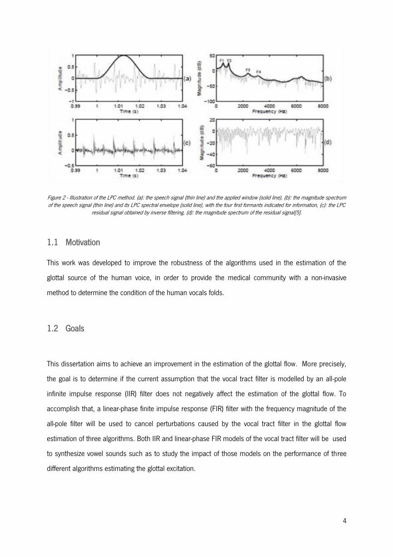
parameterize the filter, such as the Linear Predictive Coding (LPC) (Figure 2) or Mel Frequency Cepstral

(MFC) features, are widely used in practically every field of Speech Processing[4]. Contrarily to the

methods mentioned above, techniques modeling the excitation signal are still not well proven and there

might be knowledge to extract by combining these modeling methods with several applications.

4

Figure 2 - Illustration of the LPC method. (a): the speech signal (thin line) and the applied window (solid line), (b): the magnitude spectrum of the speech signal (thin line) and its LPC spectral envelope (solid line), with the four first formants indicated for information, (c): the LPC

residual signal obtained by inverse filtering, (d): the magnitude spectrum of the residual signal[5].

1.1 Motivation

This work was developed to improve the robustness of the algorithms used in the estimation of the

glottal source of the human voice, in order to provide the medical community with a non-invasive

method to determine the condition of the human vocals folds.

1.2 Goals

This dissertation aims to achieve an improvement in the estimation of the glottal flow. More precisely,

the goal is to determine if the current assumption that the vocal tract filter is modelled by an all-pole

infinite impulse response (IIR) filter does not negatively affect the estimation of the glottal flow. To

accomplish that, a linear-phase finite impulse response (FIR) filter with the frequency magnitude of the

all-pole filter will be used to cancel perturbations caused by the vocal tract filter in the glottal flow

estimation of three algorithms. Both IIR and linear-phase FIR models of the vocal tract filter will be used

to synthesize vowel sounds such as to study the impact of those models on the performance of three

different algorithms estimating the glottal excitation.

5

2. VOCAL ORGANS

2.1 Anatomy & Physiology

The respiratory system consists of the nasal cavity, the pharynx, the larynx, the trachea, the bronchi,

and the lungs (Figure 3). The term upper respiratory tract refers to the nose, the pharynx, and

associated structures; and the lower respiratory tract includes the larynx, trachea, bronchi, and lungs.

Figure 3 – The respiratory system.

The nose, consists of the external nose and the nasal cavity. The external nose is the visible structure

that forms a prominent feature of the face. The nasal cavity extends from the nares to the choanae. The

nares, are the external openings of the nasal cavity and the choanae are the openings into the pharynx.

The hard palate is a bony plate that forms the floor of the nasal cavity that separates the nasal cavity

from the oral cavity. The nasal cavity has several functions:

i. The nasal cavity is a passageway for air that’s open even when the mouth is full of food.

ii. The nasal cavity cleans the air. The vestibule is lined with hairs that trap some of the large

particles of dust in the air. The mucus traps debris in the air, and the cilia on the surface of the

mucous membrane sweep the mucus posteriorly to the pharynx.

iii. The nasal cavity humidifies and warms the air. Moisture from the mucous epithelium and from

excess tears that drain into the nasal cavity through the nasolacrimal duct is added to the air as

it passes through the nasal cavity. Warm blood flowing through the mucous membrane warms

6

the air within the nasal cavity before it passes into the pharynx, thus preventing damage from

cold air to the rest of the respiratory passages.

iv. The olfactory epithelium, the sensory organ for smell, is located in the most superior part of the

nasal cavity.

v. The nasal cavity and paranasal sinuses are resonating chambers for speech.

The pharynx is the common opening of both the digestive and respiratory systems. It receives air from

both the nasal cavity and the oral cavity. The pharynx is connected to the respiratory system at the

larynx. The pharynx is divided into three regions: the nasopharynx, the oropharynx, and the

laryngopharynx.

The nasopharynx is the superior part of the pharynx and extends from the choanae to the soft palate.

The soft palate prevents swallowed materials from entering the nasopharynx and nasal cavity. The

posterior surface of the nasopharynx contains the pharyngeal tonsil which aids in defending the body

against infection.

The oropharynx extends from the uvula to the epiglottis. The oral cavity opens into the oropharynx

through the fauces. Thus, air, food, and drink all pass through the oropharynx.

The laryngopharynx extends from the tip of the epiglottis to the esophagus and passes posterior to the

larynx.

The larynx consists of an outer casing of nine cartilages that are connected to one another by muscles

and ligaments (Figure 4). Six of the nine cartilages are paired, and three are unpaired. The largest of

the cartilages is the unpaired thyroid cartilage, or Adam’s apple.

Figure 4 - Anterior (A) and Posterior (B) views of the larynx and the cartilages. Image from Anatomy & Physiology for Speech, Language and Hearing[6]

7

The most inferior cartilage of the larynx is the unpaired cricoid cartilage, which forms the base of the

larynx on which the other cartilages rest. The third unpaired cartilage is the epiglottis. It’s attached to

the thyroid cartilage and projects as a free flap toward the tongue. During swallowing, the epiglottis

covers the opening of the larynx and prevents materials from entering it.

Two pairs of ligaments extend from the anterior surface of the arytenoid cartilages to the posterior

surface of the thyroid cartilage. The superior ligaments are covered by a mucous membrane called the

vestibular folds, or false vocal cords (Figure 5). When the vestibular folds come together, they prevent

food and liquids from entering the larynx during swallowing and prevent air from leaving the lungs, as

when a person holds breath.

Figure 5 - Vocal folds as seen from above. The true vocal folds appear white upon examination as a result of the superficial layer of squamous epithelial tissue. Seen immediately superior to the true vocal folds are the ventricular folds[6]

The inferior ligaments are covered by a mucous membrane called the vocal folds, or true vocal cords.

The vocal folds and the opening between them are called the glottis. The larynx performs three

important functions:

i. The thyroid and cricoid cartilages maintain an open passageway for air movement.

ii. The epiglottis and vestibular folds prevent swallowed material from moving into the larynx.

iii. The vocal folds are the primary source of sound production. Air moving past the vocal folds

causes them to vibrate and produce sound. The greater the amplitude of the vibration, the

louder is the sound. The force of air moving past the vocal folds determines the amplitude of

vibration and the loudness of the sound. The frequency of vibrations determines pitch, with

higher frequency vibrations producing higher pitched sounds and lower frequency vibrations

8

producing lower pitched sounds. Variations in the length of the vibrating segments of the vocal

folds affect the frequency of the vibrations. Higher pitched tones are produced when only the

anterior parts of the folds vibrate, and progressively lower tones result when longer sections of

the folds vibrate. The sound produced by the vibrating vocal folds is modified by the tongue,

lips, teeth, and other structures to form words. A person whose larynx has been removed can

produce sound by swallowing air and causing the esophagus to vibrate.

Movement of the arytenoid and other cartilages is controlled by skeletal muscles, thereby changing the

position and length of the vocal folds. When only breathing, lateral rotation of the arytenoid cartilages

abducts the vocal folds, which allows greater movement of air. Medial rotation of the arytenoid

cartilages adducts the vocal folds, places them in position for producing sounds, and changes the

tension on them. Anterior/posterior movement of the arytenoid cartilages also changes the length and

tension of the vocal folds.

The trachea is a membranous tube that consists of dense regular connective tissue and smooth muscle

reinforced with 15–20 C-shaped pieces of cartilage. The cartilages protect the trachea and maintain an

open passageway for air. The trachea descends from the larynx to the level of the fifth thoracic vertebra

and divides itself to form two smaller tubes called primary bronchi which extend to the lungs. The most

inferior tracheal cartilage forms a ridge called the carina, which separates the openings into the primary

bronchi. The carina is an important radiologic landmark.

Beginning with the trachea, all the respiratory passageways are called the tracheobronchial tree. Based

on function, the tracheobronchial tree can be subdivided into the conducting zone and the respiratory

zone.

The conducting zone extends from the trachea to small tubes called terminal bronchioles. The

conducting zone functions as a passageway for air movement and contains epithelial tissue that helps

to remove debris from the air and move it out of the tracheobronchial tree.

The primary bronchi divide and continue to branch giving rise to bronchioles. The bronchioles also

subdivide several times to become even smaller terminal bronchioles.

The respiratory zone extends from the terminal bronchioles to small air-filled chambers called alveoli,

which are the sites of gas exchange between the air and blood. The terminal bronchioles divide to form

respiratory bronchioles, which have a limited ability for gas exchange because of a few attached alveoli.

The respiratory bronchioles give rise to alveolar ducts, which are like long branching hallways with many

open doorways. The doorways open into alveoli, which become so numerous that the alveolar duct wall

9

is little more than a succession of alveoli. The alveolar ducts end as two or three alveolar sacs, which

are chambers connected to two or more alveoli.

The right lung has three lobes, and the left lung has two. The lobes are subdivided into

bronchopulmonary segments. The bronchopulmonary segments are subdivided into lobules by

incomplete connective tissue walls. The lobules are supplied by the bronchioles.

2.2 Glottal Flow

The phonetic system, consists of three different systems: the breathing apparatus, the vocal folds and

the vocal tract. The vocal folds are the most important functional components of the voice organ,

because they function as a generator of voiced sounds.

As air rushes through the vocal folds, these may start to vibrate, opening and closing, in alternation, the

passage of air flow, triggering a series of short pulses of air, which increases the supraglottal pressure

and gives rise to the suction phenomenon referred to as the Bernoulli Effect. This effect, due to the

decrease of the pressure across the glottis, sucks the folds back together, and the subglottal pressure

increases again, forcing the vocal folds to open, giving rise to a new pulse of air[7].

The sustained vibration of the vocal folds is described as the balance between three aspects: the lung

pressure, the Bernoulli principle and the elastic restoring force of the vocal fold tissue. The Bernoulli

force, along with the asymmetrical force at the glottis due to the mucosal wave as well as the closed

and open phase of the folds, is considered the sustaining model for vocal fold vibration[8].

The length of the vocal folds is what defines the frequency of vibration of the vocal folds, called the

fundamental frequency. The values of the fundamental frequency of female voices are higher than

those of male voices because frequency is inversely proportional to the length of the vocal folds, as for

female voices, the values of the fundamental frequency are close to 220 Hz while for male voices are

around 110 Hz[9].

The combination of adduction and abduction actions, when performed at certain frequencies, causes

the production of a sound wave that is then propagated towards the lip opening. The sounds produced

as a result of the vibration of the vocal folds are called voiced sounds, and the sounds produced without

vibration of the former are referred to as unvoiced[9].

When the vocal folds vibrate and form pressure pulses near the glottis, the energy of the frequencies of

the excitation is altered as these travel through the vocal tract[10]. Consequently, the sound produced

10

is shaped by the resonant cavities above the glottal source and, therefore, the vocal tract is responsible

for changing acoustically the voice source (Figure 6).

Figure 6 – Speech production model

The shape of the glottal source waveform in a single period is denoted by glottal pulse (Figure 7). As the

vocal folds open and close the glottis at identical intervals, the frequency of the sound generated is

equal to the frequency of vibration of the vocal folds[7].

Figure 7 – Glottal flow waveform

Each cycle consists of four glottal phases: closed, opening, opened and closing. Typically, when the

folds are in a closed position, the flow begins slowly, builds up to a maximum, and then quickly

decreases to zero when the vocal folds abruptly shut[11]. However, studies have indicated that total

closure of the glottis is an idealistic assumption and that the majority of the individuals exhibit some

sort of glottal leakage during the assumed closed phase[12]. Still, most of the glottal models assume

that the source has zero flow during the closed phase of the glottal cycle. The time interval during which

the vocal folds are closed and no flow occurs is referred to as the glottal closed phase. The next phase,

during which there is nonzero flow and up to the maximum of the airflow velocity is called the glottal

opening phase, and the time interval from the maximum to the time of glottal closure is referred to as

the closing or return phase. Many factors can influence the rate at which the vocal folds oscillate

11

through a closed, open and return cycle, such as the vocal folds muscle tension, the vocal fold mass

and the air pressure below the glottis[11].

12

13

3. GLOTTAL FLOW ESTIMATION ALGORITHMS

Glottal-based analysis of speech production consists typically of two stages. In the first stage, glottal flow

waveforms are estimated using signal processing techniques. These techniques generally require

synchronization information such as knowledge of F0 or GCI locations. In the second stage, the

estimated waveforms are parameterized by expressing their most important properties in a compressed

numerical form.

3.1 Representative Estimation Algorithms

During the last 20 years, numerous methods and techniques have been developed for the estimation of

the glottal waveform using voiced speech and it remains an active research field. Miller, in 1951,

published the first study in this field using GIF as the method of estimation[13]. In this, the inverse

model of the vocal tract consisted of lumped analog elements which were adjusted based on visual

observations of the filter output via an oscilloscope in which the tuning of the anti-resonances was done

searching for settings that yielded a maximally flat closed phase of the glottal pulse form. Oppenheim

and Schafer (1968) studied the so-called homomorphic analysis of speech in which the convolved

signal components are transformed into additive components using cepstral analysis[14]. Separation of

speech into the glottal source and vocal tract was studied as an example of Cepstral analysis, hence

presenting the first digital signal processing-based experimental results of GIF. Digital cepstral analysis

has been used to separate the glottal source from the vocal tract. In 1970, Nakatsui and Suzuki

introduced digital filtering as a means to implement the anti-resonances of the vocal tract inverse

model[15]. A GIF technique that is based on inverse filtering the volume velocity waveform recorded in

the oral cavity rather than the acoustic speech pressure signal captured in the free field outside the

mouth was proposed by Martin Rothenberg [16]. A special pneumotachograph mask, as a transducer

capable of measuring the volume velocity at the mouth, recorded the signal which was then subjected

to inverse filtering, where analog antiresonances were determined using spectrographic analysis. The

use of the pneumotachograph mask provides an estimate for the absolute direct DC level of the glottal

airflow, a subject that cannot be achieved with GIF techniques that use the free field microphone

recording as the input. Rothenberg later studied how the pneumotachograph mask could be

optimized[17] and how the mask recordings could be used in the estimation of the glottal area function

14

by utilizing time-varying non-linear inverse filtering[18]. The use of the pneumotachograph mask has

later been combined with digital inverse filtering[19]. Another method, closed phase (CP) covariance

analysis, was proposed by Strube in 1974[20]. The CP analysis method is capable of separating the

glottal source and the vocal tract. The use of linear prediction (LP) introduced a remarkable

improvement in GIF because the vocal tract model adjusts automatically to the underlying speech

signal[21]. The method is sensitive to the extraction of the closed phase region, and even small errors

might result in severe distortion of the estimated glottal excitation[22]. This drawback can be fairly

lessened by using an EGG instead of the acoustic speech signal to estimate the closed phase

region[21]. The performance of CP has been reported to show improvements by using speech samples

from consecutive cycles[22], adaptive high-pass filtering[23] and/or constrained LP in the modulation

of the vocal tract[24]. Computation of a parametric all-pole model of the vocal tract jointly with a source

model, proposed by Milenkovic (1986) as a source of his GIF technique, supports the use of speech

samples over the entire fundamental period in the optimization of the vocal tract, an issue which is not

fulfilled in the basic form of the CP analysis[25]. This method helps with the estimation of the glottal

excitation from high-pitch speech and in sounds where the glottal closure is not completed. A joint

optimization of the vocal tract and glottal source was later used by Fu and Murphy[26]. They have

utilized an approach with the autoregressive model with an exogenous input, where the input has been

represented in a pre-defined parametric form by using the Liljencrants-Fant (LF) model of the voice

source that also involved quantifying the turbulent noise from voiced speech segments.

A innovative idea for the estimation of the glottal excitation, proposed in the studies of Bozkurt, was a

non-parametric method exploiting the maximum-phase properties of the speech signal[27]. Zeros of Z-

Transform (ZZT), does not utilize the LP analysis to estimate the source-tract separation, but rather

expresses the speech sound with the help of the z-transform as a large polynomial (Figure 8). The roots

of the polynomial are separated into two parts, corresponding to the glottal excitation and the vocal

tract, based on their location with respect to the unit circle. Separation based on phase characteristics

fits the phase spectrum of a model to that of the observed signal at harmonic components by

minimizing the mean square phase difference[28]. The technique proposed is different from the true

GIF techniques (e.g. CP, IAIF) in the sense that the glottal source signal is not explicitly computed but

model parameters are rather solved. A method called Separation of the Vocal tract with the Liljencrants-

Fant model plus Noise (SVLN) represents the baseline method the PaReSy is built upon and enables

high-quality voice transformations[29]. The key differences lie in the energy model, the VTF

15

representation and the estimation of the stochastic noise component. SVLN constructs the latter

through a high pass filter of white noise, application of an amplitude modulation parameterized by the

glottal flow vector, and cross fading between consecutive synthesized noise segments. The gain

quantifies the energy level at analysis to control the stochastic energy at the synthesis step[29].

Figure 8 - ZZT decomposition algorithm (UC acronyms unit circle and DFT acronyms discrete Fourier transform)[27].

3.1.1 Iterative Adaptive Inverse Filtering Algorithm

Iterative Adaptive Inverse Filtering (IAIF) (Figure 9), a straightforward and semi-automatic GIF method

proposed by Alku in 1992, estimates the contribution of the glottal excitation on the speech spectrum

with a low order LP model that is computed with a two-stage procedure[30]. The vocal tract is then

estimated using either conventional LP or discrete all-pole modeling (DAP) that utilizes the Itakura-Saito

distortion measure[31].

This procedure has three fundamental parts: analysis, inverse filtering and integration. The glottal

contribution to the speech spectrum is initially estimated using an iterative structure. This contribution

is cancelled and, then, the transfer function of the vocal tract is modelled. Finally, the glottal excitation

is estimated by cancelling the effects of the vocal tract (using inverse filtering) and lip radiation (by

integration). The algorithm has been changed from that described by Alku by replacing the conventional

linear predictive analysis (LPC) with the discrete all-pole modelling (DAP) method. These modifications,

by Alku et al.[32], allow to reduce the bias due to the harmonic structure of the speech spectrum in the

16

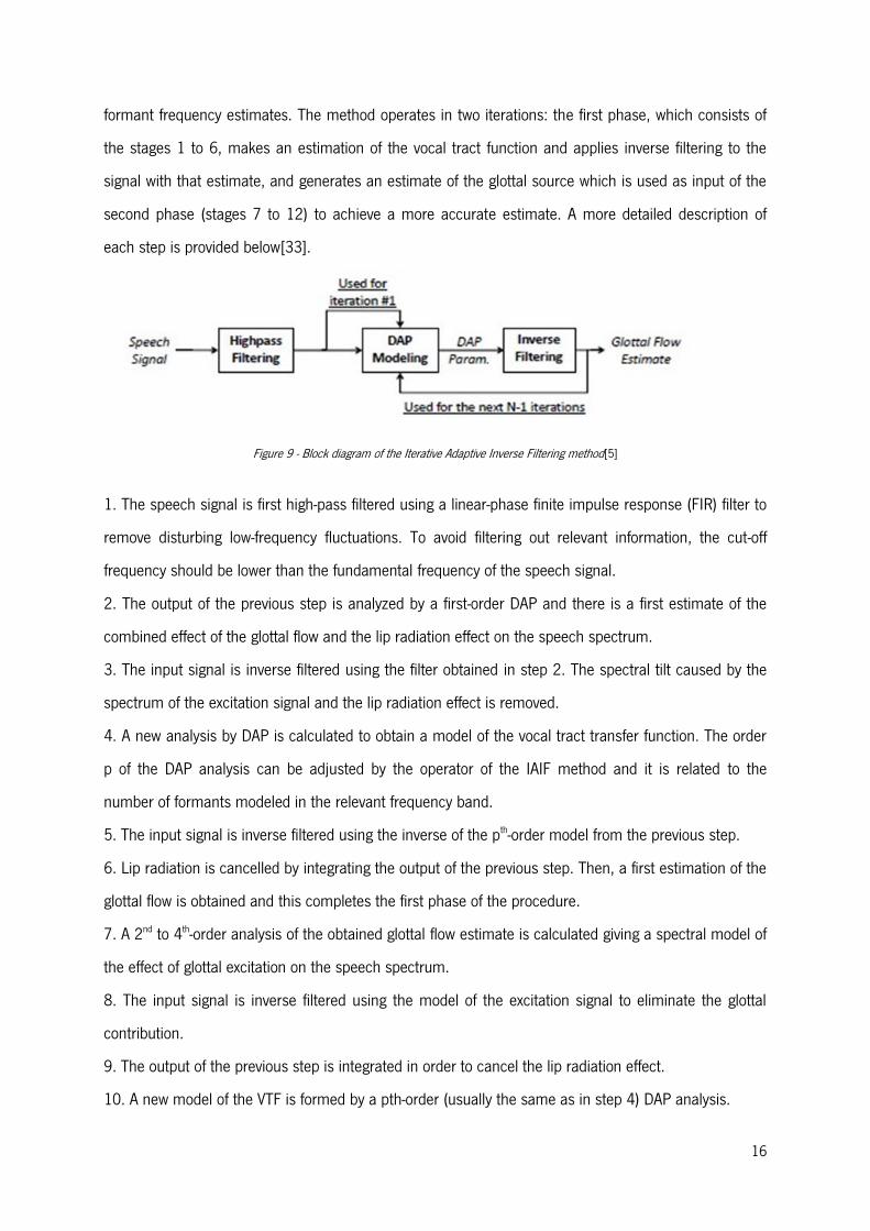
formant frequency estimates. The method operates in two iterations: the first phase, which consists of

the stages 1 to 6, makes an estimation of the vocal tract function and applies inverse filtering to the

signal with that estimate, and generates an estimate of the glottal source which is used as input of the

second phase (stages 7 to 12) to achieve a more accurate estimate. A more detailed description of

each step is provided below[33].

Figure 9 - Block diagram of the Iterative Adaptive Inverse Filtering method[5]

1. The speech signal is first high-pass filtered using a linear-phase finite impulse response (FIR) filter to

remove disturbing low-frequency fluctuations. To avoid filtering out relevant information, the cut-off

frequency should be lower than the fundamental frequency of the speech signal.

2. The output of the previous step is analyzed by a first-order DAP and there is a first estimate of the

combined effect of the glottal flow and the lip radiation effect on the speech spectrum.

3. The input signal is inverse filtered using the filter obtained in step 2. The spectral tilt caused by the

spectrum of the excitation signal and the lip radiation effect is removed.

4. A new analysis by DAP is calculated to obtain a model of the vocal tract transfer function. The order

p of the DAP analysis can be adjusted by the operator of the IAIF method and it is related to the

number of formants modeled in the relevant frequency band.

5. The input signal is inverse filtered using the inverse of the pth-order model from the previous step.

6. Lip radiation is cancelled by integrating the output of the previous step. Then, a first estimation of the

glottal flow is obtained and this completes the first phase of the procedure.

7. A 2nd to 4th-order analysis of the obtained glottal flow estimate is calculated giving a spectral model of

the effect of glottal excitation on the speech spectrum.

8. The input signal is inverse filtered using the model of the excitation signal to eliminate the glottal

contribution.

9. The output of the previous step is integrated in order to cancel the lip radiation effect.

10. A new model of the VTF is formed by a pth-order (usually the same as in step 4) DAP analysis.

17

11. The input signal is then inverse filtered, with the vocal tract model obtained, in order to remove the

effect of the vocal tract.

12. The final estimate of the glottal flow is obtained, removing the lip radiation effect by integrating the

signal.

The output of the Alku’s algorithm are estimations of the glottal flow and the glottal flow derivative.

3.1.2 Complex Cepstrum Decomposition

Homomorphic systems, as the case where inputs are convolved, are important in speech processing.

Separation can be achieved by a linear homomorphic filtering in the complex cepstrum domain, which

presents the property to map time-domain convolution into addition. In speech analysis, complex

cepstrum is usually employed to deconvolve the speech signal into a periodic pulse train and the vocal

system impulse response [34].

The complex cepstrum (CC) ŝ(n) of a discrete signal s(n) is defined by the Discrete-Time Fourier

Transform (DTFT) (Equation 1), the complex logarithm (Equation 2) and the inverse DTFT (IDTFT)

(Equation 3) [35]:

S(ω) = ∑ 𝑠(𝑛)𝑒−𝑗𝜔𝑛∞𝑛=−∞ (1)

log[𝑆(ω)] = log(|𝑆(ω)|) + 𝑗∆𝑆(ω) (2)

ŝ(𝑛) =1

2𝜋∫ log[𝑆(ω)]𝑒𝑗𝜔𝑛 𝑑ω

𝜋

−𝜋 (3)

One difficulty when computing the CC lies in the estimation of ∆S(ω), which requires an efficient phase

unwrapping algorithm. This approach uses the complex cepstrum in order to avoid any factorization.

This decomposition arises from the fact that the complex cepstrum ŝ(n) of an anticausal (causal) signal

is zero for all n positive (negative). Thus, if one considers only the negative part of the CC, it is possible

to estimate the glottal contribution. The CC-based method relies on FFT and IFFT operations offering

the possibility of integrating a causal-anticausal decomposition module into a real-time application,

which was previously almost impossible with the ZZT-based technique. Causal-anticausal decomposition

can be performed using the complex cepstrum (Figure 10), as follows [36]:

1. Window the signal;

2. Compute the complex cepstrum ŝ(n) using Equations 1, 2 and 3;

3. Set ŝ(n) to zero for n > 0;

18

4. Compute ğ(n) by applying the inverse operations of Equations 1, 2 and 3 on the resulting complex

cepstrum.

Figure 10 - Block diagram of the Complex Cepstrum-based decomposition[37].

A simple linear filtering keeping only the negative (or positive) indexes of the complex cepstrum allows

the isolation of the maximum and minimum phase components of voiced speech.

Windowing is known to be a critical issue for obtaining an accurate complex cepstrum and the need of

aligning the window center with the system response is essential [34]. Analysis is performed on

windows centered on the Glottal Closure Instant (GCI), as this particular event defines the boundary

between the causal and anticausal responses and removes the linear phase contribution [38]. However

the window has a considerable effect on the root location in the Z-plane and usual windows (i.e.

Hanning or Hamming) are generally not the best-suited [39]. A window whose duration is about 2 to 3

pitch periods gives a good trade-off for being consistent with the convolutional model [34]. The best

decomposition is achieved for two period-long windows (typically a Hanning-Poisson or Blackman

window).

Many factors may affect the quality of the described decomposition. An obvious assumption, is the

interference between minimum and maximum-phase contributions. The stronger this interference, the

more difficult the decomposition. Basically, this interference is influenced by three parameters:

- The pitch F0, which governs the spacing between two successive vocal system responses;

- The first formant F1, which influences the minimum phase time response;

19

- The glottal formant FG, which controls the maximum-phase time response.

A strong interference then implies a high pitch, with low F1 and FG values. A performance degradation

occurs with the evolution of these factors, equally touching CC and ZZT-based techniques. Also the CC

method suffers from the same noise sensitivity as the ZZT does.

The CC-based method just relies on FFT and IFFT which can be efficiently computed as opposed to the

computational load of the ZZT-based technique which requires to compute the roots of generally high-

order polynomials, despite the accuracy of the current polynomial factoring algorithms. Thus, the

complex cepstrum can be effectively used as a fast alternative to the ZZT algorithm.

3.1.3 Frequency-Domain Glottal Pulse Estimation

In order to analyze and synthesize the glottal source, for a given acoustic signal, the frequency-domain

glottal pulse estimation (FD-GPE) algorithm, which does not depend on GCI localization and that relies

instead on accurate sinusoidal/harmonic analysis and synthesis, characterizes the magnitude and

Normalized Relative Delays (NRDs) of the harmonics (Figure 11). FD-GPE takes advantage of the

spectral diversity between sinusoidal and noise components of voice speech in order to decouple the

phase and magnitude contributions of both source and filter parts of voice production, by also relying

on a model of the glottal pulse (the hybrid Liljencrants-Fant/Rosenberg). This decoupling leads to

incremental accuracy and flexibility since the combination in the frequency domain of the source, filter

and lips/nostrils radiation is multiplicative in the magnitude domain, and additive in the phase or group-

delay domains. One advantage of this approach is that the normalized spectral magnitudes and NRDs

of the harmonics allow to thoroughly define a time waveform shape independently of its fundamental

frequency, time-shift or amplitude, which is essential for a glottal source model. A frequency-domain

analysis-synthesis framework was developed for this approach that includes three main features[40]:

i. The ability to perform accurate signal integration or signal differentiation in the frequency

domain;

ii. The capacity to selectively analyze and resynthesize the harmonic content of a signal modified

or not;

iii. Independent manipulation of both magnitude and phase signal, which makes flexible the

processing of the phase and magnitude contributions acquired from the glottal pulse and vocal

tract filter.

20

Figure 11 – Block diagram of FD-GPE algorithm[41].

Relatively to the glottal flow model, several mathematical models exist, such as the Rosenberg and LF

models (reference models)[42], but their correspondence to physiological data is not clear. For

example, the spectral decay of the LF model (about -16 dB/octave) is significantly higher than the -12

dB/octave reference. This slope reference is usually considered as the natural decay of the glottal pulse

spectrum[42]. Alternatively, the Rosenberg model has a discontinuity in its derivative and, thus, is not a

realistic model. The slope of the linear regression model of the LF model is significantly higher than that

of the Rosenberg model. In fact, the linear approximation for the LF model is given by Equation 4:

𝑦 = 0.0849𝑥 + 0.511 (4)

where x represents the index of the harmonic, for 𝑥 ≥ 2, since by definition the NRD of F0 is always

zero, and for the Rosenberg model is given by Equation 5:

𝑦 = 0.0090𝑥 + 0.2412 (5)

Taking these aspects into consideration, Dias and Ferreira created a hybrid model by using the average

of the normalized magnitudes of the first 24/30 harmonics of each model (LF & Rosenberg), as well as

the corresponding unwrapped NRD coefficients[43]. The different combinations of both linear

regressions were used in order to build an NRD model for the hybrid glottal pulse model. The

smoothest result was obtained for the LF NRD linear model. In fact, the hybrid model is smoother on

the closing phase than the LF and Rosenberg models, nonetheless it reasonably approaches the LF

model while evading the discontinuity on the derivative signal of the Rosenberg glottal model[44].

Regarding the estimation, a region of a voiced sound is first analyzed so as to extract harmonic

information and a smooth spectral envelope model (ceps). Harmonic information includes the

21

frequencies, magnitudes and phases of all sinusoidal components that are harmonics of a fundamental

frequency.

Concerning magnitudes, the magnitude of individual harmonics is first found for each frame of the

source signal, by applying a Sine Window with 1024 samples and using 50% overlap between adjacent

frames at the analysis. Then, for each record the average normalized magnitude of all detected

harmonics (mS) is determined.

A smooth magnitude interpolation of the ceps is determined based on the mS, using the Matlab

function interp1 and a 16-coefficient real cepstrum approach instead of the popular LPC method

because it performs a better match of the poles and the zeros. The smooth envelope is achieved by

“short-pass filtering” the output of ceps.

The dB difference (dBdf) between the magnitude of the spectral peaks and the spectral envelope model

is estimated using Equation 6:

dBdf = mS – ceps (6)

The magnitudes of the glottal source harmonics (mG) (Equation 7) are estimated by adding dBdf to the

magnitude of the spectral peaks of the hybrid glottal model (mGHM):

mG = mGHM + dBdf (7)

Using the frequencies and phases, the NRD coefficients of the voiced speech signal (NRDS) are

determined. In most cases the unwrapped NRDs can be approximated by a line, however its slope is

strongly vowel dependent. Therefore, in order to obtain the linear regression model, the frame where

the highest number of harmonics (up to 30) can be identified is selected. Then, the NRDs of the source

signal (NRDG) are estimated using a compensation function, as follows (Equation 8):

NRDG = NRDS + NRDslope_dif × hind (8)

where NRDslope_dif corresponds to the difference between the slope of the NRDs of the speech signal and

that of the source signal and hind corresponds to the harmonic index. This compensation function

suggests that the acoustic signal delay between the vocal folds and the region outside the lips,

predominates over non-linear phase effects due to the vocal tract filter.

Using the magnitude of the spectral peaks of the glottal model (Equation 7) and the estimated NRDs

(Equation 8), the glottal pulse is synthesized.

22

3.2 Glottal Flow Parameterization

The estimation of the glottal pulse has usually a final step consisting in the parameterization, whose

purpose is to determine quantitative features of the signal that characterize the glottal wave and may

quantify a perception parameter[45]. Once the glottal flow waveform has been estimated it can be

parameterized by expressing its most important properties in a compressed numerical form.

Parameterization of the time-domain glottal flow signals can be computed using time-based or

amplitude-based methods. In the former, the most straightforward classical method is to compute time

duration ratios between different phases of the glottal flow pulse[46]. Thus, the flow pulse is separated

into three parts (Figure 12): the closed phase (Tc), the opening phase (To), and the closing phase (Tcl).

Figure 12 - The flow pulse phases

The most widely used time-based parameters are defined as follows: open quotient (Equation 9), speed

quotient (Equation 10), and closing quotient (Equation 11),

𝑂𝑄 = (𝑇𝑜 + 𝑇𝑐𝑙) 𝑇⁄ (9)

𝑆𝑄 = 𝑇𝑜 𝑇𝑐𝑙⁄ (10)

𝐶𝑙𝑄 = 𝑇𝑐𝑙 𝑇⁄ (11)

where the length of the fundamental period is denoted by Equation 12:

𝑇 = 𝑇𝑐 + 𝑇𝑜 + 𝑇𝑐𝑙 (12)

Time-based measures are vulnerable to distortions in the glottal flow waveforms due to incomplete

cancelling of formants by the inverse filter, reducing the precision and robustness of these parameters.

Therefore, computation of the time-based parameters is sometimes performed by replacing the true

opening and closure instants by the time instants when the glottal flow crosses a level which is set to a

23

given value between the minimum and maximum amplitude of the glottal cycle. The Quasi-Open

Quotient (QOQ), defined as the ratio between the quasi-open time and the quasi-closed time of the

glottis, and corresponds to the timespan (normalized to the pitch period) during which the glottal flow is

above 50% of the difference between the maximum and minimum flow. It was proposed as a parameter

describing the relative open time of the glottis. The quasi-open phase is the duration between time

instants prior to and following the maximum amplitude of the glottal flow that descend below 50% of

this peak amplitude[47].

Time-based features of the glottal source can be quantified by measuring the amplitude-domain values

of the glottal flow and its derivative[48]. Amplitude-based measures were first used in the

parameterization of the voice source by Gobl and Chasaide whom proposed methods to express three

LF-based parameters (glottal frequency, skew parameter, and open quotient) in terms of amplitude-

based measures[49].

The computation of the Normalized Amplitude Quotient (NAQ) is done from two amplitude values: the

AC-amplitude of the flow (noted fAC) and the negative peak amplitude (dmin) of the glottal flow derivative

(Equation 13)[50].

𝑁𝐴𝑄 = 𝑓𝐴𝐶 𝑑𝑚𝑖𝑛 ∙ 𝑇⁄ (13)

Since these two amplitude measures are the largest values of the flow and can be found in every glottal

cycle, it is straightforward to extract them even when the estimated glottal sources are distorted.

Another parameter called the waveform peak factor (WPF), which measures the decay characteristics of

a speech waveform during a single pitch period, was proposed by Wendahl in 1963. The WPF value of

a speech waveform with narrow pulses and separated by a long glottal closure is large and for pulses of

long duration the WPF is near unity[51].

When GIF is computed with the flow mask of Rothenberg it is possible to parameterize the amplitude-

based properties of the time-domain waveforms of the glottal flow and its derivative. The most widely

used amplitude parameters are the minimum flow (also called the DC-offset), the AC-flow and the

negative peak amplitude of the flow derivative. The ratio between the AC and DC information has been

used in the amplitude-based quantification of the glottal source. It is also possible to parameterize the

time-domain voice source by searching for a model waveform that matches the estimated glottal

excitation (or its derivative)[52]. Time-domain reproduction of the glottal excitation estimated by inverse

filtering is also possible by searching for the physical parameters (e.g. vocal fold mass and stiffness) of

24

the underlying oscillator rather than through explanation of the waveform of the volume velocity

signal[53].

In Gudnason et al. [3] a data-driven approach was developed for glottal flow estimation, and was first

computed with IAIF and the obtained waveform was then processed with Principal Component Analysis

(PCA) in order to achieve dimensionality reduction. The first few PCA components were then modelled

with Gaussian Mixture Models (GMMs). GMMs are a generative learning algorithm which involve

modelling a given class of data using a mixture of multi-variate Gaussians[47]. The obtained GMMs

were shown to enable parameterizing source features, such as non-flatness of the closed phase that

traditional approaches fail to model[3]. Artificial Neural Networks (ANNs) are in general used for

learning the mapping function ƒ from I to T as detailed in [47]. Another classification algorithm used in

the mentioned work was Support Vector Machines (SVMs). SVMs in general look to find a separating

hyperplane which maximizes the functional margin between two classes. Techniques also exist to

extend the binary classification capability to more than two classes. A different automatic

parameterization method of the voice source is based on simulating the strategies that are used in

manual optimization of the LF parameters. The technique proposed has three main parts. First, an

exhaustive search is executed to get a group of most suitable parameter settings. A dynamic

programming algorithm is then used to select the best path of the parameter values by considering two

costs (target and transition) in the parameter trajectories of the modeled glottal pulses. As the final part,

an optimization method is employed to refine the fit[54].

Frequency domain parameterization of the glottal source has been computed by measuring the spectral

skewness with the so called alpha ratio, which is the ratio between spectral energies below and above a

certain frequency limit (typically 1.0 kHz) that quantify the spectral slope of the glottal source by

utilizing the level of the fundamental frequency and its harmonics. Obtaining the spectrum pitch

synchronously opens up the possibility of taking a variety of spectral measurements specifically related

to glottal flow characteristics and perturbations. We may give as examples the average percentage

amplitude perturbation for the first harmonic named APAP, the distortion factor (amplitude of F0 divided

by total signal amplitude) and the H1–A3, that measures the amplitude of the 1st harmonic to that of

the first formant frequency[55]. The harmonic richness factor (HRF), proposed by Childers and Lee, is

defined for the spectrum of the estimated glottal flow as the ratio of the sum of the amplitude of the

higher harmonics and the 1st harmonic[51]. In addition, levels of spectral harmonics have been used in

the parameterization of the glottal flow to measure the decay of the voice source spectrum by

25

performing linear regression analysis over the first eight harmonics[56]. Analysis of the spectral slope of

the voice source of singers by computing the difference, denoted by H1-H2, between the amplitude of

the fundamental and the second harmonic was attempted by Titze and Sundberg[57]. A similar

measure of the spectral tilt is computed directly from the radiated speech signal by correcting the

effects of vocal tract filtering without computing the glottal flow by GIF. Alku introduced, in 1997, a

frequency domain method based on fitting a low-order polynomial in the pitch synchronous source

spectrum[58]. Parabolic spectrum parameter (PSP) is another frequency-domain parameter, which fits

a second-order polynomial to the flow spectrum to gain an estimate of the spectral slope[59].

Also, it is possible to quantify the glottal excitation by measuring the ratio between the harmonic and

non-harmonic components, especially in the analysis of disordered voices, in which the glottal excitation

typically involves an increasing amount of aperiodicities due to jitter, shimmer, aspiration noise, and

modifications in the pulse waveform[55].

3.3 Applicability in Biomedical Applications

At the crossroads between biomedical engineering and signal processing, glottal source processing has

been demonstrated to be useful in several health-related applications. Its most direct application is for

voice disorder detection. Speech pathologies are frequently associated with a dysfunction of the vocal

folds, as an edema, or a polyp or nodule.

Features used to define the glottal behavior are therefore of great importance for the automatic audio-

based detection of voice pathologies. Two of these measures, jitter and shimmer, are parametrized to

characterize anomalies in a quasi-periodic signal[60]. Jitter refers to the variation in the duration of

consecutive glottal cycles, while shimmer reflects the alterations in amplitude of consecutive glottal

cycles. Different methods to estimate the amount of jitter in speech signals with an objective on their

ability to detect pathological voices are known. Short-term jitter estimates are best provided by the

spectral jitter estimator (SJE), which is centered on a mathematical description of the jitter

phenomenon[61]. SJE was proposed in order to analyze continuous speech. The jitter values obtained

were able to confirm studies presenting a decrease of jitter with increasing fundamental frequencies, as

well as a more frequent presence of high jitter values in the pathological voices. A variant of the

traditional Harmonic-to-Noise Ratio (HNR) measure, called glottal-related HNR (GHNR’), was proposed

to overcome the F0 dependency denoted in the usual HNR formulation[62]. For voice pathology

26

discrimination, GHNR’ is shown to provide statistically significant differentiating supremacy over a

conventional HNR estimator. The use of the glottal source estimation to detect voice disorders show

that speech and glottal-based features are relatively complementary, despite some synergy with

prosodic characteristics[63]. The combination of glottal and speech-based features offers higher

discrimination capacities. The phase information, generally associated with the glottal production, is

shown to be appropriate to highpoint irregularities in phonation when compared to its magnitude

equivalent.

The use of glottal source processing in medical applications is not only restricted to pathological voices

as the technologies developed can also be applied to examine healthy voices in danger of becoming

disordered due to vocal loading[64]. Vocal loading refers to extended usage of voice in association with

environmental factors such as background noise and/or poor air quality[65]. Since the number of

employees in the voice-intensive occupations has been increasing, the work-related voice care will

become a progressively essential application area for glottal source processing.

Glottal characterization has also been helpful with the classification of clinical depression in speech

since the vocal jitter and glottal flow spectrum were proposed as possible indications of a patient’s risk

of committing suicide[66]. Three groups were considered: high-risk near-term suicidal patients, major

depressed patients, and non-depressed control subjects. The mean vocal jitter was found to be a

significant discriminator between suicidal and non-depressed control groups, while the slope of the

glottal flow spectrum shown a substantial discriminating capacity among all three groups.

Discriminating depressed speech from normal speech was also analyzed and it showed that the

combination of glottal and prosodic features produces enhanced discrimination over the combination of

prosodic and vocal tract features[67]. It is also emphasized that glottal features are essential

components of vocal affect analysis. Towards the goal of objective observation of depression severity,

vocal-source biomarkers for depression were considered[68]. These biomarkers are specifically source

features and their results highlight the statistical associations of these vocal-source biomarkers with

psychomotor activity and depression severity. Using an Auto-Regressive eXogenous (ARX) model

combined with the LF model, a human voice can be classified as joy, anger, neutral or sad speech,

which facilitates a psychological evaluation of patients. For joy speech and anger speech, the shape of

glottal flow looks like triangular wave, a result that fits with the human speech production mechanism

when in excited state. In the production of joy and anger speech, the glottis has high pressure and the

glottal folds vibrate more quickly. For sad speech the shape of glottal flow is smoother because air flow

27

arrives slowly at the vocal folds which makes the glottal folds open slowly when humans are in a sad

state. Also, the high frequency energy of joy and anger speech is higher than neutral speech, and sad

speech’s is the lowest[69].

The use of the glottal source can also be useful in applications for laryngectomees. Patients having

undergone total laryngectomy cannot produce speech sounds in the orthodox method since their vocal

folds have been removed. Allowing patients to regain voice is then the major goal of the post-surgery

process. Several approaches aimed the resynthesis of an enriched form of alaryngeal speech, in order

to develop its quality and intelligibility. For this purpose, generation of an artificial excitation signal

based on the understanding of glottal production is necessary. For example, Qi, Weinberg and Bi [70]

have concluded that analyzing resynthesized female alaryngeal words with a synthetic glottal waveform

and with smoothed and raised F0 showed that the replacement of the glottal waveform and F0

smoothing alone produces the most significant enhancement, while increasing the average F0 leads to

less dramatic improvement. A speech repair system, that resynthesizes alaryngeal speech using a

synthetic glottal waveform, reduces jitter and shimmer and applies a spectral smoothing and a tilt

correction algorithm along with a reduction of the perceived breathiness and harshness of the

voice[71].

Dysphonia measures (similar to those used for voice pathology evaluation) were shown to outperform

previous results in the detection of Parkinson’s disease (PD)[72]. These features complement existing

algorithms in maximizing the capability to distinguish healthy controls from PD subjects and represent a

promising step toward the early non-invasive diagnostic of PD.

29

4. EXPERIMENTAL TESTS

Most of the techniques for the estimation of the glottal source are based on the source-filter model and,

thus, have a model for the vocal tract transfer function in order to eliminate the effect of the vocal tract

filter and to cancel the lip/nostrils radiation from the speech signal. In the literature, most often, the

vocal tract filter is modelled as an all-pole filter that shapes the spectrum of the source according to the

resonances of the vocal tract, and the lip/nostrils radiation is typically modelled as a first-order discrete-

time derivative operator of the pressure wave at the output of vocal tract. This operation converts

volume velocity of the air flow into sound pressure variation, the physical quantity captured by a

microphone. Thus, the glottal pulse inverse filtering requires a first-order integration operation in order

to eliminate the lip/nostrils radiation from the speech signal. Most of the inverse filtering techniques

implement this operation in time domain (e.g., IAIF), but it motivates two sources or approximation

errors: a first error is due to the first-order differentiator, since the frequency response clearly differs

from the frequency response of an ideal differentiator, especially at high frequencies; a second error is

due to the inverse transfer function of the first-order differentiator, in order to avoid the pole at z =1 and

to insure stability. This is achieved by moving the pole slightly away from Z=1 (in order to insure

stability) and by affecting the gain, a typical difference equation of such an approximate integrator is

represented by Equation 14,

𝑦[𝑛] = (1 − 𝛼)𝑥[𝑛] + 𝛼 × 𝑦[𝑛 − 1] (14)

where α is a positive constant less than the unity.

For this experience some assumptions were made:

• 2 adult volunteer subjects participated, one of each gender;

• All subjects have healthy voices, i.e., no voice disorders;

• The subjects uttered (the back and front) common Portuguese vowels “a” and “i”.

The choice of the sustained vowels “a” and “i” was because they represent a relatively stable condition

of the phonatory system and there is a minor vocal tract influence in their glottal source[73].

The original recording sampling frequency was 22050 Hz in order to facilitate subsequent processing,

namely in terms of spectral analysis.

In this section the new approach to speech filtering for glottal source estimation, described previously,

is tested with twelve speech signals including eight synthetic and four real. The results from three

30

algorithms, two main state-of-the-art methods (IAIF and CCD) and the recently developed FD-GPE, are

evaluated and compared.

It should be noted that the CCD only delivers the estimation of the glottal source derivative (and the

estimation of the vocal tract filter). Although we could implement the integration step in order to achieve

the glottal source signal, it would be a modification of the result of the original procedure. Therefore, in

this section, the estimations of the glottal source derivative using the CC decomposition will be

presented, will be compared to the ones obtained using IAIF (that are not necessarily results of

reference) and will only be evaluated qualitatively.

In order to assess the quality of the estimations, the evaluation of the estimations using IAIF and FD-

GPE will be complemented with an objective quantitative measure, the Signal to Noise Ratio (SNR),

which compares the signal and the noise resulting from the difference between the estimated and the

reference signal, and efficient glottal flow estimations are then reflected in higher SNR values.

According to the definition of SNR, this value is only computed when the glottal source signal is known,

as it happens in the case of synthetic signals.

4.1 Tests with Synthetic Speech Signals

Eight synthetic signals will be used in order to compare and evaluate the estimations of the glottal

source: one of each gender, normal and derived, for vowels “a” and “i”. These signals were generated

using the Matlab toolbox Voicebox, with the derivative of the LF model used as glottal impulse, and an

all-pole filter extracted by LPC analysis of real sustained vowels from real male and female speech

signals as the synthesized VTF. The fundamental frequency was 110 Hz and 220 Hz, for the male and

the female synthetic signals, respectively. The IIR filter, utilized in this work, uses an 18th order LPC

method to synthesize the vocal tract in resemblance to the voices of the female and male volunteers.

The generated filter is applied to the LF derived glottal impulse, which is then normalized. The next step

is to pass the resulting speech signals through a linear-phase FIR filter (the Parks-McClellan algorithm,

explained in section 4.1.1) of 500th order with the same frequency response of the IIR filter and also

with the coefficients extracted from the LPC method with a posterior normalization of the signal.

Therefore, our tests include four signals which are generated using the traditional IIR filter as a model

for the VTF, and four signals which are generated using the same glottal excitation but using a linear-

phase FIR filter having the same magnitude response of the IIR filter, as VTF model.

31

The resulting signals will be subjected to the selected estimation algorithms and measured with SNR to

evaluate the differences between the two filtering approaches and to determine the best algorithm for

the new test condition.

4.1.1 Parks-McClellan Algorithm

A linear-phase filter is typically used when a causal filter is needed to modify a signal's magnitude-

spectrum while preserving the signal's time-domain waveform as much as possible. In signal

processing, a FIR filter is a filter whose impulse response (to any finite length input) is of finite duration,

because it settles to zero in finite time. A FIR filter is linear-phase if (and only if) its coefficients are

symmetrical around the center coefficient (having an odd number of coefficients, it will have a single

coefficient in the center with no mate). Given a FIR filter which has N taps, the delay can be calculated

by Equation 15:

(𝑁−1)

(2×Fs), (15)

where Fs is the sampling frequency.

The Parks–McClellan algorithm, published by Thomas Parks and James McClellan in 1972, is an

iterative algorithm for finding the optimal Chebyshev finite impulse response (FIR) filter. The Parks-

McClellan algorithm uses the Remez exchange algorithm and Chebyshev approximation theory to

design filters with an optimal fit between the desired and actual frequency responses. The filters are

optimal in the sense that the maximum error between the desired frequency response and the actual

frequency response is minimized through the minimization of the error in the pass and stop bands by

utilizing the Chebyshev approximation. It has become a standard method for FIR filter design. Filters

designed this way exhibit an equiripple behavior in their frequency responses and are sometimes called

equiripple filters.

4.2 Tests with Real Speech Signals

Following the tests using synthetic signals, eight real signals will be tested. Four real signals will be

used with the natural conditions and the others four will be subjected to the FIR filer in order to

compare and evaluate the estimations of the glottal source: one of each gender, normal phonation, for

vowels “a” and “i”:

• A female vowel “a” with F0=372 Hz;

32

• A female vowel “i” with F0=464 Hz;

• A male vowel “a” with F0=261 Hz;

• A male vowel “i” with F0=266 Hz.

The reference signals for the real voice samples were captured by a microphone as close as possible to

the vocal folds[43], and therefore, a better evaluation is possible for the estimations provided by the

different algorithms.

33

5. RESULTS & DISCUSSION

In this section, we will describe the generated speech signals after VTF filtering and the results of the

glottal pulse estimation by the three already mentioned algorithms. The SNR measurement was only

calculated for the IAIF and FD-GPE algorithms because the latter method does not provide a glottal flow

derivative, which is the only output of the complex cepstrum based decomposition.

5.1 Synthetic Speech Signals

In order to perform a correct analysis of the effect of both filters, the Parks-McClellan filter and the all-

pole filter must have the same magnitude frequency response and design, despite being of different

order.

A consequence of the FIR filter is the constant delay the filter introduces to the speech signal, which is

far superior than the delay due to the IIR filter and that depends on the frequency as displayed in Figure

13 for female signals and Figure 14 for male signals. Another difference concerning both types of filters

is that the FIR filter presents ripple in its magnitude frequency response which is a natural consequence

of the design method. Figure 15 and Figure 16 show the design of these filters from both vowels in the

female and in the male synthesized voices, respectively.

34

Figure 13 – Group delay of the synthesized female signals. a) Represents the filters’ design for vowel “a”. b) Represents the filters’ design for vowel “i”.

35

Figure 14 – Group delay of the synthesized male signals. a) Represents the filters’ design for vowel “a”. b) Represents the filters’ design for vowel “i”

After all the synthetic speech sequences have been generated, the estimation of the glottal flow was

performed using the IAIF, CCD and FD-GPE algorithms. Figures 17 to 24 present the estimations and

the original speech signal, enabling the visual analysis of the different results delivered by the three

algorithms.

36

Figure 15 – Frequency magnitude response of the female synthesized speech. a) Represents the filters’ design for vowel “a”. b) Represents the filters’ design for vowel “i”.

The estimations of the glottal pulse derivative, using the CCD algorithm, noticeably approaches the LF

glottal flow derivative waveform, except from the minimum, where the estimations are significantly

smoother. This implies that the corresponding glottal pulses would not have the abrupt closure as the

LF glottal model. Also, it is noticeable that this estimation method is less effective among the female

signals, which corroborates that the CC decomposition efficiency reduces significantly in high frequency

signals.

37

Figure 16 – Frequency magnitude response of the male synthesized speech. a) Represents the filters’ design for vowel “a”. b) Represents the filters’ design for vowel “i”.

Moreover, the FIR filtered signals displays an estimation that better resembles the LF glottal flow

derivative.

When comparing the estimations performed by CCD to the glottal flow derivatives estimated using IAIF,

the differences are obvious, in particular the presence of ripples displayed in the IAIF results, giving to

the former method a clearly better performance in these signals.

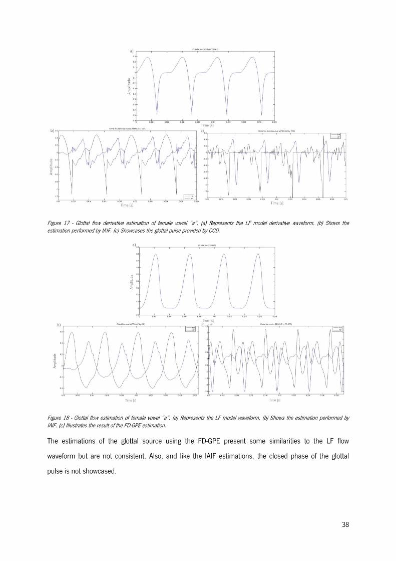
38

Figure 17 - Glottal flow derivative estimation of female vowel “a”. (a) Represents the LF model derivative waveform. (b) Shows the estimation performed by IAIF. (c) Showcases the glottal pulse provided by CCD.

Figure 18 - Glottal flow estimation of female vowel “a”. (a) Represents the LF model waveform. (b) Shows the estimation performed by IAIF. (c) Illustrates the result of the FD-GPE estimation.

The estimations of the glottal source using the FD-GPE present some similarities to the LF flow

waveform but are not consistent. Also, and like the IAIF estimations, the closed phase of the glottal

pulse is not showcased.

39

Figure 19 - Glottal flow derivative estimation of female vowel “i”. (a) Represents the LF model derivative waveform. (b) Shows the estimation performed by IAIF. (c) Showcases the glottal pulse provided by CCD.

Figure 20 - Glottal flow estimation of female vowel “i”. (a) Represents the LF model waveform. (b) Shows the estimation performed by IAIF. (c) Illustrates the result of the FD-GPE estimation.

While the glottal flow estimations provided by IAIF are relatively similar between vowels and for the

same gender, the results of the FD-GPE algorithm are significantly different for gender and in the female

estimations are also distinct between vowels.

40

Figure 21 - Glottal flow derivative estimation of male vowel “a”. (a) Represents the LF model derivative waveform. (b) Shows the estimation performed by IAIF. (c) Showcases the glottal pulse provided by CCD.

Figure 22 - Glottal flow estimation of male vowel “a”. (a) Represents the LF model waveform. (b) Shows the estimation performed by IAIF. (c) Illustrates the result of the FD-GPE estimation.

41

Figure 23 - Glottal flow derivative estimation of male vowel “i”. (a) Represents the LF model derivative waveform. (b) Shows the estimation performed by IAIF. (c) Showcases the glottal pulse provided by CCD.

Figure 24 - Glottal flow estimation of male vowel “i”. (a) Represents the LF model waveform. (b) Shows the estimation performed by IAIF. (c) Illustrates the result of the FD-GPE estimation.

The assumptions extracted from visualization, were validated by the SNR measurement as shown in

Table 1. SNR application was performed after signal alignment and scale matching between the

estimated signal and the LF model of the glottal pulse, in order to establish the minimum difference.

42

Table 1 – SNR results for all the estimated glottal flows for the IAIF algorithm and the FD-GPE algorithm.

Female FIR

vowel “a”

Female IIR

vowel “a”

Female FIR

vowel “i”

Female IIR

vowel “i”

Male FIR

vowel “a”

Male IIR

vowel “a”

Male FIR

vowel “i”

Male IIR

vowel “i”

IAIF 12.0809 15.4320 10.1830 10.2774 15.9098 15.9342 15.970 16.2217

FD-GPE 13.1716 14.4153 14.4794 15.0715 11.3093 6.5707 12.1188 8.0529

Analyzing the filters, for the IAIF algorithm, all the signals performed better without the Parks-McClellan

filter over the LPC filter. An explanation for this is the fact that the LPC filter is encoded in the IAIF

algorithm. The estimations provided by the FD-GPE algorithm reveal significant enhanced results in the

FIR filtered signals of both male vowels when comparing the filtering methods.

Comparing both algorithms, with the all-pole filter, IAIF is the best algorithm for all the signals except for

the female vowel “i”, while with the FIR method, FD-GPE presents the best SNR measures for female

vowels and IAIF for the male estimations.

A possible explanation for a superior performance of the IAIF algorithm in these tests is the fact that the

signals were synthesized based on the LF waveform model and the FD-GPE algorithm shapes the glottal

flow estimation on the hybrid LF-Rosenberg model.

5.2 Real Speech Signals

Following the tests with the synthetic signals, we consider now the estimation results using real human

voice signals as inputs to the algorithms. The Figures 25 to 28 present the estimations in the

mentioned conditions, enabling the visual analysis of the different algorithms. It is important to mention

that, since a derivative of the two subjects’ glottal flow is not available, the CCD estimation will only be

visually compared to the CCD estimation of the synthetic signals.

Concerning the estimations performed by the CCD algorithm for the same signals, they quite

approximate classic glottal pulse derivative models, except on the closing phase, in which the FIR

filtered estimations showcase the best waveform shape while being consistent along the signal periods.

This is the case for both genders and for each vowel uttered, however the results performed by CC

decomposition do not allow substantial conclusions since this method only gives the glottal source

derivative estimation.

43

Similarities between the glottal source estimations using IAIF and FD-GPE can be noted. The

estimations performed by these two methods show the classic asymmetry and bell-shape of the glottal

pulse, often mentioned in the literature.

Figure 25 - Glottal flow estimation of the female subject vowel “a”. (a) Represents the female glottal pulse waveform extracted. (b) Shows the estimation performed by CCD. (c) Showcases the estimation performed by IAIF. (d) Illustrates the result of the FD-GPE estimation.

An important and common feature of most of these glottal flow estimations is the shape of the

waveform on the closing phase.

Figure 26 - Glottal flow estimation of the woman’s vowel “i”. (a) Represents the woman glottal pulse waveform extracted. (b) Shows the estimation performed by CCD. (c) Showcases the estimation performed by IAIF. (d) Illustrates the result of the FD-GPE estimation.

44

It is clear that the glottal flow estimations provided by the FD-GPE algorithm are, in portions, identical to

the waveforms of the corresponding signals captured near the glottis.

Figure 27 - Glottal flow estimation of male subject vowel “a”. (a) Represents the male glottal pulse waveform extracted. (b) Shows the estimation performed by CCD. (c) Showcases the estimation performed by IAIF. (d) Illustrates the result of the FD-GPE estimation.

Figure 28 - Glottal flow estimation of the man’s vowel “i”. (a) Represents the male glottal pulse waveform extracted. (b) Shows the estimation performed by CCD. (c) Showcases the estimation performed by IAIF. (d) Illustrates the result of the FD-GPE estimation.

45

For the woman’s estimations, FD-GPE performs, visually, the best for vowel ‘a’ with the FIR filter while

the IIR filtered signal estimation is more accurate to the vowel ‘i’ reference signal. As for the opposite

gender, the estimations with the IIR filter are the most similar to the reference signals for each vowel. It

is to be noted that the Parks-McClellan filtered vowel ‘a’ showcases what appears to be an inversion of

the signal peak, therefore the best visual performance by LPC filtered signal. All the real estimations are

robust between periods.

As for the IAIF algorithm, the real female estimations for both vowels better resemble the theoretical

waveform shape of the glottal flow than the reference signals. Visually, the IIR filtered signal estimations

are the best, even with the slight oscillations for the vowel ‘a’. Regarding the man’s estimations, the

waveform shape is also less resembling to the reference signal shaped than desired. However, in these

gender’s estimations the FIR filtered signals are the ones with the best visual match to each of the

vowels’ reference signals.

The assumptions extracted from visualization, were validated by the SNR measurement as shown in

Table 2. SNR application was performed after signal alignment and a scaled match between the signal

estimated and the reference signals obtained as described in Section 4.2.

Table 2 – SNR results for all the estimated glottal flows for the IAIF algorithm and the FD-GPE algorithm for human speech.

Woman

FIR vowel “a”

Woman IIR vowel

“a”

Woman FIR vowel

“i”

Woman IIR vowel

“i”

Man FIR vowel “a”

Man IIR vowel “a”

Man FIR vowel “i”

Man IIR vowel “i”

IAIF 1.8162 2.5322 3.1904 3.9234 6.1630 5.3994 6.5356 6.0291

FD-GPE 4.9482 4.0907 1.4857 3.0875 6.6195 7.0538 5.0869 5.0956 Analyzing the filtering methods, for the IAIF algorithm, both the man vowels performed better with the

Parks-McClellan filter over the IIR filter. The estimation provided by the FD-GPE algorithm reveals

boosted results in the FIR filtered signal for only the vowel “a” of the feminine subject.

Comparing both algorithms, IAIF is the best algorithm for both genders vowel “i” with both filters while

FD-GPE presents the best SNR measures for both genders vowel “a”.

46

47

6. CONCLUSION

In recent years, the estimation of the glottal pulse from a speech signal raised the interest of many

researchers due to its great potential in speech science, namely the medical applications. Despite the

concealed location of the vocal folds and the difficulties on capturing directly and non-invasively the

glottal source signal, computational alternatives have been proposed over the years in order to

accurately estimate the glottal source directly from speech signals. Most of the glottal source estimation

procedures are based on the source-filter model in which the glottal source is estimated by extracting

both the glottal source and the vocal tract filter from a recorded voice signal. These are then separated

in order to obtain the glottal flow generated at the glottis.

In this dissertation a new filtering approach to glottal source estimation was proposed, using a filter

based on the Parks–McClellan algorithm which is shaped by the frequency response and coefficients of

an 18th-order LPC filter of the voice sample to be studied. The performance of the mentioned approach

has been evaluated and compared on eight speech signals, synthetic and real, using three algorithms

FD-GPE, IAIF and CCD been the last two representative state-of-the-art techniques. In order to assess

the quality of the glottal source estimations, the SNR objective measure was used.

The results have shown that for synthetic signals, the estimations provided by the FD-GPE algorithm

reveal significant enhanced results in the FIR filtered signals of both male vowels and presents the best

SNR measures for the female glottal flow estimations. For real signals, the IAIF algorithm performed

better with the Parks-McClellan filter for both male vowels over the all-pole filter. The estimation

provided by the FD-GPE algorithm reveals enhanced results for the vowel “a” of the feminine subject

when filtered with the Parks-McClellan filter instead of with the LPC filter. FD-GPE presents the best SNR

measures for both genders vowel “a” with both filtering methods when compared to the IAIF algorithm.

Visually, all the CCD algorithm estimations are improved by the FIR filtered signals both in synthetic and

real tests.

A possible improvement for the proposed approach is to shape the FIR filter based on a DAP filter

instead of a LPC filter since the peaks of linear prediction spectral estimates are highly biased towards

the pitch harmonics, for high-pitched voices which is the case of female voices.

The developed filtering approach exhibits promising results, which will result in its implementation in

the FD-GPE algorithm.

48

49

BIBLIOGRAPHY

[1] J. Flanagan, Speech analysis: Synthesis and perception, 2nd Editio. Springer-Verlag, 1972.

[2] T. Drugman, P. Alku, A. Alwan, and B. Yegnanarayana, “Glottal source processing: From analysis to applications,” Comput. Speech Lang., vol. 28, no. 5, pp. 1117–1138, Sep. 2014.

[3] J. Gudnason, M. R. P. Thomas, D. P. W. Ellis, and P. a. Naylor, “Data-driven voice source waveform analysis and synthesis,” Speech Commun., vol. 54, pp. 199–211, Feb. 2012.

[4] K. Tokuda, T. Kobayashi, T. Masuko, and S. Imai, “Mel-Generalized Cepstral Analysis: A Unified Approach to Speech Spectral Estimation.,” in Proceedings of 1994 International Conference on Spoken Language Processing, 1994, no. 2, pp. 1043–46.

[5] T. Drugman, “Advances in glottal analysis and its applications,” University of Mons, 2011.

[6] J. Seikel, D. King, and D. Drumright, Anatomy & physiology for speech, language, and hearing, 4th Editio. Delmar Cengage Learning, 2010.

[7] J. Sundberg, The science of singing voice. Dekalb, Illinois: Northern Illinois University Press, 1987.

[8] K. Murphy, “Digital Signal Processing Techniques for Application in the Analysis of Pathological Voice and Normophonic Singing Voice,” Universidad Politécnica de Madrid, 2008.

[9] F. Pereira, Comunicações Audiovisuais: Tecnologias, Normas e Aplicações. Lisboa: Instituto Superior Técnico, 2009.

[10] R. Goldberg and L. Riek, A Practical Handbook of Speech Coders. CRC Press, 2000.

[11] G. P. Kafentzis, “On the glottal flow derivative waveform and its properties,” University of Crete, 2008.

[12] A. Ó. Cinnéide, “PhD Tranfer Report,” Dublin, 2008.

[13] R. L. Miller, “Nature of the Vocal Cord Wave,” J. Acoust. Soc. Am., vol. 31, no. 6, pp. 667–677, Jun. 1959.

[14] A. Oppenheim and R. Schafer, “Homomorphic analysis of speech,” IEEE Trans. Audio Electroacoust., vol. 16, no. 2, pp. 221–226, 1968.

[15] M. Nakatsui and J. Suzuki, “Method of Observation of Glottal-Source Wave Using Digital Inverse Filtering in Time Domain,” J. Acoust. Soc. Am., vol. 47, no. 2, pp. 2–3, 1970.

[16] M. Rothenberg, “A new inverse-filtering technique for deriving the glottal air flow waveform during voicing,” J. Acoust. Soc. Am., vol. 53, no. 6, pp. 1632–1645, 1973.

50

[17] M. Rothenberg, “Measurement of airflow in speech,” J. Speech Hear. Res., vol. 20, pp. 155–176, 1977.

[18] M. Rothenberg and S. Zahorian, “Nonlinear inverse filtering technique for estimating the glottal-area waveform,” J. Acoust. Soc. Am., vol. 61, no. 4, pp. 1–19, 1977.

[19] S. Granqvist, “Simultaneous analysis of vocal fold vibration and transglottal airflow ; Exploring a new experimental set-up,” TMH-QPSR, vol. 45, pp. 35–46, 2003.

[20] H. Strube, “Determination of the instant of glottal closure from the speech wave,” J. Acoust. Soc. Am., vol. 56, no. 5, pp. 1625–1629, 1974.

[21] A. Krishnamurthy and D. Childers, “Two-channel speech analysis,” IEEE Trans. Acoust. Speech Signal Process., vol. 34, no. 4, pp. 730–43, 1986.

[22] B. Yegnanarayana and R. Veldhuis, “Extraction of vocal-tract system characteristics from speech signals,” IEEE Trans. Speech Audio Process., vol. 6, no. 4, pp. 313–327, 1998.

[23] O. O. Akande and P. J. Murphy, “Estimation of the vocal tract transfer function with application to glottal wave analysis,” Speech Commun., vol. 46, no. 1, pp. 15–36, May 2005.

[24] P. Alku, C. Magi, S. Yrttiaho, T. Bäckström, and B. Story, “Closed phase covariance analysis based on constrained linear prediction for glottal inverse filtering,” J. Acoust. Soc. Am., vol. 125, no. 5, pp. 3289–305, May 2009.

[25] P. Milenkovic, “Glottal inverse filtering by joint estimation of an AR system with a linear input model,” IEEE Trans. Acoust. Speech Signal Process., vol. 34, no. 1, pp. 28–42, 1986.

[26] Q. Fu and P. Murphy, “Robust glottal source estimation based on joint source-filter model optimization,” IEEE Trans. Acoust. Speech Lang. Process., vol. 14, no. 2, pp. 492–501, 2006.

[27] B. Bozkurt and B. Doval, “Zeros of z-transform representation with application to source-filter separation in speech,” IEEE Signal Process. Lett., vol. 12, no. 4, pp. 344–347, 2005.

[28] G. Degottex, A. Roebel, and X. Rodet, “Phase minimization for glottal model estimation,” IEEE Trans. Acoust. Speech Lang. Process., vol. 19, no. 5, pp. 1080–1090, 2011.

[29] S. Huber and A. Roebel, “On glottal source shape parameter transformation using a novel deterministic and stochastic speech analysis and synthesis system,” in 16th Annual Conference of the International Speech Communication Association, 2015, pp. 3–7.

[30] P. Alku, “Glottal wave analysis with pitch synchronous iterative adaptive inverse filtering,” Speech Commun., vol. 11, pp. 109–118, 1992.

[31] A. El-Jaroudi and J. Makhoul, “Discrete all-pole modeling,” IEEE Trans. Signal Process., vol. 39, no. 2, pp. 411–23, 1991.

51

[32] M. Airas, H. Pulakka, T. Bäckström, and P. Alku, “A Toolkit for Voice Inverse Filtering and Parametrisation,” in Interspeech, 2005, pp. 2145–2148.

[33] H. Pulakka, “Analysis of Human Voice Production Using Inverse Filtering, High-Speed Imaging, and Electroglottography,” Helsinki University of Technology, 2005.

[34] T. Quatieri, Discrete-Time Speech Signal Processing. Prentice-Hall, 2002.

[35] A. Oppenheim and R. Schafer, Discrete-time signal processing. Prentice-Hall, 1989.

[36] T. Drugman, B. Bozkurt, and T. Dutoit, “Complex Cepstrum-based Decomposition of Speech for Glottal Source Estimation,” Interspeech, pp. 1–4, 2009.

[37] T. Drugman, “PhD in Applied Sciences Advances in Glottal Analysis and its Applications.”

[38] T. Drugman, B. Bozkurt, and T. Dutoit, “Chirp Decomposition of Speech Signals for Glottal Source Estimation,” ISCA Work. Non-Linear Speech Process., 2009.

[39] B. Bozkurt, B. Doval, C. D. Alessandro, and T. Dutoit, “Appropriate Windowing for Group Delay Analysis and Roots of Z-Transform of Speech Signals,” in Proc. Eusipco, 2004, pp. 733–736.

[40] S. Dias, R. Sousa, and A. Ferreira, “Glottal inverse filtering : a new road-map and first results,” in Speech Processing Conference, 2011, no. June.

[41] S. Dias and A. Ferreira, “Glottal Pulse Estimation - A Frequency Domain Approach,” 2012.

[42] G. Fant, Acoustic Theory of Speech Production. The Hager, 1970.

[43] S. Dias and A. Ferreira, “A Hybrid LF-Rosenberg Frequency-Domain Model of the Glottal Pulse,” IEEE Work. Appl. Signal Process. to Audio Acoust., pp. 1–4, 2013.

[44] S. Dias and A. Ferreira, “Estimation of the Glottal Pulse from Speech or Singing Voice,” University of Porto, 2012.

[45] R. Sousa, “Metodologias de Avaliação Percetiva e Acústica do Sinal de Voz em Aplicações de Ensino do Canto e Diagnóstico/Reabilitação da Fala,” FEUP, 2011.

[46] R. Monsen and A. Engebretson, “Study of variations in the male and female glottal wave,” J. Acoust. Soc. Am., vol. 62, no. 4, pp. 981–993, 1977.

[47] J. Kane, M. Aylett, I. Yanushevskaya, and C. Gobl, “Phonetic feature extraction for context-sensitive glottal source processing,” I Speech Commun., vol. 59, pp. 10–21, Apr. 2014.

[48] G. Fant, “The LF-model revisited. Transformations and frequency domain analysis,” Speech Transm. Lab. Q. Progressand Status, pp. 119–156, 1995.

52

[49] C. Gobl and A. Chasaide, “Amplitude-based source parameters for measuring voice quality,” ISCA VOQUAL, pp. 151–156, 2003.

[50] P. Alku, T. Ba ̈ckstro ̈m, and E. Vilkman, “Normalized amplitude quotient for parametrization of the glottal flow,” J. Acoust. Soc. Am., vol. 112, no. 2, pp. 701–710, 2002.

[51] D. Childers and C. Lee, “Vocal quality factors: Analysis, synthesis, and perception,” J. Acoust. Soc. Am., vol. 90, no. 5, pp. 2394–2410, 1991.

[52] H. Strik, B. Cranen, and L. Boves, “Fitting a LF-model to inverse filter signals.,” Eurospeech, pp. 1–6, 1993.

[53] F. Avanzini, “Simulation of vocal fold oscillation with a pseudo-one-mass physical model,” Speech Commun., vol. 50, pp. 95–108, Feb. 2008.

[54] J. Kane and C. Gobl, “Automating manual user strategies for precise voice source analysis,” Speech Commun., vol. 55, no. 3, pp. 397–414, Mar. 2013.

[55] P. Murphy, “Perturbation-free measurement of the harmonics-to-noise ratio in voice signals using pitch synchronous harmonic analysis,” J. Acoust. Soc. Am., vol. 105, no. 5, pp. 2866–2881, 1999.

[56] P. Howell and M. Williams, “Acoustic analysis and perception of vowels in children’s and teenagers' stuttered speech,” J. Acoust. Soc. Am., vol. 91, no. 3, pp. 1697–706, 1992.

[57] I. Titze and J. Sundberg, “Vocal intensity in speakers and singers,” J. Acoust. Soc. Am., vol. 91, no. 5, pp. 2936–2946, 1992.

[58] P. Alku, H. Strik, and E. Vilkman, “Parabolic spectral parameter—A new method for quantification of the glottal flow,” Speech Commun., vol. 22, pp. 67–79, 1997.

[59] M. Airas, “TKK Aparat: An environment for voice inverse filtering and parameterization,” Logop. Phoniatr. Vocology, vol. 33, no. 1, pp. 49–64, 2008.

[60] P. Lieberman, “Some acoustic measures of the fundamental periodicity of normal and pathologic larynges,” J. Acoust. Soc. Am., vol. 35, no. 3, pp. 344–53, 1963.

[61] M. Vasilakis and Y. Stylianou, “Voice pathology detection based on short-term jitter estimations in running speech,” Folia Phoniatr. Logop., pp. 1–18, 2009.

[62] P. J. Murphy, K. G. McGuigan, M. Walsh, and M. Colreavy, “Investigation of a glottal related harmonics-to-noise ratio and spectral tilt as indicators of glottal noise in synthesized and human voice signals.,” J. Acoust. Soc. Am., vol. 123, no. 3, pp. 1642–52, Mar. 2008.

[63] T. Drugman, T. Dubuisson, and T. Dutoit, “On the mutual information between source and filter contributions for voice pathology detection.,” Interspeech, pp. 1–4, 2009.

53

[64] E. Vilkman, E.-R. Lauri, P. Alku, E. Sala, and M. Sihvo, “Loading changes in time-based parameters of glottal flow waveforms in different ergonomic conditions,” Folia Phoniatr. Logop., vol. 49, no. 5, pp. 247–263, 1997.

[65] E. Vilkman, “Occupational safety and health aspects of voice and speech professions,” Folia Phoniatr. Logop., vol. 56, no. 4, pp. 220–253, 2004.

[66] A. Ozdas, R. Shiavi, S. Silverman, and M. Silverman, “Investigation of vocal jitter and glottal flow spectrum as possible cues for depression and near-term suicidal risk,” IEEE Trans. Biomed. Eng., vol. 51, no. 9, pp. 1530–1540, 2004.

[67] E. Moore, M. Clements, P. JW, and L. Weisser, “Critical analysis of the impact of glottal features in the classification of clinical depression in speech,” IEEE Trans. Acoust. Speech Signal Process., vol. 55, no. 1, pp. 96–107, 2008.

[68] T. Quatieri and N. Malyska, “Vocal-Source Biomarkers for Depression: A Link to Psychomotor Activity.,” Interspeech, pp. 2–5, 2012.

[69] Y. Li and M. Akagi, “Glottal source analysis of emotional speech,” in 2014 RISP International Workshop on Nonlinear Circuits, Communications and Signal Processing, 2014, pp. 513–516.

[70] Y. Qi, B. Weinberg, and N. Bi, “Enhancement of female esophageal and tracheoesophageal speech,” J. Acoust. Soc. Am., vol. 98, no. 5, pp. 2461–2465, 1995.

[71] A. del Pozo and S. Young, “Continuous Trancheoesophageal Speech Repair,” EUSIPCO, 2006.

[72] A. Tsanas, M. Little, P. McSharry, J. Spielman, and L. Ramig, “Novel speech signal processing algorithms for high-accuracy classification of Parkinson’s disease,” IEEE Trans. Biomed. Eng., vol. 59, no. 5, pp. 1264–1271, 2012.

[73] I. Guimarães and E. Abberton, “Fundamental Frequency in Speakers of Portuguese for Different Voice Samples,” J. Voice, Dec. 2005.