Embed Size (px)
Citation preview

Rui Carlos Araújo Gonçalves
April 2015
UM
inho
|201
5
Parallel Programming by Transformation
Pa
ralle
l Pro
gra
mm
ing
by
Tra
nsf
orm
ati
on
Rui
Car
los
Araú
jo G
onça
lves
Universidade do Minho
Escola de Engenharia
The MAP-i Doctoral Program of the Universities of Minho, Aveiro and Porto
Universidade do Minho
universidade de aveiro

April 2015
Supervisors:
Professor João Luís Ferreira Sobral
Professor Don Batory
Rui Carlos Araújo Gonçalves
Parallel Programming by Transformation
Universidade do Minho
Escola de Engenharia
The MAP-i Doctoral Program of the Universities of Minho, Aveiro and Porto
Universidade do Minho
universidade de aveiro

STATEMENT OF INTEGRITY
I hereby declare having conducted my thesis with integrity. I confirm that I have
not used plagiarism or any form of falsification of results in the process of the
thesis elaboration.
I further declare that I have fully acknowledged the Code of Ethical Conduct of
the University of Minho.
University of Minho,
Full name:
Signature:


Acknowledgments
Several people contributed to this journey that now is about to end. Among my
family, friends, professors, etc., it is impossible to list all who helped me over the
years. Nevertheless, I want to highlight some people that had a key role in the
success of this journey.
I would like to thank Professor Joao Luıs Sobral, for bringing me into this
world, for pushing me into pursuing a PhD, and for the comments and directions
provided. I would like thank Professor Don Batory, for everything he taught me
over these years, and for being always available to discuss my work and to share
his expertise with me. I will be forever grateful for all the guidance and insights
he provided me, which were essential to the conclusion of this work.
I would like to thank the people I had the opportunity to work with at
the University of Texas at Austin, in particular Professor Robert van de Geijn,
Bryan Marker, and Taylor Riche, for the important contributions they gave to
this work. I would also like to thank my Portuguese work colleagues, namely
Diogo, Rui, Joao and Bruno, for all the discussions we had, for their comments
and help, but also for their friendship.
I also want to express my gratitude to Professor Enrique Quintana-Ortı, for
inviting me to visit his research group and for his interest in my work, and to
Professor Keshav Pingali for his support.
Last but not least, I would like to thank my family, for all the support they
provided me over the years.
Rui Carlos Goncalves
Braga, July 2014
v

vi
This work was supported by FCT—Fundacao para a Ciencia e a Tecnologia (Por-
tuguese Foundation for Science and Technology) grant SFRH/BD/47800/2008,
and by ERDF—European Regional Development Fund through the COM-
PETE Programme (operational programme for competitiveness) and by National
Funds through the FCT within projects FCOMP-01-0124-FEDER-011413 and
FCOMP-01-0124-FEDER-010152.

Parallel Programming by Transformation
Abstract
The development of efficient software requires the selection of algorithms and
optimizations tailored for each target hardware platform. Alternatively, perfor-
mance portability may be obtained through the use of optimized libraries. How-
ever, currently all the invaluable knowledge used to build optimized libraries
is lost during the development process, limiting its reuse by other developers
when implementing new operations or porting the software to a new hardware
platform.
To answer these challenges, we propose a model-driven approach and frame-
work to encode and systematize the domain knowledge used by experts when
building optimized libraries and program implementations. This knowledge is
encoded by relating the domain operations with their implementations, capturing
the fundamental equivalences of the domain, and defining how programs can be
transformed by refinement (adding more implementation details), optimization
(removing inefficiencies), and extension (adding features). These transforma-
tions enable the incremental derivation of efficient and correct by construction
program implementations from abstract program specifications. Additionally,
we designed an interpretations mechanism to associate different kinds of behav-
ior to domain knowledge, allowing developers to animate programs and predict
their properties (such as performance costs) during their derivation. We devel-
oped a tool to support the proposed framework, ReFlO, which we use to illustrate
how knowledge is encoded and used to incrementally—and mechanically—derive
efficient parallel program implementations in different application domains.
The proposed approach is an important step to make the process of developing
optimized software more systematic, and therefore more understandable and
reusable. The knowledge systematization is also the first step to enable the
automation of the development process.
vii


Programacao Paralela por Transformacao
Resumo
O desenvolvimento de software eficiente requer uma seleccao de algoritmos e op-
timizacoes apropriados para cada plataforma de hardware alvo. Em alternativa,
a portabilidade de desempenho pode ser obtida atraves do uso de bibliotecas
optimizadas. Contudo, o conhecimento usado para construir as bibliotecas opti-
mizadas e perdido durante o processo de desenvolvimento, limitando a sua reuti-
lizacao por outros programadores para implementar novas operacoes ou portar
o software para novas plataformas de hardware.
Para responder a estes desafios, propomos uma abordagem baseada em mod-
elos para codificar e sistematizar o conhecimento do domınio que e utilizado
pelos especialistas no desenvolvimento de software optimizado. Este conheci-
mento e codificado relacionando as operacoes do domınio com as suas possıveis
implementacoes, definindo como programas podem ser transformados por refina-
mento (adicionando mais detalhes de implementacao), optimizacao (removendo
ineficiencias), e extensao (adicionando funcionalidades). Estas transformacoes
permitem a derivacao incremental de implementacoes eficientes de programas a
partir de especificacoes abstractas. Adicionalmente, desenhamos um mecanismo
de interpretacoes para associar diferentes tipos de comportamento ao conhec-
imento de domınio, permitindo aos utilizadores animar programas e prever as
suas propriedades (e.g., desempenho) durante a sua derivacao. Desenvolvemos
uma ferramenta que implementa os conceitos propostos, ReFlO, que usamos para
ilustrar como o conhecimento pode ser codificado e usado para incrementalmente
derivar implementacoes paralelas eficientes de programas de diferentes domınios
de aplicacao.
A abordagem proposta e um passo importante para tornar o processo de
desenvolvimento de software mais sistematico, e consequentemente, mais per-
ceptıvel e reutilizavel. A sistematizacao do conhecimento e tambem o primeiro
passo para permitir a automacao do processo de desenvolvimento de software.
ix


Contents
1 Introduction 1
1.1. Research Goals . . . . . . . . . . . . . . . . . . . . . . . . . . . . 4
1.2. Overview of the Proposed Solution . . . . . . . . . . . . . . . . . 5
1.3. Document Structure . . . . . . . . . . . . . . . . . . . . . . . . . 7
2 Background 9
2.1. Model-Driven Engineering . . . . . . . . . . . . . . . . . . . . . . 9
2.2. Parallel Computing . . . . . . . . . . . . . . . . . . . . . . . . . . 13
2.3. Application Domains . . . . . . . . . . . . . . . . . . . . . . . . . 15
2.3.1. Dense Linear Algebra . . . . . . . . . . . . . . . . . . . . . 15
2.3.2. Relational Databases . . . . . . . . . . . . . . . . . . . . . 25
2.3.3. Fault-Tolerant Request Processing Applications . . . . . . 26
2.3.4. Molecular Dynamics Simulations . . . . . . . . . . . . . . 26
3 Encoding Domains: Refinement and Optimization 29
3.1. Concepts . . . . . . . . . . . . . . . . . . . . . . . . . . . . . . . . 30
3.1.1. Definitions: Models . . . . . . . . . . . . . . . . . . . . . . 33
3.1.2. Definitions: Transformations . . . . . . . . . . . . . . . . . 39
3.1.3. Interpretations . . . . . . . . . . . . . . . . . . . . . . . . 45
3.1.4. Pre- and Postconditions . . . . . . . . . . . . . . . . . . . 48
3.2. Tool Support . . . . . . . . . . . . . . . . . . . . . . . . . . . . . 52
3.2.1. ReFlO Domain Models . . . . . . . . . . . . . . . . . . . . 53
3.2.2. Program Architectures . . . . . . . . . . . . . . . . . . . . 61
3.2.3. Model Validation . . . . . . . . . . . . . . . . . . . . . . . 62
xi

xii Contents
3.2.4. Model Transformations . . . . . . . . . . . . . . . . . . . . 62
3.2.5. Interpretations . . . . . . . . . . . . . . . . . . . . . . . . 66
4 Refinement and Optimization Case Studies 69
4.1. Modeling Database Operations . . . . . . . . . . . . . . . . . . . 69
4.1.1. Hash Joins in Gamma . . . . . . . . . . . . . . . . . . . . 70
4.1.2. Cascading Hash Joins in Gamma . . . . . . . . . . . . . . 80
4.2. Modeling Dense Linear Algebra . . . . . . . . . . . . . . . . . . . 84
4.2.1. The PIMs . . . . . . . . . . . . . . . . . . . . . . . . . . . 85
4.2.2. Unblocked Implementations . . . . . . . . . . . . . . . . . 87
4.2.3. Blocked Implementations . . . . . . . . . . . . . . . . . . . 95
4.2.4. Distributed Memory Implementations . . . . . . . . . . . . 100
4.2.5. Other Interpretations . . . . . . . . . . . . . . . . . . . . . 116
5 Encoding Domains: Extension 121
5.1. Motivating Examples and Methodology . . . . . . . . . . . . . . . 122
5.1.1. Web Server . . . . . . . . . . . . . . . . . . . . . . . . . . 122
5.1.2. Extension of Rewrite Rules and Derivations . . . . . . . . 126
5.1.3. Consequences . . . . . . . . . . . . . . . . . . . . . . . . . 129
5.2. Implementation Concepts . . . . . . . . . . . . . . . . . . . . . . 131
5.2.1. Annotative Implementations of Extensions . . . . . . . . . 131
5.2.2. Encoding Product Lines of RDMs . . . . . . . . . . . . . . 132
5.2.3. Projection of an RDM from the XRDM . . . . . . . . . . . 134
5.3. Tool Support . . . . . . . . . . . . . . . . . . . . . . . . . . . . . 136
5.3.1. eXtended ReFlO Domain Models . . . . . . . . . . . . . . 136
5.3.2. Program Architectures . . . . . . . . . . . . . . . . . . . . 137
5.3.3. Safe Composition . . . . . . . . . . . . . . . . . . . . . . . 137
5.3.4. Replay Derivation . . . . . . . . . . . . . . . . . . . . . . . 140
6 Extension Case Studies 143
6.1. Modeling Fault-Tolerant Servers . . . . . . . . . . . . . . . . . . . 143
6.1.1. The PIM . . . . . . . . . . . . . . . . . . . . . . . . . . . . 144

Contents xiii
6.1.2. An SCFT Derivation . . . . . . . . . . . . . . . . . . . . . 144
6.1.3. Adding Recovery . . . . . . . . . . . . . . . . . . . . . . . 148
6.1.4. Adding Authentication . . . . . . . . . . . . . . . . . . . . 153
6.1.5. Projecting Combinations of Features: SCFT with
Authentication . . . . . . . . . . . . . . . . . . . . . . . . 154
6.2. Modeling Molecular Dynamics Simulations . . . . . . . . . . . . . 158
6.2.1. The PIM . . . . . . . . . . . . . . . . . . . . . . . . . . . . 159
6.2.2. MD Parallel Derivation . . . . . . . . . . . . . . . . . . . . 160
6.2.3. Adding Neighbors Extension . . . . . . . . . . . . . . . . . 162
6.2.4. Adding Blocks and Cells . . . . . . . . . . . . . . . . . . . 167
7 Evaluating Approaches with Software Metrics 171
7.1. Modified McCabe’s Metric (MM) . . . . . . . . . . . . . . . . . . 172
7.1.1. Gamma’s Hash Joins . . . . . . . . . . . . . . . . . . . . . 175
7.1.2. Dense Linear Algebra . . . . . . . . . . . . . . . . . . . . . 176
7.1.3. UpRight . . . . . . . . . . . . . . . . . . . . . . . . . . . . 177
7.1.4. Impact of Replication . . . . . . . . . . . . . . . . . . . . . 178
7.2. Halstead’s Metric (HM) . . . . . . . . . . . . . . . . . . . . . . . 179
7.2.1. Gamma’s Hash Joins . . . . . . . . . . . . . . . . . . . . . 181
7.2.2. Dense Linear Algebra . . . . . . . . . . . . . . . . . . . . . 182
7.2.3. UpRight . . . . . . . . . . . . . . . . . . . . . . . . . . . . 183
7.2.4. Impact of Replication . . . . . . . . . . . . . . . . . . . . . 184
7.3. Graph Annotations . . . . . . . . . . . . . . . . . . . . . . . . . . 185
7.3.1. Gamma’s Hash Joins . . . . . . . . . . . . . . . . . . . . . 185
7.3.2. Dense Linear Algebra . . . . . . . . . . . . . . . . . . . . . 186
7.3.3. UpRight . . . . . . . . . . . . . . . . . . . . . . . . . . . . 187
7.4. Discussion . . . . . . . . . . . . . . . . . . . . . . . . . . . . . . . 188
8 Related Work 191
8.1. Models and Model Transformations . . . . . . . . . . . . . . . . . 191
8.2. Software Product Lines . . . . . . . . . . . . . . . . . . . . . . . . 196
8.3. Program Optimization . . . . . . . . . . . . . . . . . . . . . . . . 198

xiv Contents
8.4. Parallel Programming . . . . . . . . . . . . . . . . . . . . . . . . 199
9 Conclusion 203
9.1. Future Work . . . . . . . . . . . . . . . . . . . . . . . . . . . . . . 206
Bibliography 209

List of Figures
1.1. Workflow of the proposed solution. . . . . . . . . . . . . . . . . . . . 7
2.1. Matrix-matrix multiplication in FLAME notation. . . . . . . . . . . . 19
2.2. Matrix-matrix multiplication in Matlab. . . . . . . . . . . . . . . . . 19
2.3. Matrix-matrix multiplication in FLAME notation (blocked version). . 21
2.4. Matrix-matrix multiplication in Matlab (blocked version). . . . . . . 21
2.5. Matlab implementation of matrix-matrix multiplication using
FLAME API. . . . . . . . . . . . . . . . . . . . . . . . . . . . . . . . 22
2.6. LU factorization in FLAME notation. . . . . . . . . . . . . . . . . . . 23
2.7. Cholesky factorization in FLAME notation. . . . . . . . . . . . . . . 24
3.1. A dataflow architecture. . . . . . . . . . . . . . . . . . . . . . . . . . 31
3.2. Algorithm parallel sort, which implements interface SORT using
map-reduce. . . . . . . . . . . . . . . . . . . . . . . . . . . . . . . . . 31
3.3. Parallel version of the ProjectSort architecture. . . . . . . . . . . . 32
3.4. IMERGESPLIT interface and two possible implementations. . . . . . . . 33
3.5. Optimizing the parallel architecture of ProjectSort. . . . . . . . . . 34
3.6. Simplified UML class diagram of the main concepts. . . . . . . . . . . 34
3.7. Example of an invalid match (connector marked x does not meet
condition (3.7)). . . . . . . . . . . . . . . . . . . . . . . . . . . . . . . 43
3.8. Example of an invalid match (connectors marked x should have the
same source to meet condition (3.8)). . . . . . . . . . . . . . . . . . . 43
3.9. A match from an algorithm (on top) to an architecture (on bottom). 44
3.10. An optimizing abstraction. . . . . . . . . . . . . . . . . . . . . . . . . 46
xv

xvi List of Figures
3.11. Two algorithms and a primitive implementation of SORT. . . . . . . . 50
3.12. SORT interface, parallel sort algorithm, quicksort primitive, and
two implementation links connecting the interface with their imple-
mentations, defining two rewrite rules. . . . . . . . . . . . . . . . . . 54
3.13. IMERGESPLIT interface, ms identity algorithm, ms mergesplit pat-
tern, and two implementation links connecting the interface with the
algorithm and pattern, defining two rewrite rules. . . . . . . . . . . . 54
3.14. ReFlO Domain Models UML class diagram. . . . . . . . . . . . . . . 55
3.15. ReFlO user interface. . . . . . . . . . . . . . . . . . . . . . . . . . . . 56
3.16. Two implementations of the same interface that specify an optimization. 57
3.17. Expressing optimizations using templates. The boxes optid, idx1,
idx1x2, x1, and x2 are “variables” that can assume different values. . 58
3.18. parallel sort algorithm modeled using replicated elements. . . . . . 59
3.19. IMERGESPLITNM interface, and its implementations msnm mergesplit
and msnm splitmerge, modeled using replicated elements. . . . . . . 60
3.20. msnm splitmerge pattern without replication. . . . . . . . . . . . . . 61
3.21. Architectures UML class diagram. . . . . . . . . . . . . . . . . . . . . 61
3.22. Architecture ProjectSort, after refining SORT with a parallel imple-
mentation that use replication. . . . . . . . . . . . . . . . . . . . . . 63
3.23. Matches present in an architecture: the label shown after the name
of boxes MERGE and SPLIT specifies that they are part of a match of
pattern ms mergesplit (the number at the end is used to distinguish
different matches of the same pattern, in case they exist). . . . . . . . 64
3.24. Optimizing a parallel version of the ProjectSort architecture. . . . . 65
3.25. Expanding the parallel, replicated version of ProjectSort. . . . . . . 66
3.26. The AbstractInterpretation class. . . . . . . . . . . . . . . . . . . 66
3.27. Class diagrams for two interpretations int1 and int2. . . . . . . . . 67
4.1. The PIM: Join. . . . . . . . . . . . . . . . . . . . . . . . . . . . . . . 70
4.2. bloomfilterhjoin algorithm. . . . . . . . . . . . . . . . . . . . . . . 70
4.3. Join architecture, using Bloom filters. . . . . . . . . . . . . . . . . . 71
4.4. parallelhjoin algorithm. . . . . . . . . . . . . . . . . . . . . . . . . 71

List of Figures xvii
4.5. parallelbloom algorithm. . . . . . . . . . . . . . . . . . . . . . . . . 72
4.6. parallelbfilter algorithm. . . . . . . . . . . . . . . . . . . . . . . 72
4.7. Parallelization of Join architecture. . . . . . . . . . . . . . . . . . . . 72
4.8. Optimization rewrite rules for MERGE− HSPLIT. . . . . . . . . . . . . 73
4.9. Optimization rewrite rules for MMERGE− MSPLIT. . . . . . . . . . . . . 73
4.10. Join architecture’s bottlenecks. . . . . . . . . . . . . . . . . . . . . . 73
4.11. Optimized Join architecture. . . . . . . . . . . . . . . . . . . . . . . 74
4.12. The Join PSM. . . . . . . . . . . . . . . . . . . . . . . . . . . . . . . 74
4.13. Java classes for interpretation hash, which specifies database opera-
tions’ postconditions. . . . . . . . . . . . . . . . . . . . . . . . . . . . 76
4.14. Java classes for interpretation prehash, which specifies database op-
erations’ preconditions. . . . . . . . . . . . . . . . . . . . . . . . . . . 77
4.15. Java classe for interpretation costs, which specifies phjoin’s cost. . . 78
4.16. Java class that processes costs for algorithm boxes. . . . . . . . . . . 78
4.17. Join architecture, when using bloomfilterhjoin refinement only. . . 79
4.18. Code generated for an implementation of Gamma. . . . . . . . . . . . 79
4.19. Interpretation that generates code for HJOIN box. . . . . . . . . . . . 80
4.20. The PIM: CascadeJoin. . . . . . . . . . . . . . . . . . . . . . . . . . 81
4.21. Parallel implementation of database operations using replication. . . 81
4.22. Optimization rewrite rules using replication. . . . . . . . . . . . . . . 82
4.23. CascadeJoin after refining and optimizing each of the initial HJOIN
interface. . . . . . . . . . . . . . . . . . . . . . . . . . . . . . . . . . . 82
4.24. Additional optimization’s rewrite rules. . . . . . . . . . . . . . . . . . 83
4.25. Optimized CascadeJoin architecture. . . . . . . . . . . . . . . . . . . 84
4.26. DLA derivations presented. . . . . . . . . . . . . . . . . . . . . . . . 85
4.27. The PIM: LULoopBody. . . . . . . . . . . . . . . . . . . . . . . . . . . 85
4.28. The PIM: CholLoopBody. . . . . . . . . . . . . . . . . . . . . . . . . 87
4.29. LULoopBody after replacing LU interface with algorithm LU 1x1. . . . 88
4.30. trs invscal algorithm. . . . . . . . . . . . . . . . . . . . . . . . . . 88
4.31. LULoopBody: (a) previous architecture after flattening, and (b) after
replacing one TRS interface with algorithm trs invscal. . . . . . . . 88

xviii List of Figures
4.32. LULoopBody: (a) previous architecture after flattening, and (b) after
replacing the remaining TRS interface with algorithm trs scal. . . . 89
4.33. mult ger algorithm. . . . . . . . . . . . . . . . . . . . . . . . . . . . 89
4.34. LULoopBody: (a) previous architecture after flattening, and (b) after
replacing one MULT interface with algorithm mult ger. . . . . . . . . 90
4.35. LULoopBody: (a) previous architecture after flattening, and (b) after
replacing SCALP interfaces with algorithm scalp id. . . . . . . . . . . 90
4.36. Optimized LULoopBody architecture. . . . . . . . . . . . . . . . . . . 91
4.37. CholLoopBody after replacing Chol interface with algorithm chol 1x1. 91
4.39. syrank syr algorithm. . . . . . . . . . . . . . . . . . . . . . . . . . . 91
4.38. CholLoopBody: (a) previous architecture after flattening, and (b) af-
ter replacing TRS interface with algorithm trs invscal. . . . . . . . 92
4.40. CholLoopBody: (a) previous architecture after flattening, and (b) af-
ter replacing SYRANK interface with algorithm syrank syr. . . . . . . 92
4.41. CholLoopBody: (a) previous architecture after flattening, and (b) af-
ter replacing SCALP interfaces with algorithm scalp id. . . . . . . . . 93
4.42. Optimized CholLoopBody architecture. . . . . . . . . . . . . . . . . . 93
4.43. (LU, lu 1x1) rewrite rule. . . . . . . . . . . . . . . . . . . . . . . . . . 94
4.44. Java classes for interpretation sizes, which specifies DLA operations’
postconditions. . . . . . . . . . . . . . . . . . . . . . . . . . . . . . . 95
4.45. Java classes for interpretation presizes, which specifies DLA opera-
tions’ preconditions. . . . . . . . . . . . . . . . . . . . . . . . . . . . 96
4.46. LULoopBody after replacing LU interface with algorithm lu blocked. . 97
4.47. LULoopBody: (a) previous architecture after flattening, and (b) after
replacing both TRS interfaces with algorithm trs trsm. . . . . . . . . 97
4.48. LULoopBody: (a) previous architecture after flattening, and (b) after
replacing MULT interface with algorithm mult gemm. . . . . . . . . . . 97
4.49. Optimized LULoopBody architecture. . . . . . . . . . . . . . . . . . . 98
4.50. CholLoopBody after replacing CHOL interface with algorithm
chol blocked. . . . . . . . . . . . . . . . . . . . . . . . . . . . . . . 98

List of Figures xix
4.51. CholLoopBody: (a) previous architecture after flattening, and (b) af-
ter replacing both TRS interfaces with algorithm trs trsm. . . . . . . 99
4.52. LULoopBody: (a) previous architecture after flattening, and (b) after
replacing MULT interface with algorithm syrank syrk. . . . . . . . . . 99
4.53. Final architecture: CholLoopBody after flattening syrank syrk algo-
rithms. . . . . . . . . . . . . . . . . . . . . . . . . . . . . . . . . . . . 100
4.54. dist2loca lu algorithm. . . . . . . . . . . . . . . . . . . . . . . . . . 100
4.55. LULoopBody after replacing LU interface with algorithm dist2local lu.101
4.56. dist2loca trs algorithm. . . . . . . . . . . . . . . . . . . . . . . . . 101
4.57. LULoopBody: (a) previous architecture after flattening, and (b) after
replacing one TRS interface with algorithm dist2local trs r3. . . . 102
4.58. LULoopBody: (a) previous architecture after flattening, and (b) after
replacing TRS interface with algorithm dist2local trs l2. . . . . . . 103
4.59. dist2local mult algorithm. . . . . . . . . . . . . . . . . . . . . . . 103
4.60. LULoopBody: (a) previous architecture after flattening, and (b) after
replacing MULT interface with algorithm dist2local mult nn. . . . . 104
4.61. LULoopBody flattened after refinements. . . . . . . . . . . . . . . . . . 105
4.62. Optimization rewrite rules to remove unnecessary STAR STAR redis-
tribution. . . . . . . . . . . . . . . . . . . . . . . . . . . . . . . . . . 105
4.63. LULoopBody after applying optimization to remove STAR STAR redis-
tributions. . . . . . . . . . . . . . . . . . . . . . . . . . . . . . . . . . 106
4.64. Optimization rewrite rules to remove unnecessary MC STAR redistri-
bution. . . . . . . . . . . . . . . . . . . . . . . . . . . . . . . . . . . . 106
4.65. LULoopBody after applying optimization to remove MC STAR redistri-
butions. . . . . . . . . . . . . . . . . . . . . . . . . . . . . . . . . . . 106
4.66. Optimization rewrite rules to swap the order of redistributions. . . . 107
4.67. Optimized LULoopBody architecture. . . . . . . . . . . . . . . . . . . 107
4.68. dist2local chol algorithm. . . . . . . . . . . . . . . . . . . . . . . . 108
4.69. CholLoopBody after replacing CHOL interface with algorithm
dist2local chol. . . . . . . . . . . . . . . . . . . . . . . . . . . . . 108

xx List of Figures
4.70. CholLoopBody: (a) previous architecture after flattening, and (b) af-
ter replacing TRS interface with algorithm dist2local trs r1. . . . . 109
4.71. dist2local syrank algorithm. . . . . . . . . . . . . . . . . . . . . . 109
4.72. CholLoopBody: (a) previous architecture after flattening, and (b) af-
ter replacing SYRANK interface with algorithm dist2local syrank n. 110
4.73. CholLoopBody flattened after refinements. . . . . . . . . . . . . . . . 110
4.74. CholLoopBody after applying optimization to remove STAR STAR re-
distribution. . . . . . . . . . . . . . . . . . . . . . . . . . . . . . . . . 110
4.75. vcs mcs algorithm. . . . . . . . . . . . . . . . . . . . . . . . . . . . . 111
4.76. vcs vrs mrs algorithm. . . . . . . . . . . . . . . . . . . . . . . . . . . 111
4.77. CholLoopBody after refinements that replaced MC STAR and MR STAR
redistributions. . . . . . . . . . . . . . . . . . . . . . . . . . . . . . . 111
4.78. CholLoopBody after applying optimization to remove VC STAR redis-
tributions. . . . . . . . . . . . . . . . . . . . . . . . . . . . . . . . . . 112
4.79. Optimization rewrite rules to obtain [MC, MR] and [MC, ∗] distributions
of a matrix. . . . . . . . . . . . . . . . . . . . . . . . . . . . . . . . . 112
4.80. Optimized CholLoopBody architecture. . . . . . . . . . . . . . . . . . 112
4.81. Java classes for interpretation distributions, which specifies DLA
operations’ postconditions regarding distributions. . . . . . . . . . . . 114
4.82. Java classes of interpretation sizes, which specifies DLA operations’
postconditions regarding matrix sizes for some of the new redistribu-
tion interfaces. . . . . . . . . . . . . . . . . . . . . . . . . . . . . . . 114
4.83. Java classes of interpretation predists, which specifies DLA opera-
tions’ preconditions regarding distributions. . . . . . . . . . . . . . . 115
4.84. Java classes of interpretation costs, which specifies DLA operations’
costs. . . . . . . . . . . . . . . . . . . . . . . . . . . . . . . . . . . . . 117
4.85. Java classes of interpretation names, which specifies DLA operations’
propagation of variables’ names. . . . . . . . . . . . . . . . . . . . . . 118
4.86. Java classes of interpretation names, which specifies DLA operations’
propagation of variables’ names. . . . . . . . . . . . . . . . . . . . . . 119
List of Figures xxi
4.87. Code generated for the architecture of Figure 4.67 (after replacing
interfaces with blocked implementations, and then with primitives). . 120
5.1. Extension vs. derivation. . . . . . . . . . . . . . . . . . . . . . . . . . 122
5.2. The Server architecture. . . . . . . . . . . . . . . . . . . . . . . . . . 123
5.3. The architecture K.Server. . . . . . . . . . . . . . . . . . . . . . . . . 123
5.4. Applying K to Server. . . . . . . . . . . . . . . . . . . . . . . . . . . 124
5.5. The architecture L.K.Server. . . . . . . . . . . . . . . . . . . . . . . . 124
5.6. Applying L to K.Server. . . . . . . . . . . . . . . . . . . . . . . . . . 125
5.7. A Server Product Line. . . . . . . . . . . . . . . . . . . . . . . . . . 125
5.8. The optimized Server architecture. . . . . . . . . . . . . . . . . . . . 126
5.9. Extending the (SORT, parallel sort) rewrite rule. . . . . . . . . . . 127
5.10. Extending derivations and PSMs. . . . . . . . . . . . . . . . . . . . . 129
5.11. Derivation paths. . . . . . . . . . . . . . . . . . . . . . . . . . . . . . 130
5.12. Incrementally specifying a rewrite rule. . . . . . . . . . . . . . . . . . 133
5.13. Projection of feature K from rewrite rule (WSERVER, pwserver) (note
the greyed out OL ports). . . . . . . . . . . . . . . . . . . . . . . . . . 136
6.1. The UpRight product line. . . . . . . . . . . . . . . . . . . . . . . . . 144
6.2. The PIM. . . . . . . . . . . . . . . . . . . . . . . . . . . . . . . . . . 144
6.3. list algorithm. . . . . . . . . . . . . . . . . . . . . . . . . . . . . . . 145
6.4. SCFT after list refinement. . . . . . . . . . . . . . . . . . . . . . . . 145
6.5. paxos algorithm. . . . . . . . . . . . . . . . . . . . . . . . . . . . . . 145
6.6. reps algorithm. . . . . . . . . . . . . . . . . . . . . . . . . . . . . . . 146
6.7. SCFT after replication refinements. . . . . . . . . . . . . . . . . . . . . 146
6.8. Rotation optimization. . . . . . . . . . . . . . . . . . . . . . . . . . . 146
6.9. Rotation optimization. . . . . . . . . . . . . . . . . . . . . . . . . . . 147
6.10. Rotation instantiation for Serial and F. . . . . . . . . . . . . . . . . 147
6.11. SCFT after rotation optimizations. . . . . . . . . . . . . . . . . . . . . 148
6.12. The SCFT PSM. . . . . . . . . . . . . . . . . . . . . . . . . . . . . . . 148
6.13. The ACFT PIM. . . . . . . . . . . . . . . . . . . . . . . . . . . . . . . 149
6.14. list algorithm, with recovery support. . . . . . . . . . . . . . . . . . 149

xxii List of Figures
6.15. ACFT after list refinement. . . . . . . . . . . . . . . . . . . . . . . . 150
6.16. paxos algorithm, with recovery support. . . . . . . . . . . . . . . . . 150
6.17. rreps algorithm, with recovery support. . . . . . . . . . . . . . . . . 150
6.18. ACFT after replication refinements. . . . . . . . . . . . . . . . . . . . . 151
6.19. ACFT after replaying optimizations. . . . . . . . . . . . . . . . . . . . 152
6.20. The ACFT PSM. . . . . . . . . . . . . . . . . . . . . . . . . . . . . . . 152
6.21. The AACFT PIM. . . . . . . . . . . . . . . . . . . . . . . . . . . . . . 153
6.22. list algorithm, with recovery and authentication support. . . . . . . 153
6.23. AACFT after list refinement. . . . . . . . . . . . . . . . . . . . . . . . 154
6.24. repv algorithm. . . . . . . . . . . . . . . . . . . . . . . . . . . . . . . 154
6.25. AACFT after replication refinements. . . . . . . . . . . . . . . . . . . . 155
6.26. AACFT after replaying optimizations. . . . . . . . . . . . . . . . . . . . 155
6.27. The AACFT PSM. . . . . . . . . . . . . . . . . . . . . . . . . . . . . . 155
6.28. Rewrite rules used in initial refinements after projection . . . . . . . 156
6.29. The ASCFT PIM. . . . . . . . . . . . . . . . . . . . . . . . . . . . . . 156
6.30. The ASCFT PSM. . . . . . . . . . . . . . . . . . . . . . . . . . . . . . 157
6.31. UpRight’s extended derivations. . . . . . . . . . . . . . . . . . . . . . 158
6.32. The MD product line. . . . . . . . . . . . . . . . . . . . . . . . . . . 159
6.33. MD loop body. . . . . . . . . . . . . . . . . . . . . . . . . . . . . . . 159
6.34. The MDCore PIM. . . . . . . . . . . . . . . . . . . . . . . . . . . . . . 160
6.35. move forces algorithm. . . . . . . . . . . . . . . . . . . . . . . . . . 160
6.36. MDCore after move forces refinement. . . . . . . . . . . . . . . . . . 161
6.37. dm forces algorithm. . . . . . . . . . . . . . . . . . . . . . . . . . . . 161
6.38. MDCore after distributed memory refinement. . . . . . . . . . . . . . . 161
6.39. sm forces algorithm. . . . . . . . . . . . . . . . . . . . . . . . . . . . 162
6.40. MDCore after shared memory refinement. . . . . . . . . . . . . . . . . 162
6.41. The MDCore PSM. . . . . . . . . . . . . . . . . . . . . . . . . . . . . 163
6.42. The NMDCore PIM. . . . . . . . . . . . . . . . . . . . . . . . . . . . . 163
6.43. move forces algorithm, with neighbors support. . . . . . . . . . . . . 164
6.44. NMDCore after move forces refinement. . . . . . . . . . . . . . . . . . 164
6.45. dm forces algorithm, with neighbors support. . . . . . . . . . . . . . 164

List of Figures xxiii
6.46. NMDCore after distributed memory refinement. . . . . . . . . . . . . . 165
6.47. Swap optimization. . . . . . . . . . . . . . . . . . . . . . . . . . . . . 165
6.48. NMDCore after distributed memory swap optimization. . . . . . . . . . 166
6.49. sm forces algorithm, with neighbors support. . . . . . . . . . . . . . 166
6.50. NMDCore after shared memory refinement. . . . . . . . . . . . . . . . 166
6.51. The NMDCore PSM. . . . . . . . . . . . . . . . . . . . . . . . . . . . . 167
6.52. The BNMDCore PSM (NMDCore with blocks). . . . . . . . . . . . . . . 167
6.53. The CBNMDCore PIM. . . . . . . . . . . . . . . . . . . . . . . . . . . . 168
6.54. move forces algorithm, with support for neighbors, blocks and cells. 168
6.55. CBNMDCore after move forces refinement. . . . . . . . . . . . . . . . 169
6.56. The CBNMDCore PSM. . . . . . . . . . . . . . . . . . . . . . . . . . . 169
6.57. MD’s extended derivations. . . . . . . . . . . . . . . . . . . . . . . . 170
7.1. A dataflow graph and its abstraction. . . . . . . . . . . . . . . . . . . 172
7.2. A program derivation. . . . . . . . . . . . . . . . . . . . . . . . . . . 174

List of Tables
2.1. Matrix distributions on a p = r×c grid (adapted from [Mar14], p. 79). 24
3.1. Explicit pre- and postconditions summary . . . . . . . . . . . . . . . 52
7.1. Gamma graphs’ MM complexity. . . . . . . . . . . . . . . . . . . . . 175
7.2. DLA graphs’ MM complexity. . . . . . . . . . . . . . . . . . . . . . . 176
7.3. SCFT graphs’ MM complexity. . . . . . . . . . . . . . . . . . . . . . 177
7.4. UpRight variations’ complexity. . . . . . . . . . . . . . . . . . . . . . 178
7.5. MM complexity using replication. . . . . . . . . . . . . . . . . . . . . 179
7.6. Gamma graphs’ volume, difficulty and effort. . . . . . . . . . . . . . . 182
7.7. DLA graphs’ volume, difficulty and effort. . . . . . . . . . . . . . . . 183
7.8. SCFT graphs’ volume, difficulty and effort. . . . . . . . . . . . . . . . 183
7.9. UpRight variations’ volume, difficulty and effort. . . . . . . . . . . . . 184
7.10. Graphs’ volume, difficulty and effort when using replication. . . . . . 185
7.11. Gamma graphs’ volume, difficulty and effort (including annotations)
when using replication. . . . . . . . . . . . . . . . . . . . . . . . . . . 186
7.12. DLA graphs’ volume, difficulty and effort (including annotations). . . 186
7.13. SCFT graphs’ volume, difficulty and effort. . . . . . . . . . . . . . . . 187
xxiv

Chapter 1
Introduction
The increase in computational power provided by hardware platforms in the last
decades is astonishing. Increases were initially achieved mainly through higher
clock rates, but at some point it was necessary to add more complex hardware
features, such as memory hierarchies, non-uniform memory access (NUMA) ar-
chitectures, multi-core processors, clusters, or graphics processing units (GPU)
as coprocessors, to increase computational power.
However, these resources are not “free”, i.e., in order to take full advantage
of them, the developer has to be careful with program design, and tune programs
to use the available features. As Sutter noted, “the free lunch is over” [Sut05].
The developer has to choose algorithms that best fit the target platform, he
has to prepare a program to use multiple cores/machines, and apply other op-
timizations specific for the chosen platform. Despite the evolution of compilers,
their ability to assist developers is limited as they deal with low-level program’s
representations, where important information about operations and algorithms
used in programs is lost. Different platforms expose different characteristics, and
that means the best algorithm, as well as the optimizations to use, is platform-
dependent [WD98, GH01, GvdG08]. Therefore, developers need to build and
maintain different versions of a program for different platforms. This problem
becomes even more important because usually there is no separation between
platform-specific and platform-independent code, limiting program reusability
1

2 1. Introduction
and making program maintenance harder. Moreover, platforms are constantly
evolving, thus requiring constant adaptation of programs.
This new reality moves the burden of improving performance of programs
from hardware manufacturers to software developers. To take full advantage
of hardware, programs must be prepared for it. This is a complex task, usually
reserved for application domain experts. Moreover, developers need to have deep
knowledge about the platform. These challenges are particularly noticeable in
high-performance computing, due to the importance it gives to performance.
A particular type of optimization, which is becoming more and more impor-
tant due to the ubiquity of parallel hardware platforms, is algorithm paralleliza-
tion. With this optimization we want to improve program performance making
it able to execute several tasks at the same time. This type of optimization
receives special attention in this work.
Optimized software libraries have been developed by experts for several do-
mains (e.g., BLAS [LHKK79], FFTW [FJ05], PETSc [BGMS97]), relieving end
users from having to optimize code. However, other problems remain. What hap-
pens when the hardware architecture changes? Can we leverage expert knowledge
to retarget the library to the new hardware platform? And what if we need to
add support to new operations? Can we leverage expert knowledge to optimize
the implementation of new operations? Moreover, even if the libraries are highly
optimized, when used in specific contexts they may often be further optimized
for that particular use-case. Again, leveraging expert knowledge is essential.
Typically only the final code of an optimized library is available. The expert
knowledge that was used to build and optimize the library is not present in
the code, i.e., the series of small steps manually taken by domain experts was
lost in the development process. The main problem is the fact that software
development, particularly when we talk about the highly optimized code required
by current hardware platforms, is more about hacking than science. We seek an
approach that makes the development of optimized software a science, through
a systematic encoding of expert knowledge used to produce optimized software.
Considering how rare domain experts are, this encoding is critical, so that it can

3
be understood and passed along to current and next-generation experts.
To answer these challenges, as well as to handle the growing complexity of pro-
grams, we need new approaches. Model-driven engineering (MDE) is a software
development methodology that addresses the complexity of software systems. In
this work, we explore the use of model-driven techniques, to mechanize/automate
the construction of high-performance, platform-specific programs, much in same
way other fields have been leveraging from mechanization/automation since the
Industrial Revolution [Bri14].
This work is built upon ideas originally promoted by knowledge-based soft-
ware engineering (KBSE). KBSE was a field of research that emerged in the
1980s and promoted the use of transformations to map a specification to an ef-
ficient implementation [GLB+83, Bax93]. To build a program, the developers
would write a specification, and apply transformations to it, with the help of a
tool, to obtain an implementation. Similarly, to maintain a program, developers
would only change the specification, and then they would replay the derivation
process to get the new implementation. In KBSE, developers would work at
specification level, i.e., closer to the problem domain, instead of working at code
level, where important knowledge about the problem was lost, particularly when
dealing with highly-optimized code, limiting the ability to transform the pro-
gram. KBSE relied on the use of formal, machine-understandable languages to
create specifications, and tools to mediate all steps in the development process.
We seek a domain-independent approach, based on high-level, platform inde-
pendent models and transformations to encode the knowledge of domain experts.
It is not our goal to conceive new algorithms or implementations, but rather to
distill knowledge of existing programs so that tools can reuse this knowledge for
program construction.
Admittedly, this task is enormous; it has been subdivided into two large
parallel subtasks. Our focus is to present a conceptual framework that defines
how to encode knowledge required for optimized software construction. The
second task, which is parallel to our work (and out of the scope of this thesis), is
to build an engine that applies encoded knowledge to generate high-performance

4 1. Introduction
software [MBS12, Mar14]. This second task requires a deeper understanding
of the peculiarities of a domain, in particular of how domain experts decide
whether a design decision is good or not (i.e., whether it is likely to produce an
efficient implementation), so that this knowledge can be used by the engine that
automates the software generation to avoid having to explore the entire space of
valid implementations.
We explore several application domains to test the generality and limitations
of the approach we propose. We use dense linear algebra (DLA) as our main
application domain, as it is a well-known and mature domain, that has always
received the attention of researchers concerned with highly optimized software.
1.1 Research Goals
The lack of structure that characterizes the development of efficient programs in
domains such as DLA, makes it extraordinarily difficult for non-experts to de-
velop efficient programs and to reuse (let alone understand) knowledge of domain
experts.
We aim to address these challenges with an approach that promotes incre-
mental development, where complex programs are built by refining, composing,
extending and optimizing simpler building blocks. We believe the key to such
an approach is on the definition of a conceptual framework to support the sys-
tematic encoding of domain-specific knowledge that is suitable for automation
of program construction. MDE has been successful in explaining the design of
programs in many domains, thus we intend to continue this line of work with
the following goals:
1. Define a high-level framework (i.e., a theory) to encode domain-specific
knowledge, namely operations, the algorithms that implement those opera-
tions, possible optimizations, and programs architectures. This framework
should help non-experts to understand existing algorithms, optimizations,
and programs. It should also be easily extensible, to admit new operations,
algorithms and optimizations.

1.2. Overview of the Proposed Solution 5
2. Develop a methodology to incrementally map high-level specifications to
implementations optimized to specific hardware platforms, using previously
systematized knowledge. Decisions such as the choice of the algorithm, op-
timizations, and parallelization should be supported by this methodology.
The methodology should help non-experts to understand how algorithms
are chosen, and which optimizations are applied, i.e., the methodology
should contribute to expose the expert’s design decisions to non-experts.
3. Provide tools that allow an expert to define domain knowledge, and
that allow non-experts to use this knowledge to mechanically derive op-
timized implementations for their programs in a correct-by-construction
process [Heh84].
This research work is part of a larger project/approach, which we call De-
sign by Transformation (DxT), where the ultimate goal is to fully automate the
derivation of optimized programs. Although, as we said earlier, the tool to fully
explore the space of all implementations of a specification and to choose the
“best” program is not the goal of this research work, it is a complementary part
of this project, where systematically encoded knowledge is used.
1.2 Overview of the Proposed Solution
To achieve the aforementioned research goals we propose a framework where
domain knowledge is encoded as rewrite rules (transformations), which allows
the development process to be decomposed into small steps that contributes
to make domain knowledge more accessible to non-experts. To ease the spec-
ification and understanding of domain knowledge, we use a graphical dataflow
notation. The rewrite rules associate domain operations with their possible al-
gorithm implementations, encoding the knowledge needed to refine a program
specification into a platform-specific implementation. Moreover, rewrite rules
may also relate multiple blocks of computation that provide the same behavior.
Indirectly, this knowledge specifies that certain blocks of computation (possibly

6 1. Introduction
inefficient) may be replaced by others (possibly more efficient), which provide
the same behavior. Although we want to encode domain-specific knowledge, we
believe this framework is general enough to be used in many domains, i.e., it is
a domain-independent way to encode the domain-specific knowledge.
The same operation may be available with slightly different sets of features
(e.g., a function that can make some computation either in a 2D space or a 3D
space). We propose to relate variants of the same operation using extensions.
We use extensions to make the derivation process more incremental, as by using
them we can start with derivations of simpler variants of a program, and progres-
sively add features to the derivations, until the derivation for the fully-featured
specification is obtained.
We will provide methods to associate properties to models, so that proper-
ties about programs modeled can be automatically computed (e.g., to estimate
program performance).
The basic workflow we foresee has two phases (Figure 1.1): (i) knowledge
specification, and (ii) knowledge application. Initially we have a domain expert
systematizing the domain knowledge, i.e., he starts by encoding the domain
operations and algorithms he normally uses. He also associates properties to
operations and algorithms, to estimate their performance characteristics, for ex-
ample. Then, he uses this knowledge to derive (reverse engineer) programs he
wrote in the past. The reverse engineering process is conducted defining a high-
level specification of the program (using the encoded operations), and trying
to use the systematized knowledge (transformations) to obtain the optimized
program implementation. While reverse engineering his programs, the domain
expert will recall other algorithms he needs to obtain his optimized programs,
which he adds to the previously defined domain knowledge. These steps are
repeated until the domain expert has encoded enough knowledge to reverse en-
gineering his programs. At this point, the systematized domain knowledge can
be made available to other developers (non-experts), that can use it to derive op-
timized implementations for their programs, and to estimate properties of these
programs. Developers also start by defining the high-level specification of their

1.3. Document Structure 7
programs (using the operations defined by domain experts), and then they apply
the transformations that have been systematized by domain experts.
Knowledge Specification(Domain Expert)
Knowledge Application(Non-experts)
ProgramDerivation(Reverse
Engineering)
Domain Knowledge
Program Derivation(Forward
Engineering)
Figure 1.1: Workflow of the proposed solution.
Our research focuses on the first phase. It is our goal to provide tools to
mechanically apply transformations based on the systematized knowledge. Still,
the user has to choose which transformations to apply, and where. Other tools
can be used to automate the application of the domain knowledge [Mar14].
1.3 Document Structure
We start by introducing basic background concepts about MDE and parallel
programing, as well as the application domains, in Chapter 2. In Chapter 3 we
define the main concepts of the approach we propose, namely the models we
use to encode domain knowledge, how this allows the transformation of program
specifications by refinement and optimization into correct-by-construction im-
plementations, and the mechanism to associate properties to models. We also
present ReFlO, a tool that implements the proposed concepts. In Chapter 4 we
show how the proposed concepts are applied to derive programs from the rela-
tional databases and DLA domains. In Chapter 5 we show how models may be
enriched to encode extensions, which specify how a feature is added to models,

8 1. Introduction
and then, in Chapter 6, we show how extensions, together with refinements and
optimizations, are used to reverse engineer a fault-tolerant server and molecular
dynamics simulation programs. In Chapter 7 we present an evaluation of the
approach we propose based on software metrics. Related work is revised and
discussed in Chapter 8. Finally, Chapter 9 presents concluding remarks, and
directions for future work.
Chapter 2
Background
In this section we provide a brief introduction to the core concepts related to the
approach and application domains considered in this research work.
2.1 Model-Driven Engineering
MDE is a software development methodology that promotes the use of models
to represent knowledge about a system, and model transformations to develop
software systems. It lets the developers focus on the domain concepts and ab-
stractions, instead of implementation details, and relies on the use of systematic
transformations to map the models to implementations.
A model is a simplified representation of a system. It abstracts the details
of a system, making it easier to understand and manipulate, while keeping the
ability to provide the stakeholders that are using the model the details about
the system they need [BG01].
Selic [Sel03] lists five characteristics that a model should have:
Abstraction. It should be a simplified version of the system, that hides in-
significant details (e.g., technical details about languages or platforms),
and allows the stakeholders to focus on the essential properties of the sys-
tem.
9

10 2. Background
Understandability. It should be intuitive and easy to understand by the stake-
holders.
Accuracy. It should provide a precise representation of the system, giving to
the stakeholders the same answers the system would give.
Predictiveness. It should provide the needed details about the system.
Economical. It should be cheaper to construct than the physical system.
Models conform to a metamodel, which defines the rules that the metamodel
instances should meet (namely syntax and type constraints). For example, the
metamodel of a language is usually provided by its grammar, and the metamodel
of an XML document is usually provided by its XML schema or DTD.
The modeling languages can be divided in two groups. General purpose
modeling languages (GPML) try to give support for a wide variety of domains
and can be extended when they do not fit some particular need. In this group
we have languages such as the Unified Modeling Language (UML). On the other
hand, domain-specific modeling languages (DSML) are designed to support only
the needs of a particular domain or system. Modeling languages may also follow
different notation styles, such as control flow or data flow.
Model transformations [MVG06] convert one or more source models into one
or more target models. They manipulate models in order to produce new artifacts
(e.g., code, documentation, unit tests), and allow the automation of recurring
tasks in the development process.
There are several common types of transformations. Refinements are trans-
formations that add details to models without changing their correctness prop-
erties, and can be used to transform a platform-independent model (PIM) into a
platform-specific model (PSM) or, more generally, an abstract specification into
an implementation. Abstractions do the opposite, i.e., remove details from mod-
els. Refactorings are transformations that restructure models without changing
their behavior. Extensions are transformations that add new behavior or fea-
tures to models. The transformations may also be classified as endogenous, when

2.1. Model-Driven Engineering 11
both the source and the target models are instances of the same metamodel (e.g.,
a code refactoring), or exogenous, when the source and the target models are in-
stances of different metamodels (e.g., the compilation of a program, or a model to
text (M2T) transformation). Regarding abstraction level, transformations may
be classified as horizontal, if the resulting model stays at the same abstraction
level of the original model, or as vertical, if the abstraction level changes as a
result of the transformation.
MDE is used for multiple purposes, bringing several benefits to software de-
velopment. The most obvious is the abstraction it provides, essential to handle
the increasing complexity of software systems. Providing simpler views of the
systems, they become easier to understand and to reason about, or even to show
their correction [BR09]. Models are closer to the domain, and use more intuitive
notations, thus even stakeholders without Computer Science skills can partici-
pate in the development process. This can be particularly useful in requirements
engineering, where we need a precise specification of the requirements, so that
developers know exactly what they have to build (natural language is usually too
ambiguous for this purpose), expressed in a notation that can be understood by
system users, so that they can validate the requirements. Being closer to the do-
main also makes models more platform independent, increasing reusability and
making easier to deploy the system in different platforms.
Models are flexible (particularly when using DSML), giving freedom for users
to choose the information they want to express, and how the information should
be organized. Users can also use different models and views to express different
views of the system.
Models can be used to validate the system or to predict its behavior without
having to support the cost of building the entire system, or the consequences
of failures in the real systems, which may not be acceptable [IAB09]. They
have been used to check for cryptographic properties [J05, ZRU09], to detect
concurrency problems [LWL08, SBL08], or to predict performance [BMI04], for
example. This allows the detection of problems in early stages of the design
process, where they are cheaper to fix [Sch06, SBL09].

12 2. Background
Automation is another key benefit of MDE. It dramatically reduces the time
needed to perform some tasks, and usually leads to higher quality results than
when tasks are performed manually. There are several tasks of the development
process that can be automated. Tools can be used to automatically analyze mod-
els and detect problems, and even to help the user to fix them [Egy07]. Models
are also used to automate the generation of tests [AMS05, Weß09, IAB09]. Code
writing is probably the most expensive, tedious and error-prone task in software
development. With MDE we can address this problem by building transforma-
tions that automatically generate the code (or at least part of it) from models.
Empirical studies already showed the benefits of using models in software devel-
opment [Tor04, ABHL06, NC09].
Some of these tasks (e.g., validation) could also be done using only code. It is
important to note that code is also a model.1 However usually it is not the best
model to work with, because of its complexity (as it often contains irrelevant
details) and its inability to store all the needed information. For example, code
loses information about the operations used in a program, which would be useful
if we want to change their implementations (the best implementation for an
operation is often platform-specific [GvdG08]). The use of code annotations
clearly shows the need to provide additional information, i.e., the need to extend
the (code) metamodel. Moreover, code is only available in late stages of the
development process, which compromises the early detection of problems in the
system.
The use of MDE also presents challenges to developers. One of the biggest
difficulties when using MDE is the lack of stable and mature tools. This
is a very active field of research, and we are seeing tools that exist to help
code development being adapted to support models (e.g., version manage-
ment [GKE09, GE10, Kon10], slicing [LKR10], refactorings [MCH10], generics
support [dLG10]), as well as tools that address problems more specific from MDE
world (e.g., model migration [RHW+10], graphs layout [FvH10], development of
1Although code is also a model, when we use the term model we are usually talking aboutmore abstract types of models.

2.2. Parallel Computing 13
graphical editors [KRA+10]). Standardization is another problem. DSMLs com-
promise the reuse of tools and methodologies, as well as interoperability. On the
other hand, GPMLs are too complex for most of cases [FR07]. The generation
of efficient code is also a challenge. However, as Selic noted [Sel03], this was
also a problem in the early days of compilers, but eventually they become able
to produce code as good as the code that an expert would produce. So we have
reasons to believe that, as tools become more mature, this concern will diminish.
2.2 Parallel Computing
Parallel computing is a programming technique where a problem is divided into
several tasks that can be executed concurrently by many processing units. By
leveraging the use of many processing units to solve the problem, we can make
the computation run faster and/or address larger problems. Parallel computing
appeared decades ago, and it was mainly used in scientific software. In the
past decade it has become essential in all kinds of software applications, due to
the difficulties to improve the performance of a single processing unit,2 making
multicore devices ubiquitous.
However, several difficulties arise developing parallel programs, when com-
paring with developing sequential programs. Additional logic/code is typically
required to handle concurrency/coordination of tasks. Sometimes even new al-
gorithms are required, as the ones used in the sequential version of the programs
do not perform well when parallelized. Concurrent execution of tasks often make
the order of the instruction flow of tasks non-deterministic, making debugging
and profiling more difficult. The multiple and/or more complex target hardware
platforms may also require specialized libraries and tools (e.g., for debugging or
profiling), and contribute to the problem of performance portability.
Flynn’s taxonomy [Fly72] provides a common classification for computer ar-
chitectures, according to the parallelism that can be explored:
2Note that even single core CPU may offer instruction-level parallelism. More on this later.

14 2. Background
SISD. Systems where a single stream of instructions is applied to one data
stream (there is instruction-level parallelism only);
SIMD. Systems where a single stream of instructions is applied to multiple data
streams (this is typical in GPUs);
MISD. Systems where multiple streams of instructions are applied to a single
data stream; and
MIMD. Systems where multiple streams of instructions are applied to multiple
data streams.
One of the most common techniques of exploring parallelism is known as
single program multiple data (SPMD) [Dar01]. In this case the same program
is executed on multiple data streams. Conditional branches are used so that
different instances of the program execute different instructions, thus this is a
subcategory of MIMD (not SIMD).
The dataflow computing model is an alternative to the traditional Von Neu-
mann model. In this model we have operations with inputs and outputs. The
operations can be executed when their inputs are available. Operations are con-
nected to each other to specify how data flows through operations. Any two op-
erations that do not have a data dependency among them may be executed con-
currently. Therefore this programming model is well-suited to explore parallelism
and model parallel programs [DK82, NLG99, JHM04]. Different variations of this
model have been proposed over the years [Den74, Kah74, NLG99, LP02, JHM04].
Parallelism may appear at different levels, from fine-grained instruction-level
parallelism, to higher-level (e.g., loop-, procedure- or program-level) parallelism.
Instruction-level parallelism (ILP) takes advantage of CPU features such as mul-
tiple execution units, pipelining, out-of-order execution, or speculative execution,
available on common CPUs nowadays, so that the CPU can execute several in-
structions simultaneously. In this research work we do not address ILP. Our
focus is on higher-level (loop- and procedure-level) parallelism, targeting shared
and distributed memory systems.
2.3. Application Domains 15
In shared memory systems all processing units see the same address space,
and they can all access all memory data, providing simple (and usually fast) data
sharing. However, shared memory systems typically offer a limited scalability as
the number of processing units increases. In distributed memory systems each
processing unit has its own local memory / address space, and the network is
used to obtain data from other processing units. This makes sharing data among
processing units more expensive, but distributed memory systems typically pro-
vide more parallelism. Often both types of systems are mixed, where we have a
large distributed memory system, where each of its elements is a shared memory
system, allowing programs to benefit from fast data sharing inside the shared
memory system, but also taking advantage of the scalability of a distributed
memory system.
The message passing programming model is typically used in distributed
memory systems. In this case, each computing unit (process) controls its data,
and other processes can send and receive messages to exchange data. The mes-
sage passing interface (MPI) [For94] is the de facto standard for this model. It
specifies a communication API, that provides operations to send/receive data
to/from other processes, as well as collective communications, to distribute data
among processes (e.g., MPI BCAST that copies the data to each processes, or
MPI SCATTER that divides data among all processes) and to collect data from all
processes (e.g., MPI REDUCE that combines data elements from each processes, or
MPI GATHER that receives chunks of data from each process). This programming
model is usually employed when implementing SPMD parallelism.
2.3 Application Domains
2.3.1 Dense Linear Algebra
Several sciences and engineering domains face problems where they need to use
linear algebra operations to solve them. Due to its importance, the linear algebra
domain has received the attention of researchers, in order to develop efficient
16 2. Background
algorithms to solve problems such as systems of linear equations, linear least
squares, eigenvalue, or singular value decomposition.
This is a mature and well understood domain, with regular programs.3 More-
over, the basic building blocks of the domain were already identified, and efficient
implementations of these blocks are provided by libraries. This is the main do-
main studied in this research work.
In this section we provide a brief overview of the field, introducing some
definitions and common operations. Developers that need highly optimized soft-
ware in this domain usually rely on well-known APIs/libraries, which are also
presented.
2.3.1.1 Matrix Classifications
We present some common classifications of matrices, that help to understand
operations and algorithms of linear algebra.
Identity. A square matrix A is an identity matrix if it has ones on the diagonal,
and all other elements are zeros. The n × n identity matrix is usually
denoted by In (or simply I when the size of the matrix is not relevant).
Triangular. A matrix A is triangular if it has all elements above or below the
diagonal equal to zero. It is called lower triangular if the zero elements are
above the diagonal, and upper triangular if the zero elements are below
the diagonal. If all elements on the diagonal are zeros, it is said strictly
triangular. If all elements on the diagonal are ones, it is said unit triangular.
Symmetric. A matrix A is symmetric if it is equal to its transpose, A = AT.
Hermitian. A matrix A is hermitian if it is equal to its conjugate transpose,
A = A∗. If A contains only real numbers, it is hermitian if it is symmetric.
Positive Definite. A n × n complex matrix A is positive definite if for all v 6=0 ∈ Cn, vAv∗ > 0 (or vAvT > 0, for v 6= 0 ∈ Rn if A is a real matrix).
3DLA programs are regular because (i) they rely on dense arrays as their main data struc-tures (instead of pointer-based data structures, such as graphs), and (ii) the execution flow ofprograms is predictable without knowing the input values.

2.3. Application Domains 17
Nonsingular. A square matrix A is nonsingular if it is invertible, i.e., if there
is a matrix B such that AB = BA = I.
Orthogonal. A matrix A is orthogonal if its inverse is equal to its transpose,
ATA = AAT = I.
2.3.1.2 Operations
LU Factorization. A square matrix A can be decomposed into two matrices
L, unit lower triangular, and U, upper triangular, such that A = LU. This process
is called LU factorization (or decomposition).
It can be used to solve linear systems of equations. Given a system of the
form Ax = b (equivalent to L(Ux) = b), we can find x, first solving the system
Ly = b, and then the system Ux = y. As L and U are triangular matrices, any of
these systems is “easy” to solve.
Cholesky Factorization. A square matrix A, that is hermitian and positive
definite, can be decomposed into LL∗, such that L is a lower triangular matrix
with positive diagonal elements. This process is called Cholesky factorization (or
decomposition).
As LU factorization, it can be used to solve linear systems of equations,
providing a better performance. However, it is not as general as LU factorization,
as the matrix has to have certain properties.
2.3.1.3 Basic Linear Algebra Subprograms
Basic Linear Algebra Subprograms (BLAS) is a standard API for the DLA
domain, which provides basic operations over vectors and matrices [LHKK79,
Don02a, Don02b].
The operations provided are divided in three groups. Level 1 provides scalar
and vector operations, level 2 provides matrix-vector operations, and level 3
matrix-matrix operations. These operations are the basic building blocks of the
linear algebra domain, and upon them, we can build more complex programs.

18 2. Background
There are several implementations of BLAS available, developed by the aca-
demic community and hardware vendors (such as Intel [Int] and AMD [AMD]),
and optimized for different platforms. Using BLAS, the developers are released
from having to optimize the basic functions for different platforms, contributing
to better performance portability.
2.3.1.4 Linear Algebra Package
The Linear Algebra Package (LAPACK) [ABD+90] is a library that provides
functions to solve systems of linear equations, linear least squares problems,
eigenvalue problems, and singular value problems. It was built using BLAS, in
order to provide performance portability.
ScaLAPACK [BCC+96] and PLAPACK [ABE+97] are two extensions to LA-
PACK that provide implementations for distributed memory systems of some of
the functions of LAPACK.
2.3.1.5 FLAME
The Formal Linear Algebra Methods Environment (FLAME) [FLA] is a project
that aims to make linear algebra computations a science that can be under-
stood by non-experts in the domain, through the development of “a new nota-
tion for expressing algorithms, a methodology for systematic derivation of algo-
rithms, Application Program Interfaces (APIs) for representing the algorithms
in code, and tools for mechanical derivation, implementation and analysis of
algorithms and implementations” [FLA]. This project also provides a library,
libflame [ZCvdG+09], that implements some of the operations provided by BLAS
and LAPACK.
The FLAME Notation. The FLAME notation [BvdG06] allows the speci-
fication of dense linear algebra algorithms without exposing the array indices.
The notation also allows the specification of different algorithms for the same
operation, in a way that makes them easy to compare. Moreover, algorithms

2.3. Application Domains 19
Algorithm: C := mult(A, B, C)
Partition A→(AL AR
), B→
(BT
BB
)where AL has 0 columns, BT has 0 rows
while m(AL) < m(A) doRepartition
(AL AR
)→(A0 a1 A2
),
(BT
BB
)→
B0
bT1B2
where a1 has 1 column, bT1 has 1 row
C = a1bT1 + C
Continue with
(AL AR
)←(A0 a1 A2
),
(BT
BB
)←
B0bT1B2
endwhile
Figure 2.1: Matrix-matrix multiplication in FLAME notation.
function [C] = mult(A, B, C0) {C = C0;s = size(A,2);
for i = 1:sC = C + A(:,i) * B(i,:);
end}
Figure 2.2: Matrix-matrix multiplication in Matlab.
expressed using this notation can be easily translated to code using the FLAME
API.
We show an example using this notation. Figure 2.1 depicts a matrix-matrix
multiplication algorithm using flame notation (the equivalent Matlab code is
shown in Figure 2.2).
Instead of using indices, in FLAME notation we start by dividing the matrices
in two parts (Partition block). In the example, matrix A is divided in AL (the

20 2. Background
left part of the matrix) and AR (the right part of the matrix), and matrix B is
divided in BT (the top part) and BB (the bottom part).4 The matrices AL and BT
will store the parts of the matrices that were already used in the computation,
therefore initially these two matrices are empty. Then we have the loop, that
iterates over the matrices, while the size of matrix AL (given by m(AL)) is less than
the size of A, i.e., while there are elements of matrix A that have not been used
in the computation yet. At each iteration, the first step is to expose the values
that will be processed in the iteration. This is done in the Repartition block.
From matrix AL we create matrix A0. The matrix AR is divided in two matrices,
a1 (the first column) and A2 (the remaining columns). Thus, we exposed in a1
the first column of A that has not been used in the computation. A similar
operation is applied to matrices BT and BB to expose a row of B. Then we update
the value of C (the result), using the exposed values. At the end of the iteration,
in the Continue with block, the exposed matrices are joined with the parts of
the matrices that contain the values already used in the computation (i.e., a1
is joined with A0 and bT1 is joined with B0). Therefore, in the next iteration the
next column/row will be exposed.
For efficiency reasons, matrix algorithms are usually implemented using
blocked versions, where at each iteration we process several rows/columns in-
stead of only one. A blocked version of the algorithm from Figure 2.1 is shown
in Figure 2.3. Notice that the structure of the algorithm remains the same.
When we repartition the matrix to expose the next columns/rows, instead of
creating a column/row matrix, we create a matrix with several columns/rows.
Using Matlab (Figure 2.4), the indices make code complex (and using language
such as C, that does not provide powerful index notations, it would be even more
difficult to understand the code).
FLAME API. The Partition, Repartition and Continue with instruc-
tions are provided by FLAME API [BQOvdG05], which provides an easy way to
translate an algorithm implemented in FLAME notation to code. The FLAME
4In this algorithm we divided the matrices in two parts. Other algorithms may require thematrices to be divided in four parts, top-left, top-right, bottom-left and bottom-right.

2.3. Application Domains 21
Algorithm: C := mult(A, B, C)
Partition A→(AL AR
), B→
(BT
BB
)where AL has 0 columns, BT has 0 rows
while m(AL) < m(A) doDetermine block size b
Repartition
(AL AR
)→(A0 A1 A2
),
(BT
BB
)→
B0
B1B2
where A1 has b columns, B1 has b rows
C = A1B1 + C
Continue with
(AL AR
)←(A0 A1 A2
),
(BT
BB
)←
B0B1
B2
endwhile
Figure 2.3: Matrix-matrix multiplication in FLAME notation (blocked version).
function [C] = mult(A, B, C0) {C = C0;s = size(A,2);
for i = 1:mb:sb = min(mb, s-i+1);c = c + a(:,i:i+b-1) * b(i+b-1,:);
end}
Figure 2.4: Matrix-matrix multiplication in Matlab (blocked version).
API is available for C and Matlab languages. The C API also provides some
additional functions to create and destroy matrix objects, to obtain information
about the matrix objects, and to show the matrix contents.
Figure 2.5 shows the implementation of matrix-matrix multiplication (un-
blocked version) in Matlab using the FLAME API (notice the similarities be-
tween this implementation and algorithm specification presented in Figure 2.1).

22 2. Background
function [ C_out ] = mult( A, B, C )[ AL, AR ] = FLA_Part_1x2( A, ...
0, ’FLA_LEFT’ );[ BT, ...BB ] = FLA_Part_2x1( B, ...
0, ’FLA_TOP’ );
while ( size( AL, 2 ) < size( A, 2 ) )[ A0, a1, A2 ]= FLA_Repart_1x2_to_1x3( AL, AR, ...
1, ’FLA_RIGHT’ );[ B0, ...
b1t, ...B2 ] = FLA_Repart_2x1_to_3x1( BT, ...
BB, ...1, ’FLA_BOTTOM’ );
C = C + a1 * b1t;
[ AL, AR ] = FLA_Cont_with_1x3_to_1x2( A0, a1, A2, ...’FLA_LEFT’ );
[ BT, ...BB ] = FLA_Cont_with_3x1_to_2x1( B0, ...
b1t, ...B2, ...’FLA_TOP’ );
endC_out = C;
return
Figure 2.5: Matlab implementation of matrix-matrix multiplication usingFLAME API.
Algorithms for Factorizations Using FLAME Notation. We now show
algorithms for LU factorization (Figure 2.6) and Cholesky factorization (Fig-
ure 2.7) using the FLAME notation. These algorithms were systematically de-
rived from a specification of the operations [vdGQO08]. Other algorithms exist,
see [vdGQO08] for more details about these and other algorithms.
In the algorithms we present here, we do not explicitly define the size of the
matrices that are exposed in each iteration (defined by b). These algorithms are
generic, as they can be used to obtain blocked implementations (for b > 1), or
unblocked implementations (for b = 1).
2.3.1.6 Elemental
Elemental [PMH+13] is a library that provides optimized implementations of
DLA operations targeted to distributed memory systems. It follows the SPMD

2.3. Application Domains 23
Algorithm: A := LU(A)
Partition A→(
ATL ATR
ABL ABR
)where ATL is 0× 0
while m(ATL) < m(A) doRepartition(
ATL ATR
ABL ABR
)→
A00 A01 A02
A10 A11 A12A20 A21 A22
where A11 is b× b
A11 = LU(A11)A21 = A21 TriU(A−111 )A12 = TriL(A−111 ) A12A22 = A22 - A21 A12
Continue with(ATL ATR
ABL ABR
)←
A00 A01 A02A10 A11 A12
A20 A21 A22
endwhile
Figure 2.6: LU factorization in FLAME notation.
model, where the different processes execute the same program, but on different
elements of the input matrices. On the base of Elemental library there is a set of
matrix distributions to a two-dimensional process grid, and redistribution oper-
ations that can change the distribution of a matrix using MPI collective commu-
nications. To increase programmability, the library implementations hides those
redistribution operations on assignment instructions.
Matrix distributions assume the p processes are organized as a p = r×c grid.
The default Elemental distribution, denoted by [MC, MR], distributes the elements
of the matrix in a cyclic way, both on rows and columns. Another important
distribution is denoted by [∗, ∗], and it stores all elements of the matrix redun-
dantly in all processes. Other distributions are available, to partition the matrix
in cyclic way, either on rows or columns only. Table 2.1 (adapted from [Mar14],

24 2. Background
Algorithm: A := Chol(A)
Partition A→(
ATL ATR
ABL ABR
)where ATL is 0× 0
while m(ATL) < m(A) doRepartition(
ATL ATR
ABL ABR
)→
A00 A01 A02
A10 A11 A12A20 A21 A22
where A11 is b× b
A11 = Chol(A11)A21 = A21 TriL(A−H11 )A22 = A22 - A21 A
H21
Continue with(ATL ATR
ABL ABR
)←
A00 A01 A02A10 A11 A12
A20 A21 A22
endwhile
Figure 2.7: Cholesky factorization in FLAME notation.
Distribution Location of data in matrix[∗, ∗] All processes store all elements
[MC, MR] Process (i%r, j%c) stores element (i, j)[MC, ∗] Row i of data stored redundantly on process row i%r
[MR, ∗] Row i of data stored redundantly on process column i%c
[∗, MC] Column j of data stored redundantly on process row j%r
[∗, MR] Column j of data stored redundantly on process column j%c
[VC, ∗] Row i of data stored on process (i%r, i/r%c)[VR, ∗] Row i of data stored on process (i/c%r, i%c)[∗, VC] Column j of data stored on process (j%r, i/r%c)[∗, VR] Column j of data stored on process (j/c%r, j%c)
Table 2.1: Matrix distributions on a p = r × c grid (adapted from [Mar14], p.79).

2.3. Application Domains 25
p. 79), summarizes the different distributions offered by Elemental.
Depending on the DLA operation, different distributions are used so that
computations can be executed on each process without requiring communica-
tions with other processes. Therefore, before operations, the matrices are redis-
tributed to an appropriate distribution (from the default distribution), and after
operations the matrices are redistributed back to the default distribution.
2.3.2 Relational Databases
Relational databases where proposed to abstract the way information is stored
on data repositories [Cod70]. We choose this domain to evaluate the approach
we propose as it is a well-known domain among computer scientists, and its
derivations can be more easily appreciated and understood by others (unlike
the other domains considered, where domain-specific knowledge—which typically
only computer scientists that work on the domain possess—is required).
The basic entities on this domain are relations (a.k.a. tables), storing sets
tuples that may be queried by users. Thus, a typical program in this domain
queries the relations stored in the database management system, producing a
new relation. The inputs and outputs of programs are, therefore, relations (or
streams of tuples). Queries are usually specified by a composition of relational
operations (using the SQL language [CB74]). The functional style used by queries
(that transform streams of tuples) makes the programs in this domain well-suited
to be expressed using the dataflow computing model, which supports implicit
parallelism. Programs in this domain are often parallelized using a map-reduce
strategy [DG08].
The main case studies of this domain we use are based on the equi-join oper-
ation, where tuples of two relations are combined based on an equality predicate.
Given a tuple from each relation, the predicate tests whether a certain element
of a tuple is equal to a certain element of the other tuple. If they are equal, the
tuples are joined and added to the resulting relation.

26 2. Background
2.3.3 Fault-Tolerant Request Processing Applications
Request processing applications (RPA) are defined as programs that accept re-
quests from a set of clients, that are then handled by the internal components
of the programs, and finally output. These programs may implement a cylinder
topology, where the outputs are redirected back to the clients. They can be
modeled using the dataflow computing model, where the clients and the internal
components of the program are the operations. However, RPAs may have state,
and in some cases operations may be executed when only part of its inputs are
available, which is unusual in the dataflow programing model.
We use UpRight [CKL+09] as a case study in this research work. It is a
state-of-the-art fault-tolerant architecture for a stateful server. It implements
a simple RPA, where the clients’ requests are sent to an abstract server (with
state) component, and then the server outputs responses back to the client.
Even though the abstract specification of the program implemented is simple,
making this specification fault-tolerant and efficient, and considering that the
server is stateful, results in a complex implementation [CKL+09]. The complexity
of its final implementation motivated us to explore techniques that allowed to
decompose the full system as a set of composable features, in order to make the
process of modeling the domain knowledge more incremental.
2.3.4 Molecular Dynamics Simulations
Molecular dynamics (MD) simulations [FS01] use computational resources to
predict properties of materials. The materials are modeled by a set of parti-
cles (e.g., atoms or molecules) with certain properties (e.g., position, velocity, or
force). The set of particles is initialized based on some properties such as density
and initial temperature. The simulation starts by computing the interactions be-
tween the particles, iteratively updating its properties, until the system stabilizes,
at which point the properties of the material can be studied/measured. The ex-
pensive part of the simulation is the computation of the interactions between all
particles, which using a naive implementation has a complexity of O(N2) (where

2.3. Application Domains 27
N is the number of particles). At each step of the iteration additional properties
of the simulation are computed, to monitor its state.
The domain of MD simulations is vast. For different materials used and
properties to study, different particles and different types of particle interactions
are considered. Popular software packages for MD simulations include GRO-
MACS [BvdSvD95], NAMD [PBW+05], AMBER [The], CHARMM [BBM+09],
LAMPPS [Pli95], or MOIL [ERS+95].
In our case study we use the Lennard-Jones potential model, as we have previ-
ous experience with the implementation of this type of MD simulation (required
to be able to extract the domain knowledge needed to implement the simula-
tion). Despite the simplicity of the Lennard-Jones potential model, making the
computation of particle interactions efficient may require the addition of certain
features to the algorithm, which results in a small product line of MD programs.
Thus, this case study allows us to verify how the approach we propose is suitable
to model optional program features. The parallelization of the MD simulation is
done at loop-level (in the loop that computes the interactions among particles),
and follows the SPMD model.


Chapter 3
Encoding Domains: Refinement
and Optimization
The development of optimized programs is complex. It is a task usually reserved
for experts with deep knowledge about the program domain and target hardware
platform. When building programs, experts use their knowledge to optimize the
code, but this knowledge is not accessible to others, who can see the resulting
program, but can not reproduce the development process, nor apply that knowl-
edge to their own programs. Moreover, compilers are not able to apply several
important domain specific optimizations, for example, because the code requires
external library calls (that the compiler does not know), or because at the level
of abstraction at which the compiler works important information about the
algorithm was already lost, making it harder to identify the computational ab-
stractions that may be optimized. We propose to encode the domain knowledge
in a systematic way, so that the average user can appreciate programs built by
experts, reproduce the development process, and leverage the expert knowledge
when building (and optimizing) their own programs. This systematization of
the domain knowledge effectively results in a set of transformations that experts
apply to their programs to incrementally obtain the optimized implementations,
and that can be mechanically applied by tools. This is also the first step to
enable automation in the derivation of optimized programs.
29

30 3. Encoding Domains: Refinement and Optimization
In this chapter, we first present concepts used to capture the knowledge of
a domain, and the transformations that those concepts encode, which allow us
to synthesize optimized program architectures. These concepts are the base
for the DxT approach for program development. Then we describe ReFlO, a
tool suite that we developed to support specification of domain knowledge and
the mechanical derivation of optimized program architectures by incrementally
transforming a high-level program specification.
3.1 Concepts
A dataflow graph is a directed multigraph, where nodes (or boxes) process data,
that is then passed to other boxes as specified by the edges (or connectors).
Ports specify the different inputs and outputs of a box, and the connectors link
an output port to an input port. Input ports are drawn as nubs on the left-
side of boxes; output ports are drawn as nubs on the right-side. We obtain a
multigraph, as there may exist more than one connector linking different ports of
the same boxes.1 Dataflow graphs provide a simple graphical notation to model
program architectures and components, and it is the notation style we use in
this work. When referring to a dataflow graph modeling a program architecture,
we also use the term dataflow architecture.
We do not impose a particular model of computation to our dataflow archi-
tectures, i.e., different domains may specify different rules to how a dataflow
architecture is to be executed (the dataflow computing model is an obvious can-
didate to specify the model of computation).
An example of a simple dataflow architecture is given in Figure 3.1, where we
have an architecture, called ProjectSort, that projects (eliminates) attributes
of the tuples of its input stream and then sorts them.
We call boxes PROJECT and SORT interfaces, as they specify only the abstract
behavior of operations (their inputs and outputs, and, informally, their seman-
tics). Besides input ports, boxes may have other inputs, such as the attribute to
1Instead of a directed multigraph, a dataflow architecture could be a directed hyper-graph [Hab92]. A box is a hyperedge, a port is a tentacle, and connectors are nodes.

3.1. Concepts 31
Figure 3.1: A dataflow architecture.
be used as sort key, in the case of the SORT interface, or the list of attributes to
project, in the case of the Project interface, that are not shown in the graphical
representation of boxes (in order to make their graphical representation simpler).
We follow the terminology proposed by Das [Das95], and we call the former es-
sential parameters, and the latter additional parameters.
Figure 3.1 is a PIM as it makes no reference to or demands on its concrete
implementation. It is a high-level specification that can be mapped to a partic-
ular platform or for particular inputs. This mapping is accomplished in DxT by
incrementally applying transformations. Therefore, we need to capture the valid
transformations that can be applied to architectures in a certain domain.
A transformation can map an interface directly to a primitive box, repre-
senting a concrete code implementation. Besides primitives, there are other
implementations of an interface that are expressed as a dataflow graph, called
algorithms. Algorithms may reference interfaces. Figure 3.2 is an algorithm. It
shows the dataflow graph called parallel sort of a map-reduce implementation
of SORT. Each box inside Figure 3.2, namely SPLIT, SORT and SMERGE (sorted
merge), is an interface which can be subsequently elaborated.
Figure 3.2: Algorithm parallel sort, which implements interface SORT usingmap-reduce.
A refinement [Wir71] is the replacement of an interface with one of its im-
plementations (primitive or algorithm). By repeatedly applying refinements,

32 3. Encoding Domains: Refinement and Optimization
eventually a graph of wired primitives is produced. Figure 3.1 can be refined
by replacing SORT with its parallel sort algorithm, and PROJECT with a similar
map-reduce algorithm. Doing so yields the graph of Figure 3.3a, or equivalently
the graph of Figure 3.3b, obtained by removing modular boundaries. Removing
modular boundaries is called flattening.
(a)
(b)
Figure 3.3: Parallel version of the ProjectSort architecture: (a) with modularboundaries and (b) without modular boundaries.
Refinements alone are insufficient to derive optimized dataflow architectures.
Look at Figure 3.3b. We see a MERGE followed by the SPLIT operation, that is, two
streams are merged and the resulting stream is immediately split again. Let inter-
face IMERGESPLIT be the operation that receives two input streams, and produces
two other streams, with the requirement that the union of the input streams is
equal to the union of the output streams (see Figure 3.4a). ms mergesplit (Fig-
ure 3.4b) is one of its implementations. However, the ms identity algorithm
(Figure 3.4c) provides an alternative implementation, that is obviously more
efficient than ms mergesplit, as it does not require MERGE and SPLIT computa-
tions.2
2Readers may notice that algorithms ms mergesplit and ms identity do not producenecessarily the same result. However, both implement the semantics specified by IMERGESPLIT,

3.1. Concepts 33
(a) (b)
(c)
Figure 3.4: IMERGESPLIT interface and two possible implementations.
We can use ms identity to optimize ProjectSort. The first step is to ab-
stract Figure 3.3b with the IMERGESPLIT interface, obtaining Figure 3.5a. Then,
we refine IMERGESPLIT to its ms identity algorithm, to obtain the optimized
architecture for ProjectSort (Figure 3.5b). We call the action of abstracting
an (inefficient) composition of boxes to an interface and then refining it to an
alternative implementation an optimization.3 We can also remove the modular
boundaries of the ms identity algorithm, obtaining the architecture of Fig-
ure 3.5c. After refining each interface of Figure 3.5c to a primitive, we would
obtain a PSM for the PIM presented in Figure 3.1, optimized for a parallel
hardware platform.
3.1.1 Definitions: Models
In this section we define the concepts we use to model a domain. A simplified
view of how the main concepts used relate to each other is shown in Figure 3.6, as
a UML class diagram (a.k.a. metamodel). Next we explain each type of objects
of Figure 3.6, and the constraints that are associated with this diagram.
and the result of ms identity is one of the possible results of ms mergesplit, i.e., ms identity
removes non-determinism.3Although called optimizations, these transformations do not necessarily improve perfor-
mance, but combinations of optimizations typically do.

34 3. Encoding Domains: Refinement and Optimization
(a)
(b)
(c)
Figure 3.5: Optimizing the parallel architecture of ProjectSort.
Box
Primitive
Algorithm
Architecture
Connector
Port
Output
Input
*ports *
1source
*1target
* elements connectors *
Interface
Parameter
*parameters
ReFlO Domain Model
Rewrite Rule
rhs *
lhs*
rules
*
Figure 3.6: Simplified UML class diagram of the main concepts.

3.1. Concepts 35
A box is either an interface, a primitive component, an algorithm, or a
dataflow architecture. They are used to encode domain knowledge and/or specify
program architectures.
Interface boxes are used to specify (abstract) the operations available in a
certain domain.
Definition: An interface is a tuple with attributes:
(name, inputs, outputs, parameters)
where name is the interface’s name, inputs is the ordered set of input ports,
outputs is the ordered set of output ports, and parameters is the ordered set
of additional parameters. The name identifies the interface, i.e., two interfaces
modeling different operations must have different names. The operations speci-
fied by interfaces may have side-effects (e.g., state).4
Operations can be implemented in different ways (using different algorithms
or library implementations), which are expressed either using a primitive box or
an algorithm box. Primitive boxes specify direct code implementations, whereas
algorithm boxes specify implementations as compositions of interfaces.
Definition: A primitive component (or simply primitive) is a tuple with at-
tributes:
(name, inputs, outputs, parameters)
where name is the primitive’s name, inputs is the ordered set of input ports,
outputs is the ordered set of output ports, and parameters is the ordered set
of additional parameters. The name identifies the primitive, i.e., two different
primitives (modeling different code implementations) must have different names.
Definition: An algorithm is a tuple with attributes:
(name, inputs, outputs, parameters, elements, connectors)
4We will use the notation prop(x) to denote the attribute prop of tuple x (e.g., name(I)denotes the name of interface I, and inputs(I) denotes the inputs of interface I.)

36 3. Encoding Domains: Refinement and Optimization
where name is the algorithm’s name, inputs is the ordered set of input ports,
outputs is the ordered set of output ports, parameters is the ordered set of
additional parameters, elements is a list of interfaces, primitives or algorithms,
and connectors is a list of connectors. The list of elements, together with the
set of connectors, encode a dataflow graph that specifies how operations (boxes)
are composed to produce the behavior of the algorithm. For all input ports
of internal boxes contained in an algorithm,5 there must be one and only one
connector that ends at that port (i.e., there must be a connector that provides
the input value, and that connector must be unique). For all output ports of
the algorithm, there must be one and only one connector that ends at that port
(i.e., there must be a connector that provides the output of the algorithm, and
that connector must be unique).
Finally, we have architecture boxes to specify program architectures, which
are identical to algorithm boxes.
Definition: A dataflow architecture (or simply architecture) is a tuple with
attributes:
(name, inputs, outputs, parameters, elements, connectors)
where name is the architecture’s name, inputs is the ordered set of input ports,
outputs is the ordered set of output ports, parameters is the ordered set of
additional parameters, elements is a list of interfaces, primitives and algorithms,
and connectors is a list of connectors. The list of elements, together with the
set of connectors, encode a graph that specifies how operations are composed
to produce the desired behavior. For all input ports of boxes contained in an
architecture, there must be one and only one connector that ends at that port
(i.e., there must be a connector that specifies the input value, and that connector
must be unique). For all output ports of the architecture, there must be one an
only one connector that ends at that port (i.e., there must be a connector that
5Given an algorithm A, we say that elements(A) are the internal boxes of A, and that A isthe parent of boxes b ∈ elements(A).

3.1. Concepts 37
specifies the output of the architecture, and that connector must be unique). All
boxes contained in an architecture that have the same name must have the same
inputs, outputs, and additional parameters, as they are all instances of the same
entity (only the values of additional parameters may be different, as they depend
on the context in which a box is used).
As we mentioned before, inputs and outputs of boxes are specified by ports
and additional parameters, which we define below.
Definition: A port specifies inputs and outputs of boxes. It is a tuple with
attributes:
(name, datatype)
where name is the port’s name, and datatype is the port’s data type. Each input
port of a box must have a unique name (the same must hold for output ports).
However, boxes may have an input and an output port with the same name (in
case we need to distinguish them, we use the subscripts in and out).
Definition: A parameter is a tuple with attributes:
(name, datatype, value)
where name is the parameter’s name, datatype the parameter’s data type, and
value the parameter’s value. The value of a parameter is undefined for boxes
that are not contained in other boxes. For an algorithm or architecture A, the
values of boxes b ∈ elements(A) may be a constant (represented by a pair
(C, expr), where C is used to indicate the value is a constant, and expr defines
the constant’s value), or the name of a parameter of the parent box A (represented
by (P , name), where P is used to indicate the value is a parameter of the parent
box and name is the name of the parameter). As ports, each additional parameter
of a box must have a unique name.
We specify algorithms and architectures composing boxes. Connectors are
used to link boxes’ ports and define the dataflow graph that expresses how boxes
are composed to produce the desired behavior.

38 3. Encoding Domains: Refinement and Optimization
Definition: A connector is a tuple with attributes:
(sbox, sport, tbox, tport)
where sbox is the source box of the connector, sport is the source port of the
connector, tbox is the target box of the connector, and tport is the target
box of the connector. Connectors are part of algorithms, and connect ports of
boxes inside the same algorithm and/or ports of the algorithm. If (b, p, b′, p′)
is a connector of algorithm A, then b, b′ ∈ ({A} ∪ elements(A)). Moreover, the
following conditions must hold:
• if b ∈ {A}, then p ∈ inputs(b)
• if b ∈ elements(A), then p ∈ outputs(b)
• if b′ ∈ {A}, then p′ ∈ outputs(b′)
• if b′ ∈ elements(A), then p ∈ inputs(b′)
Operations implementations are specified by primitive and algorithm boxes.
Rewrite rules are used to associate a primitive or algorithm box to the interface
that represents the operation it implements. The set of rewrite rules defines the
model of the domain.
Definition: A rewrite rule is a tuple with attributes:
(lhs, rhs)
where lhs is an interface, and rhs is a primitive or algorithm box that implements
the lhs. The lhs and rhs must have the same inputs, outputs and additional
parameters (same names and data types), i.e., given a rewrite rule R:
inputs(lhs(R)) = inputs(rhs(R))
∧ outputs(lhs(R)) = outputs(rhs(R))
∧ parameters(lhs(R)) = parameters(rhs(R))

3.1. Concepts 39
The rhs box must also implement the semantics of the lhs interface. When an
algorithm A is the rhs of a rewrite rule, we require that elements(A) contains
only interfaces. (In Figure 3.12 and Figure 3.13 we show how we graphically
represent rewrite rules.)
Definition: A ReFlO Domain Model (RDM) is a set of rewrite rules. All boxes
contained in an RDM that have the same name encode the same entity, and
therefore they must have the same inputs, outputs, and additional parameters
(only the values of additional parameters may be different).
3.1.2 Definitions: Transformations
We now present a definition of the transformations we use in the process of
deriving optimized program architectures from an initial high-level architecture
specification.
As we saw previously, usually the derivation process start by choosing im-
plementations for the interfaces used in the program architecture, which allows
users to select an appropriate implementation for a certain target hardware plat-
form, or certain program inputs. This is done using refinement transformations.
The possible implementations for an interface are defined by the rewrite rules
whose LHS is the interface to be replaced.
Definition: A refinement replaces an interface with one of its implementations.
Let P be an architecture, (I, A) a rewrite rule, I′ an interface present in P such
that name(I′) = name(I), and B the box that contains I′ (i.e., B is either the
architecture P or an algorithm contained in the architecture P, such that I′ ∈elements(B)). We can refine architecture P replacing I′ with a copy of A (say A′).
This transformation removes I′ from elements(B), and redirects the connectors
from I′ to A′. That is, for each connector c ∈ connectors(B) such that sbox(c) =
I′, sbox(c) is updated to A′ and sport(c) is updated to p, where p ∈ outputs(A′)
and name(p) = name(sport(c)). Similarly, for each connector c ∈ connectors(B)
such that tbox(c) = I′, tbox(c) is updated to A′ and tport(c) is updated to p,

40 3. Encoding Domains: Refinement and Optimization
where p ∈ inputs(A′) and name(p) = name(tport(c)). Finally, parameters(A′)
is updated to parameters(I′).
Example: An application of refinement was shown in Figure 3.5.
Refinements often introduce suboptimal compositions of boxes that cross
modular boundaries of components (algorithm boxes). These modular bound-
aries can be removed using the flatten transformation, which enables the opti-
mization of inefficient compositions of boxes present in the architecture.
Definition: The flatten transformation removes algorithms’ boundaries. Let A
be an algorithm, and B an algorithm or architecture that contains A. The flat-
ten transformation moves boxes b ∈ elements(A) to elements(B). The same
is done for connectors c ∈ connectors(A), which are moved to connectors(B).
Then connectors linked to ports of A are updated. For each connector c such
that sport(c) ∈ (inputs(A) ∪ outputs(A)), let c′ be the connector such that
tport(c′) = sport(c). The value of sport(c) is updated to sport(c′) and
the value of sbox(c) is updated to sboc(c′). The additional parameters of
the internal boxes of A are also updated. For each b ∈ elements(A), each
param ∈ parameters(b) is replaced by UpdateParam(param, parameters(A)).
Lastly, algorithm A is removed from elements(B), and connectors c such that
tport(c) ∈ (inputs(A) ∪ outputs(A)) are removed from connectors(B).
Example: An application of the flatten transformation was shown
in Figure 3.3.
This transformation has to update the values of additional parameters of
boxes contained inside the algorithm to be removed, which is done by the function
UpdateParam defined below.
Definition: Let UpdateParam be the function defined below. For a parameter
(name, type, value) and an ordered set of parameters ps:
UpdateParam((name, type, value), ps) = (name, type, value′)

3.1. Concepts 41
where
value′ =
{value if value = (C, x)
y if value = (P , x) ∧ (x, type, y) ∈ ps
After flattening an architecture opportunities for optimization (essentially,
inefficient compositions of boxes) are likely to arise. Those inefficient composi-
tions of boxes are encoded by algorithms, and to remove them, we have to first
identify them in the architecture, i.e., we have to find a match of the algorithm
inside the architecture. Before we define a match, we introduce some auxiliary
definitions, which are used to identify the internal objects (boxes, ports, param-
eters and connectors) of an algorithm.
Definition: Let Conns, Params and Ports be the functions defined below. For
an algorithm or architecture A:
Conns(A) = {c ∈ connectors(A) : sport(c) /∈ inputs(A)∧tport(c) /∈ outputs(A)}
Ports(A) =⋃
b∈elements(A)
(inputs(b) ∪ outputs(b))
Params(A) =⋃
b∈elements(A)
parameters(b)
Definition: Let Obj be the function defined below. For an algorithm or archi-
tecture A:
Obj(A) = elements(A) ∪ Conns(A) ∪ Ports(A) ∪ Params(A)
Definition: Let P be an architecture or an algorithm contained in an architec-
ture, and A an algorithm. A match is an injective map m : Obj(A) → Obj(P),
such that:
∀b∈elements(A) name(b) = name(m(b)) (3.1)
∀c∈Conns(A) m(sport(c)) = sport(m(c))
∧ m(tport(c)) = tport(m(c))
∧ m(sbox(c)) = sbox(m(c))
∧ m(tbox(c)) = tbox(m(c)))
(3.2)

42 3. Encoding Domains: Refinement and Optimization
∀p∈Ports(A) name(p) = name(m(p))
∧ (p ∈ ports(b)⇔ m(p) ∈ ports(m(b)))(3.3)
∀p∈Params(A) name(p) = name(m(p))
∧ (p ∈ parameters(b)⇔ m(p) ∈ parameters(m(b)))(3.4)
∀p∈Params(A) (value(p) = (C, e))⇒ (value(m(p)) = (C, e)) (3.5)
∀p1,p2∈Params(A) value(p1) = value(p2)⇒ value(m(p1)) = value(m(p2)) (3.6)
∀c∈connectors(P) (sport(c) ∈ Image(m) ∧ tport(c) /∈ Image(m))
⇒ (∃c′∈connectors(A) m(sport(c′)) = sport(c)
∧ tport(c′) /∈ Obj(A))
(3.7)
∀c1,c2∈connectors(A) sport(c1) = sport(c2)
⇒ (∃c′1,c′2∈connectors(P) sport(c′1) = sport(c′2)
∧ tport(c′1) = m(tport(c1))
∧ tport(c′2) = m(tport(c2)))
(3.8)
Image(m) denotes the subset of Obj(P) that contains the values m(x), for any
x in the domain of m, i.e., Image(m) = {m(x) : x ∈ Obj(A)}. Conditions (3.1-3.6)
impose that the map preserves the structure of the algorithm box being mapped
(i.e., the match is a morphism). Condition (3.7) imposes that if an output
port in the image of the match is connected to a port that is not, then the
corresponding output port of the algorithm (preimage) must also be connected
with a port outside the domain of the match.6 Condition (3.8) imposes that if
6This condition is similar to the dangling condition in the double-pushout approach tograph transformation [HMP01].

3.1. Concepts 43
two input ports of the pattern internal boxes are the target of connectors that
have the same source, the same must be valid for the matches of those input
ports (this is an additional condition regarding preservation of structure).
Example: Figure 3.7 depicts a map that does not meet condition
(3.7), and Figure 3.8 depicts a map that does not meet condition
(3.8). Therefore, none of them are matches. A valid match is depicted
in Figure 3.9.
x
Figure 3.7: Example of an invalid match (connector marked x does not meetcondition (3.7)).
xx
Figure 3.8: Example of an invalid match (connectors marked x should have thesame source to meet condition (3.8)).
Having a match that identifies the boxes that can be optimized, we can apply
an optimizing abstraction to replace the inefficient composition of boxes. This

44 3. Encoding Domains: Refinement and Optimization
Figure 3.9: A match from an algorithm (on top) to an architecture (on bottom).
transformations is defined next.
Definition: Given an architecture or an algorithm (contained in an architec-
ture) P, a rewrite rule (I, A) such that A is an algorithm and
∀p∈inputs(A) ∃c∈connectors(A)(sport(c) = p) ∧ (tport(c) /∈ outputs(A)) (3.9)
and a match m (mapping A in P), an optimizing abstraction of A in P replaces
m(A) with a copy of I (say I′) in P according to the following algorithm:
• Add I′ to elements(P)
• For each p′ ∈ inputs(A),
– Let c′ be a connector such that c′ ∈ connectors(A) ∧ sport(c′) =
p′ ∧ tport(c′) /∈ outputs(A)7
– Let c be a connector such that c ∈ connectors(P) ∧ tport(c) =
m(tport(c′))
– Let p be a port such that p ∈ inputs(I′) ∧ name(p) = name(p′)
– Set tport(c) to p
– Set tbox(c) to I′
(These steps find a connector to link to each input port of I′, and redirect
that connector to I′.)
7Condition 3.9 guarantees that connector c′ exists.

3.1. Concepts 45
• For each c ∈ {d ∈ connectors(P) : sport(d) ∈ Image(m) ∧ tport(d) /∈Image(m)}
– Let c′ be a connector such that c′ ∈ connectors(A) ∧ sport(c) =
m(sport(c′)) ∧ tport(c′) ∈ outputs(A)
– Let p be a port such that p ∈ outputs(I′) ∧ name(p) =
name(tport(c′))
– Set sport(c) to p
– Set sbox(c) to I′
(These steps redirect all connectors for which source port (and box) is to
be removed to an output port of I′.)
• For each p ∈ parameters(I′), if there is a p′ ∈ Params(A), such that
value(p′) = (P , name(p)), update value(p) to value(m(p′)).
(This step takes the values of the parameters of boxes to be removed to
define the values of the parameters of I′.)
• For each box b ∈ m(elements(A)), delete b from elements(P)
• For each connector c ∈ m(Conns(A)), delete c from connectors(P)
• For each connector c ∈ connectors(P), such that tport(c) ∈ Image(m),
delete c from connectors(P)
Example: An application of optimizing abstraction is shown in Fig-
ure 3.10 (it was previously shown when transforming Figure 3.3b to
Figure 3.5a).
3.1.3 Interpretations
A dataflow architecture P may have many different interpretations. The default
is to interpret each box of P as the component it represents. That is, SORT
means “sort the input stream”. We call this the standard interpretation S. The

46 3. Encoding Domains: Refinement and Optimization
(a)
(b)
Figure 3.10: An optimizing abstraction.
standard interpretation of box B is denoted S(B) or simply B, e.g., S(SORT) is
“sort the input stream”. The standard interpretation of a dataflow graph P is
S(P) or simply P.
There are other equally important interpretations of P, which allow us to
predict properties about P, their boxes and ports. ET interprets each box B
as a computation that estimates the execution time of B, given some properties
about B’s inputs. Thus, ET (SORT) is “return an estimate of the execution time
to produce SORT’s output stream”. Each box B ∈ P has exactly the same number
of inputs and outputs as ET (B) ∈ ET (P), but the meaning of each box, as well
as the types of each of its I/O ports, is different.
Essentially, an interpretation associates behavior to boxes, allowing the exe-
cution (or animation) of an architecture to compute properties about it.
Example: ET (ProjectSort) estimates the execution time of
ProjectSort for an input I whose statistics (tuple size, stream
length, etc.) is ET (I). An RDM can be used to forward-engineer
(i.e., derive) all possible implementations from an high-level archi-
tecture specification. The estimated runtime of an architecture P is
determined by executing ET (P). The most efficient architecture de-

3.1. Concepts 47
rived from an initial architecture specification is the one with the
lowest estimated cost.
In general, an interpretation I of dataflow graph P is an isomorphic graph
I(P), where each box B ∈ P is mapped to a unique box I(B) ∈ I(P), and each
edge B1 → B2 ∈ P is mapped to a unique edge I(B1) → I(B2) ∈ I(P). Graph
I(P) is identical to P, except that the interpretation of all boxes as computations
are different. Usually edges of an interpretation I have the same direction of
the corresponding edge of the architecture. However, we have found cases where
to compute some property about an architecture it is convenient to invert the
direction of the edges. In that case, an edge B1 → B2 ∈ P maps to a unique edge
I(B1)← I(B2) ∈ I(P). We call such interpretations backward and the others are
forward.
The properties of the ports of a box are stored in a properties map, which is
a map that associates a value to a property name. When computing properties,
each box has a map that associates to each input port a properties map, and
another map that associates to each output port a properties map. Additionally,
there is another properties map, associated with the box itself.
Definition: An interpretation of a box B is a function that has as inputs the list
of additional parameters’ values of B, a map containing a properties maps for each
input port of B and a properties map for box B, and returns a map containing
the properties maps for each output port of B and an update properties map
for box B. (For backward interpretations, input properties are computed from
output properties.)
An interpretation allows the execution of an architecture. Given a box B and
an input port P of B, and let C be a connector, such that tport(C) = P, then the
properties map of P is equal to the properties of sport(C) (i.e., the properties
are shared, and if we change the properties map of sport(C), we change the
properties map of P). A port may be an output port of an interface or primitive
(and in that case its properties map is computed by the interpretation), may
be an input port of an architecture, or there is a connector that has the port

48 3. Encoding Domains: Refinement and Optimization
as target. To compute the properties maps of a port that is the target of a
connector, we compute the properties map of the port that is the source of
the same connector. In case the port is an input port of an architecture, the
properties maps must be provided, as there is no function to compute them, nor
connectors that have the port as target (in the case of forward interpretations).
Given an architecture, the properties maps for its input ports, and interpre-
tations for the boxes the architecture contains, properties maps of all ports and
boxes contained in the architecture are computed executing the interpretations
of the boxes according to their topological order. We do not require acyclic
graphs, which means in some cases the graph may not have a topological order-
ing. In that case, we walk the graph according to the dependencies specified by
the dataflow graph, and when we reach a cycle (a point where all boxes have
unfulfilled dependencies), we try to find the box that is the entry point of the
cycle, which is a box that has some of the dependencies already fulfilled. We
choose to be executed next the ones that have no direct dependencies on other
entry points. If no entry point meets this criteria, we choose to be executed next
all the entry points.
3.1.4 Pre- and Postconditions
Boxes often impose requirements on the inputs they accept, i.e., there are some
properties that inputs and additional parameters must satisfy in order for a box
to produce the expected semantics (e.g., when adding two matrices, they must
have the same size). The requirements on properties of inputs imposed by boxes
define their preconditions, and may be used to validate architectures. We want
to be able to validate architectures during design time, which means that we
need to have the properties needed to evaluate preconditions during design time.
Given properties of inputs, we can use those properties not only to evaluate
box’s preconditions, but also to compute properties about the outputs. Thus,
interfaces have associated to them preconditions, predicates of properties of their
inputs and additional parameters, which specify when the operation specified by
the interface can be used. Additionally, interfaces and primitives have associated

3.1. Concepts 49
to them functions that compute the properties of their outputs, given properties
of their inputs and additional parameters.8
The properties of the outputs describe what is known after the execution of
a box, and may be seen as box’s postconditions, i.e., if f computes properties of
output port A, we can say that properties(A) = f is a postcondition of A (or a
postcondition of the box that contains port A).
The pre- and postconditions are essentially interpretations of architectures
that can be used to semantically validate them (assuming they capture all the
expected behavior of a box). We follow this approach, where interpretations are
used to define pre- and postconditions, so that we reuse the same framework
for different purposes (pre- and postconditions, cost estimates, etc.). Also, this
approach simplifies the verification of preconditions (it is done evaluating pred-
icates), and has shown to be expressive enough to model the design constraints
needed in the case studies analysed.
Preserving Correctness During Transformations. In Section 3.1.2, we
described two main kinds of transformations:
• Refinement I→ A, where an interface I is replaced with an algorithm or
primitive A; and
• Optimizing Abstraction A → I, where the dataflow graph of an algo-
rithm A is replaced with an interface I.
Considering those transformations, a question arises: under what circumstances
does a transformation keep the correction of an architecture, regarding the pre-
conditions of the interfaces it uses? A possible answer is based on the Liskov
Substitution Principle (LSP) [LW94], which is a foundation of object-oriented
design. LSP states that if S is a subtype of T, then objects of type S can be
substituted for objects of type T without altering the correctness properties of
a program. Substituting an interface with an implementing object (component)
8Postconditions of algorithms are equivalent to the composition of the postcondition func-tions of their internal boxes. Thus, algorithms do not have explicit postconditions. The sameholds for architectures.

50 3. Encoding Domains: Refinement and Optimization
is standard fare today, and is an example of LSP [MRT99, Wik13]. The tech-
nical rationale behind LSP is that preconditions for using S are not stronger
than preconditions for T, and postconditions for S are not weaker than that for
T [LW94].
However, LSP is too restrictive for our approach, as we often find imple-
mentations specialized to a subset of the inputs accepted by the interface they
implement (nonrobust implementations [BO92]), and therefore require stronger
preconditions. This is a common situation when defining implementations for
interfaces: for specific inputs there are specialized algorithms that provide better
performance than general ones (a.k.a. robust algorithms [BO92]).
Example: Figure 3.11 shows three implementations for SORT in-
terface: a map-reduce algorithm, a quicksort primitive, and a
do nothing algorithm. do nothing says: if the input stream is al-
ready in sorted order (a precondition for do nothing), then there is
no need to sort. The SORT→ do nothing violates LSP: do nothing
has stronger preconditions than its SORT interface.
Figure 3.11: Two algorithms and a primitive implementation of SORT.
Considering the performance advantages typically associated to nonrobust
implementations, it is convenient to allow implementations to have stronger pre-
conditions than their interfaces. In fact, this is the essence of some optimizations

3.1. Concepts 51
in certain domains, where nonrobust implementations are widely used to opti-
mize an architecture to specific program inputs.
Upward Compatibility and Perry Substitution Principle. There are
existing precedences for a solution. Let B1 and B2 be boxes, and pre and post
denote the pre- and postconditions of a box. Perry [Per87] defined that B2 is
upward compatible with B1 if:
pre(B2)⇒ pre(B1) (3.10)
post(B2)⇒ post(B1) (3.11)
i.e., B2 requires and provides at least the same as B1. We call this the Perry
Substitution Principle (PSP).
Allowing an interface to be replaced with an implementation with stronger
preconditions means that a rewrite rule is not always applicable as a refinement.
Before any (I, A) rewrite rule can be applied, we must validate that the A’s
preconditions hold in the graph being transformed. If not, it cannot be applied.
Rewrite rules to be used in optimizing abstraction rewrites A → I have
stronger constraints. An optimizing abstraction implies that a graph A must
implement I, i.e., I→ A. For both constraints to hold, the pre- and postcondi-
tions of A and I must be equivalent:
pre(I)⇔ pre(A) (3.12)
post(I)⇔ post(A) (3.13)
These constraints limit the rewrite rules that can be used when applying an
optimizing abstraction transformation.
Summary. We mentioned before that interfaces have preconditions associated
with them. In order to allow implementation to specify stronger preconditions
than its interfaces, we also have to allow primitive and algorithm boxes to have
preconditions.9 We may also provide preconditions for architectures, to restrict
9Our properties are similar to attributes in an attributed graph [Bun82]. Allowing theimplementations to have stronger preconditions, we may say that the rewrite rules may have

52 3. Encoding Domains: Refinement and Optimization
the inputs we want to accept. As we mentioned before, for algorithms and ar-
chitectures, postconditions are inferred from the postconditions of their internal
boxes, therefore they do not have explicit postconditions. Table 3.1 summarizes
which boxes have explicit preconditions and postconditions.
Box Type Has postconditions? Has preconditions?Interface Yes YesPrimitive Yes YesAlgorithm No YesArchitecture No Yes
Table 3.1: Explicit pre- and postconditions summary
3.2 Tool Support
In order to support the proposed approach, we developed a tool that materializes
the previous concepts, called ReFlO (REfine, FLatten, Optimize), which models
dataflow architectures as graphs, domain knowledge as graph transformations,
and can interactively/mechanically apply transformations to graphs to synthesize
more detailed and/or more efficient architectures. ReFlO provides a graphical
design tool to allow domain experts to build a knowledge base, and developers to
reuse expert knowledge to build efficient (and correct) program implementations.
In this section we describe the language to specify RDMs, the language to
specify architectures, the transformations that we can apply to architectures,
and how we can define interpretations.
ReFlO is an Eclipse [Eclb] plugin. The modeling languages were specified
using Ecore [Ecla], and the model editors were implemented using GEF [Graa]
and GMF [Grab]. The model transformations and model validation features
were implemented using the Epsilon [Eps] family of languages.
We start by describing the ReFlO features associated with the creation of
an RDM, through which a domain expert can encode and systematize domain
applicability predicates [Bun82] or attribute conditions [Tae04], which specify a predicate overthe attributes of a graph when a match/morphism is not enough to specify whether a trans-formation can be applied.
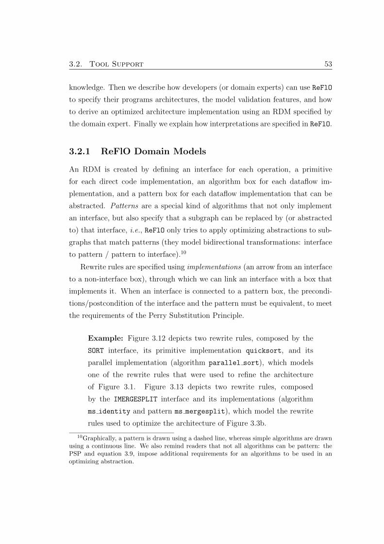
3.2. Tool Support 53
knowledge. Then we describe how developers (or domain experts) can use ReFlO
to specify their programs architectures, the model validation features, and how
to derive an optimized architecture implementation using an RDM specified by
the domain expert. Finally we explain how interpretations are specified in ReFlO.
3.2.1 ReFlO Domain Models
An RDM is created by defining an interface for each operation, a primitive
for each direct code implementation, an algorithm box for each dataflow im-
plementation, and a pattern box for each dataflow implementation that can be
abstracted. Patterns are a special kind of algorithms that not only implement
an interface, but also specify that a subgraph can be replaced by (or abstracted
to) that interface, i.e., ReFlO only tries to apply optimizing abstractions to sub-
graphs that match patterns (they model bidirectional transformations: interface
to pattern / pattern to interface).10
Rewrite rules are specified using implementations (an arrow from an interface
to a non-interface box), through which we can link an interface with a box that
implements it. When an interface is connected to a pattern box, the precondi-
tions/postcondition of the interface and the pattern must be equivalent, to meet
the requirements of the Perry Substitution Principle.
Example: Figure 3.12 depicts two rewrite rules, composed by the
SORT interface, its primitive implementation quicksort, and its
parallel implementation (algorithm parallel sort), which models
one of the rewrite rules that were used to refine the architecture
of Figure 3.1. Figure 3.13 depicts two rewrite rules, composed
by the IMERGESPLIT interface and its implementations (algorithm
ms identity and pattern ms mergesplit), which model the rewrite
rules used to optimize the architecture of Figure 3.3b.
10Graphically, a pattern is drawn using a dashed line, whereas simple algorithms are drawnusing a continuous line. We also remind readers that not all algorithms can be pattern: thePSP and equation 3.9, impose additional requirements for an algorithms to be used in anoptimizing abstraction.

54 3. Encoding Domains: Refinement and Optimization
Figure 3.12: SORT interface, parallel sort algorithm, quicksort primitive, andtwo implementation links connecting the interface with their implementations,defining two rewrite rules.
Figure 3.13: IMERGESPLIT interface, ms identity algorithm, ms mergesplit
pattern, and two implementation links connecting the interface with the algo-rithm and pattern, defining two rewrite rules.
The rewrite rules are grouped in layers. Layers have the attribute active to
specify whether their implementations (rewrite rules) may be used when deriving
an architectures or not (i.e., easily allowing a group of rules to be disabled). Ad-
ditionally, layers have the attribute order that contains an integer value. When
deriving an architecture, we can also restrict the rewrite rules to be used to those
whose order is in a certain interval, limiting the set of rules that the ReFlO tries
to apply when deriving architectures, thus improving its performance.11
Rewrite rules must be documented so that others who inspect architecture
derivations can understand the steps that were used to derive it. Boxes, ports
11In some domains it is possible to order layers in such a way that initially we can onlyapply rewrite rules from the first layer, then we can only apply rules from a second layer, andso on. The order attribute allows us to define such an order.

3.2. Tool Support 55
and layers have the doc attribute, where domain experts can place a textual de-
scription of the model elements. ReFlO provides the ability to generate HTML
documentation, containing the figures of boxes, and their descriptions. This abil-
ity is essential to describe the transformations and elements of an RDM, thereby
providing a form of “documentation” that others could access and explore.
Besides the constraints mentioned in Section 3.1.1, ReFlO adds constraints
regarding names of boxes, ports and additional parameters, which must match
the regular expression [a− zA− Z0− 9 ]+. Additionally, a box can only be the
target of an implementation link.
Figure 3.14 depicts the UML class diagram of the metamodel for RDMs. The
constraints associated with this metamodel have been defined prior to this point.
name : Stringreplicated : Stringdoc : String
Element
parameters : String
Box
template : String
Interface
Algorithm
Implementation
Pattern
Connector
dataType : String
Port
Output
Input
1 source
1
target
*ports *
1source
outgoing
*1target
incoming
* elements
connectors *
Primitive
name : Stringactive : Booleanorder : Integerdoc : String
Layer
*elementsimplementations*
Figure 3.14: ReFlO Domain Models UML class diagram.
Figure 3.15 shows the user interface provided by ReFlO. We have a project
that groups files related to a domain, containing folders for RDMs, architectures,
interpretations, documentation, etc. When we have an RDM opened (as show
in Figure 3.15), we also have a pallete on the right with objects and links we
can drag to the RDM file to build it. On the bottom we can see a window that
allows us to set attributes of the selected object.

56 3. Encoding Domains: Refinement and Optimization
Folder for interpretations
Folder for architectures
Folder for RDMs
RDM opened in the main window
Main window
Layer
Objects we can drag to an RDM
RDM opened
Selected box
Attributes of the selected box
Links we can drag to an RDM
Folder for documentation
Figure 3.15: ReFlO user interface.
3.2.1.1 Additional Parameters
Boxes have the attribute parameters to hold a comma-separated list of names,
data types and values, which specify their additional parameters. Each element
of the list of parameters should have the format name : datatype (if the param-
eter’s value is undefined), or name : datatype = value (if we want to provide a
value). The $ sign is used to specify a value that is a parameter of the parent box
(e.g., x : T = $y, where y is an additional parameter of the parent box, means
that parameter x, of type T, has the same value as y). Additional parameters
keep the models simpler (as they are not graphically visible), allowing developers
to focus on the essential parts of the model.
Example: Consider the algorithm parallel sort, presented in Fig-
ure 3.12. It has an additional parameter, to define the attribute to
use as key when comparing the input tuples. It is specified by the
expression SortKey : Attribute. Its internal box SORT also has an
additional parameter for the same purpose, and which value is equal

3.2. Tool Support 57
to the value of its parent box (parallel sort). Thus, it is specified
by the expression SortKey : Attribute = $SortKey.
3.2.1.2 Templates
Templates provide a way to easily specify several different rewrite rules that have
a common “shape”, and differ only on the name of the boxes. In that case, the
name of a particular box present in a rewrite rule denotes a variable, and we
use the attribute template of the LHS of the rewrite rule to specify the possible
instantiations of the variables present in the rewrite rule. Templates provide an
elementary form of higher-order transformations [TJF+09] that reduces modeling
effort.
Example: Consider the boxes of Figure 3.16, where F2 = F−11 . We
have the specification of an optimization. Whenever we have a box
F1 followed by a box F2 (algorithm IdF1F2), the second one can be
removed (algorithm IdF1). A similar optimization can be defined for
any pair of boxes (x1, x2), such that x2 = x−11 .
Figure 3.16: Two implementations of the same interface that specify an opti-mization.
Templates specify all such optimizations with the same set of boxes.
Assuming that G2 = G−11 and H2 = H−11 , we can express the three
different optimizations (that remove box F2, G2, or H2) creating the

58 3. Encoding Domains: Refinement and Optimization
Figure 3.17: Expressing optimizations using templates. The boxes optid, idx1,idx1x2, x1, and x2 are “variables” that can assume different values.
models depicted in Figure 3.17, and setting the attribute template of
box optid with the value
(optid , idx1, idx1x2, x1, x2) :=
(OptIdF, IdF1, IdF1F2, F1, F2) |(OptIdG, IdG1, IdG1G2, G1, G2) |(OptIdH, IdH1, IdH1H2, H1, H2)
The left-hand side of := specifies that optid, idx1, idx1x2, x1, and
x2 are “variables” (not the box names), which can be instantiated
with the values specified on the right-hand side. The symbol | sep-
arates the possible instantiations. For example, when instantiating
the variables with OptIdF, IdF1, IdF1F2, F1 and F2, we get the op-
timization of Figure 3.16.
3.2.1.3 Replicated Elements
Figure 3.12 showed a parallel algorithm for SORT, the parallel sort, where we
execute two instances of SORT in parallel. However, we are not limited to two,
and we could increase parallelism using more instances of SORT. Similarly, the
number of output ports of SPLIT boxes used in the algorithm, as well as the
input ports of SMERGE, may vary.

3.2. Tool Support 59
ReFlO allows to express this variability in models, using replicated elements.
Ports and boxes have an attribute that specifies their replication. This attribute
should be empty, in case the element is not replicated, or contain an upper
case letter, which is interpreted as a variable that specifies how many times the
element is replicated, and that we refer to as replication variable (this variable
is shown next to the name of the element, inside square brackets).12 Thus, box
B[N] means that there are N instances of box B (Bi, for i = {1...N}). Similarly for
ports.
Example: Using replicated elements, we can express the
parallel sort in a more flexible way, as depicted in Figure 3.18.
Output port O of SPLIT, interface SORT, and input port I of SMERGE
are replicated N times. Notice that we used the same value (N) in
all elements, meaning that they are replicated the same number of
times.
Figure 3.18: parallel sort algorithm modeled using replicated elements.
Example: We may have elements that can be replicated a different
number of times, as in the case of the interface IMERGESPLIT and its
implementations, msnm mergesplit and msnm splitmerge, depicted
in Figure 3.19. Here, the interface has N inputs and M outputs. Inside
the patterns we also have some elements replicated N times, and oth-
ers replicated M times. The scope of these variables is formed by all
connected boxes, which means that N and M used in the algorithms
are the same used in the interface they implement. This is impor-
tant in transformations, as we have to preserve these values, i.e., the
12These variables can be instantiated when generating code.

60 3. Encoding Domains: Refinement and Optimization
replication variables of the elements to remove during a transforma-
tion are used to determine the replication variables of the elements
to add. More on this in Section 3.2.4.
Figure 3.19: IMERGESPLITNM interface, and its implementationsmsnm mergesplit and msnm splitmerge, modeled using replicated elements.
ReFlO has specific rules for replicating connectors (i.e., connectors linking
replicated ports or ports of replicated boxes). Using the notation B.P to represent
port P of box B, given a connector from output port O of box B to input port I
of box C, the rules are:
• When O is replicated N times and B is not (which implies that either I or C
is also replicated N times), connectors link B.Oi to C.Ii or Ci.I (depending
on which is replicated), for i ∈ {1 . . . N}.
• When B is replicated N times and O is not (which implies that either I or C
is also replicated N times), connectors link Bi.O to C.Ii or Ci.I (depending
on which is replicated), for i ∈ {1 . . . N}.
• When B is replicated N times and O is replicated M times (which implies that
both C and I are also replicated), connectors link Bi.Oj to Cj.Ii, thereby
implementing a crossbar, for i ∈ {1 . . . N} and j ∈ {1 . . . M} (this also
implies that C is replicated M times, and I is replicated N times).
Example: According to these rules, the pattern msnm splitmerge
from Figure 3.19 results in the pattern depicted in Figure 3.20, when

3.2. Tool Support 61
N is equal to 2 and M is equal to 3. Notice the crossbar in the mid-
dle, resulting from a connector that was linking replicated ports of
replicated boxes.
Figure 3.20: msnm splitmerge pattern without replication.
3.2.2 Program Architectures
An architecture models a program that, with the help of an RDM, can be op-
timized to a specific need (such as a hardware platform). We use a slightly
different metamodel to express architectures. Figure 3.21 depicts the UML class
diagram of the metamodel for architectures.
name : Stringreplicated : Stringlabel : String
Element
parameters : String
Box
Primitive
Algorithm
Architecture
Connector
dataType : String
Port
Output
Input
*ports *
1source
outgoing
*1target
incoming
* elements connectors *
Interface
Figure 3.21: Architectures UML class diagram.
To model a program, we start with an architecture box specifying its inputs

62 3. Encoding Domains: Refinement and Optimization
and outputs, and a possible composition of interfaces that produces the desired
behavior. We may use additional parameters to model some of the inputs of the
program. As in RDMs, architectures may contain replicated elements.
Example: Several architectures were previously shown (e.g., Fig-
ure 3.1, 3.3a, and 3.5).
3.2.3 Model Validation
ReFlO provides the ability to validate RDMs and architectures, checking if they
meet the metamodel constraints. It checks whether the boxes have valid names,
whether the ports and parameters are unique and have valid names, and whether
inherited parameters are valid. Additionally, it also checks whether the ports
have the needed connectors, whether the connectors belong to the right box, and
whether the replication variables of connected ports and boxes are compatible.
For RDMs, it also checks whether primitives and algorithms implement an
interface, and whether they have the same ports and additional parameters of
the interface they implement.
3.2.4 Model Transformations
ReFlO provides transformations to allow us to map architectures to more efficient
ones, optimized for particular scenarios. When creating an architecture, we
associate an RDM to it. The RDM specifies the transformations that we are
able to apply to the architecture. At any time during the mapping process, we
have the freedom to add new transformations to the RDM, which we want to
apply, but that are not available yet.
The transformations that can be applied to boxes inside an architecture are
described below:
Refine replaces an user selected interface with one of its implementations.
ReFlO examines the rewrite rules in order to determine which ones meet

3.2. Tool Support 63
the constraints described in Section 3.1.4. Then, a list of valid implemen-
tations is shown to the user, for him to choose one (if only one option is
available, it is automatically chosen). If either the interface or its ports are
replicated, that information is preserved (i.e., the replication variables of
the interface are used to define the replication variable of the implementa-
tion). If the implementation has replication variables that are not present
in the interface being refined, the user is asked to provide a value for the
variable.13
Example: Using the rewrite rule presented in Figure 3.18 to
refine the architecture of Figure 3.1, the user is asked to provide
a value for replication variable N, and after providing the value
Y, the architecture of Figure 3.22 is obtained.
Figure 3.22: Architecture ProjectSort, after refining SORT with a parallel im-plementation that use replication.
Flatten removes the modular boundaries of the selected algorithm. If the al-
gorithm to be flattened was replicated, this information is pushed down to
its internal boxes.14
Find Optimization locates all possible matches for the patterns in the RDM
that exist inside a user selected algorithm or architecture. The interfaces
that are part of matches are identified setting their attribute label, which
is shown after their name.
13We could also keep the value used in the RDM. However, in some cases we want to usedifferent values when refining different instances of an interfaces (with the same algorithm).
14We do not allow the flattening of replicated algorithms that contain replicated boxes, asthis would require multidimensional replication.
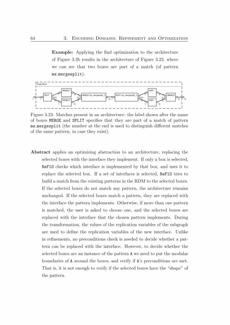
64 3. Encoding Domains: Refinement and Optimization
Example: Applying the find optimization to the architecture
of Figure 3.3b results in the architecture of Figure 3.23, where
we can see that two boxes are part of a match (of pattern
ms mergesplit).
Figure 3.23: Matches present in an architecture: the label shown after the nameof boxes MERGE and SPLIT specifies that they are part of a match of patternms mergesplit (the number at the end is used to distinguish different matchesof the same pattern, in case they exist).
Abstract applies an optimizing abstraction to an architecture, replacing the
selected boxes with the interface they implement. If only a box is selected,
ReFlO checks which interface is implemented by that box, and uses it to
replace the selected box. If a set of interfaces is selected, ReFlO tries to
build a match from the existing patterns in the RDM to the selected boxes.
If the selected boxes do not match any pattern, the architecture remains
unchanged. If the selected boxes match a pattern, they are replaced with
the interface the pattern implements. Otherwise, if more than one pattern
is matched, the user is asked to choose one, and the selected boxes are
replaced with the interface that the chosen pattern implements. During
the transformation, the values of the replication variables of the subgraph
are used to define the replication variables of the new interface. Unlike
in refinements, no preconditions check is needed to decide whether a pat-
tern can be replaced with the interface. However, to decide whether the
selected boxes are an instance of the pattern A we need to put the modular
boundaries of A around the boxes, and verify if A’s preconditions are met.
That is, it is not enough to verify if the selected boxes have the “shape” of
the pattern.

3.2. Tool Support 65
Optimize performs an optimizing abstraction, refinement and flattening as a
single step, replacing the selected set of boxes with an equivalent imple-
mentation.
Example: Applying the optimize transformation to the archi-
tecture of Figure 3.24a, to optimize the composition of boxes
MERGE− SPLIT, using the optimization from Figure 3.19, we get
the architecture of Figure 3.24b. Notice that during the transfor-
mation the replication variables of the original architecture are
preserved in the new architecture, i.e., the boxes being replaced
in the original architecture used X and Y instead of N and M (see
Figure 3.19), therefore the new architecture also uses X and Y
instead of N and M.
(a)
(b)
Figure 3.24: Optimizing a parallel version of the ProjectSort architecture.
Expand expands replicated boxes and ports of an architecture. For each repli-
cated box, a copy is created. For each replicated port, a copy is created,
and the suffixes 1 and 2 are added to the names of the original port and its
copy, respectively (as two port cannot have the same name). Connectors
are copied according to the rules previously defined.
Example: Figure 3.25 depicts the application of the expansion
transformation to the architecture of Figure 3.24b.

66 3. Encoding Domains: Refinement and Optimization
Figure 3.25: Expanding the parallel, replicated version of ProjectSort.
3.2.5 Interpretations
Each interpretation is written in Java. For a given interpretation, and a given
box, a Java class must be provided by the domain expert. Every interpreta-
tion is represented by a collection of classes—one per box—that is stored in a
unique Java package whose name identifies the interpretation. Thus if there are
n interpretations, there will be n Java packages provided by the domain expert.
compute() : voidgetAddParam(paramName : String) : StringgetBoxProperty(name : String) : ObjectgetParentProperty(name : String) : ObjectgetInputProperty(port : String, name : String) : ObjectgetOutputProperty(port : String, name : String) : ObjectsetBoxProperty(name : String, value : Object) : voidsetParentProperty(name : String, value : Object) : voidsetInputProperty(port : String, name : String, value : Object) : voidsetOutputProperty(port : String, name : String, value : Object) : voidaddError(errorMsg : String) : void
AbstractInterpretation
Figure 3.26: The AbstractInterpretation class.
Each class has the name of its box, and must extend abstract class
AbstractInterpretation provided by ReFlO (see Figure 3.26). Interpretations
grow in two directions: (i) new boxes can be added to the domain, which re-
quires new classes to be added to each package, and (ii) new interpretations can
be added, which requires new packages.
The behavior of an interpretation is specified in method compute. It com-
putes and stores properties that are associated with its box or ports. For each
box/port, properties are stored in a map that associates a value with a prop-
erty identifier. AbstractInterpretation provides get and set methods for
accessing and modifying properties.
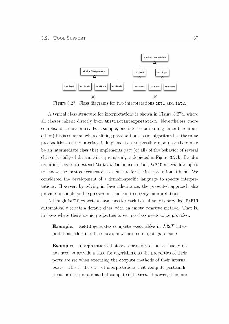
3.2. Tool Support 67
AbstractInterpretation
int1.BoxA int1.BoxB int2.BoxA int2.BoxB
(a)
AbstractInterpretation
int1.BoxA
int1.BoxB int2.BoxBint2.BoxA
int2.Super
(b)
Figure 3.27: Class diagrams for two interpretations int1 and int2.
A typical class structure for interpretations is shown in Figure 3.27a, where
all classes inherit directly from AbstractInterpretation. Nevertheless, more
complex structures arise. For example, one interpretation may inherit from an-
other (this is common when defining preconditions, as an algorithm has the same
preconditions of the interface it implements, and possibly more), or there may
be an intermediate class that implements part (or all) of the behavior of several
classes (usually of the same interpretation), as depicted in Figure 3.27b. Besides
requiring classes to extend AbstractInterpretation, ReFlO allows developers
to choose the most convenient class structure for the interpretation at hand. We
considered the development of a domain-specific language to specify interpre-
tations. However, by relying in Java inheritance, the presented approach also
provides a simple and expressive mechanism to specify interpretations.
Although ReFlO expects a Java class for each box, if none is provided, ReFlO
automatically selects a default class, with an empty compute method. That is,
in cases where there are no properties to set, no class needs to be provided.
Example: ReFlO generates complete executables in M2T inter-
pretations; thus interface boxes may have no mappings to code.
Example: Interpretations that set a property of ports usually do
not need to provide a class for algorithms, as the properties of their
ports are set when executing the compute methods of their internal
boxes. This is the case of interpretations that compute postcondi-
tions, or interpretations that compute data sizes. However, there are

68 3. Encoding Domains: Refinement and Optimization
cases where properties of an algorithm cannot be inferred from its
internal boxes. A prime example is the do nothing algorithm—it
has preconditions, but its internals suggest nothing. (In such cases,
a Java class is written for an algorithm to express its preconditions.)
ReFlO executes an interpretation in the following way: for each box in a graph,
its compute method is executed, with the execution order being determined
by the topological order of the boxes (in the case of hierarchical graphs, the
interpretation of an algorithm box is executed before the interpretations of its
internal boxes).15 After execution, a developer (or ReFlO tool) may select any
box and examine its properties.
Composition of Interpretations. Each interpretation computes certain
properties of a program P, and it may need properties that are also needed
by other interpretations, e.g., to estimate the execution cost of a box, we may
need an estimate of the volume of data output by a box. The same property
(volume of data) may be needed for other interpretations (e.g., preconditions).
Therefore, it is useful to separate the computation of each property, in order to
improve interpretation modularity and reusability.
ReFlO supports the composition of interpretations, where two or more in-
terpretations are executed in sequence, and an interpretation has access to the
properties computed by previously executed interpretations. For example, an
interpretation to compute data sizes (DS) can be composed with one that forms
cost estimates (ET ) to produce a compound interpretation (ET ◦ DS)(P) =
ET (P)◦DS(P). The same interpretation DS can be composed (reused) with any
other interpretation that also needs data sizes. PRE ◦POST is a typical exam-
ple where different interpretations are composed. In Section 4.2.4.3 we also show
how this ability to compose interpretations is useful when adding new rewrite
rules to an RDM.
15Backward interpretations reverse the order of execution, that is, a box is executed beforeits dependencies, and internal boxes are executed before their parent boxes.

Chapter 4
Refinement and Optimization
Case Studies
We applied the proposed methodology in different case studies from different
application domains, to illustrate how the methodology and tools can be used to
help developers deriving optimized program implementations in those domains,
and how we can make the derivation process understandable for non-experts
by exposing complex program architectures as a sequence of small incremental
transformations applied to an initial high-level program architecture.
In this chapter we present case studies from the relational databases and DLA
domains. First we describe simple examples, based on the equi-join relational
database operation, which is well-known for computer scientists, and therefore
can be easily appreciated by others. Then we describe more complex examples
from the DLA domain, where we show how we map the same initial architecture
(PIM) to architectures optimized for different hardware configurations (PSMs).
4.1 Modeling Database Operations
In this section we show how optimized programs from the relational databases
domain are derived. We start by presenting a detailed analysis of the derivation
of a Hash Join parallel implementation [GBS14], and its interpretations. Then
69

70 4. Refinement and Optimization Case Studies
we present a more complex variation of the Hash Join derivation.
4.1.1 Hash Joins in Gamma
Gamma was (and perhaps still is) the most sophisticated relational database
machine built in academia [DGS+90]. It was created in the late 1980s and
early 1990s without the aid of modern software architectural models. We focus
on Gamma’s join parallelization, which is typical of modern relational database
machines, and use ReFlO screenshots to incrementally illustrate Gamma’s deriva-
tions.
4.1.1.1 Derivation
A hash join is an implementation of a relational equi-join; it takes two streams
of tuples as input (A and B), and produces their equi-join A on B as output (AB).
Figure 4.1 is Gamma’s PIM. It just uses the HJOIN interface to specify the desired
behavior.
Figure 4.1: The PIM: Join.
Figure 4.2: bloomfilterhjoin algorithm.
The derivation starts by re-
fining the HJOIN interface with
its bloomfilterhjoin implemen-
tation, depicted in Figure 4.2.
The bloomfilterhjoin algorithm
makes use of Bloom filters [Blo70]
to reduce the number of tuples to
join. It uses two new boxes: BLOOM (to create the filter) and BFILTER (to apply
the filter). Here is how it works: the BLOOM box takes a stream of tuples A as
input and outputs exactly the same stream A along with a bitmap M. The BLOOM
box first clears M. Each tuple of A is read, its join key is hashed, the correspond-

4.1. Modeling Database Operations 71
ing bit (indicated by the hash) is set in M, and the A tuple is output. After all A
tuples are read, M is output. M is the Bloom filter.
The BFILTER box takes Bloom filter M and a stream of tuples A as input, and
eliminates tuples that cannot join with tuples used to build the Bloom filter.
The algorithm begins by reading M. Stream A is read one tuple at a time; the A
tuple’s join key is hashed, and the corresponding bit in M is checked. If the bit
is unset, the A tuple is discarded as there is no tuple to which it can be joined.
Otherwise the A tuple is output. A new A stream is the result.
Finally, output stream A of BLOOM and output stream A of BFILTER are joined.
Given the behaviors of the BLOOM, BFILTER, and HJOIN boxes, it is easy to prove
that bloomfilterhjoin does indeed produce A on B [BM11].
After applying the refinement transformation, we obtain the architecture de-
picted in Figure 4.3. The next step is to parallelize the BLOOM, BFILTER, and
HJOIN operations by refining each with their map-reduce implementations.
Figure 4.3: Join architecture, using Bloom filters.
Figure 4.4: parallelhjoin algorithm.
The parallelization of HJOIN is
textbook [BFG+95]: both input
streams A, B are hash-split on their
join keys using the same hash func-
tion. Each stream Ai is joined with
stream Bi (i ∈ {1, 2}), as we know
that Ai on Bj = ∅ for all i 6= j (equal
keys must hash to the same value).
By merging the joins of Ai on Bi (i ∈ {1, 2}), A on B is produced as output. This
parallel implementation of HJOIN is depicted in Figure 4.4.

72 4. Refinement and Optimization Case Studies
Figure 4.5: parallelbloom algorithm.
The BLOOM operation is paral-
lelized by hash-splitting its input
stream A into substreams A1, A2, cre-
ating a Bloom filter M1, M2 for each
substream, coalescing A1, A2 back
into A, and merging bit maps M1, Mn
into a single map M. This parallel
implementation of BLOOM is depicted in Figure 4.5.
Figure 4.6: parallelbfilter algorithm.
The BFILTER operation is par-
allelized by hash-splitting its in-
put stream A into substreams A1, A2.
Map M is decomposed into submaps
M1, M2 and substream Ai is filtered
by Mi. The reduced substreams
A1, A2 output by BFILTER are coa-
lesced into stream A. This parallel implementation of BFILTER is depicted in
Figure 4.6.
After applying the transformation, we obtain the architecture depicted in
Figure 4.7. We reached the point where refinement is insufficient to obtain the
Gamma’s optimized implementation.
Figure 4.7: Parallelization of Join architecture.
The architecture depicted in Figure 4.7 (after flattened) exposes three se-
rialization bottlenecks, which degrade performance. Consider the MERGE of
substreams A1, A2 (produced by BLOOM) into A, followed by a HSPLIT to re-
construct A1, A2. There is no need to materialize A: the MERGE − HSPLIT
composition can also be implemented by the identity map: Ai → Ai.

4.1. Modeling Database Operations 73
Figure 4.8: Optimization rewrite rules for MERGE−HSPLIT.
The same applies for the
MERGE − HSPLIT composi-
tion for collapsing and recon-
structing substreams pro-
duced by BFILTER. The
transformations required to
remove these bottlenecks are
encoded in the rewrite rules
depicted in Figure 4.8. The
removal of MERGE − HSPLIT
compositions eliminates two
serialization bottlenecks.
Figure 4.9: Optimization rewrite rules for MMERGE−MSPLIT.
The third bottleneck
combines maps M1, M2 into M,
and then decomposes M back
into M1, M2. The MMERGE −MSPLIT composition can also
be implemented by an iden-
tity map: Mi → Mi. This
optimization removes the
MMERGE − MSPLIT boxes and
reroutes the streams appropriately. It is encoded by the rewrite rules depicted
in Figure 4.9.
Figure 4.10: Join architecture’s bottlenecks.
Using the Find Optimization tool available in ReFlO, the bottlenecks are
identified, as depicted in Figure 4.10. These bottlenecks can be removed using
optimizations, which replace the inefficient compositions of operations by iden-
tities. Doing so, we obtain the optimized architecture depicted in Figure 4.11.
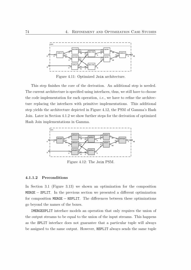
74 4. Refinement and Optimization Case Studies
Figure 4.11: Optimized Join architecture.
This step finishes the core of the derivation. An additional step is needed.
The current architecture is specified using interfaces, thus, we still have to choose
the code implementation for each operation, i.e., we have to refine the architec-
ture replacing the interfaces with primitive implementations. This additional
step yields the architecture depicted in Figure 4.12, the PSM of Gamma’s Hash
Join. Later in Section 4.1.2 we show further steps for the derivation of optimized
Hash Join implementations in Gamma.
Figure 4.12: The Join PSM.
4.1.1.2 Preconditions
In Section 3.1 (Figure 3.13) we shown an optimization for the composition
MERGE − SPLIT. In the previous section we presented a different optimization
for composition MERGE − HSPLIT. The differences between these optimizations
go beyond the names of the boxes.
IMERGESPLIT interface models an operation that only requires the union of
the output streams to be equal to the union of the input streams. This happens
as the SPLIT interface does not guarantee that a particular tuple will always
be assigned to the same output. However, HSPLIT always sends the same tuple

4.1. Modeling Database Operations 75
to the same output, and it has postconditions regarding the hash values of the
tuples of each output, which specify (i) a certain field was used to hash-split
the tuples, and (ii) that the outputs of port Ai, after being hashed, were as-
signed to substream of index i. The same postconditions are associated with
pattern mhs mergehsplit. Also note that pattern mhs mergehsplit needs an
additional parameter (SplitKey), which specifies the attribute to be used when
hash-splitting the tuples (and that is used to define the postconditions).
As required by the PSP, the postconditions of the dataflow graph to be
abstracted (pattern mhs mergehsplit) have to be equivalent to the postcon-
ditions of the interface it implements, thus, interface IMERGEHSPLIT also must
provide such postconditions. Through the use of the HSPLIT boxes, pattern
mhs hsplitmerge provides such postconditions.
IMERGEHSPLIT has one more implementation, mhs identity, that imple-
ments the interface using identities. The only way to guarantee that the outputs
of the identity implementation have the desired postconditions (properties), is to
require their inputs to already have them (as properties are not changed inter-
nally). Therefore, the mhs identity algorithm needs preconditions. This algo-
rithm can only be used if the input substreams are hash-split using the attribute
specified by SplitKey (that is also an additional parameter of mhs identity),
and if input Ai contains the substream i produced by the hash-split operation.
Specifying Postconditions. To specify postconditions, we use the following
properties: HSAttr is used to store the attribute used to hash-split a stream, and
HSIndex is used to store the substream to which the tuples were assigned. For
each box, we need to specify how these properties are affected. For example, the
HSPLIT interface sets such properties. On the other hand, MERGE removes such
properties (sets them to empty values). Other boxes, such as BLOOM and BFILTER
preserve the properties of the inputs (i.e., whatever is the property of the input
stream, the same property is used to set the output stream). In Figure 4.13 we
show the code used to specify these postconditions for some of the boxes used,
which is part of the interpretation hash.

76 4. Refinement and Optimization Case Studies
public class HSPLIT extends AbstractInterpretation {public void compute() {String key = getAddParam("SplitKey");setOutputProperty("A1","HSAttr",key);setOutputProperty("A2","HSAttr",key);setOutputProperty("A1","HSIndex",1);setOutputProperty("A2","HSIndex",2);
}}
public class MERGE extends AbstractInterpretation {public void compute() {// by default, properties have the value null// thus, no code is needed
}}
public class BFILTER extends AbtractInterpretation {public void compute() {String attr=(String)getInputProperty("A","HSAttr");setOutputProperty("A","HSAttr",attr);Integer index=(Integer)getInputProperty("A","HSIndex");setOutputProperty("A","HSIndex",index);
}}
Figure 4.13: Java classes for interpretation hash, which specifies database oper-ations’ postconditions.
Specifying Preconditions. Now we have to specify the preconditions of
mhs identity. Here, we have to read the properties of the inputs, and check
if they have the desired values. That is, we need to check if the input streams
are already hash-split, and if the same attribute was used as key to hash-split
the streams. We do that comparing the value of the property HSAttr with the
value of the additional parameter SplitKey. Moreover, we also need to verify
if the tuples are associated with the correct substreams. That is, we need to
check if the property HSIndex of inputs A1 and A2 are set to 1 and 2, respec-
tively. If these conditions are not met, the method addError is called to signal
the failure in validating the preconditions (it also defines an appropriate error
message). In Figure 4.14 we show the code we use to specify the preconditions
for the mhs identity, which is part of the interpretation prehash.

4.1. Modeling Database Operations 77
public class mhs_identity extends AbstractInterpretation {public void compute() {
String key=getAddParam("SplitKey");String hsAttrA1= (String)getInputProperty("A1","HSAttr");String hsAttrA2= (String)getInputProperty("A2","HSAttr");Integer hsIndexA1= (Integer)getInputProperty("A1","HSIndex");Integer hsIndexA2= (Integer)getInputProperty("A2","HSIndex");if(!key.equals(hsAttrA1) || !key.equals(hsAttrA2)
|| hsIndexA1 != 1 || hsIndexA2 != 2) {addError("Input streams are not correctly split!");
}}
}
Figure 4.14: Java classes for interpretation prehash, which specifies databaseoperations’ preconditions.
4.1.1.3 Cost Estimates
During the process of deriving a PSM, it is useful for the developers to be able
to estimate values of quality attributes they are trying to improve. This is a
typical application for interpretations.
For databases, estimates for execution time are computed by adding the
execution cost of each interface or primitive present in a graph. The cost of an
interface or primitive is computed based on the size of the data being processed.
An interface cost is set to that of its most general primitive implementation. It is
useful to associate costs to interfaces (even though they do not have direct code
implementations), as this allows developers to estimate execution time costs at
early stages of the derivation process.
Size estimates are used to build a cost expression representing the cost of
executing interfaces and primitives. The size interpretation takes estimates
of input data sizes and computes estimates of output data sizes. We build a
string containing a cost symbolic expression, as during design time we do not
have concrete values for properties needed to compute costs. Thus, we associate
a variable (string) to those properties, and we use those strings to build the
symbolic expression representing the costs. phjoin is executed by reading each
tuple of stream A and storing it in a main-memory hash table (cHJoinAItem is
a constant that represents the cost of processing a tuple of stream A), and then

78 4. Refinement and Optimization Case Studies
each tuple of stream B is read and joined with tuples of A (cHJoinBItem is a
constant that represents the cost of processing a tuple of stream B). Thus, the
cost of phjoin is given by sizea∗cHJoinAItem+sizeb∗cHJoinBItem. As HJOIN
can always be implemented by phjoin, we can use the same cost expression for
HJOIN. Figure 4.15 shows the code used to generate a cost estimate for phjoin
primitive, which is part of the interpretation costs. The costs interpretation
is backward, as the costs of an algorithm are computed from the costs of its
internal boxes (i.e., we need to compute costs of internal boxes first). So the
costs are progressively sent to their parent boxes, until they reach the outermost
box, where the costs of all boxes are aggregated, providing a cost estimate for
the entire architecture. Figure 4.16 shows the code used by interpretations of
algorithm boxes, which simply add their costs to the aggregated costs stored on
their parent boxes.
public class phjoin extends AbstractInterpretation {public void compute() {String sizeA=(String)getInputProperty("A","Size");String sizeB=(String)getInputProperty("B","Size");String cost="("+sizeA+") * cHJoinAItem + ("
+sizeB+") * cHJoinBItem";setBoxProperty("Cost",cost);String parentCost=(String)getParentProperty("Cost");if(parentCost==null) parentCost=cost;else parentCost="("+parentCost+") + ("+cost+")";setParentProperty("Cost", parentCost);
}}
Figure 4.15: Java classe for interpretation costs, which specifies phjoin’s cost.
public class Algorithm extends AbstractInterpretation {public void compute() {String cost=(String) getBoxProperty("Cost");String parentCost=(String)getParentProperty("Cost");if(parentCost==null) parentCost=cost;else parentCost="("+parentCost+") + ("+cost+")";setParentProperty("Cost", parentCost);
}}
Figure 4.16: Java class that processes costs for algorithm boxes.

4.1. Modeling Database Operations 79
4.1.1.4 Code Generation
The final step of a derivation is the M2T transformation to generate the code
from the PSM.
ReFlO provides no hard-codedM2T capability; it uses a code interpretation
instead. Figure 4.18 depicts the code that is generated from the architecture of
Figure 4.17 (a PSM obtained refining the architecture from Figure 4.3 directly
with primitives).
Figure 4.17: Join architecture, when using bloomfilterhjoin refinement only.
import gammaSupport.*;import basicConnector.Connector;
public class Gamma extends ArrayConnectors implements GammaConstants {public Join(Connector inA, Connector inB, int joinkey1, int joinkey2,
Connector outAB) throws Exception {Connector c1 = outAB;Connector c2 = inA;Connector c3 = inB;Connector c4 = new Connector("c4");Connector c5 = new Connector("c5");Connector c6 = new Connector("c6");int pkey1= joinkey1;int pkey2= joinkey2;new Bloom(pkey1, c2, c5, c4);new BFilter(pkey2, c3, c6, c4);new HJoin(c5, c6, pkey1, pkey2, c1);
}}
Figure 4.18: Code generated for an implementation of Gamma.
We use a simple framework, where primitive boxes are implemented by a
Java class, which provides a constructor that receives as parameters the input
and output connectors, and the additional parameters. Those classes extend
interface Runnable, and the behavior of the boxes is specified by method run.
Code generation is done by first using interpretations that associate a unique
identifier to each connector, which is then used to define the variables that will

80 4. Refinement and Optimization Case Studies
store the connector in the code being generated. Then, each box generates a line
of code that calls its constructor with the appropriate connector’s variables as
parameters (the identifiers previously computed provide this information), and
sends the code to its parent box (see Figure 4.19).
public class HJOIN extends AbstractInterpretation {public void compute() {String keyA=getAddParam("JoinKeyA");String keyB=getAddParam("JoinKeyB");Integer inA=(Integer)getInputProperty("A", "VarId");Integer inB=(Integer)getInputProperty("B", "VarId");Integer outAB=(Integer)getOutputProperty("AB","VarId");String pCode=(String)getParentProperty("Code");if(pCode==null) pCode="";pCode="\t\tnew HJoin(c" + inA + ", c" + inB + ", p" +
keyA + ", p" + keyB + ", c" + outAB + ");\n" + pCode;setParentProperty("Code", pCode);
}}
Figure 4.19: Interpretation that generates code for HJOIN box.
Similarly to cost estimates, this is a backward interpretation, and the ar-
chitecture box will eventually gather those calls to the constructors. As a final
step, the interpretation of the architecture box is executed, and adds the variable
declarations, and the class declaration.
4.1.2 Cascading Hash Joins in Gamma
In the previous section we showed how to derive an optimized implementation
for a single Hash Join operation. However, Figure 4.12 is not the last word on
Gamma’s implementation of Hash Joins. We now show how we can go further,
and derive an optimized implementation for cascading joins, where the output
of one join becomes the input of another. Moreover, in this derivation we make
use of replication, to produce an implementation that offers a flexible level of
parallelization. The initial PIM is represented in the architecture of Figure 4.20.
As for the previous derivation, we start by refining HJOIN interfaces with its
bloomfilterhjoin implementation. The next step is again to parallelize the
interfaces present in the architecture (BLOOM, BFILTER and HJOIN). This step is,

4.1. Modeling Database Operations 81
Figure 4.20: The PIM: CascadeJoin.
Figure 4.21: Parallel implementation of database operations using replication.
however, slightly different from the previous derivation, as we are going to use
replication to define the parallel algorithms. Figure 4.21 shows the new parallel
algorithms.
After using these algorithms to refine the architecture, and flattening it, we
are again at the point where we need to apply optimizations to remove the
serialization bottlenecks. Like in the parallel algorithm implementations, we
have to review the optimizations, to take into account replication. Figure 4.22
shows the new rewrite rules that specify replicated variant of the optimizations
needed.

82 4. Refinement and Optimization Case Studies
Figure 4.22: Optimization rewrite rules using replication.
This allow us to obtain the architecture depicted in Figure 4.23, which is
essentially a composition of two instances of the architecture presented in Fig-
ure 4.11 (also using replication).
Figure 4.23: CascadeJoin after refining and optimizing each of the initial HJOINinterface.
This architecture further shows the importance of deriving the architectures,
instead of just using a pre-built optimized implementation for the operations
present in the initial PIM (in this case, HJOIN operations). The use of the op-
timized implementations for HJOIN would have resulted in an implementation
equivalent to the one depicted in Figure 4.23. However, when we compose two
(or more) instances of HJOIN, new opportunities for optimization arise. In this
case, we have a new serialization bottleneck, formed by a composition of boxes
MERGE (that merges the output streams of the first group of HJOINs) and HSPLIT
(that hash-splits the stream again). Unlike the bottlenecks involving MERGE and

4.1. Modeling Database Operations 83
HSPLIT previously described, cascading joins use different keys to hash the tu-
ples, so the partitioning of the stream before the merge operation is different from
the partitioning after the hash-split operation. Moreover, the number of inputs
of merge operation may be different from the number of outputs of hash-split
operation (note that two different replication variables are used in the architec-
ture of Figure 4.23), which does not match the pattern mhs mergehsplit (see
Figure 4.22).
Figure 4.24: Additional optimization’s rewrite rules.
Therefore, we need
new rewrite rules, to de-
fine how this bottleneck
can be abstracted and im-
plemented in a more effi-
cient way. We define in-
terface IMERGEHSPLITNM,
which models an opera-
tion that merges N input
substreams, and hash-splits the result in M output substreams, according to a
given split key attribute. There are two ways of implementing this interface. We
can merge the input substreams, and then hash-split the resulting stream, using
the algorithm mhsnm mergehsplit depicted in Figure 4.24. The dataflow graph
used to define this implementation matches the dataflow subgraph that repre-
sents the bottleneck we want to remove. An alternative implementation swaps
the order in which operations MERGE and HSPLIT are applied, i.e., each input
substream is hash-split into M substreams by one of the N instances of HSPLIT,
and the resulting substreams are sent to each of the M instances of MERGE. The
substreams with the same hash values are then merged. This behavior is imple-
mented by algorithm mhsnm hsplitmerge, depicted in Figure 4.24.
After applying this optimization, we obtain the architecture from Figure 4.25.
This derivation would be concluded replacing the interfaces with primitive im-
plementations.1
1For simplification, we will omit this step in this and future derivations.

84 4. Refinement and Optimization Case Studies
Figure 4.25: Optimized CascadeJoin architecture.
Recap. In this section we showed how we used ReFlO to explain the design
of Gamma’s Hash Join implementations. This was the first example of a non-
trivial derivation obtained with the help of ReFlO, which allow us to obtain the
Java code for the optimized parallel hash join implementation. This work has
also been used to conduct controlled experiments [FBR12, BGMS13] to evaluate
whether a derivational approach for software development, as proposed by DxT,
has benefits regarding program comprehension and easy of modification. More
on this in Chapter 7.
4.2 Modeling Dense Linear Algebra
In this section we illustrate how DxT and ReFlO can be used to derive optimized
programs in the DLA domain. We start by showing the derivation of unblocked
implementations from high-level specifications of program loop bodies (as they
contain the components that we need to transform). We take two programs from
the domain (LU factorization and Cholesky factorization), and we start building
the RDM at the same time we produce the derivations. We also define the in-
terpretations, in particular pre- and postconditions. At some point, we will have
enough knowledge in the RDM to allow us to derive optimized implementations
for a given target hardware platform.
Later, we add support for other target platforms or inputs. We keep the
previous data, namely the RDM and the PIMs, and we incrementally enhance
the RDM to support the new platform. That is, we add new rewrite rules—new
algorithms, new interfaces, new primitives, etc.—, we add new interpretations,
and we complete the previous interpretations to support the new boxes. The
new rewrite rules typically define new implementations specialized for a certain

4.2. Modeling Dense Linear Algebra 85
platform (e.g., implementations specialized for distributed matrices). Precondi-
tions are used to limit the application of rewrite rules when a certain platform
is being targeted.
The rewrite rules we use are not proven correct, but, even though they have
not been systematized before, they are usually well-known to experts.
In the next section we show the PIMs for LU factorization and Cholesky
factorization. We then show how different implementations (unblocked, blocked,
and distributed memory) are obtained from the PIMs, by incrementally enhanc-
ing the RDM (see Figure 4.26 for the structure of this section).
PIM(Section 4.2.1)
Unblocked(Section 4.2.2)
Blocked(Section 4.2.3)
Dist. Memory(Section 4.2.4)
Figure 4.26: DLA derivations presented.
4.2.1 The PIMs
We use the algorithms presented in Section 2.3.1 (Figure 2.6 and Figure 2.7)
to define our initial architectures (PIMs). The most important part of these
algorithms is their loop body, and it is this part that has to be transformed to
adapt the algorithm for different situations. Therefore, the architectures we use
express the loop bodies of the algorithms only.
4.2.1.1 LU Factorization
Figure 4.27: The PIM: LULoopBody.

86 4. Refinement and Optimization Case Studies
Figure 4.27 depicts the architecture LULoopBody, the initial architecture for
LU factorization (its PIM). The loop body is composed of the following sequence
of operations:
• LU : A11 = LU(A11)
• TRS : A21 = A21 TriU(A−111 )
• TRS : A12 = TriL(A−111 ) A12
• MULT : A22 = A22 - A21 A12
The LU interface specifies an LU factorization. The TRS interface specifies
an inverse-matrix product B = coeff · op(A−1) · B or B = coeff · B · op(A−1),
depending on the value of its additional parameter side. trans, tri, diag,
and coeff are other additional parameters of TRS. trans specifies whether the
matrix is transposed or not (op(A) = A or op(A) = AT). A is assumed to be
a triangular matrix, and tri specifies whether it is lower or upper triangular.
Further, diag specifies whether the matrix is unit triangular or not. In the case
of the first TRS operation listed above, for example, the additional parameters
side, tri, trans, diag and coeff have values RIGHT, UPPER, NORMAL, NONUNIT
and 1, respectively.
The MULT interface specifies a matrix product and sum C = alpha · op(A) ·op(B) + beta · C. Again, op specifies whether matrices shall be transposed or
not, according to additional parameters transA and transB. alpha and beta
are also additional parameters of MULT. In the case of the MULT operation listed
above the additional parameters transA, transB, alpha and beta have values
NORMAL, NORMAL, −1 and 1, respectively.
4.2.1.2 Cholesky Factorization
Figure 4.28 depicts the architecture CholLoopBody, the initial architecture for
Cholesky factorization (its PIM). The loop body is composed of the following
sequence of operations:

4.2. Modeling Dense Linear Algebra 87
Figure 4.28: The PIM: CholLoopBody.
• CHOL : A11 = Chol(A11)
• TRS : A21 = A21 TriL(A−T11 )
• SYRANK : A22 = A22 - A21 AT21
The CHOL interface specifies Cholesky factorization. The TRS interface was
already described. The SYRANK interface specifies a symmetric rank update B =
alpha ·A ·AT+beta ·B or B = alpha ·AT ·A+beta ·B, depending on the value of its
additional parameter trans. tri, alpha and beta are also additional parameters
of SYRANK. tri specifies whether the lower or the upper triangular part of the
matrix C should be used (that is supposed to be symmetric). In the case of the
SYRANK operation listed above the additional parameters tri, trans, alpha and
beta have values LOWER, NORMAL, −1 and 1.
4.2.2 Unblocked Implementations
We start by presenting the derivation of unblocked implementations. In this case,
input A11 is a scalar (a matrix of size 1 × 1), inputs A21 and A12 are vectors
(matrices of size n×1 and 1×n, respectively), and A22 is a square matrix of size
n× n. The derivation of the optimized implementation uses this information to
choose specialized implementations for inputs of the given sizes [vdGQO08].
4.2.2.1 Unblocked Implementation of LU Factorization
The first step in the derivation is to optimize LU interface (see Figure 4.27) for
inputs of size 1 × 1. In this situation, LU operation can be implemented by the
identity, which allows us to obtain the architecture depicted in Figure 4.29.
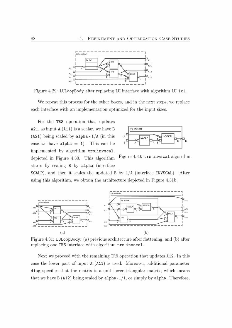
88 4. Refinement and Optimization Case Studies
Figure 4.29: LULoopBody after replacing LU interface with algorithm LU 1x1.
We repeat this process for the other boxes, and in the next steps, we replace
each interface with an implementation optimized for the input sizes.
Figure 4.30: trs invscal algorithm.
For the TRS operation that updates
A21, as input A (A11) is a scalar, we have B
(A21) being scaled by alpha · 1/A (in this
case we have alpha = 1). This can be
implemented by algorithm trs invscal,
depicted in Figure 4.30. This algorithm
starts by scaling B by alpha (interface
SCALP), and then it scales the updated B by 1/A (interface INVSCAL). After
using this algorithm, we obtain the architecture depicted in Figure 4.31b.
(a) (b)
Figure 4.31: LULoopBody: (a) previous architecture after flattening, and (b) afterreplacing one TRS interface with algorithm trs invscal.
Next we proceed with the remaining TRS operation that updates A12. In this
case the lower part of input A (A11) is used. Moreover, additional parameter
diag specifies that the matrix is a unit lower triangular matrix, which means
that we have B (A12) being scaled by alpha ·1/1, or simply by alpha. Therefore,

4.2. Modeling Dense Linear Algebra 89
TRS can be implemented by algorithm trs scal, which uses SCALP interface to
scale input B. This allows us to obtain the architecture depicted in Figure 4.32b.
(a) (b)
Figure 4.32: LULoopBody: (a) previous architecture after flattening, and (b) afterreplacing the remaining TRS interface with algorithm trs scal.
Figure 4.33: mult ger algorithm.
Finally we have the MULT interface. In-
puts A and B are vectors, and C is a matrix,
therefore, we use interface GER to perform the
multiplication. The algorithm to be used is
depicted in Figure 4.33. As MULT performs
the operation alpha · A · B + beta · C, and
GER, by definition, just performs the opera-
tion alpha · A · B + C, we also need to scale matrix C (interface SCALP). After
applying this algorithm, we obtain the architecture depicted in Figure 4.34b.
As the additional parameter alpha used by all SCALP interfaces has the value
1, these interfaces can be implemented by the identity, resulting in the archi-
tecture depicted in Figure 4.35b. Figure 4.36 is the final architecture, and ex-
presses an optimized unblocked implementation of LULoopBody. The PSM would
be obtained replacing each interface present in the architecture with a primitive
implementation.
4.2.2.2 Unblocked Implementation of Cholesky Factorization
The derivation starts by optimizing CHOL interface (see Figure 4.28) for inputs of
size 1× 1. In this case, CHOL operation is given by the square root of the input

90 4. Refinement and Optimization Case Studies
(a)
(b)
Figure 4.34: LULoopBody: (a) previous architecture after flattening, and (b) afterreplacing one MULT interface with algorithm mult ger.
(a)
(b)
Figure 4.35: LULoopBody: (a) previous architecture after flattening, and (b) afterreplacing SCALP interfaces with algorithm scalp id.

4.2. Modeling Dense Linear Algebra 91
Figure 4.36: Optimized LULoopBody architecture.
Figure 4.37: CholLoopBody after replacing Chol interface with algorithmchol 1x1.
value, as specified by algorithm chol 1x1. Applying this transformation allows
us to obtain the architecture depicted in Figure 4.37.
We proceed with the TRS operation. Input A (A11) is a scalar, therefore B
(A21) is scaled by alpha · 1/A, with alpha = 1. This allow us to use algorithm
trs invscal (previously depicted in Figure 4.30) to implement TRS. After using
this algorithm, we obtain the architecture depicted in Figure 4.38b.
Figure 4.39: syrank syr algorithm.
We then have the SYRANK operation.
Input A is a vector, and input B is a matrix,
therefore, we use interface SYR to perform
the operation. The algorithm to be used is
depicted in Figure 4.39. As for mult ger
(Figure 4.33), we also need interface SCALP
to scale matrix B by alpha. After applying this algorithm, we obtain the archi-
tecture depicted in Figure 4.40b.
As the additional parameter alpha used by all SCALP interfaces has the value
1, these interfaces can be implemented by the identity, resulting in the architec-
ture depicted in Figure 4.41b. Figure 4.42 is the final optimized architecture.
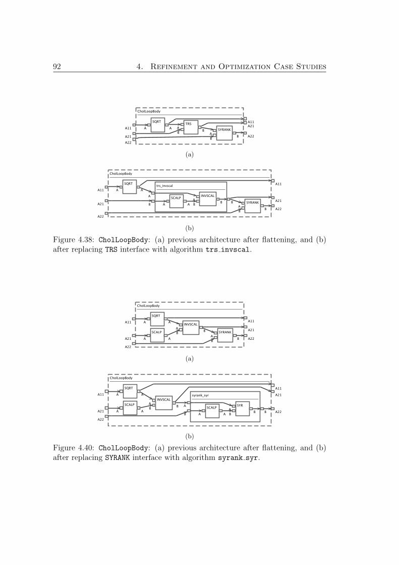
92 4. Refinement and Optimization Case Studies
(a)
(b)
Figure 4.38: CholLoopBody: (a) previous architecture after flattening, and (b)after replacing TRS interface with algorithm trs invscal.
(a)
(b)
Figure 4.40: CholLoopBody: (a) previous architecture after flattening, and (b)after replacing SYRANK interface with algorithm syrank syr.

4.2. Modeling Dense Linear Algebra 93
(a)
(b)
Figure 4.41: CholLoopBody: (a) previous architecture after flattening, and (b)after replacing SCALP interfaces with algorithm scalp id.
Figure 4.42: Optimized CholLoopBody architecture.
4.2.2.3 Preconditions
The derivation of the unblocked implementation of LULoopBody was obtained
by refining the architecture with interface implementations specialized for the
specified input sizes. Consider the rewrite rule (LU, lu 1x1) (Figure 4.43), which
provides an implementation specialized for the case where input matrix A of
LU has size 1x1. In this case, LU operation is implemented by identity (no
computation is needed at all). As we saw before, other interfaces have similar
implementations, optimized for different input sizes.
The specialized implementations are specified by associating preconditions
to rewrite rules, which check properties about the size of inputs. Moreover,
postconditions are used to specify how operations affect data sizes. We now

94 4. Refinement and Optimization Case Studies
Figure 4.43: (LU, lu 1x1) rewrite rule.
describe how the pre- and postconditions needed for the derivation of unblocked
implementations are specified.2
Specifying Postconditions. To specify the postconditions we use the follow-
ing properties: SizeM is used to store the number of rows of a matrix, and SizeN
is used to store the number of columns of a matrix. Each box uses these prop-
erties to specify the size of its outputs. In DLA domain, output size is usually
obtained copying the size of one of its inputs. In Figure 4.44 we show the code
we use to specify the postconditions for some of the boxes used, which is part
of interpretation sizes. We define class Identity11, which specifies how size is
propagated by interfaces with an input and an output named A, for which the
input size is equal to the output size. Interpretations for boxes such as LU or
SCALP can be defined simply extending this class. Similar Java classes are used
to define the sizes interpretation for other boxes.
Specifying Preconditions. Preconditions for DLA operations are specified
by checking whether the properties of inputs have the desired values. We also
have some cases where the preconditions check the values of additional parame-
ters. Figure 4.45 shows some of the preconditions used. Class AScalar specifies
preconditions for checking whether input A is a scalar. It starts by reading the
properties containing the input size information, and then it checks whether both
sizes are equal to 1. If not, addError method is used to signal a failure validating
preconditions. The preconditions for algorithms such as lu 1x1 or trs invscal
are specified simply extending this class. As we mentioned before, other algo-
rithms have more preconditions, namely to require certain values for additional
2Later we show how these pre- and postconditions are extended when enriching the RDMto support additional hardware platforms.

4.2. Modeling Dense Linear Algebra 95
public class Identity11 extends AbstractInterpretation {public void compute() {
String sizeM = (String) getInputProperty("A", "SizeM");String sizeN = (String) getInputProperty("A", "SizeN");setOutputProperty("A", "SizeM", sizeM);setOutputProperty("A", "SizeN", sizeN);
}}
public class LU extends Identity11 {// Reuses compute definition from Identity11
}
public class SCALP extends Identity11 {// Reuses compute definition from Identity11
}
Figure 4.44: Java classes for interpretation sizes, which specifies DLA opera-tions’ postconditions.
parameters. It is the case of algorithm trs scal, for example, which requires
its additional parameter diag to have the value UNIT, to specify that the input
A should be treated as a unit triangular matrix. Class trs scal (Figure 4.45)
shows how this requirement is specified. In addition to call the compute method
from its superclass (AScalar) to verify whether input A is a scalar, it obtains the
value of additional parameter diag, and checks whether it has the value UNIT.
Similar Java classes are used to define the preconditions for other boxes.
4.2.3 Blocked Implementations
Most of current hardware architectures are much faster performing computations
(namely floating point operations) than fetching data from memory. Therefore,
to achieve high-performance in DLA operations, it is essential to make a wise use
of CPU caches to compensate the memory access bottleneck [vdGQO08]. This
is usually done through the use of blocked algorithms [vdGQO08], having blocks
of data—where the number of operations is of higher order than the number of
elements to fetch from memory (e.g., cubic vs. quadratic)—processed together,
which enables a more efficient use of memory by taking advantage of different
levels of CPU caches.
In the following we show how loop bodies for blocked variants of programs

96 4. Refinement and Optimization Case Studies
public class AScalar extends AbstractInterpretation {public void compute() {String sizeM = (String) getInputProperty("A", "SizeM");String sizeN = (String) getInputProperty("A", "SizeN");if(!"1".equals(sizeM) || !"1".equals(sizeN)) {
addError("Input matrix A is not 1x1!");}
}}
public class lu_1x1 extends AScalar {}
public class trs_invscal extends AScalar {}
public class trs_scal extends AScalar {public void compute() {super.compute();String unit = (String) getAddParam("diag");if(!"UNIT".equals(unit)) {
addError("Input matrix A is not unit triangular!");}
}}
Figure 4.45: Java classes for interpretation presizes, which specifies DLA op-erations’ preconditions.
are derived from their PIMs. For this version, input A11 is a square matrix of
size b × b (the block size), inputs A21 and A12 are matrices of size n × b and
b× n, and A22 is a square matrix of size n× n. We refine the PIMs to produce
implementations optimized for inputs with these characteristics.
4.2.3.1 Blocked Implementation of LU Factorization
We start the derivation by replacing LU interface with its general implementation,
specified by algorithm lu blocked. This algorithm simply uses LU B interface,
which specifies the LU factorization for matrices. This transformation results in
the architecture depicted in Figure 4.46.
Next we replace both TRS interfaces with algorithm trs trsm, which uses
TRSM interface to perform the TRS operation. These transformations result in
the architecture depicted in Figure 4.47b.
Finally, we replace the MULT interface with algorithm mult gemm, which uses

4.2. Modeling Dense Linear Algebra 97
Figure 4.46: LULoopBody after replacing LU interface with algorithm lu blocked.
(a) (b)
Figure 4.47: LULoopBody: (a) previous architecture after flattening, and (b) afterreplacing both TRS interfaces with algorithm trs trsm.
(a) (b)
Figure 4.48: LULoopBody: (a) previous architecture after flattening, and (b) afterreplacing MULT interface with algorithm mult gemm.

98 4. Refinement and Optimization Case Studies
GEMM interface to perform the MULT operation. After applying this transformation
we get the architecture depicted in Figure 4.48b. After flattening, we get the
LULoopBody architecture for blocked inputs, depicted in Figure 4.49.
Figure 4.49: Optimized LULoopBody architecture.
4.2.3.2 Blocked Implementation of Cholesky Factorization
We start the derivation by refining CHOL interface with its general implemen-
tation, specified by algorithm chol blocked. It uses CHOL B interface, which
specifies the Cholesky factorization for matrices, resulting in the architecture
depicted in Figure 4.50.
Figure 4.50: CholLoopBody after replacing CHOL interface with algorithmchol blocked.
We then refine TRS interface with algorithm trs trsm, which uses TRSM inter-
face to perform the TRS operation. This transformation results in the architecture
depicted in Figure 4.51b.
Finally, we refine the SYRANK interface with algorithm syrank syrk, which
uses SYRK interface to perform the operation. After applying this transformation
we get the architecture depicted in Figure 4.52b, and after flattening it, we get
the CholLoopBody architecture for blocked inputs, depicted in Figure 4.53.

4.2. Modeling Dense Linear Algebra 99
(a)
(b)
Figure 4.51: CholLoopBody: (a) previous architecture after flattening, and (b)after replacing both TRS interfaces with algorithm trs trsm.
(a)
(b)
Figure 4.52: LULoopBody: (a) previous architecture after flattening, and (b) afterreplacing MULT interface with algorithm syrank syrk.

100 4. Refinement and Optimization Case Studies
Figure 4.53: Final architecture: CholLoopBody after flattening syrank syrk al-gorithms.
4.2.4 Distributed Memory Implementations
We now show how we can derive distributed memory implementations for DLA
programs. We achieve this by adding new rewrite rules. We also add new
interpretations to support additional pre- and postconditions required to express
the knowledge needed to derive distributed memory implementations. For these
derivations, we assume that the inputs are distributed using a [MC, MR] distribution
(see Section 2.3.1.6), and that several instances of the program are running in
parallel, each one having a different part of the input (i.e., the program follows
the SPMD model). We choose implementations (algorithms or primitives) for
each operation prepared to deal with distributed inputs [PMH+13].
4.2.4.1 Distributed Memory Implementation of LU Factorization
The starting point for this derivation is again the PIM LULoopBody (see Fig-
ure 4.27), which represents the loop body of the program that is executed by
each parallel instance of it.
Figure 4.54: dist2loca lu algorithm.
We start the derivation
with LU operation. We refine
LULoopBody replacing LU inter-
face with its implementation for
distributed memory, algorithm
dist2local lu (Figure 4.54).
The algorithm implements the operation by first redistributing input A. That
is, interface STAR STAR represents a redistribution operation, which uses col-
lective communications to obtain the same matrix in a different distribution

4.2. Modeling Dense Linear Algebra 101
(in this case [∗, ∗], which gathers all values of the matrix in all processes).3
We then call the LU operation on this “new” matrix, and we redistribute the
result (interface MC MR) to get a matrix with a [MC, MR] distribution so that the
behavior of the original LU interface is preserved (it takes a [MC, MR] matrix,
and produces a [MC, MR] matrix). By applying this transformation, we obtain the
architecture from Figure 4.55. Notice that we have again the LU operation in the
architecture. However, the input of LU is now a [∗, ∗] distributed matrix, which
enables the use of other LU implementations (such as the blocked and unblocked
implementations previously described).
Figure 4.55: LULoopBody after replacing LU interface with algorithmdist2local lu.
Figure 4.56: dist2loca trs algorithm.
The architecture is then re-
fined by replacing the TRS inter-
face that processes input A21 with a
distributed memory implementation.
We use algorithm dist2local trs
(Figure 4.56). The algorithm uses
again STAR STAR to gather all values
from input A (initially using a [MC, MR]
distribution). This is a templatized algorithm, where redist box, which re-
distributes input matrix B (also initially using a [MC, MR] distribution), may be a
STAR MC, MC STAR, STAR MR, MR START, STAR VC, VC STAR, STAR VR, VR STAR, or
3We use a b (a, b ∈ {∗, MC, MR, VC, VR}) to denote the redistribution operation that takesa matrix using any distribution, and converts it to a matrix using redistribution [a, b]. Forexample, MC MR converts a matrix to a new one using a [MC, MR] distribution. By having a singleredistribution operation for any input distribution (instead of one for each pair of input andoutput distributions), we reduce the number of redistribution operations we need to model(one per output distribution), and also the number of rewrite rules we need.

102 4. Refinement and Optimization Case Studies
STAR STAR redistribution. The algorithm has preconditions: STAR ∗ redistribu-
tions can only be used when the side additional parameter has value LEFT, and
∗ STAR redistributions can only be used when side has value RIGHT. In this case,
side has value RIGHT, and we choose the variant dist2local trs r3, which uses
MC STAR redistribution. The redistributed matrices are then sent to TRS, and the
output is redistributed by MC MR back to a matrix using [MC, MR] distribution. This
transformation yields the architecture depicted in Figure 4.57b. As for the pre-
vious refinement, the transformation results in an architecture where the original
box is present, but the inputs now use different distributions.
(a)
(b)
Figure 4.57: LULoopBody: (a) previous architecture after flattening, and (b) afterreplacing one TRS interface with algorithm dist2local trs r3.
Next we refine the architecture replacing the other TRS interface with a similar
algorithm. This instance of TRS has the value LEFT for additional parameter
side, therefore we use a different variant of the algorithm, dist2local trs l2,
which uses STAR VR redistribution. The resulting architecture is depicted in
Figure 4.58b.
We now proceed with interface MULT. This operation can be implemented in
distributed memory environments by algorithm dist2local mult (Figure 4.59).
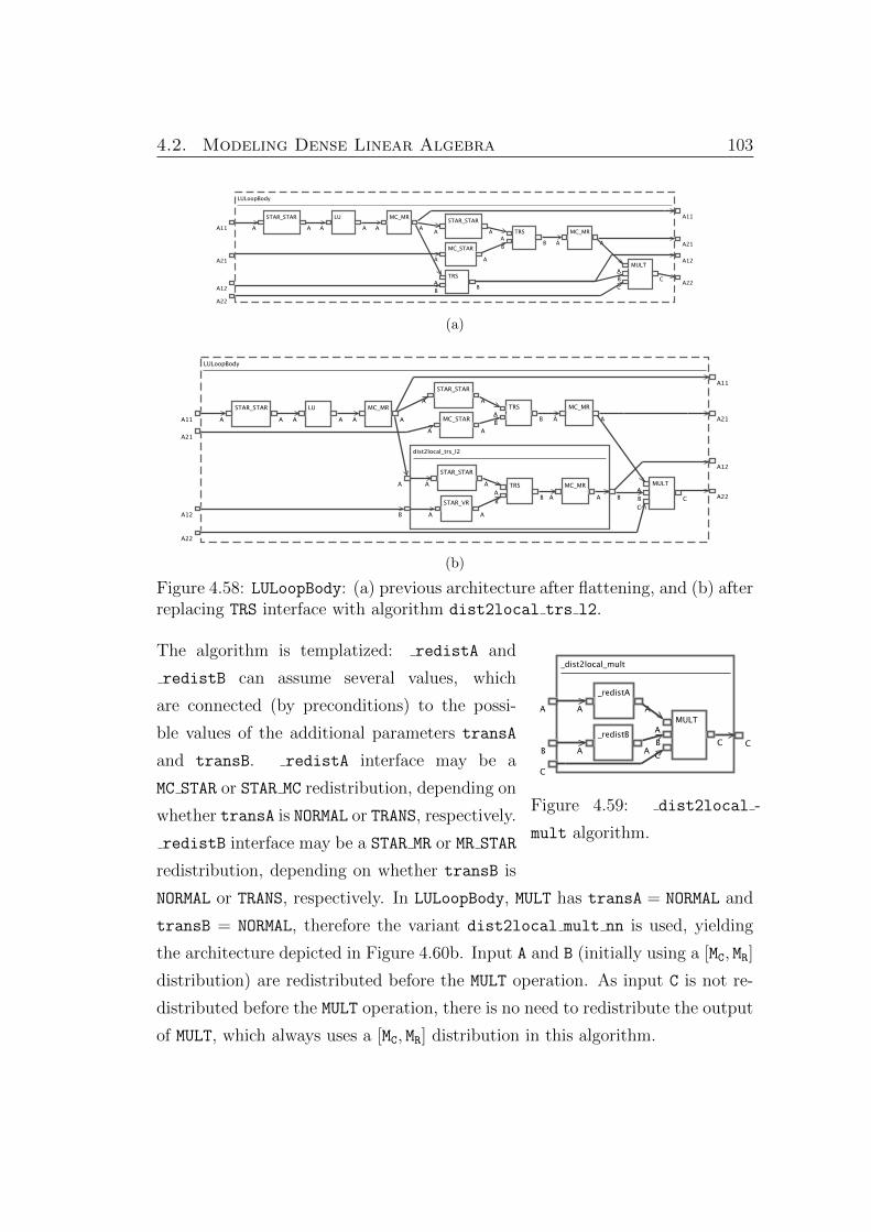
4.2. Modeling Dense Linear Algebra 103
(a)
(b)
Figure 4.58: LULoopBody: (a) previous architecture after flattening, and (b) afterreplacing TRS interface with algorithm dist2local trs l2.
Figure 4.59: dist2local -
mult algorithm.
The algorithm is templatized: redistA and
redistB can assume several values, which
are connected (by preconditions) to the possi-
ble values of the additional parameters transA
and transB. redistA interface may be a
MC STAR or STAR MC redistribution, depending on
whether transA is NORMAL or TRANS, respectively.
redistB interface may be a STAR MR or MR STAR
redistribution, depending on whether transB is
NORMAL or TRANS, respectively. In LULoopBody, MULT has transA = NORMAL and
transB = NORMAL, therefore the variant dist2local mult nn is used, yielding
the architecture depicted in Figure 4.60b. Input A and B (initially using a [MC, MR]
distribution) are redistributed before the MULT operation. As input C is not re-
distributed before the MULT operation, there is no need to redistribute the output
of MULT, which always uses a [MC, MR] distribution in this algorithm.
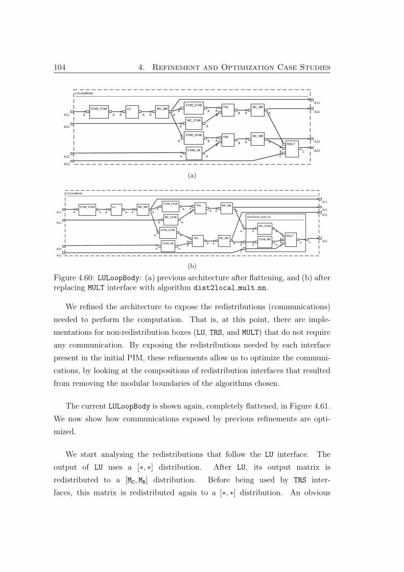
104 4. Refinement and Optimization Case Studies
(a)
(b)
Figure 4.60: LULoopBody: (a) previous architecture after flattening, and (b) afterreplacing MULT interface with algorithm dist2local mult nn.
We refined the architecture to expose the redistributions (communications)
needed to perform the computation. That is, at this point, there are imple-
mentations for non-redistribution boxes (LU, TRS, and MULT) that do not require
any communication. By exposing the redistributions needed by each interface
present in the initial PIM, these refinements allow us to optimize the communi-
cations, by looking at the compositions of redistribution interfaces that resulted
from removing the modular boundaries of the algorithms chosen.
The current LULoopBody is shown again, completely flattened, in Figure 4.61.
We now show how communications exposed by previous refinements are opti-
mized.
We start analysing the redistributions that follow the LU interface. The
output of LU uses a [∗, ∗] distribution. After LU, its output matrix is
redistributed to a [MC, MR] distribution. Before being used by TRS inter-
faces, this matrix is redistributed again to a [∗, ∗] distribution. An obvious

4.2. Modeling Dense Linear Algebra 105
Figure 4.61: LULoopBody flattened after refinements.
Figure 4.62: Optimization rewrite rules to remove un-
necessary STAR STAR redistribution.
optimization can be
applied, which con-
nects LU directly to the
TRS interfaces, remov-
ing the (expensive) re-
distribution operation
STAR STAR. This opti-
mization is expressed by
the rewrite rules from
Figure 4.62. The algo-
rithm boxes have a pre-
condition that requires the input to use a [∗, ∗] distribution. When this happens,
if we redistribute the input to any distribution, and then we redistribute back to
a [∗, ∗] distribution (pattern inv ss0), the STAR STAR interface can be removed
(algorithm inv ss1), as the output of STAR STAR is equal to the original input.
These rewrite rules are templatized, as the first redistribution ( redist) may be
any redistribution interface.
By applying the optimization expressed by these rewrite rules twice, we
remove both interior STAR STAR redistributions, obtaining the architecture de-
picted in Figure 4.63.
A similar optimization can be used to optimize the composition of re-
distributions that follows TRS interface that updates A21. In this case,
the output of TRS uses a [MC, ∗] distribution, and it is redistributed to

106 4. Refinement and Optimization Case Studies
Figure 4.63: LULoopBody after applying optimization to remove STAR STAR re-distributions.
Figure 4.64: Optimization rewrite rules to remove
unnecessary MC STAR redistribution.
[MC, MR], and then back to
[MC, ∗], before being used
by MULT. The rewrite rules
depicted in Figure 4.64
(similar to the one pre-
viously described in Fig-
ure 4.62) express this op-
timization. Its application
yields the architecture de-
picted in Figure 4.65.
Figure 4.65: LULoopBody after applying optimization to remove MC STAR redis-tributions.
Lastly, we analyse the interfaces that follow TRS interface updating matrix
A12. The output matrix uses a [∗, VR] distribution, and redistributions MC MR
and STAR MR are used to produce [MC, MR] and [∗, MR] distributions of the matrix.

4.2. Modeling Dense Linear Algebra 107
Figure 4.66: Optimization rewrite rules to swap
the order of redistributions.
However, the same behav-
ior can be obtained invert-
ing the order of the redis-
tributions, i.e., starting by
producing [∗, MC] matrix and
then using that matrix to pro-
duce a [MC, MR] distributed ma-
trix. This alternative compo-
sition of redistributions is also
more efficient, as we can ob-
tain a [MC, MR] distribution from
a [∗, MC] distribution simply discarding values (i.e., without communication
costs). This optimization is expressed by the rewrite rules from Figure 4.66,
where two templatized rewrite rules express the ability to swap the order of two
redistributions. In this case, redistA is MC MR, and redistB is STAR MR. After
applying this transformation, we obtain the optimized architecture depicted in
Figure 4.67.
Figure 4.67: Optimized LULoopBody architecture.
4.2.4.2 Distributed Memory Implementation of Cholesky
Factorization
To derive a distributed memory implementation for Cholesky factorization, we
start with the CholLoopBody PIM (see Figure 4.28), which represents the loop
body of the program that is executed by each parallel instance of it.

108 4. Refinement and Optimization Case Studies
Figure 4.68: dist2local chol algorithm.
The first step of the deriva-
tion is to refine the architec-
ture by replacing CHOL with an
algorithm for distributed mem-
ory inputs. We use the
dist2local chol algorithm, de-
picted in Figure 4.68. This algorithm is similar to dist2local lu. It implements
the operation by first redistributing input A (that initially uses a [MC, MR] distribu-
tion), i.e., interface STAR STAR is used to obtain a [∗, ∗] distribution of the input
matrix. Then CHOL operation is called on the redistributed matrix, and finally
we redistribute the result (interface MC MR) to get a matrix with a [MC, MR] distri-
bution. By applying this transformation, we obtain the architecture depicted in
Figure 4.69.
Figure 4.69: CholLoopBody after replacing CHOL interface with algorithmdist2local chol.
The next step is to refine the architecture by replacing TRS interface
with a distributed memory implementation. As for LULoopBody, we use
dist2local trs templatized implementation (see Figure 4.56). However, in
this case we choose algorithm dist2local trs r1, which uses VC STAR to re-
distribute input B. This transformation yields the architecture depicted in Fig-
ure 4.70b.
We proceed with interface SYRANK. For this interface, we use algo-
rithm dist2local syrank (Figure 4.71). This algorithm is templatized:
redistA and redistB can assume several values, which are connected (by
preconditions) to the possible values of the additional parameter trans.

4.2. Modeling Dense Linear Algebra 109
(a)
(b)
Figure 4.70: CholLoopBody: (a) previous architecture after flattening, and (b)after replacing TRS interface with algorithm dist2local trs r1.
Figure 4.71: dist2local syrank
algorithm.
In this case trans = NORMAL, there-
fore variant dist2local syrank n is used,
where redistA is MR STAR and redistB is
MC STAR. As input C is not redistributed be-
fore the TRRANK operation, there is no need
to redistribute the output of TRRANK, which
already uses [MC, MR] distribution. The trans-
formation yields the architecture depicted in
Figure 4.72b.
We reached again the point where we exposed the redistributions needed so
that each operation present in the initial PIM can be computed locally. The
current CholLoopBody is shown again, completely flattened, in Figure 4.73. We
proceed the derivation optimizing the compositions of redistributions introduced
in the previous steps.
We start analysing the redistributions that follow the CHOL interface. It
exposes the same inefficiency we saw after LU interface in LULoopBody (see Fig-
ure 4.61). The output of CHOL uses a [∗, ∗] distribution, and before the TRS
interface, this matrix is redistributed to a [MC, MR] distribution and then back to

110 4. Refinement and Optimization Case Studies
(a)
(b)
Figure 4.72: CholLoopBody: (a) previous architecture after flattening, and (b)after replacing SYRANK interface with algorithm dist2local syrank n.
Figure 4.73: CholLoopBody flattened after refinements.
Figure 4.74: CholLoopBody after applying optimization to remove STAR STAR
redistribution.
a [∗, ∗] distribution. Thus, we can remove redistribution operation STAR STAR,
reusing the optimization expressed by the rewrite rules presented in Figure 4.62,
which results in the architecture depicted in Figure 4.74.

4.2. Modeling Dense Linear Algebra 111
Figure 4.75: vcs mcs algorithm.
The next step in the derivation is to refine
the architecture expanding some of the redistri-
butions as a composition of redistributions, in
order to expose further optimization opportu-
nities. We replace MC STAR with its algorithm
vcs mcs (Figure 4.75), which starts by obtaining a [VC, ∗] distribution of the
matrix, and only then obtains the [MC, ∗] distribution.
Figure 4.76: vcs vrs mrs algorithm.
We also replace MR STAR with
its algorithm vcs vrs mrs (Fig-
ure 4.76), which starts by obtain-
ing a [VC, ∗] distribution of the
matrix, then obtains a [VR, ∗] dis-
tribution, and finally obtains the
[MR, ∗] distribution. These refinements result in the architecture depicted in Fig-
ure 4.77.
Figure 4.77: CholLoopBody after refinements that replaced MC STAR and MR STAR
redistributions.
The previous refinements exposed the redistribution VC STAR immediately
after the MC MR interface that redistributes the output of TRS. But the output
of TRS is already a matrix using a [VC, ∗] distribution, thus the VC STAR redis-
tributions can be removed. This is accomplished by applying an optimization
modeled by similar rewrite rules to the previously presented in Figure 4.62 and
Figure 4.64, which yields the architecture depicted in Figure 4.78.
There is one more redistribution optimization. From the output ma-
trix of TRS, we are obtaining directly a [MC, MR] distribution (MC MR) and a
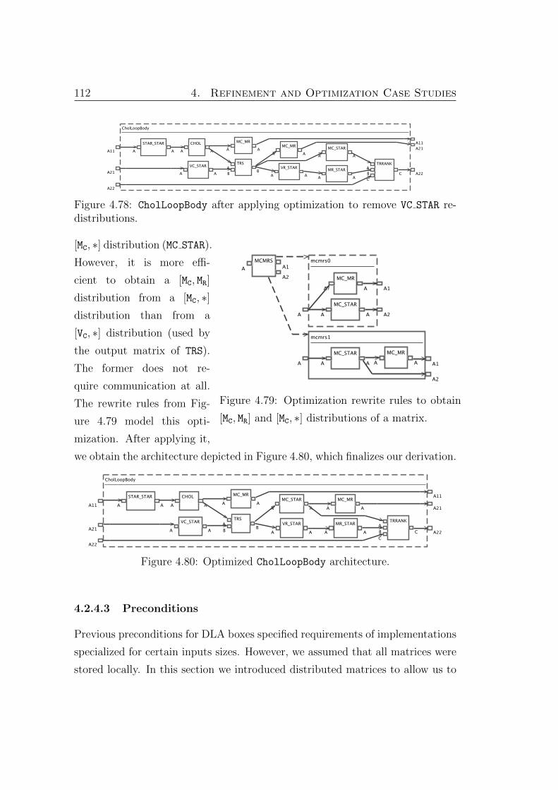
112 4. Refinement and Optimization Case Studies
Figure 4.78: CholLoopBody after applying optimization to remove VC STAR re-distributions.
Figure 4.79: Optimization rewrite rules to obtain
[MC, MR] and [MC, ∗] distributions of a matrix.
[MC, ∗] distribution (MC STAR).
However, it is more effi-
cient to obtain a [MC, MR]
distribution from a [MC, ∗]distribution than from a
[VC, ∗] distribution (used by
the output matrix of TRS).
The former does not re-
quire communication at all.
The rewrite rules from Fig-
ure 4.79 model this opti-
mization. After applying it,
we obtain the architecture depicted in Figure 4.80, which finalizes our derivation.
Figure 4.80: Optimized CholLoopBody architecture.
4.2.4.3 Preconditions
Previous preconditions for DLA boxes specified requirements of implementations
specialized for certain inputs sizes. However, we assumed that all matrices were
stored locally. In this section we introduced distributed matrices to allow us to

4.2. Modeling Dense Linear Algebra 113
derive implementations optimized for distributed memory hardware platforms.
This required the addition of new rewrite rules. It also requires a revision of pre-
and postconditions, which now should also take into account the distribution
of input matrices. Due to the ability to compose interpretations provided by
ReFlO, this can be achieved without modifying the previously defined pre- and
postconditions.
Specifying Postconditions. Besides the properties we already defined in
interpretation sizes (and that we have to specify for the new boxes added
to support distributed memory environments), we are going to define a new
property (postcondition), called Dist, that we use to store the distribution of
a matrix. This new postcondition is defined by a new interpretation, called
distributions. For each interface and primitive, we have to specify how the
distribution of its outputs is obtained. For redistribution interfaces, each one
determines a specific output’s distribution. For example, STAR STAR produces a
[∗, ∗] distributed matrix, and MC MR produces a [MC, MR] distributed matrix. For
the other boxes, output distribution is usually computed in a similar way to
sizes, i.e., it is obtained from the value of the distribution of one of its inputs.
Figure 4.81 shows the code we use to specify the distribution interpretation for
some of the boxes we used. As mentioned before, we also have to define the Java
classes of sizes interpretation for the new boxes we added. The redistribution
interfaces’ output matrix size can be obtained from the size of its inputs. For
example, for STAR STAR and MC MR it is equal to the input matrix size, thus the
sizes interpretation for these boxes is defined simply extending the Identity11
(see Figure 4.44), as shown in Figure 4.81.
Specifying Preconditions. As for postconditions, we are also going to define
a new interpretation (predists) to specify the additional preconditions required
when we allow distributed matrices. For example, algorithms chol blocked or
chol 1x1 require the input matrix to use a [∗, ∗] distribution, or to be a lo-
cal matrix. Other algorithms have more complex preconditions, where several
input distributions are allowed, or where the valid redistributions depend on

114 4. Refinement and Optimization Case Studies
public class STAR_STAR extends AbstractInterpretation {public void compute() {setOutputProperty("A", "Dist", "STAR_STAR");
}}
public class MC_MR extends AbstractInterpretation {public void compute() {setOutputProperty("A", "Dist", "MC_MR");
}}
public class Identity11 extends AbstractInterpretation {public void compute() {String dist = (String) getInputProperty("A", "Dist");setOutputProperty("A", "Dist", dist);
}}
public class LU extends Identity11 {// Reuses compute definition from Identity11
}
public class plu_b extends Identity11 {}
public class SCALP extends Identity11 {}
Figure 4.81: Java classes for interpretation distributions, which specifies DLAoperations’ postconditions regarding distributions.
public class STAR_STAR extends Identity11 {}
public class MC_MR extends Identity11 {}
Figure 4.82: Java classes of interpretation sizes, which specifies DLA opera-tions’ postconditions regarding matrix sizes for some of the new redistributioninterfaces.
the values of additional parameters. For example, algorithm trs trsm requires
input matrix A to use [∗, ∗] distribution or to be a local matrix, but for in-
put B it allows [∗, ∗], [MC, ∗], [MR, ∗], [VC, ∗] or [VR, ∗] distribution when additional
parameter side has value RIGHT, or [∗, ∗], [∗, MC], [∗, MR], [∗, VC] or [∗, VR] distri-
bution when additional parameter side has value LEFT. During the derivation
we also mentioned that the templatized algorithms we presented have precondi-

4.2. Modeling Dense Linear Algebra 115
public class chol_blocked extends AbstractInterpretation {public void compute() {String dist = (String) getInputProperty("A", "Dist");if(!"STAR_STAR".equals(dist) && !"LOCAL".equals(dist)) {addError("Input matrix A does not use [*,*] distribution nor it is local!");}}}public class chol_1x1 extends AbstractInterpretation {public void compute() {String dist = (String) getInputProperty("A", "Dist");if(!"STAR_STAR".equals(dist) && !"LOCAL".equals(dist)) {addError("Input matrix A does not use [*,*] distribution nor it is local!");}}}public class trs_trsm extends AbstractInterpretation {public void compute() {String distA = (String) getInputProperty("A", "Dist");String distB = (String) getInputProperty("B", "Dist");String side = (String) getAddParam("side");if(!"STAR_STAR".equals(dist) && !"LOCAL".equals(dist)) {addError("Input matrix A does not use [*,*] distribution nor it is local!");}if("RIGHT".equals(side)) {if(!"STAR_STAR".equals(distB)&&!"LOCAL".equals(dist)&&!"MC_STAR".equals(distB)&&
!"MR_STAR".equals(distB)&&!"VC_STAR".equals(distB)&&!"VR_STAR".equals(distB)) {addError("Input matrix B does not use a valid distribution!");
}}else if("LEFT".equals(side)) {if(!"STAR_STAR".equals(distB)&&!"LOCAL".equals(dist)&&!"STAR_MC".equals(distB)&&
!"STAR_MR".equals(distB)&&!"STAR_VC".equals(distB)&&!"STAR_VR".equals(distB)) {addError("Input matrix B does not use a valid distribution!");
}}}}public class dist2local_trs_r3 extends AbstractInterpretation {public void compute() {String distA = (String) getInputProperty("A", "Dist");String distB = (String) getInputProperty("B", "Dist");String side = (String) getAddParam("side");if(!"MC_MR".equals(distA)) {addError("Input matrix A does not use [Mc,Mr] distribution!");}if(!"MC_MR".equals(distB)) {addError("Input matrix B does not use [Mc,Mr] distribution!");}if(!"RIGHT".equals(side)) {addError("Additional parameter side is not ’RIGHT’!");}}}
Figure 4.83: Java classes of interpretation predists, which specifies DLA oper-ations’ preconditions regarding distributions.
116 4. Refinement and Optimization Case Studies
tions regarding the additional parameters. For example, the dist2local trs r3
algorithm used during the derivation of LULoopBody can only be used when addi-
tional parameter side has value RIGHT. Moreover, the dist2local ∗ algorithms
assume the input matrices use a [MC, MR] distribution. In Figure 4.83 we show the
Java classes we use to specify these preconditions. By composing interpretations
predist ◦ presizes ◦ distributions ◦ sizes we are able to evaluate the pre-
and postconditions of architectures. This ability to compose interpretations was
essential to allow us to add new preconditions to existing boxes without having
to modify previously defined classes.
4.2.5 Other Interpretations
4.2.5.1 Cost Estimates
Cost estimates are obtained adding the costs of each box present in an archi-
tecture. As for databases, we build a string containing a symbolic expression.
Constants denoting several runtime parameters, such as network latency cost
(alpha), the network transmission cost (beta), the cost of a floating point op-
eration (gamma), or the size of the grid of processors (p, r, c) are used to define
the cost of each operation. The costs of the operations depends on the size of
the data being processed. Thus, we reuse the sizes interpretation. Moreover,
it also depends on the distribution of the input, and therefore distributions
interpretation is also reused.
Figure 4.84 shows examples of cost expressions for pchol b primitive, and
for STAR STAR interface and pstar star primitive box, implemented by costs
interpretation. For pchol b, the cost is given by 1/3∗size3M∗gamma, where sizeM
is the number of rows (or the number of columns, as the matrix is square) of the
input matrix. As pchol b requires a STAR STAR distributed matrix, or a local
matrix, the cost does not depend on the input distribution. For STAR STAR, the
cost depends on the input distribution. In the case the input is using a [MC, MR]
distribution, the STAR STAR redistribution requires an AllGather communication
operation [CHPvdG07]. We use method Util.costAllGather to provide us the

4.2. Modeling Dense Linear Algebra 117
cost expression of an AllGather operation for a matrix of size sizeM ∗ sizeN,and using p processes. The cost of primitive pstar star is the same of the
interface it implements, therefore its Java class simply extends class STAR STAR.
The costs interpretation is backward, as the costs of an algorithm are computed
from the costs of its internal boxes. Thus, the costs are progressively sent to their
parent boxes, until they reach the outermost box, where the costs of all boxes are
aggregated. (This is done in the last four lines of code of each compute method.)
The COST S interpretation is the result of the composition of interpretations
costs ◦ distributions ◦ sizes.
public class pchol_b extends AbstractInterpretation {public void compute() {
String sizeM = (String) getInputProperty("A", "SizeM");String cost = "1/3 * (" + sizeM + ")^3 * gamma";setBoxProperty("Cost", cost);String parentCost = (String) getParentProperty("Cost");if(parentCost == null) parentCost = cost;else parentCost = "(" + parentCost + ") + (" + cost + ")";setParentProperty("Cost", parentCost);
}}
public class STAR_STAR extends AbstractInterpretation {public void compute() {
String sizeM = (String) getInputProperty("A", "SizeM");String sizeN = (String) getInputProperty("A", "SizeN");String dist = (String) getInputProperty("A", "Dist");String cost = "";if("MC_MR".equals(dist)) {cost = Util.costAllGather("(" + sizeM + ") * (" + sizeN + ")", "p");
}else {// costs for other possible input distributions
}setBoxProperty("Cost", cost);String parentCost = (String) getParentProperty("Cost");if(parentCost == null) parentCost = cost;else parentCost = "(" + parentCost + ") + (" + cost + ")";setParentProperty("Cost", parentCost);
}}
public class pstar_star extends STAR_STAR {}
Figure 4.84: Java classes of interpretation costs, which specifies DLA opera-tions’ costs.

118 4. Refinement and Optimization Case Studies
4.2.5.2 Code Generation
ReFlO generates code (in this case, C++ code for the Elemental li-
brary [PMH+13]) using interpretations. For this purpose, we rely on three
different interpretations. Two of them are used to determine the names of
variables used in the program loop body. The variable’s name is determined
by the architecture input variable name, and by the distribution. Thus, one
of the interpretations used is distributions (that we also used to compute
preconditions and costs). The other one propagates the names of variables, i.e.,
it takes the name of a certain input variable and associates it to the output.
We named this interpretation names, and some examples of Java classes used to
specify this interpretation are shown in Figure 4.85.
public class Identity11 extends AbstractInterpretation {public void compute() {String name = (String) getInputProperty("A", "Name");setOutputProperty("A", "Name", name);
}}
public class Identity21 extends AbstractInterpretation {public void compute() {String name = (String) getInputProperty("B", "Name");setOutputProperty("B", "Name", name);
}}
public class plu_b extends Identity11 {}
public class ptrsm extends Identity21 {}
public class STAR_STAR extends Identity11 {}
Figure 4.85: Java classes of interpretation names, which specifies DLA opera-tions’ propagation of variables’ names.
Lastly, we have interpretation code, which takes the variable’s names and
distributions, and generates code for each primitive box. Figure 4.86 shows Java
classes specifying how code is generated for plu b (a primitive that implements
LU B), and pstar star (a primitive that implements STAR STAR). For plu b,
function LU is called with the input matrix (that is also the output matrix).

4.2. Modeling Dense Linear Algebra 119
(Method Util.nameDist is used to generate the variable name, and to append
a method call to it to obtain the local matrix, when necessary.) Code for other
DLA operations is generated in a similar way. For pstar star, we rely on =
operator overload provided by Elemental, therefore the generated code is of the
type < inputname >=< outputname >;.
public class plu_b extends AbstractInterpretation {public void compute() {
String dist = (String) getInputProperty("A", "Dist");String name = (String) getInputProperty("A", "Name");String nameDist = Util.nameDist(name, dist, false);String pCode = (String) getParentProperty("Code");if(pCode==null) pCode="";pCode = "LU(" + nameDist + ");\n" + pCode;setParentProperty("Code", pCode);
}}
public class pstar_star extends AbstractInterpretation {public void compute() {
String dist = (String) getInputProperty("A", "Dist");String name = (String) getInputProperty("A", "Name");String nameDist = Util.nameDist(name, dist, false);String pCode = (String) getParentProperty("Code");if(pCode==null) pCode="";pCode = name + "_STAR_STAR = " + nameDist";\n" + pCode;setParentProperty("Code", pCode);
}}
Figure 4.86: Java classes of interpretation names, which specifies DLA opera-tions’ propagation of variables’ names.
The M2T interpretation is therefore the result of the composition of inter-
pretations code ◦ names ◦ distributions. It allows us to generate the code for
an architecture representing the loop body of a program. An example of such
code is depicted in Figure 4.87.
Recap. In this section we showed how we use ReFlO to explain the derivation
of optimized DLA programs. We illustrated how optimized implementations
for different hardware platforms (PSMs) can be obtained from the same initial
abstract specification (PIM) of the program. Moreover, we showed how ReFlO
allows domain experts to incrementally add support for new hardware platforms
in an RDM. By encoding the domain knowledge, not only we can recreate (and

120 4. Refinement and Optimization Case Studies
A11_STAR_STAR = A11;LU(A11_STAR_STAR);A11 = A11_STAR_STAR;A21_MC_STAR = A21;Trsm(RIGHT, UPPER, NORMAL, NON_UNIT, F(1), A11_STAR_STAR.LockedMatrix(),
A21_MC_STAR.Matrix());A21 = A21_MC_STAR;A12_STAR_VR = A12;Trsm(LEFT, LOWER, NORMAL, UNIT, F(1), A11_STAR_STAR.LockedMatrix(),
A12_STAR_VR.Matrix());A12_STAR_MR = A12_STAR_VR;Gemm(NORMAL,NORMAL, F(-1), A21_MC_STAR.LockedMatrix(), A12_STAR_MR.LockedMatrix(),
F(1), A22.Matrix());A12 = A12_STAR_MR;
Figure 4.87: Code generated for the architecture of Figure 4.67 (after replacinginterfaces with blocked implementations, and then with primitives).
explain) expert’s created implementations, but also allow other developers to use
expert knowledge when optimizing their programs. Further, ReFlO can export
an RDM to C++ code that can be used by an external tool to automate the
search for the best implementation (according to some cost function) for a certain
program [MPBvdG12].

Chapter 5
Encoding Domains: Extension
In Chapter 3 we explained how we encode knowledge to derive an optimized
implementation from a high-level architecture (specification). Using refinements
and optimizations, we incrementally transformed an initial architecture, preserv-
ing its behavior, until we reached another architecture with the desired properties
regarding, for example, efficiency or availability.
The derivation process starts with an initial architecture (i.e., abstract spec-
ification or PIM). This initial architecture could be complicated and not easily
designable from scratch. A way around this is to “derive” this initial architec-
ture from a simpler architecture that defined only part of the desired behavior.
To this simpler architecture, new behavior is added until we get an architecture
with desired behavior. Adding behavior is the process of extension; the behavior
(or functionality) that is added is called a feature.
In its most basic form, an extension maps a box A without a functionality to a
new box B that has this functionality and the functionality of A. Like refinements
and optimizations, extensions are transformations. But unlike refinements and
optimizations, extensions change (enhance) the behavior of boxes. We use A B
to denote that box B extends box A or A f.A, where f.A denotes A extended
with feature f.
Extensions are not new. They can be found in classical approaches to software
development [Spi89, Abr10]. Again, one starts with a simple specification A0 and
121

122 5. Encoding Domains: Extension
progressively extends it to produce the desired specification, say D0. This process
is A0 B0 C0 D0 in Figure 5.1a. The final specification is then used as
the starting point of the derivation, using refinements and optimizations, to
produce the desired implementation D4. This derivation is D0 ⇒ D1 ⇒ D2 ⇒ D3
in Figure 5.1b. Alternative development paths can be explored to make this
development process more practical [RGMB12].
A0 B0 C0 D0
(a)
D0
D1
D2
D3
(b)
Figure 5.1: Extension vs. derivation.
There are rich relationships among extensions, rewrite rules, derivations,
dataflow graphs, and software product lines (SPLs) [CN01]. This chapter is dedi-
cated to the exploration of these relationships, to obtain a practical methodology
to show how to extend dataflow graphs and rewrite rules, and an efficient way
to encode this knowledge in the ReFlO framework/tool. We also explore the use
of extensions to enable the derivation of product lines of program architectures,
which naturally arise when extensions express optional features. We start by
motivating examples of extensions.
5.1 Motivating Examples and Methodology
5.1.1 Web Server
Consider the Server dataflow architecture (PIM) in Figure 5.2 that besides
projecting and sorting a stream of tuples (as in the ProjectSort architecture,

5.1. Motivating Examples and Methodology 123
previously shown in Section 3.1), formats them to be displayed (box WSERVER),
and outputs the formatted stream.
Figure 5.2: The Server architecture.
Suppose we want to add new functionality to the Server architecture. For
example, suppose we want Server to be able to change the sort key attribute
at runtime. How would this be accomplished? We would need to extend the
original PIM with feature key (labeled K): Server K.Server, resulting in the
PIM depicted in Figure 5.3.
Figure 5.3: The architecture K.Server.
Methodology. This mapping is accomplished by a simple proce-
dure. Think of K (or key) as a function that maps each element
e—where an element is a box, port or connector—to an element K.e.
Often K.e is an extension of e: a connector may carry more data,
a box has a new port, or its ports may accept data conforming to
an extended data type.1 Sometimes, K deletes or removes element e.
What exactly the outcome should be is known to an expert—it is not
always evident to non-experts. For our Server example, the effect of
extensions are not difficult to determine.
The first step of this procedure is to perform the K mapping. Fig-
ure 5.4 shows that the only elements that are changed by K are
the SORT and WSERVER boxes. Box K.SORT, which k-extends SORT,
1In object oriented parlance, E is an extension of C iff E is a subclass of C.

124 5. Encoding Domains: Extension
Figure 5.4: Applying K to Server.
has sprouted a new input (to specify the sort key parameter), and
K.WSERVER has sprouted a new output (that specifies a sort key pa-
rameter). The resulting architecture (Figure 5.4) is called provi-
sional—it is not yet complete.
The last step is to complete the provisional architecture: the new
input of K.SORT needs to be provided by a connector, and an expert
knows that this can be achieved by connecting the new output of
K.WSERVER to the new input of K.SORT. This yields Figure 5.3, and
the Server K.Server mapping is complete.
Now suppose we want K.Server to change the list of attributes that are
projected at runtime. We would accomplish this with another extension:
K.Server L.K.Server (L denotes feature list). This extension would result
in the PIM depicted in Figure 5.5.
Figure 5.5: The architecture L.K.Server.
Methodology. The same methodology is applied as before. L maps
each element e ∈ K.Server to L.e. The L mapping is similar to that
of K: box L.PROJECT sprouts a new input port (to specify the list
of attributes to project) and L.K.WSERVER sprouts a new output port
(to provide that list of attributes). This results in the provisional
architecture of Figure 5.6.

5.1. Motivating Examples and Methodology 125
Figure 5.6: Applying L to K.Server.
The next step is, again, to complete Figure 5.6. The new input of
L.Project needs to be provided by a connector, and an expert knows
that the source of the connector is the new output of L.K.Server.
This yields Figure 5.5, which completes the K.Server L.K.Server.
Considering the two features just presented, we have defined three PIMs:
Server, K.Server, and L.K.Server. Another PIM could also be defined, taking
our initial Server architecture, and extending it with just the list feature.
Figure 5.7 depicts the different PIMs we can build. Starting from Server, we
can either extend it with feature key (obtaining K.Server) or with feature list
(obtaining L.Server). Taking any of these new PIMs, we can add the remaining
feature (obtaining L.K.Server). That is, we have a tiny product line of Servers,
where Server is the base product, and key and list are optional features.
Server
K.Server
L.Server
L.K.Server
Figure 5.7: A Server Product Line.
Henceforth, we assume the order in which features are composed is irrelevant:
L.K.Server = K.L.Server, i.e., both mean Server is extended with features list
and key. This is a standard assumption in the SPL literature, where a product
is identified by its set of features. Of course, dependencies among features can
exist, where one feature requires (or disallows) another [ABKS13, Bat05]. This

126 5. Encoding Domains: Extension
is not the case for our example; nevertheless, the approach we propose does not
preclude such constraints.
PIMs are abstract specifications that are used as the starting point for the
derivation of optimized program implementations. We can use the rewrite rules
presented in Section 3.1 to produce an optimized implementation (PSM) for the
Server PIM. Similar derivations can be produced for each of the extended PIMs.
The question we may pose now is: what is the relationship among the deriva-
tions (and the rewrite rules they use) of the different PIMs obtained through
extension?
5.1.2 Extension of Rewrite Rules and Derivations
Taking the original Server PIM, we can use the rewrite rules presented in Sec-
tion 3.1 and produce an optimized parallel implementation for it. We start by
using algorithm parallel sort (we denote it by t1) and parallel project (we
denote it by t2) to refine the architecture. Then, we use ms mergesplit (t3)
and ms identity (t4) algorithms to optimize the architecture. That is, we have
the derivation Server0t0=⇒ Server1
t1=⇒ Server2t3=⇒ Server3
t4=⇒ Server4 (the
Server indexes denote the different stages of the derivation, where Server0 is
the PIM, and Server4 is the PSM). This derivation results in the PSM depicted
in Figure 5.8.
Figure 5.8: The optimized Server architecture.
We showed in the previous section how to extend the Server PIM to support
additional features. However, we also want to obtain the extended PSMs for
these PIMs. To extend the PIM, we extended the interfaces it used. Therefore,
to proceed with the PSM derivation of the extended PIMs, we have to do the
same with the implementations of these interfaces. Effectively, this means we are

5.1. Motivating Examples and Methodology 127
extending the rule set {t1, t2, t3, t4}. Figure 5.9 shows (SORT, parallel sort)
(K.SORT, K.parallel sort), i.e., how the rewrite rule (SORT, parallel sort) (or
t1) is extended to support the key feature.
Figure 5.9: Extending the (SORT, parallel sort) rewrite rule.
Methodology. Extending rules is no different than extending ar-
chitectures. To spell it out, a rewrite rule (L, R) has an LHS box L
and an RHS box R. If K is the feature/extension to be applied, L is
mapped to a provisional K.L, and R is mapped to a provisional K.R.
These provisional architectures are then completed (by an expert)
yielding the non-provisional K.L and K.R. From this, rule extension
follows: (L, R) (K.L, K.R).
The rewrite rule (PROJECT, parallel project) can be extended in a
similar way to support the list feature. We also have the exten-
sion of (SORT, parallel sort) by the list feature, and the extension of
(PROJECT, parallel project) by the key feature. Both extensions are iden-
tity mappings, i.e.:
(SORT, parallel sort) = (L.SORT, L.parallel sort)
(PROJECT, parallel project) = (K.PROJECT, K.parallel project)

128 5. Encoding Domains: Extension
The same happens with the optimization rewrite rules, because they are not
affected by these extensions. Moreover,
(K.SORT, K.parallel sort) (L.K.SORT, L.K.parallel sort)
(L.PROJECT, L.parallel project) (L.K.PROJECT, L.K.parallel project)
are also identity mappings.
With these extended rewrite rules, we can now obtain derivations:
• K.Server0K.t0==⇒ K.Server1
K.t1==⇒ K.Server2K.t3==⇒ K.Server3
K.t4==⇒ K.Server4,
• L.Server0L.t0==⇒ L.Server1
L.t1==⇒ L.Server2L.t3==⇒ L.Server3
L.t4==⇒ L.Server4,
and
• L.K.Server0L.K.t0===⇒ L.K.Server1
L.K.t1===⇒ L.K.Server2L.K.t3===⇒ L.K.Server3
L.K.t4===⇒L.K.Server4
which produce the PSMs for the different combinations of features.
Considering that rewrite rules express transformations, and that extensions
are also transformations, extensions of rewrite rules are higher-order transforma-
tions, i.e., transformations of transformations.
5.1.2.1 Bringing It All Together
We started by extending our Server PIM, which lead to a small product line of
servers (Figure 5.7). We showed how the rewrite rules used in the derivation of
the original PIM can be extended. Those rewrite rules were then used to obtain
the derivations for the different PIMs, and allowed us to obtain their optimized
implementations. That is, by specifying the different extensions mappings (for
PIMs, interfaces, implementations), we can obtain the extended derivations (and
the extended PSMs), as show in Figure 5.10a. Our methodology allows us to
relate extended PSMs in the same way as their PIMs (Figure 5.10b).
Admittedly, Server is a simple example. In more complex architectures, ob-
taining extended derivations may require additional transformations (not just the
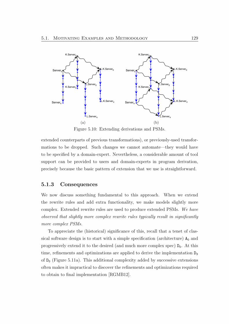
5.1. Motivating Examples and Methodology 129
Server0
K.Server0
L.Server0
L.K.Server0
Server4
K.Server4
L.Server4
L.K.Server4
(a)
Server0
K.Server0
L.Server0
L.K.Server0
Server4
K.Server4
L.Server4
L.K.Server4
(b)
Figure 5.10: Extending derivations and PSMs.
extended counterparts of previous transformations), or previously-used transfor-
mations to be dropped. Such changes we cannot automate—they would have
to be specified by a domain-expert. Nevertheless, a considerable amount of tool
support can be provided to users and domain-experts in program derivation,
precisely because the basic pattern of extension that we use is straightforward.
5.1.3 Consequences
We now discuss something fundamental to this approach. When we extend
the rewrite rules and add extra functionality, we make models slightly more
complex. Extended rewrite rules are used to produce extended PSMs. We have
observed that slightly more complex rewrite rules typically result in significantly
more complex PSMs.
To appreciate the (historical) significance of this, recall that a tenet of clas-
sical software design is to start with a simple specification (architecture) A0 and
progressively extend it to the desired (and much more complex spec) D0. At this
time, refinements and optimizations are applied to derive the implementation D3
of D0 (Figure 5.11a). This additional complexity added by successive extensions
often makes it impractical to discover the refinements and optimizations required
to obtain to final implementation [RGMB12].

130 5. Encoding Domains: Extension
A0 B0 C0 D0
D1
D2
D3
(a)
A0
A1
A2
A3
(b)
A0
A1
A2
A3
B0
B1
B2
B3
(c)
A0
A1
A2
A3
B0
B1
B2
B3
C0
C1
C2
C3
D0
D1
D2
D3
(d)
Figure 5.11: Derivation paths.
This lead us to explore an alternative, more incremental approach, based
on extensions. Instead of starting by extending the specification, we start by
obtaining an implementation for the initial specification. That is, considering
the initial specification A0, we build its derivation A0 ⇒ A1 ⇒ A2 ⇒ A3, to obtain
implementation A3 (Figure 5.11b). Next, we extend the specification, producing
a new one (B0), closer to the desired specification, from which we produce a new
derivation B0 ⇒ B1 ⇒ B2 ⇒ B3 (Figure 5.11c). We repeat the process until we
get to the final (complete) specification D0, from which we build the derivation
that produces the desired implementation D3 (Figure 5.11d).
This alternative approach makes a derivation process more incremen-
tal [RGMB12]. It allows us to start with a simpler derivation, which uses re-
finements and optimizations easier to understand and explain. Then, each new
derivation is typically obtained with rewrite rules similar to the ones used in the
previous derivation. By leveraging the relationships among the different deriva-
tions, and among the rewrite rules required for each derivation, we can improve
the development process, providing tool support to capture additional knowl-
edge, and making it easier to understand and explain. (Chapter 7 is devoted to
an analysis of the complexity of commuting diagrams like Figure 5.11d.)
The need to support extensions first appeared when reverse engineering Up-
Right [CKL+09]. Extensions allowed us to conduct the process incrementally,
by starting with a simple PIM to PSM derivation, which was progressively en-
5.2. Implementation Concepts 131
hanced until we got a derivation that produced the desired PSM [RGMB12].
Later, when analyzing other case studies, we realized that the ability to model
feature-enhanced rewrite rules was useful even to just produce different PSMs
(that only differs in non-functional properties) for the same PIM. This happens
as we add features to boxes that are not visible externally (i.e., when looking to
the entire architecture, no change on functional properties is noticed).
Road Map. In the remainder of this chapter, we outline the key ideas needed
to encode extension relationships. We explain how we capture the extension
relationships in RDMs (so that they effectively express product lines of RDMs),
and how we can leverage from the extension relationships and the methodology
proposed to provide tools support to help developers to derive product lines of
PSMs.
5.2 Implementation Concepts
5.2.1 Annotative Implementations of Extensions
There are many ways to encode extensions. At the core of ReFlO is its ability to
store rewrite rules. For each rule, we want to maintain a (small) product line of
rules, containing a base rule and each of its extensions. For a reasonable number
of features, a simple way to encode all these rules is to form the union of their
elements, and annotate each element to specify when that element is to appear
in a rule for a given set of features.
We follow Czarnecki’s annotative approach [CA05] to encode product
lines. With appropriate annotations we can express the elements that are
added/removed by extensions, so that we can “project” the version of a rule
(and even make it disappear if no “projection” remains) for a given set of fea-
tures. So in effect, we are using an annotative approach to encode extensions
and product lines of RDMs, and this allows us to project an RDM providing a
specific set of features.

132 5. Encoding Domains: Extension
Model elements are annotated with two attributes: a feature predicate and a
feature tags set. The feature predicate determine when boxes, ports, or connec-
tors are part of an RDM for a given set of features. The feature tags set is used
to determine how boxes are tagged/labeled (e.g., K is a tag for feature key).
Methodology. A user starts by encoding an initial RDM R that
allows him to derive the desired PSM from a given PIM. Then, for
each feature f ∈ F , the user considers each r ∈ R, adds the needed
model elements (boxes, ports, connectors), and annotates them to
express the f-extension of r. Doing so specifies how each rewrite rule
r evolves as each feature f is added to it. This results in a product
line of rewrite rules centered on the initial rule r and its extensions.
Doing this for all rules r ∈ R creates a product line of RDMs.
Of course, there can be 2n distinct combinations of n optional fea-
tures. Usually, when an f-extension is added, the user can take into
account all combinations of f with previous features. The rule bases
are not always complete though. Occasionally, the user may later re-
alise he needs additional rules for a certain combination of features.
5.2.2 Encoding Product Lines of RDMs
All RDMs of a product line are superimposed into a single artifact, which we
call an eXtended ReFlO Domain Model (XRDM). The structure of an XRDM is
described by the same UML class diagram metamodel previously shown (Fig-
ure 3.6). However, some objects of the XRDM have additional attributes de-
scribed below.
Boxes, ports, and connectors receive a new featuresPredicate attribute.
Given a subset of features S ⊆ F , and a model element with predicate P :
P(F) → {true, false} (where P denotes the power set), P(S) is true if and
only if the element is part of the RDM when S are the enabled features. We use
a propositional formula to specify P, where its atoms represent the features of
the domain. P(S) is computed evaluating the propositional formula associating

5.2. Implementation Concepts 133
true to the atoms corresponding to features in S, and associating false to the
remaining atoms.
Boxes have another new attribute, featuresTags. It is a set of abbreviated
features names that determines how a box is tagged. A tag is a prefix that is
added to a box name to identify the variant of the box being used (e.g., L and K
are tags of box L.K.WSERVER, specifying that this box is a variant of the WSERVER
with features L(ist) and K(ey)).2
Example: Recall our web server example. We initially defined
rewrite rule (WSERVER, pwserver) to specify a primitive implemen-
tation for WSERVER (see Figure 5.12a). Then we add feature key
(abbreviated as K) to this rewrite rule, which means adding a new
port (OK) to each box. As this port is only present when feature key
is enabled, those new ports are annotated with predicate key. More-
over, the boxes now provide extra behavior, therefore we need to add
K tag to each box. The result is depicted in Figure 5.12b (red boxes
show tags sets, and blue boxes show predicates). Finally, we add
feature list (abbreviated as L), which requires another port (OL) in
each box. Again, the new ports are annotated with a predicate (in
this case, list specifies the ports are only part of the model when
feature list is enabled). The set of tags of each box also receives an
additional tag L. The final model is depicted in Figure 5.12c.
(a)
key key{K}{K}
(b)
key key
{K,L}{K,L} list list
(c)
Figure 5.12: Incrementally specifying a rewrite rule.
2Connectors are not named elements, neither have behavior associated with them, thereforethey do not need to be tagged.
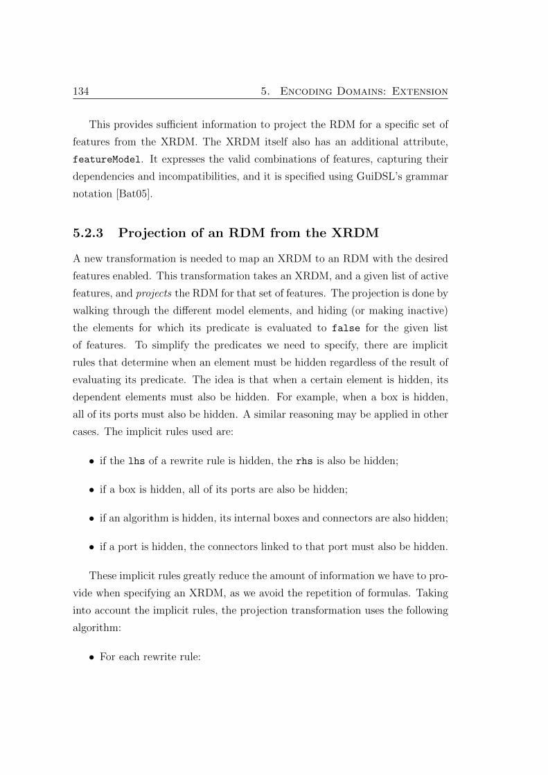
134 5. Encoding Domains: Extension
This provides sufficient information to project the RDM for a specific set of
features from the XRDM. The XRDM itself also has an additional attribute,
featureModel. It expresses the valid combinations of features, capturing their
dependencies and incompatibilities, and it is specified using GuiDSL’s grammar
notation [Bat05].
5.2.3 Projection of an RDM from the XRDM
A new transformation is needed to map an XRDM to an RDM with the desired
features enabled. This transformation takes an XRDM, and a given list of active
features, and projects the RDM for that set of features. The projection is done by
walking through the different model elements, and hiding (or making inactive)
the elements for which its predicate is evaluated to false for the given list
of features. To simplify the predicates we need to specify, there are implicit
rules that determine when an element must be hidden regardless of the result of
evaluating its predicate. The idea is that when a certain element is hidden, its
dependent elements must also be hidden. For example, when a box is hidden,
all of its ports must also be hidden. A similar reasoning may be applied in other
cases. The implicit rules used are:
• if the lhs of a rewrite rule is hidden, the rhs is also be hidden;
• if a box is hidden, all of its ports are also be hidden;
• if an algorithm is hidden, its internal boxes and connectors are also hidden;
• if a port is hidden, the connectors linked to that port must also be hidden.
These implicit rules greatly reduce the amount of information we have to pro-
vide when specifying an XRDM, as we avoid the repetition of formulas. Taking
into account the implicit rules, the projection transformation uses the following
algorithm:
• For each rewrite rule:

5.2. Implementation Concepts 135
– If the predicate of its lhs interface box is evaluated to false, hide
the rewrite rule;
– For each port of the lhs interface, if the predicate of the port is
evaluated to false, hide the port;
– If the predicate of the rhs box is evaluated to false, hide the rhs
box;
– For each port of the rhs box, if the predicate of the port is evaluated
to false, hide the port;
– If the rhs is an algorithm, for each connector of the rhs algorithm:
∗ If the predicate of the connector is evaluated to false, hide the
connector;
– If the rhs is an algorithm, for each internal box of the rhs algorithm:
∗ If the predicate of the internal box is evaluated to false, hide
the internal box;
∗ For each port of the internal box, if the predicate of the port is
evaluated to false, hide the port and the connectors linked to
the port.
During projection, we also have to determine which tags are attached to each
box. Given the set F of feature to project, and given a box B with features tags
set S, the tags of B after the projection are given by S ∩ F . That is, S specifies
the features that change the behavior of B, but we are only interested in the
enabled features (specified by F).
Example: Considering the rewrite rule from Figure 5.12c, and
assuming we want to project feature K only, we would obtain the
model from Figure 5.13. Ports OK, which depend on feature K, are
present. However, ports OL, which depend on feature L, are hidden.
Additionally, boxes are tagged with K ({K} = {K, L} ∩ {K}).

136 5. Encoding Domains: Extension
Figure 5.13: Projection of feature K from rewrite rule (WSERVER, pwserver) (notethe greyed out OL ports).
5.3 Tool Support
ReFlO was adapted to support XRDM and extensions. Besides minor changes to
the metamodels, and the addition of the RDM projection transformation, other
functionalities were added to ReFlO, namely to provide better validation, and to
help developers to replay a derivation after adding features to the RDM.
5.3.1 eXtended ReFlO Domain Models
When using extensions, we start defining an XRDM as if it was an RDM, i.e., we
specify the rewrite rules for the base (mandatory) features. Then, new elements
and annotations are incrementally added to the initial model, in order to support
other features. Typically, the new elements are annotated with a predicate that
requires the presence of the feature being defined for the element be present.
Boxes that receive new elements are also tagged. Occasionally elements previ-
ously added have their predicate changed, for example to specify they should be
removed in the presence a certain features.
Predicates are provided in featuresPredicates attribute of boxes, ports
and connectors, and are specified using a simple language for propositional for-
mulas that provides operators and (logical conjunction), or (logical disjunction),
implies (implication), and not (negation). An empty formula means true.
Tags are specified in attribute featuresTags, by providing a comma-
separated list of names. To make the tags more compact (improving the vi-
sualization of models), we allow the specification of alias that associate a shorter
tag name to a feature. Those alias are specified in attribute featuresTagsMap
of the XRDM, using a comma-separated list of pairs featurename : tagname.
The XRDM has another extra attribute, featureModel, that is used to spec-

5.3. Tool Support 137
ify the feature model of the XRDM, i.e., the valid combinations of features the
XRDM encodes. As we mentioned previously, the feature model is specified
using the language from GuiDSL [Bat05].
Given an XRDM, users can select and project the RDM for a desired set
of features. ReFlO checks whether the selected combination of features is valid
(according to the feature model), and if it is, it uses the algorithm described in
Section 5.2.3 to project the XRDM into the desired RDM.
5.3.2 Program Architectures
Developers that use ReFlO start by providing a PIM, which is progressively
transformed until a PSM with the desired properties is obtained. Given the
XRDM, the developers have to select the set of features of the RDM they want
to use to derive the PSM. Moreover, they also provide the PIM with the desired
features (often all PIMs are expressed by the same graph, where only the box
tags vary, according to the desired set of features).
Most of the variability is stored at XRDM, and when deriving a PSM, there
is already a fixed set of features selected. This means the only additional in-
formation we have to store in architectures to support extensions are box tags.
Therefore, the metamodel of architectures is modified to store this information,
i.e., boxes now have a new attribute tags.
5.3.3 Safe Composition
Dataflow models must satisfy constraints in order to be syntactically valid. ReFlO
already provided dataflow model constraint validation. Before the introduction
of extensions, it would simply assume all elements were part of the model, and
apply its validation rules (see Section 3.2.3). With extensions, the validation
function was changed to check only whether the active elements form a valid
RDM. A more important question is whether all the possible RDMs obtained
from projecting subsets of features form a valid RDM. When annotating models,

138 5. Encoding Domains: Extension
designers sometimes forget to annotate some model elements, leading to errors
that would be difficult to detect without proper tool support.3
ReFlO provides a mechanism to test if there is some product (or RDM) ex-
pressed by the SPL (XRDM) that is syntactically invalid. The implemented
mechanism is based on safe composition [CP06, TBKC07]. Constraints are de-
fined by the propositional formulas described below (built using the propositional
formulas of the model elements):4
• An implementation, if active, must have the same ports of its interface. Let
i1 be the propositional formula of the interface, and p1 be the propositional
formula of one of its ports. We know that p1⇒ i1. Let a the propositional
formula of the implementation, and p2 be the propositional formula of the
equivalent port in the implementation. The propositional formula a ⇒(p1⇔ p2) must be true.
• An interface used to define an active algorithm must be defined (i.e., it has
to be the LHS of a rewrite rule). Let i2 be the propositional formula of the
interface used to define the algorithm, and i1 be the propositional formula
of the interface definition. The propositional formula i2 ⇒ i1 must be
true.
• An algorithm must have the same ports as its interface (i.e., the LHS
and RHS of a rewrite rule must have the same ports). Let p3 be the
propositional formula of a port of an interface used to define an algorithm,
i2 be the propositional formula of the interface, and p1 be the propositional
formula of the same port in the interface definition. The propositional
formula i2⇒ (p1⇔ p3) must be true.
• The input ports of interfaces used to define an algorithm must have one
and only one incoming connector. Let p3 be the propositional formula of
3In our studies, we noticed that we sometimes forget to annotate ports that are added fora specific feature.
4We refer to the explicit propositional formula defined in the model elements in conjunctionwith their implicit propositional formulas, as defined in Section 5.2.3.

5.3. Tool Support 139
an input port of an interface used to define an algorithm, and c1, . . . , cn be
the propositional formulas of its incoming connectors. The propositional
formula p3⇒ choose1(c1, . . . , cn)5 must be true.
• The output ports of an algorithm must have one and only one incoming
connector. Let p4 be the propositional of an output port of an algorithm,
and c1, . . . , cn be the propositional formulas of its incoming connectors.
The propositional formula p4⇒ choose1(c1, . . . , cn) must be true.
Let fm be the feature model propositional formula. To find combinations of
features that originate an invalid RDM, for each of the propositional formulas p
described above, and for each model element it applies to, we test the proposi-
tional formula fm∧¬p with a SAT solver.6 If there is a combination of features for
which one of those predicates is true, then that combination of features reveals
an invalid RDM. ReFlO safe composition test tells the developer if there is such
combination, and, in case it exists, the combination of features and the type of
problem detected. Given a combination that produces the invalid RDM, the de-
veloper may use ReFlO to project that features and validate the obtained RDM
(doing this, the developer obtains more precise information about the invalid
parts of the RDM, which allows him to fix them).
In addition, ReFlO can also detect bad smells, i.e., situations that, although
do not invalidate an RDM, are uncommon and likely to be incorrect. The two
case we detect are:
• The input of an algorithm is not used (i.e., a dead input). Let p be the
propositional formula of an input port of an algorithm, and c1, . . . , cn be
the propositional formulas of its outgoing connectors. The propositional
formula p⇒ choose(c1, . . . , cn) must be true.
5choose(e1, . . . , en) means at least one of the propositional formula e1, . . . , en is true, andchoose1(e1, . . . , en) means exactly one of the propositional formulas e1, . . . , en is true [Bat05].
6Although SAT solvers may imply a significant performance impact in certain uses, in thisparticular kind of application, for the most complex case study we modeled (with 4 differentfeatures, and about 40 rewrite rules) the test requires less than 2 seconds to run.
140 5. Encoding Domains: Extension
• The output of an interface in an algorithm is not used (i.e., a dead output).
Let p be the propositional formula of an output port of an interface used
to define an algorithm, and c1, . . . , cn be the propositional formula of its
outgoing connectors. The propositional formula p ⇒ choose(c1, . . . , cn)
must be true.
In case there is a combination of features where a bad smell is detected, the
developer is warned, so that he can further check if the XRDM is correct.
5.3.4 Replay Derivation
When reverse engineering existing programs using ReFlO extensions, we start
with a minimal PIM and an RDM with minimal features, and the PIM is mapped
to a PSM. Later, an RDM and PIM with additional features is used, to produce a
new derivation of a PSM that is closer to the desired implementation. This new
derivation usually reuses the same transformations (or rather their extended
counterparts) to produce the PSM. Sometimes new transformations are also
required, or previously used transformations are not needed anymore.
Therefore, it is important to keep track of the sequence of transformations
used in a derivation, as it can be used to help producing a new derivation. ReFlO
stores the list of transformations used in a derivation. In this way, when trying
to obtain a derivation of PIM with a different set of features, developers can ask
ReFlO to replay the derivation. The user should select both the new PIM and the
previously derived PSM. ReFlO reads the transformations used in the previously
derived PSM, and tries to reapply the same sequence of transformation to the
new PIM.7 As mentioned earlier, new transformations may be needed (typical
when we added features to the PIM), or certain transformations may not be ap-
plicable anymore (typical when we remove features from the PIM). ReFlO stops
the replay process if it reaches a transformation it cannot successfully reapply,
either because is not needed anymore, or because an entirely new transforma-
tion is required in the middle of the derivation. After this point, the developer
7Box names do not change, they are only tagged. In this way it is easy to determine theextended counterpart of a transformation used in a previous derivation.

5.3. Tool Support 141
has to manually apply the remaining transformations, in case there are more
transformations needed to finish the derivation.


Chapter 6
Extension Case Studies
To validate our approach to encode extensions and product lines, we used ReFlO
on different case studies. This chapter is dedicated to two of those case stud-
ies. We start with a case study where a fault-tolerant server architecture is
reverse-engineered using extensions and our incremental approach. Later we
show another case study where different variants of an MD simulation program
are derived with the help of extensions.
6.1 Modeling Fault-Tolerant Servers
UpRight [CKL+09] is a state-of-the-art fault-tolerant server architecture. It
is the most sophisticated case study to which we applied extensions, and its
complexity drove us to develop its architecture incrementally, using extensions,
thereby creating a small product line of UpRight designs. The initial architec-
ture SCFT defines a vanilla RPA. Using refinements and optimizations, we show
how this initial program architecture is mapped to a PSM that is fault-tolerant.
Later, extensions (features) are added to provide recovery and authentication
support. Figure 6.1 shows the diagram of the product line that is explored in
this section.
We start with the initial PIM of UpRight.
143

144 6. Extension Case Studies
SCFT
R.SCFT
A.SCFT
A.R.SCFT
Figure 6.1: The UpRight product line.
6.1.1 The PIM
The initial PIM for this architecture is depicted in Figure 6.2a. It contains
clients (C boxes) that send requests to a server.1 The requests are first serialized
(Serial box), and then sent to the server (VS box). The server processes each
request in order (which involves updating the server’s state, i.e., the server is
stateful), and outputs a response. The response is demultiplexed (Demult box)
and sent back to the client that originated the request. The program follows
a cylinder topology, and the initial PIM is in fact the result of unrolling the
cylinder depicted in Figure 6.2b.
(a) (b)
Figure 6.2: The PIM.
6.1.2 An SCFT Derivation
The simplest version of UpRight implements a Synchronous Crash-Fault Tolerant
(SCFT) server, which has the ability to survive to failures of some components.
The design removes single points of failure (SPoF), i.e., boxes that if they failed
(stopped processing requests altogether), they would make the entire server ab-
1For simplicity, we have only two clients in the PIM. There may exist any number of clients;our approach/tools supports its representation using replication.

6.1. Modeling Fault-Tolerant Servers 145
straction fail. For example, in the PIM, boxes Serial, VS and Demult are SPoF.
In this derivation, we show how SPoF are eliminated by replication [Sch90].
Figure 6.3: list algorithm.
The derivation starts by refining the VS box,
to expose a network queue in front of the server.
The list algorithm, depicted in Figure 6.3, is
used. This refinement places an L box (list or
queue) between the clients and the server, which
collects the requests sent by clients, and passes
them to the server, one at the time. The architecture obtained is depicted in
Figure 6.4.
Figure 6.4: SCFT after list refinement.
Figure 6.5: paxos algorithm.
Next, the network
queue and the server are
replicated, using a map-
reduce strategy, to in-
crease resilience to crashes
of those boxes. The paxos
algorithm (Figure 6.5)
replicates the network
queue [Lam98]. This algorithm forwards the input requests to different agree-
ment boxes A, that decide which request should be processed next.2 The requests
are then serialized and sent to the quorum box (Qa), which outputs the request
as soon as it receives it from a required number of agreement boxes.
2As for clients, we use only two replicas for simplicity. The number of replicas depends onthe number of failures to tolerate. The number of clients, agreement boxes and servers is notnecessarily the same.

146 6. Extension Case Studies
Figure 6.6: reps algorithm.
The reps algorithm
(Figure 6.6) replicates the
server. The algorithm re-
liably broadcasts (RBcast)
requests to the server repli-
cas. For correctness, it is
important to guarantee that
all servers receive each request in synchrony, thus the need for the reliable broad-
casts. The servers receive and process the requests in lock step, their responses
are serialized and sent to the quorum box (Qs) that outputs the response as
soon as it receives the same response from a required number of servers. The
architecture obtained is depicted in Figure 6.7.
Figure 6.7: SCFT after replication refinements.
Figure 6.8: Rotation optimization.
At this point, although
we improved the resilience to
crashes of the server, the en-
tire system contains even more
SPoF than the original (there
were originally 3 SPoF, and
now we have 8 SPoF). We
rely on optimizations to re-
move them. Rotation opti-
mizations, which swap the or-
der in which two boxes are
composed, remove SPoF.
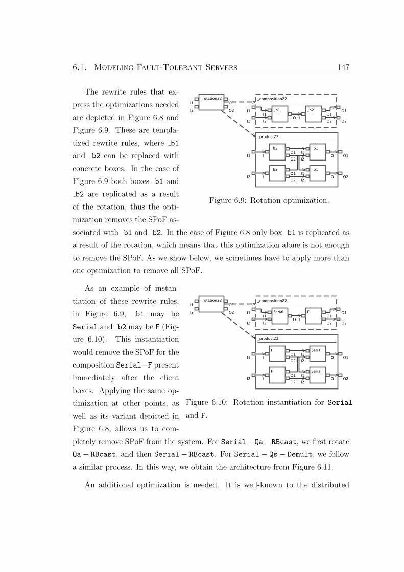
6.1. Modeling Fault-Tolerant Servers 147
Figure 6.9: Rotation optimization.
The rewrite rules that ex-
press the optimizations needed
are depicted in Figure 6.8 and
Figure 6.9. These are templa-
tized rewrite rules, where b1
and b2 can be replaced with
concrete boxes. In the case of
Figure 6.9 both boxes b1 and
b2 are replicated as a result
of the rotation, thus the opti-
mization removes the SPoF as-
sociated with b1 and b2. In the case of Figure 6.8 only box b1 is replicated as
a result of the rotation, which means that this optimization alone is not enough
to remove the SPoF. As we show below, we sometimes have to apply more than
one optimization to remove all SPoF.
Figure 6.10: Rotation instantiation for Serial
and F.
As an example of instan-
tiation of these rewrite rules,
in Figure 6.9, b1 may be
Serial and b2 may be F (Fig-
ure 6.10). This instantiation
would remove the SPoF for the
composition Serial−F present
immediately after the client
boxes. Applying the same op-
timization at other points, as
well as its variant depicted in
Figure 6.8, allows us to com-
pletely remove SPoF from the system. For Serial−Qa−RBcast, we first rotate
Qa− RBcast, and then Serial− RBcast. For Serial− Qs− Demult, we follow
a similar process. In this way, we obtain the architecture from Figure 6.11.
An additional optimization is needed. It is well-known to the distributed

148 6. Extension Case Studies
Figure 6.11: SCFT after rotation optimizations.
systems community that reliable broadcast is expensive, and therefore should be
avoided. As quorums are taken from the requests broadcast, reliable broadcasts
can be replaced by simple (unreliable) broadcasts. (Although this step may not
be obvious for readers, it is common knowledge among domain experts.) After
this step, we obtain the desired SCFT architecture, depicted in Figure 6.12. This
is the “big-bang” design that was extracted by domain experts from UpRight’s
implementation.
Figure 6.12: The SCFT PSM.
6.1.3 Adding Recovery
There are other features we may want to add to our initial PIM. The SCFT
implementation previously derived improved resilience to failures. Still, a box
failure would be permanent, thus, after a certain amount of failures, the entire
system would fail.
The resilience to failures can be further improved adding recovery capabilities,
so that the system can recover from occasional network asynchrony (e.g., box
failures). We now show how the RDM used in the SCFT can be extended so
that an enhanced implementation of the SCFT with recovery capabilities, called
Asynchronous Crash-Fault Tolerant (ACFT), can be derived.
The first step is to Recovery-extend the SCFT PIM to the ACFT PIM. That
is, we want to show SCFT R.SCFT, where ACFT = R.SCFT. The ACFT PIM is

6.1. Modeling Fault-Tolerant Servers 149
shown in Figure 6.13. Our goal is to map it to its PSM by replaying the SCFT
derivation using Recovery-extended rewrite rules.
Figure 6.13: The ACFT PIM.
{R} {R}
Recovery Recovery
Figure 6.14: list algorithm,
with recovery support.
As for SCFT, the first step in the ACFT
derivation is a refinement that exposes a net-
work queue in front of the server. The algo-
rithm has to be extended to account for recov-
ery. Boxes L and S are both extended so that
S can send recovery information to L. Thus,
tag R is added to the tags set of both boxes. S
gets a new output port that produces recovery
information, and L gets a new input port that
receives this information. Moreover, a new connector is added in algorithm list,
linking the new ports of S and L. The new ports are annotated with the predicate
Recovery, as they are only part of the RDM when we want the recovery prop-
erty. The result is the algorithm depicted in Figure 6.14.3 Using the extended
algorithm to refine the initial specification, we obtain the architecture shown in
Figure 6.15.
The next transformations in the ACFT derivation are the replication of boxes
L and S. Again, the algorithms previously used have to be extended to account
for recovery.
3Tags sets are not graphically visible in an XRDM. This happens as the XRDM expressesall combinations of features, and the tags sets contains tags for features that change thebehavior of a box, namely for feature that may not be “enabled” in a particular derivation.Architectures, on the other hand, have a fixed set of features, therefore tags are graphicallyvisible. In the figures of XRDM boxes, we use red boxes to show tags sets attribute, and blueboxes to show predicates attribute.

150 6. Extension Case Studies
Figure 6.15: ACFT after list refinement.
{R}
RecoveryRecovery Recovery
Figure 6.16: paxos algorithm, with recovery support.
For paxos, a new input
port is added (to match
interface L). The A boxes
are also extended with
an equivalent input port.
Thus, tag R is added to the
tags set of box A. Addi-
tionally, a new RBcast box
is added, as well as the ap-
propriate connectors, to broadcast the value of the new input port of paxos to
the new inputs ports of A. The new ports of paxos and A, as well as box RBcast,
are annotated with predicate Recovery. The extended algorithm is depicted in
Figure 6.16.
{R}
Recovery Recovery Recovery Recovery
Figure 6.17: rreps algorithm, with recovery support.
For reps, a new out-
put port is added to
the algorithm box. As
mentioned earlier, S also
has an additionally out-
put port that provides the
values for the new output
port of the algorithm. The
values are first serialized
(Serial), and then sent to a quorum box (Qr), before being output. The new
ports of reps and S, and boxes Serial and Qr are annotated with predicate
Recovery. The appropriate connectors are also added. Tag R is added to the
tags set of box S. The extended algorithm is depicted in Figure 6.17.

6.1. Modeling Fault-Tolerant Servers 151
Fig
ure
6.18
:ACFT
afte
rre
plica
tion
refinem
ents
.

152 6. Extension Case Studies
Note that interface Qr did not exist before. This is an example of a case
where new rewrite rules need to be added to the RDM, as part of an extension,
to handle new interfaces. Applying the refinements again, we obtain the program
depicted in Figure 6.18.
We have now reached the point where we have to use optimizations to remove
SPoF. Optimizations do not affect extended boxes, and therefore the optimiza-
tion rewrite rules do not need to be extended. We can just reapply their previous
definitions. Doing so, we obtain the architecture depicted in Figure 6.19.
Figure 6.19: ACFT after replaying optimizations.
Nevertheless, in this case previous optimizations are not enough. We need to
apply additional optimizations to the composition of boxes Serial−Qr−RBcast,
which are still SPoF in the architecture of Figure 6.19. The aforementioned com-
position of boxes can optimized also using rotations, similarly to the optimization
of Serial− Qa− RBcast. After these optimizations we obtain the architecture
depicted in Figure 6.20, with no SPoF, i.e., the PSM for the ACFT program.
Figure 6.20: The ACFT PSM.

6.1. Modeling Fault-Tolerant Servers 153
6.1.4 Adding Authentication
We saw earlier how the recovery feature mapped UpRight’s SCFT design, its
derivation and rewrites to UpRight’s ACFT design, its derivation and rewrites.
We now show how the ACFT server can be extended with another property,
Authentication, which is the next stage in UpRight’s design. This new system,
called AACFT (AACFT = A.R.SCFT), changes the behavior of the system by check-
ing the requests and accepting only those from valid clients. That is, the server
has now also validation capabilities, and therefore box R.VS receives a new tag
to express this new feature (producing box A.R.VS). The initial PIM for this new
derivation is shown in Figure 6.21.
Figure 6.21: The AACFT PIM.
{A,R} {R}
Recovery RecoveryAuthenticationnot Authentication
Figure 6.22: list algorithm, with recovery
and authentication support.
We now replay the ACFT
derivation to obtain the desired
implementation (PSM). The
list algorithm is A-extended,
to support authentication (Fig-
ure 6.22). This extension of list
requires a box V, which validates
and filters requests, to be added
before the network queue. The
new box is annotated with predicate Authentication. This also means
the previous connector that links input I of list to input I of L is not
present when authentication is being used (thus, it is annotated with predi-
cate not Authentication). After performing this refinement, the architecture
from Figure 6.23 is produced.

154 6. Extension Case Studies
Figure 6.23: AACFT after list refinement.
Figure 6.24: repv algorithm.
The previous replication al-
gorithms are not affected by
this new feature. However, a
new replication refinement is
needed, to handle the new box
V. For that purpose, we use the
algorithm repv (Figure 6.24)
to replicate V boxes using a map-reduce strategy, similar to the algorithm reps.
That is, input requests are broadcast, and after being validated in parallel, they
are serialized, and a quorum is taken. The resulting architecture is depicted in
Figure 6.25.
For the optimization step, we replay the optimizations used in the ACFT
derivation. However, the sequential composition of boxes Serial−F is no longer
present, which means the optimization that removes these SPoF is not applicable
anymore. Instead, we have two new groups of boxes forming SPoF: (i) Serial−Bcast, and (ii) Serial − Qv − F (Figure 6.26). Rotations are once again used
to remove these SPoF, allowing us to produce the desired PSM, depicted in
Figure 6.27.
6.1.5 Projecting Combinations of Features: SCFT with
Authentication
We have enhanced the XRDM specifying extensions to support recovery and
authentication, besides the base fault-tolerance property. With only the infor-
mation already provided in the XRDM, there is yet another implementation we
can derive: SCFT with authentication, or ASCFT = A.SCFT. We can project

6.1. Modeling Fault-Tolerant Servers 155
Fig
ure
6.25
:AACFT
afte
rre
plica
tion
refinem
ents
.
Fig
ure
6.26
:AACFT
afte
rre
pla
yin
gop
tim
izat
ions.
Fig
ure
6.27
:T
heAACFT
PSM
.

156 6. Extension Case Studies
the RDM that expresses the desired features, and replay the derivation to ob-
tain the implementation of ASCFT. The rewrite rules used for refinements, after
projected, result in the graphs depicted in Figure 6.28.
(a) (b)
(c)
(d)
Figure 6.28: Rewrite rules used in initial refinements after projection (note thegreyed out hidden elements, which are not part of the model for the currentcombination of features).
Figure 6.29: The ASCFT PIM.
Given the initial PIM for ASCFT (Figure 6.29), ReFlO is able to replay the
derivation automatically (this derivation requires only a subset of the transforma-
tions used for the AACFT derivation), and produce the desired implementation,
depicted in Figure 6.30.

6.1. Modeling Fault-Tolerant Servers 157
Fig
ure
6.30
:T
heASCFT
PSM
.

158 6. Extension Case Studies
Figure 6.2
Figure 6.13
Figure 6.29
Figure 6.21
Figure 6.12
Figure 6.20
Figure 6.30
Figure 6.27
RA
A R
Figure 6.31: UpRight’s extended derivations.
Recap. We showed how different designs of UpRight were obtained using the
approach we propose. By using extensions we were able to encode and expose
deep domain knowledge used to build such designs. We derived an optimized
implementation that provides fault-tolerance. Later we improved fault-tolerance
by adding recovery capabilities, and we also added authentication support. For
the different combinations of features, we were able to reproduce the derivation.
Figure 6.31 illustrates the different derivations covered in this section.
6.2 Modeling Molecular Dynamics Simulations
Another case study we explored to validate our work was MD simulations.
The base implementation was the Java Grande Forum benchmark implemen-
tation [BSW+99], to which several other improvements are applied [SS11]. This
implementation provides the core functionality of the most computationally in-
tensive part of an MD simulation.
In this section we show how we can model a small product line of MD pro-
grams. The base PIM is mapped to optimized parallel implementations. Ex-
tensions are used to add further improvements, such as Neighbors, Blocking, and
Cells [SS11]. Figure 6.32 shows the diagram of the product line that is explored

6.2. Modeling Molecular Dynamics Simulations 159
in this section (note that the Cells feature requires the Blocks feature).
MD
N.MD
B.MD
B.N.MD
C.B.MD
C.B.N.MD
Figure 6.32: The MD product line.
6.2.1 The PIM
MD simulations are typically implemented by an iterative algorithm. A list of
particles is updated at each iteration, until the particles stabilize, and some
computations are then done using the updated list of particles. The architecture
for the loop body of the program used is depicted in Figure 6.33, where we
have the UPDATEP that updates the particles (input/output p), and some other
additional operations to compute the status of the simulation.
Figure 6.33: MD loop body.
The most important part of the algorithm is the update of particles, as it is
computationally intensive, and contains the boxes that are affected by transfor-
mations. Therefore, in this section we use the architecture depicted in Figure 6.34
(that we call MDCore) as PIM. Besides input/output p, we also have input/output
epot (potential energy) and vir (virial coefficient).

160 6. Extension Case Studies
Figure 6.34: The MDCore PIM.
6.2.2 MD Parallel Derivation
We start by showing the derivation that maps the initial PIM to a parallel
implementation. Different choices of algorithms can be used to target the PIM
to different platforms, namely shared memory, distributed memory, or both.
We obtain the implementation that uses both shared and distributed memory
parallelization at the same time (the other two implementations can be obtained
removing one of the refinements used). The distributed memory parallelization
follows the SPMD model, where replicas of the program run on each processes.
All data is replicated in all processes, but each process only deals with a portion
of the total computation.
Figure 6.35: move forces algorithm.
The derivation starts by applying a
refinement that exposes the two steps of
updating the list of particles. The al-
gorithm used (depicted in Figure 6.35),
shows how the two steps are composed.
First the particles are moved (box MOVE),
based on the current forces among the
particles. Then the forces are recomputed based on the new positions of the
particles (box FORCES). This results in the architecture depicted in Figure 6.36.
The next step is to parallelize the operation FORCES for distributed memory
platforms, as shown in the algorithm depicted in Figure 6.37. The algorithm
starts by dividing the list of particles, so that each process (program replica) only
computes a subset of the forces [BSW+99]. This is done by box PARTITION, which
takes the entire set of particles, and outputs a different (disjoint) subset on each
program replica. In fact, the division of particles is only logical, and all particles
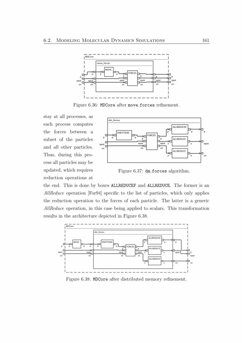
6.2. Modeling Molecular Dynamics Simulations 161
Figure 6.36: MDCore after move forces refinement.
Figure 6.37: dm forces algorithm.
stay at all processes, as
each process computes
the forces between a
subset of the particles
and all other particles.
Thus, during this pro-
cess all particles may be
updated, which requires
reduction operations at
the end. This is done by boxes ALLREDUCEF and ALLREDUCE. The former is an
AllReduce operation [For94] specific to the list of particles, which only applies
the reduction operation to the forces of each particle. The latter is a generic
AllReduce operation, in this case being applied to scalars. This transformation
results in the architecture depicted in Figure 6.38.
Figure 6.38: MDCore after distributed memory refinement.

162 6. Extension Case Studies
Figure 6.39: sm forces algorithm.
The derivation is
concluded with paral-
lelization of FORCES for
shared memory plat-
forms, using the algo-
rithm depicted in Fig-
ure 6.39. This paral-
lelization is similar to the one used before for distributed memory. It also starts
by dividing the list of particles. However, in this case, the forces of particles are
physically copied to a different memory location, specific to each thread. This
is done by box SMPARTITION. As the data is moved, the forces computation has
to take into account the new data location, thus a different SMFORCES operation
is used. Additionally, this operation also has to provide proper synchronization
when updating epot and vir values (that store the global potential energy and
virial coefficient of the simulation), which are shared among all threads. In the
end, the data computed by the different threads has to be joined, and moved
backed to the original location. This is done by box REDUCEF, which implements
a Reduce operation. epot and vir do not need to be reduced, as their values
are shared among all threads. This transformation results in the architecture
depicted in Figure 6.40, or equivalently the flattened architecture in Figure 6.41.
Figure 6.40: MDCore after shared memory refinement.
6.2.3 Adding Neighbors Extension
One common optimization applied to MD simulations consists in pre-computing
(and caching) the list of particles that interact with any other particle [Ver67].

6.2. Modeling Molecular Dynamics Simulations 163
Figure 6.41: The MDCore PSM.
This improves performance as forces between particles that are not spatially close
can be ignored, therefore by caching the pairs that interact we can reduce the
O(N2) complexity. We call this optimization Neighbors, as this pre-computation
essentially determines the neighbors of each particle. This optimization may
or may not change the behavior of the simulation,4 but we still use extensions
to model this optimization, as it requires the extension of the behavior of the
internal boxes used by the program.
The starting point for this derivation is the Neighbors-extended PIM (called
NMDCore), depicted in Figure 6.42, which uses the tagged UPDATEP operation.
Figure 6.42: The NMDCore PIM.
From this PIM, we replay the previous derivation, starting with the
move forces algorithm. The algorithm is extended as shown in Figure 6.43,
in order to support the Neighbors feature. Box NEIGHBORS, which does
the pre-computation, is added. Box FORCES is extended to take into ac-
count the data pre-computed by NEIGHBORS, and receives a new input
port (N). The appropriate connectors are also added, to provide the list
of particles to NEIGHBORS, and to provide the neighbors data to FORCES.
4If we “relax” the correction criteria of the simulation (and therefore change the behaviorof the program), we can improve performance.

164 6. Extension Case Studies
{N}
NeighborsNeighbors
Figure 6.43: move forces algorithm, with neighbors
support.
As the behavior of FORCES
changes, tag N is added to
the tags set of this box.
The new box and the new
input port are annotated
with predicate Neighbors,
to denote that they are
only part of the model
when we want the neigh-
bors feature. This transfor-
mation results in the architecture depicted in Figure 6.44.
Figure 6.44: NMDCore after move forces refinement.
NeighborsNeighbors
{N}
Figure 6.45: dm forces algorithm, with neighbors support.
We proceed with
the transformations
to parallelize the
FORCES operation.
First we add dis-
tributed memory
parallelism, by us-
ing the dm forces
algorithm. As the
FORCES operation
was extended, we
have to extend their implementations too. Figure 6.45 depicts the Neighbors-

6.2. Modeling Molecular Dynamics Simulations 165
extended dm forces algorithm. Essentially, we need to add the new input
port N to the algorithm box and to the FORCES box, and a connector linking
these two ports is added. The new input ports are annotated with predicate
Neighbors. As we mentioned before, N is added to the tags set of FORCES. This
transformation results in the architecture depicted in Figure 6.46.
Figure 6.46: NMDCore after distributed memory refinement.
Figure 6.47: Swap optimization.
With the previous
refinement, although we
only apply the FORCES
operation to a subset of
the particles (the op-
eration appears after
the PARTITION opera-
tion), the same does
not happens with the
NEIGHBORS operation
that is applied to the
full set of particles, even though only a subset is need, and therefore this opera-
tion is not parallelized. However, a simple optimization can be used to swap the
order of the PARTITION and the NEIGHBORS operations (when both operations
appear immediately before a FORCES operation). This optimization is expressed
by the templatized rewrite rules depicted in Figure 6.47. Boxes part and
forces may either be PARTITION and FORCES, or SMPARTITION and SMFORCES
(i.e., this optimization can also be used to optimize an inefficient composition

166 6. Extension Case Studies
of boxes that results from the shared memory refinements, as we will see later).
This optimization results in the architecture depicted in Figure 6.48.
Figure 6.48: NMDCore after distributed memory swap optimization.
NeighborsNeighbors
{N}
Figure 6.49: sm forces algorithm, with neighbors support.
Next we ap-
ply the refinement
for shared mem-
ory parallelization.
The algorithm used
in this refinement
(sm forces) needs
to be extended in
a similar way to
dm forces, so that it supports the Neighbors feature. It is depicted in Fig-
ure 6.49. This transformation results in the architecture depicted in Figure 6.50.
Figure 6.50: NMDCore after shared memory refinement.
We need again to use the swap optimization so that the neighbors are com-
puted in parallel too. As we saw before, the optimization from Figure 6.47 can
also be applied in the architecture from Figure 6.50 (after flattening it), yielding
the architecture depicted in Figure 6.51.

6.2. Modeling Molecular Dynamics Simulations 167
Figure 6.51: The NMDCore PSM.
6.2.4 Adding Blocks and Cells
When the set of particles is large enough to not fit in cache, there are additional
optimizations that may be made to the program [YRP+07]. The use of a cache
can be improved by using algorithms by Blocks, which divide the set of particles in
blocks that fit into the cache (similarly to the blocked algorithms used in DLA).
This feature does not really change the structure of the algorithm; we simply need
to use boxes that are prepared to deal with a list of blocks of particles, instead
of a list of particles. Thus, the optimized architecture is obtained replaying the
previous derivation, but now some boxes have an additional tag B. The final
architecture is depicted in Figure 6.52.
Figure 6.52: The BNMDCore PSM (NMDCore with blocks).
The blocks feature is important as it enables yet another optimization, which
we call Cells [SS11]. Whereas the blocks feature just divides the list of particles
in blocks randomly, the cells feature rearranges the blocks so that the particles in
each block are spatially close, i.e., the division in blocks is not random anymore.
As particles interact with other particles that are spatially close to them, by
rearranging the division of particles, for a given particle, we can reduce the list

168 6. Extension Case Studies
of particles we have to check (to decide whether there will be interaction) to those
particles that are in blocks spatially close to the block of the given particle. When
we have the Neighbors feature, the same reasoning may be applied to optimize
the computation of the neighbors list.
The starting point for this derivation is the PIM extended with features
Neighbors, Blocks, and Cells (called CBNMDCore), depicted in Figure 6.53, that
uses the UPDATEP operation tagged with C, B, and N.
Figure 6.53: The CBNMDCore PIM.
{C,B,N}
NeighborsNeighborsCells not Cells
{C,B}{B}
Figure 6.54: move forces algorithm, with support for
neighbors, blocks and cells.
From this PIM,
we replay the pre-
vious derivation, us-
ing the move forces
algorithm. This al-
gorithm is extended
again, as shown in
Figure 6.54. Box
PSORT is added to re-
arrange the list of
blocks of particles
after moving the particles. These new rearranged list of blocks must then be
used by boxes NEIGHBORS and FORCES. Thus, new connectors link the output
of PSORT with NEIGHBORS and FORCES. Boxes NEIGHBORS and FORCES receive
an additional tag C. The new PSORT box is annotated with predicate Cells.
Additionally, the old connectors providing the list of blocks to boxes NEIGHBORS
and FORCES shall not be used when this feature is enabled, therefore those con-
nectors are annotated with predicate not Cells. This transformation produces
the architecture depicted in Figure 6.55.

6.2. Modeling Molecular Dynamics Simulations 169
Figure 6.55: CBNMDCore after move forces refinement.
We proceed with the transformations to parallelize the FORCES operation.
First we add distributed memory parallelism, by using the dm forces algorithm
and swap optimization. Then we add shared memory parallelism, by using the
sm forces algorithm and the swap optimization again. Other than adding tag
C to boxes NEIGHBORS, FORCES, PARTITION, and SMPARTITION, there is no other
change to the (X)RDM. After we reapply the transformations we obtain the
architecture depicted in Figure 6.56, which is the final PSM.
Figure 6.56: The CBNMDCore PSM.
Recap. We showed how we can encode the knowledge needed to obtain dif-
ferent MD simulations programs. We derived optimized implementations that
use shared and distributed memory parallelism, and we showed how we can ob-
tain four variants (with different optimizations) of the program for this target
platform. Figure 6.57 illustrates the different derivations covered in this section.
Even though we only show derivations for one target platform, by removing
some transformations from the derivation, we would be able to target shared
memory platforms, and distributed memory platforms (individually). Moreover,
besides the four combinations of features illustrated in this section, there are
two other combinations of features we could use (as shown in Figure 6.32, we

170 6. Extension Case Studies
Figure 6.41
Figure 6.51
Figure 6.34
Figure 6.42
Figure 6.53
Figure 6.56
Figure 6.52
NB
C
C
B N
N
Figure 6.57: MD’s extended derivations.
could also use combination of features B.MDCore, and C.B.MDCore). This means
the knowledge encoded in the XRDM used for MD is enough to obtain a total
of 18 optimized architectures (PSMs), targeting different platforms, and provid-
ing different features (optimizations), which users can enable according to their
needs. That is, they can take advantage of a certain feature if the problem they
have at hands benefits from using that feature, but they also avoid the downsides
of the feature (overheads, load balancing problems, etc.) if the feature does not
provide gains to compensate the downsides in a particular simulation.
The same set of PSMs could be obtained using refinements only. However,
it would required multiple variants of algorithms to be modeled separately (for
example, we would need the 6 different variants of move forces algorithm to
be modeled individually), leading to replicated information, which complicates
development and maintenance.
Chapter 7
Evaluating Approaches with
Software Metrics
We believe derivational explanations of dataflow designs are easier to understand
and appreciate than a big-bang presentation of the final graph. Controlled ex-
periments have been conducted to test this conjecture. The first experiments,
which tried to measure (compare) the knowledge of the software acquired by
users when exposed to the big-bang design and when exposed to the derivation,
were inconclusive and did not show a significative advantage or disadvantage of
using a derivational approach [FBR12]. Additional controlled experiments were
conducted to determine the users perception of the derivational approach, to
find out which method users (in this case, Computer Science students) prefer,
and which method they think is better to implement, maintain, and comprehend
programs. In this study, students showed a strong preference for the use of a
derivational approach [BGMS13]. Despite some comments that the derivational
approach has, in certain cases, too much overhead, and that such overhead is
unjustifiable if the big-bang design is simple enough to be understood as a whole,
the large majority of users comments were favorable to the derivational approach.
Users pointed that the derivational approach allows them to divide the problem
is smaller pieces, easier to understand, implement, and extend. Users also noted
that the structure used to encode knowledge makes it easier to test the individual
171

172 7. Evaluating Approaches with Software Metrics
components of the program, and detect bugs earlier.
In this chapter we report an alternative (and supportive) study based on
standard metrics (of McCabe and Halstead) to estimate the complexity of source
code [Hal72, Hal77, McC76]. We adapt these metrics to estimate the complexity
of dataflow graphs and to understand the benefits of DxT derivations of dataflow
designs w.r.t. big-bang designs—where the final graph is presented without en-
coding/documenting its underlying design decisions.
7.1 Modified McCabe’s Metric (MM)
McCabe’s cyclomatic complexity is a common metric of program complex-
ity [McC76]. It counts the linearly independent paths of a graph that represent
the control flow of a program. This metric is important in software testing as it
provides the minimum number of test cases to guarantee complete coverage.
We adapted this metric to measure the complexity and effort to understand
dataflow graphs. Our metric measures the length (number of boxes) of a maximal
set of linearly independent paths of a dataflow graph. Cyclomatic complexity
captures the structure of the graph by considering all linearly independent paths
(which basically increases as more outgoing edges are added to boxes). Our
intuition goes beyond this to say that the number of boxes in a path also impacts
the effort needed to understand it. Hence, our metric additionally includes the
path length information.
We abstract DxT graphs to simple multigraphs by ignoring ports. For exam-
ple, the dataflow graph of Figure 7.1a is abstracted to the graph of Figure 7.1b.
(a)
I
IL
SPLITMERGE
PROJECT
PROJECT*O
(b)
Figure 7.1: A dataflow graph and its abstraction.
7.1. Modified McCabe’s Metric (MM) 173
The graph from Figure 7.1b has 4 linearly independent paths:
• I→ SPLIT→ PROJECT→ MERGE→ O
• I→ SPLIT→ PROJECT∗ → MERGE→ O
• IL→ PROJECT→ MERGE→ O
• IL→ PROJECT∗ → MERGE→ O
The sum of the lengths of (number of interface nodes in) each path is 3+3+2+2 =
10. This is our measure of the complexity of the dataflow graph of Figure 7.1a.
The complexity of a set of graphs is the sum of the complexity of each graph
present in the set. The complexity of a derivation is the complexity of a set of
graphs that comprise (i) the initial dataflow graph of the program being derived,
and (ii) the RHS of the rewrite rules used in the derivation. If the same rewrite
rule is used more than once in a derivation, it is counted only once (as the rewrite
rule is defined once, regardless of the number of times it is used).1
As an example, consider the derivation in Figure 7.2, previously discussed
in Section 3.1. Figure 7.2e shows the final graph, which can be obtained incre-
mentally transforming the initial graph shown in Figure 7.2a. From Figure 7.2a
to Figure 7.2b, algorithms parallel project and parallel sort are used to
refine PROJECT and SORT, respectively. From Figure 7.2b to Figure 7.2c we re-
move the modular boundaries of the algorithms previously introduced. From
Figure 7.2c to Figure 7.2d we replace the subgraph identified by the dashed red
lines, using the optimization specified by the rewrite rules previously depicted in
Figure 3.13. After flattening Figure 7.2d, the final graph is obtained.
We measure the complexity of this derivation to be: 2 (initial graph) + 3
+ 3 (parallel project) + 3 + 3 (parallel sort) + 2 + 2 + 2 + 0 + 0
(optimization2) = 20. The complexity of the final or big-bang graph is 4 + 4 =
1This is also the typical procedure when measuring the complexity of a program’s sourcecode. We take into account the complexity of a function/module, regardless of the number oftimes the function/module is used in the program.
2ms mergesplit has three linearly independent paths of size 2. ms identity has twolinearly independent paths of size 0.

174 7. Evaluating Approaches with Software Metrics
(a)
(b)
(c)
(d)
(e)
Figure 7.2: A program derivation.
8. In this case, we would say that the derivation is more than twice (208
= 2.5)
as complex as the big-bang.
We attach no particular significance to actual numbers for our Modified Mc-
Cabe (MM) metric; rather what we do consider useful is the ratio of MM num-
bers:MMbigbangMMDxT
. In this study, we consider that a ratio bigger 1.5 is significant ; a
ratio between 1.25 and 1.5 is noticeable, and a ratio less than 1.25 is small. In
the results presented we also use the signs “–” and “+” to specify whether the
big-bang or the derivation is the best approach, respectively.
In the next sections we provide results for different case studies using MM

7.1. Modified McCabe’s Metric (MM) 175
where we compare the big-bang and derivational approaches.
7.1.1 Gamma’s Hash Joins
Table 7.1 shows the MM complexity of Gamma’s Hash Joins and Gamma’s
Cascading Hash Joins.
Big Bang Derivation DifferenceHJoin (short) 26 21 +smallHJoin (long) 26 57 –significantCasc. HJoin (long) 92 68 +noticeableHJoin + Casc. HJoin (long) 118 74 +significant
Table 7.1: Gamma graphs’ MM complexity.
HJoin (short) presents the MM number obtained for Gamma’s Hash Join
big-bang graph and its 2-step DxT derivation [GBS14]. The complexity of the
big-bang graph is 26 and the complexity of the derivation is 21. The reason why
the derivation has lower complexity is because it reuses one of the rewrite rules
twice. Still, the difference is small.
HJoin (long) lists complexity for the “standard” 7-step derivation of Gamma
(presented in Section 4.1.1). It is 57, well over twice that of the big-bang (26).
The reason is that it exposes considerably more information (refinements and
optimizations) in Gamma’s design. The difference in this case is significant.
Reuse makes the complexity of the derivation lower than the complexity of
the final graph. This is visible in the values for Casc. HJoin (long), which shows
complexity numbers for Cascading Hash Join (described in Section 4.1.2). In
the derivation of this program all rules needed for Hash Join are used twice, and
an additional optimization is also needed. This makes the big-bang approach
noticeably more complex than the derivational approach.
In the last row (HJoin + Casc. HJoin (long)) we consider both programs at
the same time. That is, for the final graphs column we count the complexity of
the final graph for Hash Joins and the complexity of the final graph for Cascading
Hash Joins. For the derivation column, we count the complexity of the initial
graph for each program, and the complexity of the rewrite rules’ graphs used in

176 7. Evaluating Approaches with Software Metrics
each derivation. Reuse is further increased, which makes the big-bang approach
significantly more complex (11874
= 1.58) than the derivational approach.
7.1.2 Dense Linear Algebra
Table 7.2 shows the results of measuring the complexity in DLA domain consid-
ering the two different programs described in Section 4.2, Cholesky factorization
and LU factorization, each targeting three different hardware platforms. As
usual, we provide complexity results for the final graphs and their derivations.
Big Bang Derivation DifferenceChol (blk) 15 21 –noticeableChol (unblk) 6 23 –significantChol (dm) 28 43 –significantLU (blk) 8 13 –significantLU (unblk) 8 15 –significantLU (dm) 24 40 –significantChol + LU 89 94 –small
Table 7.2: DLA graphs’ MM complexity.
The first three rows show complexity values for blocked, unblocked and dis-
tributed memory implementations of Cholesky factorization. The big-bang ap-
proach is always the best, and the difference is noticeable in one case, and
significant in the other two.
The next three rows show complexity values for implementations of LU factor-
ization for the three target hardware platforms mentioned before. The big-bang
approach is again the best, and the differences are significant in all cases.
Row Chol + LU shows the results for the case where we consider all imple-
mentations (blocked, unblocked and distributed memory) for both programs at
the same time. The complexity of the derivations is still higher than the final
graphs, but now the difference is small.
We can see that as more programs are added to the domain, the disadvantage
of the derivational approach gets smaller. This can be easily explained by the
reuse of knowledge in the same domain. That is, as new programs are added,
less and less new rules are needed, as they are likely to have been added before

7.1. Modified McCabe’s Metric (MM) 177
for the derivation of a previous program. Therefore, the complexity grow of
supporting new programs is smaller in the derivational approach than in the
big-bang graphs.
7.1.3 UpRight
Table 7.3 lists the complexity of variations of UpRight, supporting different sets
of functional or non-functional properties.
Big Bang Derivation DifferenceSCFT 88 76 +smallACFT 164 164 noneASCFT 150 101 +noticeableAACFT 242 183 +noticeableUpRight All 644 390 +significant
Table 7.3: SCFT graphs’ MM complexity.
Row SCFT refers to the SCFT server derivation (presented in Section 6.1.2).
The derivation is simpler than the big-bang, but the difference is small. Row
ACFT refers to the ACFT server derivation, which adds recovery capabilities
to SCFT (as described in Section 6.1.3). In this case, both approaches have
basically the same complexity. Row ASCFT refers to the SCFT server with au-
thentication, which adds authentication to SCFT (as described in Section 6.1.5).
The derivation is simpler than the big-bang, and the difference is noticeable.
Row AACFT refers to the ACFT server with authentication, that is, SCFT with
recovery and authentication capabilities (as described in Section 6.1.4). The
derivation is simpler than the big-bang, and the difference is again noticeable.
Finally, row UpRight All shows the results for the case where all variations
are considered together. The complexity of the big-bang approach is equal to
the sum of the complexity of each individual variant. For derivations, rewrite
rules are reused, which contributes for a lower grow in complexity. As a result,
the big-bang approach is now significantly more complex (644390
= 1.65) than the
derivational approach.

178 7. Evaluating Approaches with Software Metrics
7.1.3.1 Extensions
We considered four different variants of UpRight. Those variants can be mod-
eled independently, but as we saw earlier (Section 6.1), due to the similarities
between some of the rewrite rules used, we can use extensions to simplify the
definition of the RDM. This further increases reuse of rewrite rules, and reduces
the complexity associated with the graphs used in the derivational approach. In
Table 7.4 we report the impact of using extensions in graphs’ complexity.
Big Bang Derivation DifferenceUpRight (ext.) 644 183 +significantUpRight (ext. all) 302 183 +significant
Table 7.4: UpRight variations’ complexity.
For UpRight (ext.) we used extensions to model the rewrite rules used in
the derivations, which reduces the complexity of the derivation, as expected
(several rewrite rules are superimposed in a single rewrite rule). Therefore, the
derivational approach becomes even better than the big-bang approach.
For UpRight (ext. all) we use extensions not only for rewrite rules, but also
for the initial and final graphs, that is, the different initial/final graphs are also
superimposed (i.e., extensions are useful not only to model rewrite rules, but
may also be used to model programs). Even though the complexity of the final
graphs is reduced to less than a half, it is still significantly more complex
(302183
= 1.65) than the derivational approach. This is consistent with the idea
presented in [RGMB12], that extensions are essential to handle complex software
architectures.
7.1.4 Impact of Replication
ReFlO provides a compact notation to express ports, boxes and connectors that
may appear a variable number of times in the same position (see Section 3.2.1.3).
Replication reduces the number of boxes and connectors, simplifying repetitive
graphs, which results in simpler graphs/models. In Table 7.5 we provide results

7.2. Halstead’s Metric (HM) 179
for complexity for three of the case studies previously analysed, where we applied
replication.
Big Bang Derivation DifferenceHJoin (long) 13 31 –significantHJoin + Casc. HJoin (long) 51 40 +noticeableSCFT 11 28 –significant
Table 7.5: MM complexity using replication.
The use of simpler graphs for initial graphs, final graphs, and rewrite rules
results in lower MM complexities for both the big-bang and derivational ap-
proaches. However, comparing these values with the ones previously presented,
we can observe different levels of reduction of complexity for each approach. That
is, the reduction of complexity resulting from the use of replication is typically
higher in the big-bang approach, which sometimes changes the relation between
the approaches (e.g., for SCFT, the big-bang approach is now significantly less
complex than the derivational approach).
Replication simplifies complex dataflow graphs, so these observations are in
line with those we presented previously. However, we cannot evaluate the impact
of the additional annotations required by replication, to fully understand whether
replication is really beneficial or not, and to be able to properly compare the big-
bang and derivational approaches.
7.2 Halstead’s Metric (HM)
Halstead proposed metrics to relate the syntactic representation of a program
with the effort to develop or understand it [Hal72, Hal77]. The metrics are based
on the number of operators and operands present in a program. The following
properties are measured:
• the number of distinct operators used in the program (η1);
• the number of distinct operands used in the program (η2);
• the total number of operators used in a program (N1); and

180 7. Evaluating Approaches with Software Metrics
• the total number of operands used in a program (N2).
Given values for the above, other metrics are computed, namely the program’s
volume (V), difficulty (D), and effort (E) to implement. Let η = η1 + η2, and
N = N1 + N2, the following equations are used to compute the properties:
• V = N× log2(η)
• D = η1/2× N2/η2
• E = V× D
Volume captures the amount of space needed to encode the program. It is
also related to the number of mental comparisons we have to make to search for
an item in the vocabulary (operands and operators). Difficulty increases as more
operators are used (η1/2). It also increases when operands are reused multiple
times. This metric tries to capture the difficulty of writing or understanding the
program.3 Finally, effort captures the effort needed to implement the program,
and it is given by the volume and the difficulty of a program.
Nickerson [Nic94] adapted this metric to visual languages, like that of ReFlO.
In this case, graph nodes (boxes) are operators, and edges (connectors) are
operands. We consider edges with the same origin (source port) as reuse of
the same operand.
As an example, consider the dataflow program from Figure 7.1a. We have
unique boxes parallel project, SPLIT, PROJECT, and MERGE, therefore η1 =
4. PROJECT is used twice, therefore N1 = 5. We have 8 edges, two of them
3The difficulty value is supposed to be in the interval [1,+∞), where a program withdifficulty 1 would be obtained in a language that already provides a function that implementsthe desired behavior. In this case, we would need 2 (distinct) operators, the function itself,and an assignment operator (or some sort of operator to store the result). The number ofoperands would be equal to the number of inputs and outputs (say n = ni + no), whichwould also be the number of distinct operands. Therefore, the difficulty would be given byD = 2/2× n/n = 1. Our adaptation of the metric is consistent with this rule, as any programdirectly implemented by a box has D = 1. Note, however, that an identity program (thatsimply outputs its inputs), can be implemented simply using the assignment operator andtherefore it has D = 1/2× n/n = 1/2. The same happens for a dataflow program that simplyoutputs its input.

7.2. Halstead’s Metric (HM) 181
with source parallel project.IL, therefore η2 = 7, and N2 = 8. Given these
measures, we can now compute the remaining metrics:
• η = η1 + η2 = 4 + 7 = 11
• N = N1 + N2 = 5 + 8 = 13
• V = N× log2(η) = 13× log2(11) ≈ 44.97
• D = η1/2× N2/η2 = 4/2× 8/7 ≈ 2.28
• E = V× D = (13× log2(11))× (4/2× 8/7) ≈ 102.79
For a set of dataflow graphs, the volume and effort is given by the sum of the
volume and the effort of each graph present in the set. The difficulty of the set
is computed dividing its effort by its volume.
We now present the values obtained applying this metric to the same case
studies used in Section 7.1. In HM, effort is the property that takes into account
the volume/size and structure of the graphs, thus we believe the effort is the
property computed by HM comparable to the complexity given by the MM.4 For
this reason, in this section we relate the values for effort with the complexity
values previously obtained.
7.2.1 Gamma’s Hash Joins
Table 7.6 shows the results obtained using HM for Gamma’s Hash Joins and
Gamma’s Cascading Hash Joins dataflow graphs, and some of its derivations.
The case studies used are the same used as in Table 7.1.
If we compare the columns E for the big-bang and derivational approaches
with the values for complexity obtained with MM (previously shown in Ta-
ble 7.1), we notice that the results can be explained in a similar way, even
though the Differences are not exactly the same. As for MM, in HJoin (short),
4In Section 7.4 we show that the values obtained for complexity (MM) and effort (HM)are strongly correlated.

182 7. Evaluating Approaches with Software Metrics
Big Bang Derivation DifferenceV D E V D E E
HJoin (short) 97.5 3 292.6 97.0 1.88 182.4 +significantHJoin (long) 97.5 3 292.6 262.5 2.02 529.9 –significantCasc. HJoin (long) 217.7 3 653.0 312.6 1.92 600.3 +smallHJoin + Casc. HJoin (long) 315.2 3 945.5 324.2 1.89 611.9 +significant
Table 7.6: Gamma graphs’ volume, difficulty and effort.
we have a lower value for the derivational approach (although now the difference
is significant). The benefits of using the derivational approach (in terms of effort
according to HM) disappear if we choose the long derivation (HJoin (long)). As
for MM, in Casc. HJoin (long) and HJoin + Casc. HJoin (long), the benefits of
the derivational approach, even using the long derivation, become present again.
Thus, HM also indicates that the derivational approach, when the reusability of
rewrite rules is low and/or when optimizations are needed, is likely to be more
complex/require additional effort. Moreover, as reuse increases, the benefits of
the derivational approach increase.
We have, however, new metrics provided by HM. It is important to note that
even though the derivational approach may require more effort when we have few
opportunities for reuse and optimizations, the difficulty of the derivational ap-
proach is still typically lower than the difficulty of the big-bang approach. That
is, even in those cases, the derivational approach contributes to make the repre-
sentation of the program simpler (the additional effort results from the volume
of the derivational approach, which is bigger than in the big-bang approach).
7.2.2 Dense Linear Algebra
Table 7.7 shows the results obtained using HM in the DLA programs.
In these case studies the results obtained using MM and HM are different.
Whereas with MM the big-bang approach was always better than the derivational
approach, with HM we conclude the derivational approach is sometimes better.
Still, we can see a similar trend with both metrics: when we add more programs
to be derived, the increase in complexity/effort is higher in the big-bang approach

7.2. Halstead’s Metric (HM) 183
Big Bang Derivation DifferenceV D E V D E E
Chol (blk) 49.0 3 147.1 110.3 2.08 229.9 –significantChol (unblk) 32.3 2.25 72.6 146.3 1.95 285.8 –significantChol (dm) 118.9 5.7 677.7 256.4 2.21 567.0 +smallLU (blk) 35.8 2.67 95.6 67.1 1.89 126.8 –noticeableLU (unblk) 35.8 2.67 95.6 85.15 1.92 163.6 –significantLU (dm) 109.4 6.15 673.0 253.3 2.15 544.4 +smallChol + LU 381.3 4.62 1761.7 557.4 1.95 1088.6 +significant
Table 7.7: DLA graphs’ volume, difficulty and effort.
than in the derivational approach. That is, for the individual implementations
we have four cases where the big-bang approach is better (with noticeable
and significant differences), and two cases where the derivational approach is
better (but with a small difference). When we group all implementations of
both programs, the derivational approach becomes the best, and the difference
becomes significant.
Moreover, as for Gamma’s Hash Joins, we can also observe that the use of
the derivational approach results in a bigger volume, but also in lower difficulty.
7.2.3 UpRight
Table 7.8 shows the results obtained using the HM for the variants of UpRight.
As before, the case studies used are the same used to obtain the values presented
in Table 7.3.
Big Bang Derivation DifferenceV D E V D E E
SCFT 229.1 5 1145.6 378.0 2.02 762.5 +significantACFT 311.5 5.5 1713.4 590.8 2.13 1255.9 +noticeableASCFT 325.9 6.5 2118.6 550.5 1.96 1076.3 +significantAACFT 405.9 6.5 2638.4 763.3 2.06 1572.6 +significantUpRight All 1272.5 5.99 7616.0 1169.6 2.20 2573.8 +significant
Table 7.8: SCFT graphs’ volume, difficulty and effort.
Again, the analysis of these results for effort is similar to the analysis we
made for the results obtained using MM (Table 7.3). The derivational approach

184 7. Evaluating Approaches with Software Metrics
provides the best results. We see an increase in the benefits of the derivational
approach when we consider all programs together. As for the domains anal-
ysed previously in this section, we can observe that the use of the derivational
approach results in a bigger volume (except when all programs are considered
together), but lower difficulty.
7.2.3.1 Extensions
Table 7.9 shows the results obtained for the HM when using extensions.
Big Bang Derivation DifferenceV D E V D E E
UpRight (ext.) 1272.5 5.99 7616.0 838.5 2.20 1476.8 +significantUpRight (ext. all) 410.0 7.02 2878.1 690.0 2.14 1476.8 +significant
Table 7.9: UpRight variations’ volume, difficulty and effort.
When we use extensions to model the variations of the rewrite rules used in
the derivations, we can further increase the reuse of rewrite rules, reducing the
effort associated with the derivations, as shown in the row UpRight (ext.).
When the same approach is used for the initial and final graphs, the effort
associated with the final graphs is reduced to less than a half, but the effort
associated with the derivations is still significantly lower (row UpRight (ext.
all)).
As for the MM, these numbers support the observation made in [RGMB12]
that extensions are essential to handle complex software architectures.
7.2.4 Impact of Replication
In Table 7.10 we provide the values obtained with the HM for the case studies
where replication was used.
The use of replication results in lower values for volume and effort. The
difficulty is not affected significantly. As for MM, we verify that the reduction
of effort is typically bigger in the big-bang approach than in the derivational
approach.

7.3. Graph Annotations 185
Big Bang Derivation DifferenceV D E V D E E
HJoin (long) 60 3 180 190.6 2.03 386.0 –significantHJoin + Casc. HJoin (long) 170.6 3 511.7 242.6 1.87 453.6 +smallSCFT 100.9 5 504.3 225.2 2.05 461.5 +small
Table 7.10: Graphs’ volume, difficulty and effort when using replication.
7.3 Graph Annotations
In the previous sections we presented the results of evaluating the complexity
of graphs resulting from using the big-bang or the derivational approach when
building programs. The metrics used only take the graph into account. There is,
however, additional information contained in some graphs (a.k.a. annotations),
which is used to express the knowledge needed to derive the programs. We are
referring to the templates instantiation specification, the replication info, and the
annotations used to specify extensions. Although this info is not represented by
a graph, and therefore cannot be measured by MM, when using the HM we can
take the additional info into account. To do so, we simply count the operators
and operands present in the annotations, as usual for the HM when applied to
source code.
We caution readers that the following results put together numbers
for concepts at different levels of abstraction, which probably should
have a different “weight” in the metrics. However, we are not able
to justify a complete separation and simply present the results with
this warning.
7.3.1 Gamma’s Hash Joins
In Table 7.10 we showed results for Gamma case studies when using replication.
Replication reduces the complexity of the graphs. However, annotations on boxes
and ports are needed to express how they are replicated. Table 7.11 adds the
impact of these annotations to the values previously shown.

186 7. Evaluating Approaches with Software Metrics
Big Bang Derivation DifferenceV D E V D E E
HJoin (long) 81.7 5.25 429.1 282.3 2.96 835.5 –significantHJoin + Casc. HJoin (long) 232.7 5.55 1291.3 355.8 2.57 915.3 +noticeable
Table 7.11: Gamma graphs’ volume, difficulty and effort (including annotations)when using replication.
We previously mentioned that the use of replication results in higher reduc-
tions of complexity for the big-bang approach than for the derivational approach,
making the ratios more favorable to the big-bang approach. However, when we
add the impact of the replication annotations, we notice that (i) replication
increases difficulty and effort (when compared to the results from Table 7.6),5
and (ii) the positive impact on ratios for the big-bang approach becomes lower.
For example, whereas in Table 7.10 the difference between the big-bang and
derivational approaches for HJoin + Casc. HJoin (long) was small, the same
difference is now noticeable.
7.3.2 Dense Linear Algebra
In DLA domain we make use of templates to reduce the number of rewrite rules
we need to specify. Table 7.12 adds the impact of the annotations needed to
specify the valid templates instantiations to the values previously presented in
Table 7.7.6
Big Bang Derivation DifferenceV D E V D E E
LU (dm) 118.9 5.7 677.7 280.4 2.11 591.0 +smallChol + LU 381.3 4.62 1761.7 592.0 1.90 1123.2 +significant
Table 7.12: DLA graphs’ volume, difficulty and effort (including annotations).
5It is worth mentioning, however, that the models using replication are more expressivethan the models that do not use replication. In models using replication an element (box,port, connector) may be replicated any number of times, whereas in the models considered forTable 7.6 boxes are replicated a predefined number of times.
6Templates are only useful in the distributed memory version of LU factorization andwhen we put all implementations together, even though in Section 4.2 we have used templatizedrewrite rules in other derivations. In this study, in the cases templates did not provide benefits,they were not used. Therefore only two rows of the table are shown.

7.3. Graph Annotations 187
In this case the annotations affect the derivational approach only. Still, the
impact is minimal and the differences between both approaches are not affected
significantly, which means the derivational approach has better results, although
the differences are slightly lower.
7.3.3 UpRight
In the different UpRight scenarios considered before, we used annotations for
replication, templates, and extensions. Table 7.13 adds the impact of these
annotations to the values previously presented in Tables 7.8, 7.9, and 7.10.
Big Bang Derivation DifferenceV D E V D E E
SCFT 229.1 5 1145.6 537.9 1.73 932.5 +smallUpRight All 1272.5 5.99 7616.0 1329.5 2.06 2743.8 +significantUpRight (ext.) 1272.5 5.99 7616.0 961.6 2.43 2333.7 +significantSCFT (replication) 154.8 11.37 1759.7 565.0 3.02 1703.7 +small
Table 7.13: SCFT graphs’ volume, difficulty and effort.
In rows SCFT and UpRight All we are taking into account the impact of the
template annotations on the numbers presented in Table 7.8. The numbers for
the derivational approaches become higher, i.e., the benefits of the derivational
approach are now smaller. Still, in both cases the derivational approach has
lower effort, and when considering all program, the difference is significant.
Row UpRight (ext.) adds the impact of template and extension annotations
to the numbers presented in Table 7.9. There is an increase in volume, difficulty
and effort. However, the big-bang approach still requires significantly more
effort than the derivational approach.
Finally, row SCFT (replication) adds the impact of template and replication
annotations to the numbers presented in Table 7.10. On one hand, we have
template annotations that penalize the derivational approach. On the other
hand, we have replication annotations that penalize more the big-bang approach.
Thus, the derivational approach is still better than the big-bang approach, and
the difference remains small.

188 7. Evaluating Approaches with Software Metrics
7.4 Discussion
We believe that our proposed metrics provide reasonable measures for the com-
plexity/effort associated with the use of each approach. The HM captures more
information about the graphs, which make us believe it is more accurate. More-
over, HM provides values for different aspects of the graphs, whereas MM only
provides an estimate for complexity (that we consider similar to the effort in
HM). However, we notice that both metrics provided comparable results, which
are typically explained in similar ways.7
The numbers provide insights about which approach is better. Even though
it is difficult to define a criteria to determine what differences are significant,
the numbers in general show a common trend: as more programs are considered
(for a certain domain) the complexity/effort of the derivational approach has
lower increase than the complexity of the big-bang approach, and eventually
the derivational approach becomes better. This is consistent with the benefits
we can expect from modularizing a program’s source code, where we are likely
to increase the amount of code needed if there are no opportunities for reuse.
However, when we have to implement several programs in the same domain,
we can expect to be able to reuse the modules created. Even when this is not
case, modularized program may require more code, but we expect to benefit
from modularizing a program by dividing the problem in smaller parts, easier to
understand and maintain than the whole [Par72].
Besides the trend observed when the number of programs in a domain in-
creases, we also note that the type of transformations used in each domain in-
fluences the benefits of using a derivational approach. For example, in domains
such as databases or DLA we have refinements/optimizations that remove boxes,
which reduce the complexity of the resulting architecture, favouring the big-bang
approach. On the other hand, almost all optimizations used in UpRight (rota-
tions) increase the complexity of the resulting architecture, therefore we are likely
7The Pearson correlation coefficient for the complexity/effort of the 39 distinct pairs is0.9579 (p < 0.00001), which denotes a strong positive linear correlation between complexity(MM) and effort (HM).

7.4. Discussion 189
to obtain results more favorable to the derivational approach earlier (i.e., with
less programs being derived) in this domain.
In the more complex scenario we have (UpRight without extensions), the
complexity of the big bang approach is 1.7 times greater than the complexity
of the derivational approach, and the effort for the big-bang approach is 2.8
times greater than for the derivational approach (when we consider annotations),
which we believe it is a significant difference to justify the use of the derivational
approach.
Not all knowledge of a graph or rewrite rules is captured in the graph structure
and size. Therefore, for the HM we also presented numbers that take into account
different types of graph annotations supported by ReFlO. These results still show
benefits for the derivational approach.
Metrics and controlled experiments: perspective. Before we started
looking for metrics to compare the big-bang with the derivational approach,
controlled experiments have been conducted to answer questions such as which
approach is better to understand a program?, or which approach is better to mod-
ify a program?. The Gamma’s Hash Joins (long derivation) and SCFT programs
were used in these studies. Our work on the derivational approach was origi-
nally motivated by the difficulties in understanding a program developed using
the big-bang approach. The use of the derivational approach allowed us to tackle
these difficulties, and understand the program design. Thus, we assumed from
the beginning that the use of a derivational approach would be beneficial. How-
ever, the experimental results did not support this hypothesis, as no significant
difference was noted regarding ability to understand or modify the programs us-
ing the different approaches, which surprised us. The results obtained with these
metrics help us to understand those results. Considering the result of Table 7.11
(row HJoin (long)) and Table 7.13 (row SCFT (replication)), where we have
numbers for the forms of the case studies used closer to the ones used in the con-
trolled experiments, we can see that, for Gamma’s Hash Joins, the derivational
approach requires more effort (according to HM) than the big bang approach,
190 7. Evaluating Approaches with Software Metrics
and for SCFT both approaches require similar amounts of effort. This is con-
sistent with the results obtained in the first controlled experiments [FBR12].
On the other hand, the derivational approach has lower difficulty. That is, the
lower difficulty should make it easier for users to understand the program when
using the derivational approach, which is likely to make users to prefer this
kind of approach. This match the results obtained for the second series of con-
trolled experiments [BGMS13]. Considering the additional volume required by
the derivational approach, it is expected that the derivational approach does not
provide better results in the case studies considered (particularly in terms of
time spent when using a particular approach).

Chapter 8
Related Work
8.1 Models and Model Transformations
The methodology we propose, as previously mentioned, is built upon ideas pro-
moted by KBSE. Unfortunately, the reliance on sophisticated tools and specifica-
tion languages compromised its success [Bax93], and few examples of successful
KBSE systems exist. Amphion [LPPU94] is one of them. It uses a DSL to write
abstract specifications (theorems) of problems to solve, and term rewriting to
convert the abstract specification in a program. The Amphion knowledge base
captures relations between abstract concepts and their concrete implementation
in component libraries, allowing it to find a way of composing library compo-
nents that is equivalent to the specification. Their focus was on the conversion
between different abstraction levels (i.e., given a specification Amphion would
try to synthesize an implementation for it), not the optimization of architectures
to achieve properties such as efficiency or availability.
Rule-based query optimization (RBQO) structured and reduced the complex-
ity of query optimizers by using query rewrite rules, and it was essential in the
building of extensible database systems [Fre87, GD87, HFLP89]. Given a query,
a query optimizer has to find a good query evaluation plan (QEP) that pro-
vides an efficient strategy to obtain the results from the database system. In
RBQO the possible optimizations are described by transformation rules, provid-
191

192 8. Related Work
ing a high-level implementation independent, notation for this knowledge. In
this way, the rules are separated from the optimization algorithms, increasing
modularity and allowing incremental development of query optimizers, as new
rules can be added, either to support more sophisticated optimizations or opti-
mization for new features of the database, without changing the algorithms that
apply the rules. The transformation rules specify equivalence between queries,
i.e., they say that a query which matches a pattern (and possibly some additional
conditions), may be replaced by other query.1
Rules also specify the valid implementations for query operators. Based on
the knowledge stored in these rules, a rewrite engine produces many equivalent
QEPs. Different approaches can be used to choose the rules to apply at each
moment, and to reduce the number of generated QEPs, such as priorities at-
tributed by the user [HFLP89], or the gains obtained in previous applications
of the rules [GD87]. Later, cost functions are used to estimate the cost of each
QEP, and the most efficient is chosen. This is probably the most successful ex-
ample of the use of domain-specific knowledge, encoded as transformations, to
map high-level program specifications to efficient implementations.
It is well-known that the absence of information of the design process that
explains how an implementation is obtained from a specification complicates
software maintenance [Bax92]. This led Baxter to propose a structure for a
design maintenance system [Bax92].
We use a dataflow notation in our work. This kind of graphical notation
has been used by several other tools such as LabVIEW [Lab], Simulink [Sim],
Weaves [GR91], Fractal [BCL+06], or StreamIt [Thi08]. However, they focus on
component specification and construction of systems composing those compo-
nents. We realized that transformations (in particular optimizations) play an
essential role when building efficient architectures using components. LabVIEW
does support optimizations, but only when mapping a LabVIEW model to an
1In effect, this is basic mathematics. (Conditionally-satisfied) equals are replaced by equals.In doing so, the semantics of the original query is never changed by each rewrite. However,the performance of the resulting plan may be different. Finding the cheapest plan that hasthe same semantics of the original query is the goal of RBQO.

8.1. Models and Model Transformations 193
executable. Users can not define refinements and optimizations, but LabVIEW
compiler technicians can. More than using a dataflow notation for the specifica-
tion of systems, we explore it to encode domain-specific knowledge as dataflow
graph transformations.
In the approach we propose, transformations are specified declaratively, pro-
viding examples of the graph “shapes” that can be transformed (instead of defin-
ing a sequence instructions that result in the desired transformation), which has
two main benefits. First, it makes easier for domain experts (the ones with the
knowledge about the valid domain transformations) to specify the transforma-
tions [Var06, BW06, WSKK07, SWG09, SDH+12]. Other approaches have been
proposed to address this challenge. Baar and Whittle [BW06] explain how a
metamodel (e.g., for dataflow graphs) can be extended to also support the speci-
fication of transformations over models. In this way, a concrete syntax, similar to
the syntax used to define models, is used to define model transformations, making
those transformations easier to read and understand by humans. We also propose
the use of the concrete syntax to specify the transformations. Model transfor-
mation by example (MTBE) [Var06, WSKK07] proposes to (semi-)automatically
derive transformation rules based on set of key examples of mappings between
source and target models. The approach was improved with the use of Induc-
tive Logic Programming to derive the rules [VB07]. The rules may later be
manually refined. Our rules provide examples in minimal context, and unlike
in MTBE, we do not need to relate the objects of the source and target model
(ports of interfaces are implicitly related to the ports of their implementations).
Additionally, MTBE is more suited for exogenous transformations, whereas we
use endogenous transformations [EMM00, HT04]. More recently, a similar ap-
proach, model transformation by demonstration [SWG09] was proposed, where
users show how source models are edited in order to be mapped to the target
models. A tool [SGW11] captures the user actions and derives the transfor-
mations conditions and the operations needed to perform the transformations.
However, in our approach it is enough to provide the original element and its
possible replacements.

194 8. Related Work
The other benefit of our approach to specify transformations is that it makes
domain knowledge (that we encode as transformations) more accessible to non-
experts, as this knowledge is encoded in a graphical and abstract way, relating
alternative ways of implementing a particular behavior. Capturing algebraic
identities is on the base of algebraic specifications and term rewriting systems.
RBQO [Loh88, SAC+79] is also a successful example of the application of these
ideas, where, as in our case, the goal is to optimize programs. Program verifica-
tion tools, such as CafeOBJ [DFI99] or Maude [CDE+02], are another common
application. As our transformations are often bidirectional, our system is in fact
closer to a Thue system [Boo82] than an abstract rewriting system [BN98].
Graph grammars [Roz97] are a well-known method to specify graph transfor-
mations. They also provide a declarative way to define model/graph transfor-
mations using examples. In particular, our rules are specified in a similar way
to productions in the double-pushout approach for hypergraphs [Hab92]. Our
transformations are better captured by hypergraph rewrite rules, due to the role
of ports in the transformations (that specify the gluing points in the transfor-
mation). Despite the similarities, we did not find useful results in the theory of
graphs grammars to apply in our work. In particular, we explored the use of
critical pair analysis [Tae04] to determine when patterns would not need to be
tested, thus improving the process of detecting opportunities for optimization.2
Our methodology provides a framework for model simulation/animation,
which allows developers to predict properties of the system being modeled with-
out having to actually build it. LabVIEW and Simulink are typical examples of
tools to simulate dataflow program architectures. Ptolemy II [EJL+03] provides
modeling and animation support for heterogeneous models. Other tools exist
for different types of models, such as UML [CCG+08, DK07], or Colored Petri
Nets [RWL+03].
Our work has similarities with model-driven performance engineering
2The results obtained were not useful in practice, as (i) there were too many overlaps inthe rules we use, meaning that pattern would have to be tested almost always, and (ii) evenwith smaller models the computation of critical pairs (using the Agg tool) would take hours,and often fail due to lack of hardware resources.

8.1. Models and Model Transformations 195
(MDPE) [FJ08]. However, we focus on endogenous transformations, and how
those transformations improve architecture’s quality attributes, not exogenous
transformations, as it is common in MDPE. Our solution for cost estimation can
be compared with the coupled model transformations proposed by Becker [Bec08].
However, the cost estimates (as well as other interpretations) are transformed
in parallel with the program architecture graphs, not during M2T transforma-
tions. Other solutions have been proposed for component based systems [Koz10].
KLAPER [GMS05] provides a language to automate the creation of performance
models from component models. Kounev [Kou06] shows how queueing Petri nets
can be used to model systems, allowing prediction of its performance character-
istics. The Palladio component model [BKR09] provides a powerful metamodel
to support performance prediction, adapted to the different developer roles. We
do not provide a specific framework for cost/performance estimates. Instead, we
provide a framework to associate properties with models, which can be used to
attain different goals.
Properties are similar to attributes in an attributed graph [Bun82] which
are used to specify pre- and postconditions. Allowing implementations to have
stronger preconditions than their interfaces, we may say that the rewrite rules
may have applicability predicates [Bun82] or attribute conditions [Tae04], which
specify a predicate over the attributes of a graph when a match/morphism is
not enough to specify whether a transformation can be applied. Pre- and post-
conditions were used in other component systems, such as Inscape [Per87], with
the goal of validating component compositions. In our case, the main purpose
of pre- and postconditions is to decide when transformations can be applied.
Nevertheless, they may also be used to validate component compositions.
Abstract interpretations [CC77, NNH99] define properties about a program’s
state and specify how instructions affect those properties. The properties are cor-
rect, but often imprecise. Still, they provide useful information for compilers to
perform certain transformations. In our approach, postconditions play a similar
role. They compute properties about operation outputs based on properties of
their inputs, and the properties may be used to decide whether a transformation

196 8. Related Work
can be applied or not. As for abstract interpretations, the properties computed
by postconditions have to describe output values correctly. In contrast, proper-
ties used to compute costs, for example, are often just estimates, and therefore
may not be correct, but in this case approximations are usually enough. The
Broadway compiler [GL05] used the same idea of propagating properties about
values, to allow the compiler to transform the program. Broadway separated
the compiler infrastructure from domain expertise, and like in our approach,
the goal was to allow users to specify domain-specific optimizations. However,
Broadway had limitations handling optimizations that replace complex compo-
sitions of operations. Specifying pre- and postconditions as properties that are
propagated is also not new. This was the approach used in the Inscape environ-
ment [Per89a, Per89b], and later by Batory and Geraci [BG97], and Feiler and
Li [FL98]. Interpretations provide alternative views of a dataflow graph that are
synchronized as it is incrementally changed [RVV09].
8.2 Software Product Lines
We use extensions to support optional features in dataflow graphs, effectively
modeling an SPL of dataflow graphs. There are several techniques in which
features of SPLs can be implemented. Some are compositional, including
AHEAD [Bat04], FeatureHouse [AKL09], and AOP [KLM+97], all of which work
mainly at code level. Other solutions have been proposed to handle SPLs of
higher-level models [MS03, Pre04].
We use an annotative approach, where a single set of artifacts, containing
all features/variants superimposed, is used. Artifacts (e.g., code, model ele-
ments) are annotated with feature predicates to determine when these artifacts
are visible in a particular combination of features. Preprocessors are a prim-
itive example [LAL+10] of a similar technique. Code with preprocessor direc-
tives can be made more understandable by tools that color code [FPK+11] or
that extract views from it [SGC07]. More sophisticated solutions exist, such as
XVCL [JBZZ03], Spoon [Paw06], Spotlight [CPR07], or CIDE [KAK08]. How-

8.2. Software Product Lines 197
ever, our solution works at a model level, not code.
Other annotative approaches also work at the model level. In [ZHJ04] an
UML profile is proposed to specify model variability in UML class diagrams
and sequence diagrams. Czarnecki and Antkiewicz [CA05] proposed a template
approach, where model elements are annotated with presence conditions (similar
to our feature predicates) and meta-expressions. FeatureMapper [HKW08] allows
the association of model elements (e.g., classes and associations in a UML class
diagram) to features. Instead of annotating final program architectures directly
(usually too complex), we annotate model transformations (simpler) that are
used to derive program implementations. This reduces the complexity of the
annotated models, and it also makes the extensions available when deriving
other implementations, making extensions more reusable.
We provide an approach to extract an SPL from legacy programs. RE-
PLACE [BGW+99] is an alternative to reengineer existing systems into SPLs.
FeatureCommander [FPK+11] aids users visualizing and understanding the dif-
ferent features encoded in preprocessor-based software. Other approaches have
been proposed with similar intent, employing refactoring techniques [KMPY05,
LBL06, TBD06].
Extracting variants from an XRDM is similar to program slicing [Wei81].
Slicing has been generalized to be used with models [KMS05, BLC08], in order
to reduce its complexity and make easier for developers to analyse models. These
approaches are focused on the understandability of the artifacts, whereas in our
work the focus is on rule variability. Nevertheless, ReFlO projections remove
elements from rewrite rules that are not needed for a certain combination of
features, which we believe also contribute to improve rewrite rules understand-
ability. In [Was04] Wasowski proposes a slice-based solution where SPLs are
specified using restrictions that remove features from a model, so that a variant
can be obtained.
ReFlO supports analyses to verify whether all variants of an XRDM that
can be produced meet the metamodel constrains. The analysis method used is
based on solutions previously proposed by Czarnecki and Pietroszek [CP06] and

198 8. Related Work
Thaker et al. [TBKC07].
8.3 Program Optimization
Peephole optimization [McK65] is an optimization technique that looks at a se-
quence of low-level instructions (this sequence is called the peephole, and its size is
usually small), and tries to find an alternative set of instructions, which produces
the same result, but that is more efficient. There are several optimizations this
technique enables. For example, it can be use to compute expressions involving
only constants in compile time, or to remove unnecessary operations, which some-
times result from the composition of high-level operations. Compilers also use
loop transformations in order to get more efficient code, namely improving data
locality or exposing parallelism [PW86, WL91, WFW+94, AAL95, BDE+96].
Data layout transformations [AAL95, CL95] is another strategy that can be
used to improve locality and parallelism. The success of these kind of techniques
is limited for two reasons: the compiler only has access to the code, where most
of the information about the algorithm was lost, and sometimes the algorithm
used in the sequential code is not the best option for a parallel version of the
program.
When using compilers or when using libraries, sometimes there are parame-
ters that we can vary to improve performance. PHiPAC [BACD97] and AT-
LAS [WD98] address this question with parameterized code generators that
produce the different functions with different parameters, and time them in
order to find out which parameters should be chosen for a specific platform.
Yotov et al. [YLR+05] proposed an alternative approach, where although they
still use code generators, they try to predict the best parameters using a
model-driven approach, instead of timing the functions with different param-
eters. Several algorithms were proposed to estimate the optimal parame-
ters [DS90, CM95, KCS+99].
Spiral [PMS+04] and Build to Order BLAS [BJKS09] are examples of do-
main specific tools to support the generation of efficient low-level kernel func-

8.4. Parallel Programming 199
tions, where empirical search is employed to choose the best implementation.
In this work the focus is not the automation of the synthesis process, but the
methodology used to encode the domain. Tools such as Spiral or Build to Order
BLAS are useful when we have a complete model of a domain, whereas the tools
we propose are to be used both by domain experts in the process of building those
domain models, and later by other developers to optimize their programs. Nev-
ertheless, this research work is part of a larger project that also aims to automate
the derivation of efficient implementations. Therefore, we provide the ability to
export our models to code that can be used with DxTer [MPBvdG12, MBS12]
a tool that, like Spiral and Build to Order BLAS, automates the design search
for the optimized implementation. The strategy we support to search the design
space is based on cost functions, and not on empirical search.
Program transformations have been used to implement several optimizations
in functional programming languages, such as function call inline, conditionals
optimizations, reordering of instructions, function specialization, or removal of
intermediate data structures [JS98, Sve02, Voi02, Jon07]. Although this method
is applied at higher levels of abstraction than loop transformations or peephole
optimization, this approach offers limited support for developers to extend the
compiler with domain-specific optimizations.
In general, our main focus is on supporting higher-level domain-specific design
decisions, by providing an extensible framework to encode expert knowledge.
However, our approach is complemented by several other techniques that may be
used to optimize the lower-level code implementations we rely on when generating
code.
8.4 Parallel Programming
Several techniques have been proposed to overcome the challenges presented by
parallel programming. One of the approaches that has been used is the develop-
ment of languages with explicit support to parallelism. Co-array Fortran [NR98],
Unified Parallel C (UPC) [CYZEG04], and Titanium [YSP+98] are extensions
200 8. Related Work
to Fortran, C and Java, respectively, which provide constructors for parallel
programming. They follow the partitioned global address space (PGAS) model,
which presents to the developer a single global address space, although it is logi-
cally divided among several processors, hiding communications from developers.
Nevertheless, the developer still has to explicitly distribute the data, and assign
work to each process. Mixing the parallel constructors with the domain-specific
code, programs become difficult to maintain and evolve.
Z-level Programming Language (ZPL) [Sny99] is an array programming lan-
guage. It supports the distribution of arrays among distributed memory ma-
chines, and provides implicit parallelism on the operations over distributed ar-
rays. The operations that may require communications are, however, explicit,
which allows the developer to reason about performance easily (WYSIWYG
performance model [CLC+98]). However, this language can only explore data
parallelism and when we use array based data structures. Chapel [CCZ07] is
a new parallel programming languages, developed with the goal of improving
productivity in the development of parallel programs. It provides high-level ab-
stractions to support data-parallelism, task-parallelism, concurrency, and nested
parallelism, as well as the ability to specify how data should be distributed. It
tries to achieve a better portability avoiding assumptions about the architecture.
Chapel is more general than ZPL, as it is not limited to data parallelism in ar-
rays. However, the developer has to use language constructors to express more
complex forms of parallelism or data distributions, mixing parallel constructors
and domain-specific code, and making programs difficult to maintain and evolve.
Intel Threading Building Blocks (TBB) [Rei07] is a library and framework
that uses C++ templates to support parallelism. It provides high-level abstrac-
tions to encode common patterns of task parallelism, allowing the programmer
to abstract the platform details. OpenMP [Boa08] is a standard for shared mem-
ory parallel programming in C, C++ and Fortran. It provides a set of compiler
directives, library routines and variables to support parallel programming and
allows incremental development, as we can add parallelism to a program adding
annotations to the source code, in some cases without need to change the original

8.4. Parallel Programming 201
code. It provides high-level mechanisms to deal with scheduling, synchronization,
or data sharing. These approaches are particularly suited for some well-known
patterns of parallelism (e.g., the parallelization of a loop), but they offer limited
support for more complex patterns, which requires considerable effort from the
developer to explore them. Additionally, these technologies are limited to shared
memory parallelism.
These approaches raise the level of abstraction at which developers work,
hiding low-level details with more abstract language concepts or libraries. Nev-
ertheless, the developer still has to work at code level. Moreover, none of the
approaches allow the developer to easily change the algorithms, or provide high-
level notations to specify domain-specific optimizations.
Some frameworks take advantage of algorithmic skeletons [Col91], which
can express the structure of common patterns used in parallel program-
ming [DFH+93]. To obtain a program, this structure is parameterized by the
developer with code that implements the domain functionality. A survey on the
use of algorithmic skeletons for parallel programming is presented in [GVL10].
These methodologies/frameworks raise the level of abstraction, and remove par-
allelization concerns from domain code. However, developers have to write the
code according to rules imposed by frameworks, and using the abstractions pro-
vided by them. Skeletons may support optimization rewrite rules to improve
performance on compositions of skeletons [BCD+97, AD99, DT02]. However,
they are limited to general (predefined) rules, and do not support domain-specific
optimizations.
One of the problems of parallel programming is the lack of modularity. In
traditional approaches the domain code is usually mixed with parallelization con-
cerns, and these concerns are spread among several modules (tangling and scat-
tering in aspect-oriented terminology) [HG04]. Several works have used aspect-
oriented programming (AOP) [KLM+97] to address this problem. Some of them
tried to provide general mechanisms for parallel programming, for shared mem-
ory environments [CSM06], distributed memory environments [GS09], or grid
environments [SGNS08]. Other works focused on solutions for particular soft-

202 8. Related Work
ware applications [PRS10]. AOP can be used to map sequential code to parallel
code without forcing the developer to write its code in a particular way. However,
starting with a sequential implementation, the developer is not able to change
the algorithm used. In our approach, we leverage from the fact we start with
an abstract program specification, where we have the flexibility to choose the
algorithms to be used during the derivation process. Finally, AOP is limited
regarding the transformations that it can make to code/programs. For exam-
ple, it is difficult to use AOP to apply optimizations that break encapsulation
boundaries.

Chapter 9
Conclusion
The growing complexity of hardware architectures has moved the burden of
improving performance of programs from hardware manufacturers to software
developers, forcing them to create more sophisticated software solutions to make
full use of hardware capabilities.
Domain experts created (reusable) optimized libraries. We argue that those
libraries offer limited reusability. More important (and useful) than being able to
reuse operations provided by libraries, is to be able to reuse the knowledge that
was used to build those libraries, as knowledge offers additional opportunities
for reuse. Therefore, we proposed an MDE approach to shift the focus from
optimized programs/libraries to the knowledge used to build them.
In summary, the main contributions of this thesis are:
Conceptual framework to encode domain knowledge. We defined a
framework to encode and systematize domain knowledge that experts
use to build optimized libraries and program implementations. The mod-
els used to encode knowledge relate the domain operations with their
implementation, capturing the fundamental equivalences of the domain.
The encoded knowledge defines the transformations—refinements and
optimizations—that we can use to incrementally map high-level specifica-
tions to optimized program implementations. In this way, the approach
we propose contributes to make domain knowledge and optimized pro-
203
204 9. Conclusion
grams/libraries more understandable to non-experts. The transformations
can be mechanically applied by tools, thus enabling non-experts to reuse
expert knowledge. Our framework also uses extension transformations,
where we can incrementally produce derivations with more and more
features (functionality), until a derivation with all desired features is
obtained. Moreover, extensions provide a practical mechanism to encode
product lines of domain models, and to reduce the amount of work required
to specify knowledge in certain application domains.
Interpretations framework. We designed an interpretations mechanism to
associate different kinds of behavior to models, allowing users to ani-
mate them and predict properties about the programs they are designing.
Among the applications of interpretations is the estimation of different
performance costs, as well as code generation.
ReFlO tool. We developed ReFlO to validate our approach and show that we
can mechanize the development process with the knowledge we encoded.
The development of ReFlO was essential to understand the limitations of
preliminary versions of the proposed approach, and improve it, in order to
support the different case studies defined.
Our work is built upon simple ideas (refinement, optimization, and extension
transformations). Nevertheless, more sophisticated details are required to apply
it in a broad range of case studies (e.g., pre- and postconditions, supported by
alternative representations), to make the approach more expressive in represent-
ing knowledge (e.g., replication), or to reduce the amount of work required to
encode knowledge (e.g., templates). Besides optimizations, we realized that the
ability to use nonrobust algorithms is also essential to allow the derivation of
efficient program implementations in certain application domains.
We rely on a DSML to specify transformations and program architectures.
We believe that providing a graphical notation and tools (along with the declar-
ative nature of rewrite rules) is important to the success of the approach. How-
ever, the use of graphical modeling notations also has limitations. For example,

205
tools to work with graphical model representations are typically significantly less
mature and stable than tools to work with textual representations.
We use a dataflow notation but we do not impose a particular model of com-
putational or strategy to explore parallelism. Different domains may use different
ways to define how programs execute when mapped to code (i.e., when is each
operation/box executed, how data is communicated, etc.), or how parallelism is
obtained (e.g., by using the implicit parallelism exposed by a dataflow graph, or
using an SPMD approach).
We showed how ReFlO could be used in different domains, where existing
programs were reverse engineered, to expose the development process as a se-
quence of incremental transformations, and contributing to make the process
systematic. Not all domains may be well suited for this approach, though (be-
cause algorithms and programs are not easily modeled using dataflow models,
or because the most relevant optimizations are decided at runtime—as it often
happens in irregular applications—, for example). The same applies to the types
of parallelism explored (low-level parallelism, such as ILP, would require to ex-
pose too many low-level details in models, erasing the advantages of models in
handling the complexity of programs). We focused on regular domains, and loop-
and procedure-level parallelism.
We provide the ability to export knowledge encoded in ReFlO to an exter-
nal tool, DxTer, which automates the search for the best implementation of a
program. However, we note that there are different ways to model equivalent
knowledge, and the best way to model it for interactive (mechanical) develop-
ment and for automated development may not be the same. For interactive
development we try to use small/simple rules, which are typically easier to un-
derstand, and better to expose domain knowledge. DxTer often requires several
simple rules to be joined together (and replaced) to form a more complex rule,
in order to reduce the size of the design space generated by those rules. As an
automated system, unlike humans, DxTer can easily deal with complex rewrite
rules, and benefit from the reduced design space obtained in this way.
We believe that our approach is an important step to make the process of

206 9. Conclusion
developing optimized software more systematic, and therefore more understand-
able and reusable. The knowledge systematization contributes to bring software
development closer to a science, and it is the first step to enable the automation
of the development process.
9.1 Future Work
In order to improve the DxT approach and ReFlO tool different lines of research
can be explored in future work. We describe some below:
Loop transformations. Support for lower-level optimization techniques, such
as loops transformations, is an important improvement for this work. It
would allow us to leverage from domain-specific knowledge to overcome
compiler limitations in determining when and how loop transformations
can be applied, namely when the loop bodies involve calls to complex
operations or even to external libraries (which complicates the computation
of the information necessary to decide whether the loop transformation can
be applied) [LMvdG12]. This would require us to add support for loops
in our notation, which we believe is feasible. However, the development
of a mechanism to support loop transformations in multiple domains may
be challenging. This topic was explored for the DLA domain [LMvdG12,
Mar14], but its solution is not easily applicable to other domains.
Irregular Domains. During our research we applied our approach and tools to
different domains. We have worked mainly with regular domains, however
we believe the approach may also be useful when dealing with irregular
application domains. (In fact, we recently started working with an ir-
regular domain—phylogenetic reconstruction [YR12]—that showed promis-
ing results, although it also required more sophisticated dataflow graphs
and components to deal with the highly dynamic nature of the operations
used [NG15].)

9.1. Future Work 207
Additional hardware platforms. In the case studies analysed we deal with
general purpose shared and distributed memory systems. However, GPUs
(and other types of hardware accelerators) are also an important target
hardware platform that is worth exploring. Basic support for GPUs may
be obtained choosing primitive implementations optimized for GPUs, but
DxT/ReFlO may also be useful to optimize compositions of operations,
avoiding (expensive) memory copies (in the same way we optimize compo-
sitions of redistributions in DLA to avoid communications).
Connection with algorithmic skeletons. Algorithmic skeletons have been
used to define well-known parallel patterns, some of them capturing the
structure of parallel implementations we used when encoding domains
with DxT/ReFlO. We believe it is worth exploring the complementarity
of DxT/ReFlO and algorithmic skeletons, namely to determine whether it
can be used as a skeletons framework (such framework should overcome
a typical limitation of skeletons frameworks regarding the specification of
domain-specific optimizations).
DSL for interpretations. Probably the most important topic to explore is a
DSL for interpretations (currently specified using Java code), in order to
raise the level of abstraction at which they are specified, and to make eas-
ier to export the knowledge they encode to other formats and tools. In
particular, this would allow to export (certain) interpretations to DxTer,
improving the integration between this tool and ReFlO. Moreover, specific
features targeting common uses for interpretations (e.g., pre- and post-
conditions, cost estimates, code generation) could be considered. In order
to determine the expressiveness and features required by such a DSL, we
believe, however, it would be necessary to explore additional domains.
Workflow specification language. Workflow systems are becoming more and
more popular to model scientific workflows [DGST09]. Even though it was
not developed as a workflow system, ReFlO provides some useful features
for this purpose, namely its graphical capabilities, its flexible model of

208 9. Conclusion
computation, its interpretations framework, and the ability to encode pos-
sible refinements and optimizations for abstract workflows, which would
allow scientists to customize the workflow for their use cases. Therefore,
we believe it would be worth exploring the use of ReFlO as a workflow
system.
ReFlO usability and performance improvements. When dealing with
graphical models, usability is often a problem. Unfortunately, and de-
spite significant improvements in the recent past, libraries and frameworks
to support the development of graphical modeling tools have limitations,
which compromises their adoption. In particular, ReFlO would greatly
benefit from a better automatic graph layout engine, specialized for the
notation we use. Several other improvements can be applied to enhance
ReFlO usability, namely providing features that users typically have when
using code (e.g., better copy/paste, reliable undo/redo, search/replace).
The use of lower-level frameworks would be necessary to provide these im-
provements. This would also allow the optimization of the transformation
engine provided by ReFlO, in case performance becomes a concern.
Empirical studies. Empirical studies have been conducted to validate the DxT
approach [FBR12, BGMS13]. Still, additional studies would be useful to
better evaluate DxT/ReFlO, and determine how they can be further im-
proved.

Bibliography
[AAL95] Jennifer M. Anderson, Saman P. Amarasinghe, and Monica S.
Lam. Data and computation transformations for multiprocessors.
In PPoPP ’95: Proceedings of the 10th ACM SIGPLAN sympo-
sium on Principles and practice of parallel programming, pages
166–178, 1995.
[ABD+90] Edward Anderson, Zhaojun Bai, Jack Dongarra, Anne Green-
baum, Alan McKenney, Jeremy Du Croz, Sven Hammerling,
James Demmel, Christian H. Bischof, and Danny C. Sorensen.
LAPACK: A portable linear algebra library for high-performance
computers. In SC ’90: Proceedings of the 1990 ACM/IEEE con-
ference on Supercomputing, pages 2–11, 1990.
[ABE+97] Philip Alpatov, Greg Baker, Carter Edwards, John Gunnels, Greg
Morrow, James Overfelt, Robert A. van de Geijn, and Yuan-Jye J.
Wu. PLAPACK: parallel linear algebra package design overview.
In SC ’97: Proceedings of the 1997 ACM/IEEE conference on
Supercomputing, pages 1–16, 1997.
[ABHL06] Erik Arisholm, Lionel C. Briand, Siw Elisabeth Hove, and Yvan
Labiche. The impact of UML documentation on software mainte-
nance: An experimental evaluation. IEEE Transactions on Soft-
ware Engineering, 32(6):365–381, 2006.
209
210 Bibliography
[ABKS13] Sven Apel, Don Batory, Christian Kastner, and Gunter Saake.
Feature-Oriented Software Product Lines. Springer Berlin Heidel-
berg, 2013.
[Abr10] Jean-Raymond Abrial. Modeling in Event-B: System and Software
Engineering. Cambridge University Press, 1st edition, 2010.
[AD99] Marco Aldinucci and Marco Danelutto. Stream parallel skeleton
optimization. In IASTED ’99: Proceedings of the Internation Con-
ference on Parallel and Distributed Computing and System, 1999.
[AKL09] Sven Apel, Christian Kastner, and Christian Lengauer. Feature-
house: Language-independent, automated software composition.
In ICSE ’09: Proceeding of the 31st International Conference on
Software Engineering, pages 221–231, 2009.
[AMD] AMD core math library. http://www.amd.com/acml.
[AMS05] Mikhail Auguston, James Bret Michael, and Man-Tak Shing. En-
vironment behavior models for scenario generation and testing au-
tomation. ACM SIGSOFT Software Engineering Notes, 30(4):1–6,
2005.
[BACD97] Jeff Bilmes, Krste Asanovic, Chee-Whye Chin, and Jim Dem-
mel. Optimizing matrix multiply using PHiPAC: a portable, high-
performance, ansi c coding methodology. In ICS ’97: Proceed-
ings of the 11th international conference on Supercomputing, pages
340–347, 1997.
[Bat04] Don Batory. Feature-oriented programming and the AHEAD tool
suite. In ICSE ’04: Proceedings of the 26th International Confer-
ence on Software Engineering, pages 702–703, 2004.
[Bat05] Don Batory. Feature models, grammars, and propositional formu-
las. In SPLC ’05: Proceedings of the 9th international conference
on Software Product Lines, pages 7–20, 2005.

Bibliography 211
[Bax92] Ira D. Baxter. Design maintenance systems. Communications of
the ACM, 35(4):73–89, 1992.
[Bax93] Ira D. Baxter. Practical issues in building knowledge-based code
synthesis systems. In WISR ’93: Proceedings of the 6th Annual
Workshop in Software Reuse, 1993.
[BBM+09] Bernard R. Brooks, Charles L. Brooks, Alexander D. MacKerell,
Lennart Nilsson, Robert J. Petrella, Benoıt Roux, Youngdo Won,
Georgios Archontis, Christian Bartels, Stefan Boresch, A. Caflisch,
L. Caves, Q. Cui, A. R. Dinner, M. Feig, S. Fischer, J. Gao, M. Ho-
doscek, W. Im, K. Kuczera, T. Lazaridis, J. Ma, V. Ovchinnikov,
E. Paci, R. W. Pastor, C. B. Post, J. Z. Pu, M. Schaefer, B. Tidor,
R. M. Venable, H. L. Woodcock, X. Wu, W. Yang, D. M. York,
and M. Karplus. CHARMM: The biomolecular simulation pro-
gram. Journal of Computational Chemistry, 30:1545–1614, 2009.
[BCC+96] L. Susan Blackford, Jaeyoung Choi, Andrew J. Cleary, James
Demmel, Inderjit S. Dhillon, Jack Dongarra, Sven Hammarling,
Greg Henry, Antoine Petitet, Ken Stanley, David Walker, and
R. Clint Whaley. ScaLAPACK: a portable linear algebra library
for distributed memory computers - design issues and perfor-
mance. In SC ’96: Proceedings of the 1996 ACM/IEEE conference
on Supercomputing, 1996.
[BCD+97] Bruno Bacci, B. Cantalupo, Marco Danelutto, Salvatore Orlando,
D. Pasetto, Susanna Pelagatti, and Marco Vanneschi. An environ-
ment for structured parallel programming. In Advances in High
Performance Computing, pages 219–234. Springer, 1997.
[BCL+06] Eric Bruneton, Thierry Coupaye, Matthieu Leclercq, Vivien
Quema, and Jean-Bernard Stefani. The fractal component model
and its support in java: Experiences with auto-adaptive and re-

212 Bibliography
configurable systems. Software—Practice & Experience, 36(11-
12):1257–1284, 2006.
[BDE+96] William Blume, Ramon Doallo, Rudolf Eigenmann, John Grout,
Jay Hoeflinger, Thomas Lawrence, Jaejin Lee, David Padua, Yun-
heung Paek, Bill Pottenger, Lawrence Rauchwerger, and Peng Tu.
Parallel programming with polaris. Computer, 29(12):78–82, 1996.
[Bec08] Steffen Becker. Coupled model transformations. In WOSP ’08:
Proceedings of the 7th international workshop on Software and per-
formance, pages 103–114, 2008.
[BFG+95] Chaitanya K. Baru, Gilles Fecteau, Ambuj Goyal, Hui-I Hsiao,
Anant Jhingran, Sriram Padmanabhan, George P. Copeland, and
Walter G. Wilson. DB2 parallel edition. IBM Systems Journal,
34(2):292–322, 1995.
[BG97] Don Batory and Bart J. Geraci. Composition validation and sub-
jectivity in genvoca generators. IEEE Transactions on Software
Engineering, 23(2):67–82, 1997.
[BG01] Jean Bezivin and Olivier Gerbe. Towards a precise definition of the
OMG/MDA framework. In ASE ’01: Proceedings of the 16th IEEE
international conference on Automated software engineering, 2001.
[BGMS97] Satish Balay, William D. Gropp, Lois C. McInnes, and Barry F.
Smith. Efficient management of parallelism in object oriented nu-
merical software libraries. In Modern Software Tools in Scientific
Computing, pages 163–202. Birkhauser Press, 1997.
[BGMS13] Don Batory, Rui C. Goncalves, Bryan Marker, and Janet Sieg-
mund. Dark knowledge and graph grammars in automated soft-
ware design. In SLE ’13: Proceeding of the 6th International Con-
ference on Software Language Engineering, pages 1–18, 2013.

Bibliography 213
[BGW+99] Joachim Bayer, Jean-Francois Girard, Martin Wurthner, Jean-
Marc DeBaud, and Martin Apel. Transitioning legacy assets to a
product line architecture. ACM SIGSOFT Software Engineering
Notes, 24(6):446–463, 1999.
[BJKS09] Geoffrey Belter, Elizabeth R. Jessup, Ian Karlin, and Jeremy G.
Siek. Automating the generation of composed linear algebra ker-
nels. In SC ’09: Proceedings of the Conference on High Perfor-
mance Computing Networking, Storage and Analysis, pages 59:1–
59:12, 2009.
[BKR09] Steffen Becker, Heiko Koziolek, and Ralf Reussner. The palladio
component model for model-driven performance prediction. Jour-
nal of Systems and Software, 82(1):3–22, 2009.
[BLC08] Jung Ho Bae, KwangMin Lee, and Heung Seok Chae. Modular-
ization of the UML metamodel using model slicing. In ITNG ’08:
Proceedings of the 5th International Conference on Information
Technology: New Generations, pages 1253–1254, 2008.
[Blo70] Burton H. Bloom. Space/time trade-offs in hash coding with al-
lowable errors. Communications of the ACM, 13(7):422–426, 1970.
[BM11] Don Batory and Bryan Marker. Correctness proofs of the gamma
database machine architecture. Technical Report TR-11-17, The
University of Texas at Austin, Department of Computer Science,
2011.
[BMI04] Simonetta Balsamo, Antinisca Di Marco, and Paola Inverardi.
Model-based performance prediction in software development: A
survey. IEEE Transactions on Software Engineering, 30(5):295–
310, 2004.
[BN98] Franz Baader and Tobias Nipkow. Term rewriting and all that.
Cambridge University Press, 1998.

214 Bibliography
[BO92] Don Batory and Sean W. O’Malley. The design and implementa-
tion of hierarchical software systems with reusable components.
ACM Transactions on Software Engineering and Methodology,
1(4):355–398, 1992.
[Boa08] OpenMP Architecture Review Board. OpenMP appli-
cation program interface. http://www.openmp.org/mp-
documents/spec30.pdf, 2008.
[Boo82] Ronald V. Book. Confluent and other types of thue systems. Jour-
nal of the ACM, 29(1):171–182, 1982.
[BQOvdG05] Paolo Bientinesi, Enrique S. Quintana-Ortı, and Robert A. van de
Geijn. Representing linear algebra algorithms in code: the flame
application program interfaces. ACM Transactions on Mathemat-
ical Software, 33(1):27–59, 2005.
[BR09] Don Batory and Taylor L. Riche. Stepwise development of stream-
ing software architectures. Technical report, University of Texas
at Austin, 2009.
[Bri14] Encyclopaedia Britannica. automation. http://www.
britannica.com/EBchecked/topic/44912/automation, 2014.
[BSW+99] Jonathan M. Bull, Lorna A. Smith, Martin D. Westhead, David S.
Henty, and Robert A. Davey. A benchmark suite for high perfor-
mance java. Concurrency: Practice and Experience, 12(6):81–88,
1999.
[Bun82] Horst Bunke. Attributed programmed graph grammars and their
application to schematic diagram interpretation. IEEE Transac-
tions on Pattern Analysis and Machine Intelligence, 4(6):574–582,
1982.
[BvdG06] Paolo Bientinesi and Robert A. van de Geijn. Representing dense
linear algebra algorithms: A farewell to indices. Technical report,

Bibliography 215
The University of Texas at Austin, Department of Computer Sci-
ences, 2006.
[BvdSvD95] Herman J. C. Berendsen, David van der Spoel, and Rudi van
Drunen. GROMACS: A message-passing parallel molecular dy-
namics implementation. Computer Physics Communications,
91(1–3):43–56, 1995.
[BW06] Thomas Baar and Jon Whittle. On the usage of concrete syntax
in model transformation rules. In PSI ’06: Proceedings of the 6th
international Andrei Ershov memorial conference on Perspectives
of systems informatics, pages 84–97, 2006.
[CA05] Krzysztof Czarnecki and Micha lAntkiewicz. Mapping features to
models: a template approach based on superimposed variants.
In GPCE ’05: Proceedings of the 4th international conference on
Generative Programming and Component Engineering, pages 422–
437, 2005.
[CB74] Donald D. Chamberlin and Raymond F. Boyce. SEQUEL: A struc-
tured english query language. In SIGFIDET ’74: Proceedings of
the 1974 ACM SIGFIDET (Now SIGMOD) Workshop on Data
Description, Access and Control, pages 249–264, 1974.
[CC77] Patrick Cousot and Radhia Cousot. Abstract interpretation: a
unified lattice model for static analysis of programs by construc-
tion or approximation of fixpoints. In POPL ’77: Proceedings
of the 4th ACM SIGACT-SIGPLAN symposium on Principles of
programming languages, pages 238–252, 1977.
[CCG+08] Benoit Combemale, Xavier Cregut, Jean-Patrice Giacometti,
Pierre Michel, and Marc Pantel. Introducing simulation and model
animation in the MDE topcased toolkit. In ERTS ’08: 4th Euro-
pean Congress EMBEDDED REAL TIME SOFTWARE, 2008.

216 Bibliography
[CCZ07] Bradford L. Chamberlain, David Callahan, and Hans P. Zima.
Parallel programmability and the chapel language. International
Journal of High Performance Computing Applications, 21(3):291–
312, 2007.
[CDE+02] Manuel Clavel, Francisco Duran, Steven Eker, Patrick Lincoln,
Narciso Martı-Oliet, Jose Meseguer, and Jose F. Quesada. Maude:
specification and programming in rewriting logic. Theoretical
Computer Science, 285(2):187–243, 2002.
[CHPvdG07] Ernie Chan, Marcel Heimlich, Avi Purkayastha, and Robert A.
van de Geijn. Collective communication: theory, practice, and
experience. Concurrency and Computation: Practice and Experi-
ence, 19(13):1749–1783, 2007.
[CKL+09] Allen Clement, Manos Kapritsos, Sangmin Lee, Yang Wang,
Lorenzo Alvisi, Mike Dahlin, and Taylor L. Riche. UpRight clus-
ter services. In SOSP ’09: Proceedings of the ACM SIGOPS 22nd
symposium on Operating systems principles, pages 277–290, 2009.
[CL95] Micha l Cierniak and Wei Li. Unifying data and control transfor-
mations for distributed shared-memory machines. In PLDI ’95:
Proceedings of the ACM SIGPLAN 1995 conference on Program-
ming language design and implementation, pages 205–217, 1995.
[CLC+98] Bradford L. Chamberlain, Calvin Lin, Sung-Eun Choi, Lawrence
Snyder, C. Lewis, and W. Derrick Weathersby. ZPL’s WYSIWYG
performance model. In HIPs ’98: Proceedings of the High-Level
Parallel Programming Models and Supportive Environments, pages
50–61, 1998.
[CM95] Stephanie Coleman and Kathryn S. McKinley. Tile size selection
using cache organization and data layout. In PLDI ’95: Pro-
ceedings of the ACM SIGPLAN 1995 conference on Programming
Language Design and Implementation, pages 279–290, 1995.

Bibliography 217
[CN01] Paul C. Clements and Linda M. Northrop. Software product
lines: practices and patterns. Addison-Wesley Longman Publish-
ing, 2001.
[Cod70] Edgar F. Codd. A relational model of data for large shared data
banks. Communications of the ACM, 13(6):377–387, 1970.
[Col91] Murray Cole. Algorithmic skeletons: structured management of
parallel computation. MIT Press, 1991.
[CP06] Krzysztof Czarnecki and Krzysztof Pietroszek. Verifying feature-
based model templates against well-formedness OCL constraints.
In GPCE ’06: Proceedings of the 5th international conference on
Generative programming and component engineering, pages 211–
220, 2006.
[CPR07] David Coppit, Robert R. Painter, and Meghan Revelle. Spotlight:
A prototype tool for software plans. In ICSE ’07: Proceedings of
the 29th international conference on Software Engineering, pages
754–757, 2007.
[CSM06] Carlos A. Cunha, Joao L. Sobral, and Miguel P. Monteiro.
Reusable aspect-oriented implementations of concurrency patterns
and mechanisms. In AOSD ’06: Proceedings of the 5th interna-
tional conference on Aspect-oriented software development, pages
134–145, 2006.
[CYZEG04] Francois Cantonnet, Yiyi Yao, Mohamed Zahran, and Tarek A. El-
Ghazawi. Productivity analysis of the UPC language. In IPDPS
’04: Proceedings of the 18th International Parallel and Distributed
Processing Symposium, pages 254–260, 2004.
[Dar01] Frederica Darema. The SPMD model: Past, present and future. In
Recent Advances in Parallel Virtual Machine and Message Passing
Interface, volume 2131. Springer Berlin Heidelberg, 2001.

218 Bibliography
[Das95] Dinesh Das. Making Database Optimizers More Extensible. PhD
thesis, The University of Texas at Austin, 1995.
[Den74] Jack B. Dennis. First version of a data flow procedure language.
In Programming Symposium, pages 362–376, 1974.
[DFH+93] John Darlington, Anthony J. Field, Peter G. Harrison, Paul H. J.
Kelly, David W. N. Sharp, Q. Wu, and R. Lyndon While. Parallel
programming using skeleton functions. In PARLE ’93: Proceed-
ings of the 5th International Conference on Parallel Architectures
and Languages Europe, pages 146–160, 1993.
[DFI99] Razvan Diaconescu, Kokichi Futatsugi, and Shusaku Iida.
Component-based algebraic specification and verification in
CafeOBJ. In FM ’99: Proceedings of the World Congress on For-
mal Methods in the Development of Computing Systems-Volume
II, pages 1644–1663, 1999.
[DG08] Jeffrey Dean and Sanjay Ghemawat. Mapreduce: Simplified
data processing on large clusters. Communications of the ACM,
51(1):107–113, 2008.
[DGS+90] David J. DeWitt, Shahram Ghandeharizadeh, Donovan A. Schnei-
der, Allan Bricker, Hui-I Hsiao, and Rick Rasmussen. The gamma
database machine project. IEEE Transactions on Knowledge and
Data Engineering, 2(1):44–62, 1990.
[DGST09] Ewa Deelman, Dennis Gannon, Matthew Shields, and Ian Taylor.
Workflows and e-science: An overview of workflow system features
and capabilities. Future Generation Computer Systems, 25(5):528–
540, 2009.
[DK82] Alan L. Davis and Robert M. Keller. Data flow program graphs.
Computer, 15(2):26–41, 1982.

Bibliography 219
[DK07] Dolev Dotan and Andrei Kirshin. Debugging and testing behav-
ioral UML models. In OOPSLA ’07: Companion to the 22nd
ACM SIGPLAN conference on Object-oriented programming sys-
tems and applications companion, pages 838–839, 2007.
[dLG10] Juan de Lara and Esther Guerra. Generic meta-modelling with
concepts, templates and mixin layers. In MODELS ’10: Proceed-
ings of the 13th International Conference on Model Driven Engi-
neering Languages and Systems, pages 16–30, 2010.
[Don02a] Jack Dongarra. Basic linear algebra subprograms technical forum
standard i. International Journal of High Performance Applica-
tions and Supercomputing, 16(1):1–111, 2002.
[Don02b] Jack Dongarra. Basic linear algebra subprograms technical forum
standard ii. International Journal of High Performance Applica-
tions and Supercomputing, 16(2):115–199, 2002.
[DS90] Jack Dongarra and Robert Schreiber. Automatic blocking of
nested loops. Technical report, University of Tennessee, Knoxville,
TN, USA, 1990.
[DT02] Marco Danelutto and Paolo Teti. Lithium: A structured parallel
programming environment in java. Lecture Notes in Computer
Science, 2330:844–853, 2002.
[Ecla] Eclipse modeling framework project. http://www.eclipse.org/
modeling/emf/.
[Eclb] Eclipse website. http://www.eclipse.org.
[Egy07] Alexander Egyed. Fixing inconsistencies in UML design models.
In ICSE ’07: Proceedings of the 29th international conference on
Software Engineering, pages 292–301, 2007.

220 Bibliography
[EJL+03] Johan Eker, Jorn Janneck, Edward A. Lee, Jie Liu, Xiaojun Liu,
Jozsef Ludvig, Sonia Sachs, Yuhong Xiong, and Stephen Neuen-
dorffer. Taming heterogeneity - the ptolemy approach. Proceedings
of the IEEE, 91(1):127–144, 2003.
[EMM00] Alexander Egyed, Nikunj R. Mehta, and Nenad Medvidovic. Soft-
ware connectors and refinement in family architectures. In IW-
SAPF-3: Proceedings of the International Workshop on Software
Architectures for Product Families, pages 96–106, 2000.
[Eps] Epsilon. http://www.eclipse.org/epsilon/.
[ERS+95] Ron Elber, Adrian Roitberg, Carlos Simmerling, Robert Gold-
stein, Haiying Li, Gennady Verkhivker, Chen Keasar, Jing Zhang,
and Alex Ulitsky. Moil: A program for simulations of macro-
molecules. Computer Physics Communications, 91(1):159–189,
1995.
[FBR12] Janet Feigenspan, Don Batory, and Taylor L. Riche. Is the deriva-
tion of a model easier to understand than the model itself. In
ICPC ’12: 20th International Conference on Program Compre-
hension, pages 47–52, 2012.
[FJ05] Matteo Frigo and Steven G. Johnson. The design and implemen-
tation of fftw3. Proceedings of the IEEE, 93(2):216–231, 2005.
[FJ08] Mathias Fritzsche and Jendrik Johannes. Putting performance
engineering into model-driven engineering: Model-driven perfor-
mance engineering. In Models in Software Engineering, pages 164–
175. Springer-Verlag, 2008.
[FL98] Peter Feiler and Jun Li. Consistency in dynamic reconfiguration.
In ICCDS ’98: Proceedings of the 4th International Conference on
Configurable Distributed Systems, pages 189–196, 1998.
[FLA] FLAMEWiki. http://z.cs.utexas.edu/wiki/flame.wiki/FrontPage.

Bibliography 221
[Fly72] Michael J. Flynn. Some computer organizations and their effec-
tiveness. IEEE Transactions on Computers, 21(9):948–960, 1972.
[For94] Message Passing Interface Forum. MPI: A message-passing in-
terface standard. Technical report, University of Tennessee,
Knoxville, TN, USA, 1994.
[FPK+11] Janet Feigenspan, Maria Papendieck, Christian Kastner, Math-
ias Frisch, and Raimund Dachselt. Featurecommander: Colorful
#ifdef world. In SPLC ’11: Proceedings of the 15th International
Software Product Line Conference, pages 48:1–48:2, 2011.
[FR07] Robert France and Bernhard Rumpe. Model-driven development
of complex software: A research roadmap. In FOSE ’07: Future
of Software Engineering, pages 37–54, 2007.
[Fre87] Johann C. Freytag. A rule-based view of query optimization. In
SIGMOD ’87: Proceedings of the 1987 ACM SIGMOD interna-
tional conference on Management of data, pages 173–180, 1987.
[FS01] Daan Frenkel and Berend Smit. Understanding molecular simula-
tion: from algorithms to applications. Academic press, 2001.
[FvH10] Hauke Fuhrmann and Reinhard von Hanxleden. Taming graphical
modeling. In MODELS ’10: Proceedings of the 13th International
Conference on Model Driven Engineering Languages and Systems,
pages 196–210, 2010.
[GBS14] Rui C. Goncalves, Don Batory, and Joao L. Sobral. ReFlO: An in-
teractive tool for pipe-and-filter domain specification and program
generation. Software and Systems Modeling, 2014.
[GD87] Goetz Graefe and David J. DeWitt. The EXODUS optimizer gen-
erator. In SIGMOD ’87 Proceedings of the 1987 ACM SIGMOD
international conference on Management of data, pages 160–172,
1987.

222 Bibliography
[GE10] Iris Groher and Alexander Egyed. Selective and consistent undo-
ing of model changes. In MODELS ’10: Proceedings of the 13th
International Conference on Model Driven Engineering Languages
and Systems, pages 123–137, 2010.
[GH01] Stefan Goedecker and Adolfy Hoisie. Performance optimization of
numerically intensive codes. Society for Industrial Mathematics,
2001.
[GKE09] Christian Gerth, Jochen M. Kuster, and Gregor Engels. Language-
independent change management of process models. In MODELS
’09: Proceedings of the 12th International Conference on Model
Driven Engineering Languages and Systems, pages 152–166, 2009.
[GL05] Samuel Z. Guyer and Calvin Lin. Broadway: A compiler for ex-
ploiting the domain-specific semantics of software libraries. Pro-
ceedings of the IEEE, 93(2):342–357, 2005.
[GLB+83] Cordell Green, David Luckham, Robert Balzer, Thomas
Cheatham, and Charles Rich. Report on a knowledge-based soft-
ware assistant. Technical report, Kestrel Institute, 1983.
[GMS05] Vincenzo Grassi, Raffaela Mirandola, and Antonino Sabetta. From
design to analysis models: a kernel language for performance and
reliability analysis of component-based systems. In WOSP ’05:
Proceedings of the 5th international workshop on Software and per-
formance, pages 25–36, 2005.
[GR91] Michael M. Gorlick and Rami R. Razouk. Using weaves for soft-
ware construction and analysis. In ICSE ’91: Proceedings of the
13th international conference on Software engineering, pages 23–
34, 1991.
[Graa] Graphical editing framework. http://www.eclipse.org/gef/.

Bibliography 223
[Grab] Graphical modeling project. http://www.eclipse.org/
modeling/gmp/.
[GS09] Rui C. Goncalves and Joao L. Sobral. Pluggable parallelisation. In
HPDC ’09: Proceedings of the 18th ACM international symposium
on High Performance Distributed Computing, pages 11–20, 2009.
[GvdG08] Kazushige Goto and Robert A. van de Geijn. Anatomy of high-
herformance matrix multiplication. ACM Transactions on Math-
ematical Software, 34(3), 2008.
[GVL10] Horacio Gonzalez-Velez and Mario Leyton. A survey of algorith-
mic skeleton frameworks: high-level structured parallel program-
ming enablers. Software: Practice and Experience, 40(12):1135–
1160, 2010.
[Hab92] Annegret Habel. Hyperedge Replacement: Grammars and Lan-
guages. Springer-Verlag New York, Inc., 1992.
[Hal72] Maurice H. Halstead. Natural laws controlling algorithm struc-
ture? ACM SIGPLAN Notices, 7(2):19–26, 1972.
[Hal77] Maurice H. Halstead. Elements of Software Science. Elsevier Sci-
ence Inc., 1977.
[Heh84] Eric C. R. Hehner. Predicative programming part I. Communica-
tions of the ACM, 27(2):134–143, 1984.
[HFLP89] Laura M. Haas, Johann C. Freytag, Guy M. Lohman, and Hamid
Pirahesh. Extensible query processing in starburst. In SIGMOD
’89: Proceedings of the 1989 ACM SIGMOD international confer-
ence on Management of data, pages 377–388, 1989.
[HG04] Bruno Harbulot and John R. Gurd. Using AspectJ to separate
concerns in parallel scientific java code. In AOSD ’04: Proceedings

224 Bibliography
of the 3rd international conference on Aspect-Oriented Software
Development, pages 121–131, 2004.
[HKW08] Florian Heidenreich, Jan Kopcsek, and Christian Wende. Fea-
tureMapper: mapping features to models. In ICSE Companion
’08: Companion of the 30th international conference on Software
engineering, pages 943–944, 2008.
[HMP01] Annegret Habel, Jurgen Muller, and Detlef Plump. Double-
pushout graph transformation revisited. Mathematical Structures
in Computer Science, 11(5):637–688, 2001.
[HT04] Reiko Heckel and Sebastian Thone. Behavior-preserving refine-
ment relations between dynamic software architectures. In WADT’
04: Proceedings of the 17th International Workshop on Algebraic
Development Techniques, pages 1–27, 2004.
[IAB09] Muhammad Zohaib Iqbal, Andrea Arcuri, and Lionel Briand. En-
vironment modeling with UML/MARTE to support black-box sys-
tem testing for real-time embedded systems: Methodology and
industrial case studies. In MODELS ’09: Proceedings of the 12th
International Conference on Model Driven Engineering Languages
and Systems, pages 286–300, 2009.
[Int] Intel math kernel library. http://software.intel.com/en-
us/articles/intel-mkl/.
[J05] Jan Jurjens. Sound methods and effective tools for model-based
security engineering with UML. In ICSE ’05: Proceedings of the
27th international conference on Software engineering, pages 322–
331, 2005.
[JBZZ03] Stan Jarzabek, Paul Bassett, Hongyu Zhang, and Weishan Zhang.
XVCL: XML-based variant configuration language. In ICSE ’03:

Bibliography 225
Proceedings of the 25th International Conference on Software En-
gineering, pages 810–811, 2003.
[JHM04] Wesley M. Johnston, J. R. Paul Hanna, and Richard J. Millar.
Advances in dataflow programming languages. ACM Computing
Surveys, 36(1):1–34, 2004.
[Jon07] Simon P. Jones. Call-pattern specialisation for haskell programs.
In ICFP ’07: Proceedings of the 12th ACM SIGPLAN inter-
national conference on Functional programming, pages 327–337,
2007.
[JS98] Simon P. Jones and Andre L. M. Santos. A transformation-based
optimiser for haskell. Science of Computer Programming, 32(1–
3):3–47, 1998.
[Kah74] Gilles Kahn. The semantics of a simple language for parallel pro-
gramming. In Information Processing ’74: Proceedings of the IFIP
Congress, pages 471–475, 1974.
[KAK08] Christian Kastner, Sven Apel, and Martin Kuhlemann. Granular-
ity in software product lines. In ICSE ’08: Proceedings of the 30th
international conference on Software engineering, pages 311–320,
2008.
[KCS+99] Mahmut Kandemir, Alok Choudhary, Nagaraj Shenoy, Prithviraj
Banerjee, and J. Ramanujam. A linear algebra framework for au-
tomatic determination of optimal data layouts. IEEE Transactions
on Parallel and Distributed Systems, 10(2):115–135, 1999.
[KLM+97] Gregor Kiczales, John Lamping, Anurag Mendhekar, Chris
Maeda, Cristina Videira Lopes, Jean-Marc Loingtier, and John
Irwin. Aspect-oriented programming. In ECOOP ’97: Proceed-
ings of the 11th European Conference on Object-Oriented Program-
ming, pages 220–242, 1997.

226 Bibliography
[KMPY05] Ronny Kolb, Dirk Muthig, Thomas Patzke, and Kazuyuki Ya-
mauchi. A case study in refactoring a legacy component for reuse
in a product line. In ICSM ’05: Proceedings of the 21st IEEE In-
ternational Conference on Software Maintenance, pages 369–378,
2005.
[KMS05] Huzefa Kagdi, Jonathan I. Maletic, and Andrew Sutton. Context-
free slicing of UML class models. In ICSM ’05: Proceedings of
the 21st IEEE International Conference on Software Maintenance,
pages 635–638, 2005.
[Kon10] Patrick Konemann. Capturing the intention of model changes. In
MODELS ’10: Proceedings of the 13th International Conference
on Model Driven Engineering Languages and Systems, pages 108–
122, 2010.
[Kou06] Samuel Kounev. Performance modeling and evaluation of dis-
tributed component-based systems using queueing petri nets.
IEEE Transactions on Software Engineering, 32(7):486–502, 2006.
[Koz10] Heiko Koziolek. Performance evaluation of component-based soft-
ware systems: A survey. Performance Evaluation, 67(8):634–658,
2010.
[KRA+10] Dimitrios S. Kolovos, Louis M. Rose, Saad Bin Abid, Richard F.
Paige, Fiona A. C. Polack, and Goetz Botterweck. Taming EMF
and GMF using model transformation. In MODELS ’10: Pro-
ceedings of the 13th International Conference on Model Driven
Engineering Languages and Systems, pages 211–225, 2010.
[Lab] NI LabVIEW. http://www.ni.com/labview/.
[LAL+10] Jorg Liebig, Sven Apel, Christian Lengauer, Christian Kastner,
and Michael Schulze. An analysis of the variability in forty

Bibliography 227
preprocessor-based software product lines. In ICSE ’10: Proceed-
ings of the 32nd ACM/IEEE International Conference on Software
Engineering, volume 1, pages 105–114, 2010.
[Lam98] Leslie Lamport. The part-time parliament. ACM Transactions on
Computer Systems, 16(2):133–169, 1998.
[LBL06] Jia Liu, Don Batory, and Christian Lengauer. Feature oriented
refactoring of legacy applications. In ICSE ’06: Proceedings of
the 28th international conference on Software engineering, pages
112–121, 2006.
[LHKK79] Chuck L. Lawson, Richard J. Hanson, David R. Kincaid, and
Fred T. Krogh. Basic linear algebra subprograms for fortran us-
age. ACM Transactions on Mathematical Software, 5(3):308–323,
1979.
[LKR10] Kevin Lano and Shekoufeh Kolahdouz-Rahimi. Slicing of UML
models using model transformations. In MODELS ’10: Proceed-
ings of the 13th International Conference on Model Driven Engi-
neering Languages and Systems, pages 228–242, 2010.
[LMvdG12] Tze M. Low, Bryan Marker, and Robert A. van de Geijn. Theory
and practice of fusing loops when optimizing parallel dense linear
algebra operations. Technical report, Department of Computer
Science, The University of Texas at Austin, 2012.
[Loh88] Guy M. Lohman. Grammar-like functional rules for representing
query optimization alternatives. In SIGMOD ’88: Proceedings of
the 1988 ACM SIGMOD international conference on Management
of data, pages 18–27, 1988.
[LP02] Edward A. Lee and Thomas M. Parks. Dataflow process networks.
In Giovanni De Micheli, Rolf Ernst, and Wayne Wolf, editors,
228 Bibliography
Readings in Hardware/Software Co-design, pages 59–85. Kluwer
Academic Publishers, Norwell, MA, USA, 2002.
[LPPU94] Michael R. Lowry, Andrew Philpot, Thomas Pressburger, and Ian
Underwood. AMPHION: Automatic programming for scientific
subroutine libraries. In ISMIS ’94: Proceedings of the 8th In-
ternational Symposium on Methodologies for Intelligent Systems,
pages 326–335, 1994.
[LW94] Barbara H. Liskov and Jeannette M. Wing. A behavioral notion
of subtyping. ACM Transactions on Programming Languages and
Systems, 16(6):1811–1841, 1994.
[LWL08] Bin Lei, Linzhang Wang, and Xuandong Li. UML activity diagram
based testing of java concurrent programs for data race and incon-
sistency. In ICST ’08: Proceedings of the 2008 International Con-
ference on Software Testing, Verification, and Validation, pages
200–209, 2008.
[Mar14] Bryan Marker. Design by Transformation: From Domain Knowl-
edge to Optimized Program Generation. PhD thesis, The Univer-
sity of Texas at Austin, 2014.
[MBS12] Bryan Marker, Don Batory, and C.T. Shepherd. DxTer: A pro-
gram synthesizer for dense linear algebra. Technical report, The
University of Texas at Austin, Department of Computer Science,
2012.
[McC76] Thomas J. McCabe. A complexity measure. IEEE Transactions
on Software Engineering, 2(4):308–320, 1976.
[MCH10] Patrick Mader and Jane Cleland-Huang. A visual traceability
modeling language. In MODELS ’10: Proceedings of the 13th In-
ternational Conference on Model Driven Engineering Languages
and Systems, pages 226–240, 2010.

Bibliography 229
[McK65] William M. McKeeman. Peephole optimization. Communications
of the ACM, 8(7):443–444, 1965.
[MPBvdG12] Bryan Marker, Jack Poulson, Don Batory, and Robert A. van de
Geijn. Designing linear algebra algorithms by transformation:
Mechanizing the expert developer. In iWAPT ’12: International
Workshop on Automatic Performance Tuning, 2012.
[MRT99] Nenad Medvidovic, David S. Rosenblum, and Richard N. Taylor.
A language and environment for architecture-based software de-
velopment and evolution. In ICSE ’99: Proceedings of the 21st in-
ternational conference on Software engineering, pages 44–53, 1999.
[MS03] Ashley McNeile and Nicholas Simons. State machines as mixins.
Journal of Object Technology, 2(6):85–101, 2003.
[MVG06] Tom Mens and Pieter Van Gorp. A taxonomy of model trans-
formation. Electronic Notes in Theoretical Computer Science,
152:125–142, 2006.
[NC09] Ariadi Nugroho and Michel R. Chaudron. Evaluating the impact
of UML modeling on software quality: An industrial case study. In
MODELS ’09: Proceedings of the 12th International Conference
on Model Driven Engineering Languages and Systems, pages 181–
195, 2009.
[NG15] Diogo T. Neves and Rui C. Goncalves. On the synthesis and re-
configuration of pipelines. In MOMAC ’15: Proceedings of the
2nd International Workshop on Multi-Objective Many-Core De-
sign, 2015.
[Nic94] Jeffrey V. Nickerson. Visual Programming. PhD thesis, New York
University, 1994.

230 Bibliography
[NLG99] Walid A. Najjar, Edward A. Lee, and Guang R. Gao. Advances
in the dataflow computational model. Parallel Computing, 25(13-
14):1907–1929, 1999.
[NNH99] Flemming Nielson, Hanne R. Nielson, and Chris Hankin. Princi-
ples of Program Analysis. Springer-Verlag, 1999.
[NR98] Robert W. Numrich and John Reid. Co-array fortran for parallel
programming. SIGPLAN Fortran Forum, 17(2):1–31, 1998.
[Par72] David L. Parnas. On the criteria to be used in decomposing sys-
tems into modules. Communications of the ACM, 15(12):1053–
1058, 1972.
[Paw06] Renaud Pawlak. Spoon: Compile-time annotation processing for
middleware. IEEE Distributed Systems Online, 7(11), 2006.
[PBW+05] James C. Phillips, Rosemary Braun, Wei Wang, James Gumbart,
Emad Tajkhorshid, Elizabeth Villa, Christophe Chipot, Robert D.
Skeel, Laxmikant Kale, and Klaus Schulten. Scalable molecu-
lar dynamics with NAMD. Journal of Computational Chemistry,
26(16):1781–1802, 2005.
[Per87] Dewayne E. Perry. Version control in the inscape environment.
In ICSE ’87: Proceedings of the 9th international conference on
Software Engineering, pages 142–149, 1987.
[Per89a] Dewayne E. Perry. The inscape environment. In ICSE ’89: Pro-
ceedings of the 11th international conference on Software engineer-
ing, pages 2–11. ACM, 1989.
[Per89b] Dewayne E. Perry. The logic of propagation in the inscape envi-
ronment. ACM SIGSOFT Software Engineering Notes, 14(8):114–
121, 1989.

Bibliography 231
[Pli95] Steve Plimpton. Fast parallel algorithms for short-range molecular
dynamics. J. Comput. Phys., 117(1):1–19, 1995.
[PMH+13] Jack Poulson, Bryan Marker, Jeff R. Hammond, Nichols A.
Romero, and Robert A. van de Geijn. Elemental: A new frame-
work for distributed memory dense matrix computations. ACM
Transactions on Mathematical Software, 39(2):13:1–13:24, 2013.
[PMS+04] Markus Puschel, Jose M. F. Moura, Bryan Singer, Jianxin Xiong,
Jeremy Johnson, David Padua, Manuela Veloso, and Robert W.
Johnson. Spiral: A generator for platform-adapted libraries of
signal processing algorithms. International Journal of High Per-
formance Computing Applications, 18(1):21–45, 2004.
[Pre04] Christian Prehofer. Plug-and-play composition of features and fea-
ture interactions with statechart diagrams. Software and Systems
Modeling, 3(3):221–234, 2004.
[PRS10] Jorge Pinho, Miguel Rocha, and Joao L. Sobral. Pluggable par-
allelization of evolutionary algorithms applied to the optimiza-
tion of biological processes. In PDP ’10: Proceedings of the 18th
Euromicro Conference on Parallel, Distributed and Network-based
Processing, pages 395–402, 2010.
[PW86] David Padua and Michael J. Wolfe. Advanced compiler opti-
mizations for supercomputers. Communications of the ACM,
29(12):1184–201, 1986.
[Rei07] James Reinders. Intel threading building blocks. O’Reilly & Asso-
ciates, Inc., 2007.
[RGMB12] Taylor L. Riche, Rui C. Goncalves, Bryan Marker, and Don Ba-
tory. Pushouts in software architecture design. In GPCE ’12:
Proceedings of the 11th ACM international conference on Genera-
tive programming and component engineering, pages 84–92, 2012.

232 Bibliography
[RHW+10] Louis M. Rose, Markus Herrmannsdoerfer, James R. Williams,
Dimitrios S. Kolovos, Kelly Garces, Richard F. Paige, and Fiona
A. C. Polack. A comparison of model migration tools. In MODELS
’10: Proceedings of the 13th International Conference on Model
Driven Engineering Languages and Systems, pages 61–75, 2010.
[Roz97] Grzegorz Rozenberg. Handbook of Graph Grammars and Comput-
ing by Graph Transformation, Vol I: Foundations. World Scien-
tific, 1997.
[RVV09] Istvan Rath, Gergely Varro, and Daniel Varro. Change-driven
model transformations. In MODELS ’09: Proceedings of the 12th
International Conference on Model Driven Engineering Languages
and Systems, pages 342–356, 2009.
[RWL+03] Anne Vinter Ratzer, Lisa Wells, Henry Michael Lassen, Mads
Laursen, Jacob Frank Qvortrup, Martin Stig Stissing, Michael
Westergaard, Søren Christensen, and Kurt Jensen. CPN tools for
editing, simulating, and analysing coloured petri nets. In ICATPN
’03: Proceedings of the 24th international conference on Applica-
tions and theory of Petri nets, pages 450–462, 2003.
[SAC+79] P. Griffiths Selinger, Morton M. Astrahan, Donald D. Chamberlin,
Raymond A. Lorie, and Thomas G. Price. Access path selection
in a relational database management system. In SIGMOD ’79:
Proceedings of the 1979 ACM SIGMOD international conference
on Management of data, pages 23–34, 1979.
[SBL08] Marwa Shousha, Lionel Briand, and Yvan Labiche. A UML/SPT
model analysis methodology for concurrent systems based on ge-
netic algorithms. In MODELS ’08: Proceedings of the 11th inter-
national conference on Model Driven Engineering Languages and
Systems, pages 475–489, 2008.

Bibliography 233
[SBL09] Marwa Shousha, Lionel C. Briand, and Yvan Labiche. A
UML/MARTE model analysis method for detection of data races
in concurrent systems. In MODELS ’09: Proceedings of the 12th
International Conference on Model Driven Engineering Languages
and Systems, pages 47–61, 2009.
[Sch90] Fred B. Schneider. Implementing fault-tolerant services using the
state machine approach: A tutorial. ACM Computing Surveys,
22(4):299–319, 1990.
[Sch06] Douglas C. Schmidt. Guest editor’s introduction: Model-driven
engineering. Computer, 39(2):25–31, 2006.
[SDH+12] Hajer Saada, Xavier Dolquesa, Marianne Huchard, Clementine
Nebut, and Houari Sahraoui. Generation of operational transfor-
mation rules from examples of model transformations. In MOD-
ELS ’12: Proceedings of the 15th International Conference on
Model Driven Engineering Languages and Systems, pages 546–561,
2012.
[Sel03] Bran Selic. The pragmatics of model-driven development. IEEE
Software, 20(5):19–25, 2003.
[SGC07] Nieraj Singh, Celina Gibbs, and Yvonne Coady. C-CLR: a tool
for navigating highly configurable system software. In ACP4IS
’07: Proceedings of the 6th workshop on Aspects, components, and
patterns for infrastructure software, 2007.
[SGNS08] Edgar Sousa, Rui C. Goncalves, Diogo T. Neves, and Joao L.
Sobral. Non-invasive gridification through an aspect-oriented ap-
proach. In Ibergrid ’08: Proceedings of the 2nd Iberian Grid In-
frastructure Conference, pages 323–334, 2008.
[SGW11] Yu Sun, Jeff Gray, and Jules White. MT-Scribe: an end-user
approach to automate software model evolution. In ICSE ’11:
234 Bibliography
Proceedings of the 33rd International Conference on Software En-
gineering, pages 980–982, 20011.
[Sim] Simulink - simulation and model-based design.
http://www.mathworks.com/products/simulink/.
[Sny99] Lawrence Snyder. A programmer’s guide to ZPL. MIT Press, 1999.
[Spi89] J. Michael Spivey. The Z Notation: A Reference Manual. Prentice
Hall, 1989.
[SS11] Rui A. Silva and Joao L. Sobral. Optimizing molecular dynamics
simulations with product lines. In VaMoS ’11: Proceedings of
the 5th Workshop on Variability Modeling of Software-Intensive
Systems, pages 151–157, 2011.
[Sut05] Herb Sutter. A fundamental turn toward concurrency in software.
Dr. Dobb’s Journal, 30(3):16–20, 2005.
[Sve02] Josef Svenningsson. Shortcut fusion for accumulating parameters
& zip-like functions. In ICFP ’02: Proceedings of the 7th ACM
SIGPLAN international conference on Functional programming,
pages 124–132, 2002.
[SWG09] Yu Sun, Jules White, and Jeff Gray. Model transformation by
demonstration. In MODELS ’09: Proceedings of the 12th Inter-
national Conference on Model Driven Engineering Languages and
Systems, pages 712–726, 2009.
[Tae04] Gabriele Taentzer. AGG: A graph transformation environment
for modeling and validation of software. In Applications of Graph
Transformations with Industrial Relevance, volume 3062, pages
446–453. Springer Berlin / Heidelberg, 2004.
[TBD06] Salvador Trujillo, Don Batory, and Oscar Diaz. Feature refactoring
a multi-representation program into a product line. In GPCE
Bibliography 235
’06: Proceedings of the 5th international conference on Generative
programming and component engineering, pages 191–200, 2006.
[TBKC07] Sahil Thaker, Don Batory, David Kitchin, and William Cook. Safe
composition of product lines. In GPCE ’07: Proceedings of the 6th
international conference on Generative programming and compo-
nent engineering, pages 95–104, 2007.
[The] The amber molecular dynamics package. http://ambermd.org.
[Thi08] William Thies. Language and Compiler Support for Stream Pro-
grams. PhD thesis, MIT, 2008.
[TJF+09] Massimo Tisi, Frederic Jouault, Piero Fraternali, Stefano Ceri, and
Jean Bezivin. On the use of higher-order model transformations. In
ECMDA-FA ’09: Proceedings of the 5th European Conference on
Model Driven Architecture - Foundations and Applications, pages
18–33, 2009.
[Tor04] Marco Torchiano. Empirical assessment of UML static object dia-
grams. In IWPC ’04: Proceedings of the 12th IEEE International
Workshop on Program Comprehension, volume 226–230, 2004.
[Var06] Daniel Varro. Model transformation by example. In MODELS ’06:
Proceedings of the 11th international conference on Model Driven
Engineering Languages and Systems, pages 410–424, 2006.
[VB07] Daniel Varro and Zoltan Balogh. Automating model transforma-
tion by example using inductive logic programming. In SAC ’07:
Proceedings of the 2007 ACM symposium on Applied computing,
pages 978–984, 2007.
[vdGQO08] Robert A. van de Geijn and Enrique S. Quintana-Ortı. The Science
of Programming Matrix Computations. www.lulu.com, 2008.
236 Bibliography
[Ver67] Loup Verlet. Computer ”experiments” on classical fluids. i. ther-
modynamical properties of lennard-jones molecules. Physical Re-
view, 159(1):98–103, 1967.
[Voi02] Janis Voigtlander. Concatenate, reverse and map vanish for free.
In ICFP ’02: Proceedings of the 7th ACM SIGPLAN International
Conference on Functional Programming, pages 14–25, 2002.
[Was04] Andrzej Wasowski. Automatic generation of program families by
model restrictions. In Software Product Lines, volume 3154 of
Lecture Notes in Computer Science, pages 73–89. Springer Berlin
Heidelberg, 2004.
[WD98] R. Clint Whaley and Jack Dongarra. Automatically tuned linear
algebra software. In SC ’98: Proceedings of the 1998 ACM/IEEE
conference on Supercomputing, pages 1–27, 1998.
[Wei81] Mark Weiser. Program slicing. In ICSE ’81: Proceedings of the 5th
international conference on Software engineering, pages 439–449,
1981.
[Weß09] Stephan Weßisleder, Stephanisleder. Influencing factors in model-
based testing with UML state machines: Report on an industrial
cooperation. In MODELS ’09: Proceedings of the 12th Interna-
tional Conference on Model Driven Engineering Languages and
Systems, pages 211–225, 2009.
[WFW+94] Robert Wilson, Robert French, Christopher Wilson, Saman Ama-
rasinghe, Jennifer Anderson, Steve Tjiang, Shih-Wei Liao, Chau-
Wen Tseng, Mary Hall, Monica Lam, and John Hennessy. SUIF:
an infrastructure for research on parallelizing and optimizing com-
pilers. SIGPLAN Notices, 29(12):31–37, 1994.

Bibliography 237
[Wik13] Wikipedia. Component-based software engineering.
http://en.wikipedia.org/wiki/Component-based_software_
engineering, 2013.
[Wir71] Niklaus Wirth. Program development by stepwise refinement.
Communications of the ACM, 14(4):221–227, 1971.
[WL91] Michael E. Wolf and Monica S. Lam. A loop transformation theory
and an algorithm to maximize parallelism. IEEE Transactions on
Parallel and Distributed Systems, 2(4):452–471, 1991.
[WSKK07] Manuel Wimmer, Michael Strommer, Horst Kargl, and Gerhard
Kramler. Towards model transformation generation by-example.
In HICSS ’07: Proceedings of the 40th Annual Hawaii Interna-
tional Conference on System Sciences, 2007.
[YLR+05] Kamen Yotov, Xiaoming Li, Gang Ren, Marıa Jesus Garzaran,
David Padua, Keshav Pingali, and Paul Stodghill. Is search really
necessary to generate high-performance BLAS? Proceedings of the
IEEE, 93(2):358–386, 2005.
[YR12] Ziheng Yang and Bruce Rannala. Molecular phylogenetics: princi-
ples and practice. Nature Reviews Genetics, 13(5):303–314, 2012.
[YRP+07] Kamen Yotov, Tom Roeder, Keshav Pingali, John Gunnels, and
Fred Gustavson. An experimental comparison of cache-oblivious
and cache-conscious programs. In SPAA ’07: Proceedings of the
19th annual ACM Symposium on Parallel Algorithms and Archi-
tectures, pages 93–104, 2007.
[YSP+98] Kathy Yelick, Luigi Semenzato, Geoff Pike, Carleton Miyamoto,
Ben Liblit, Arvind Krishnamurthy, Paul Hilfinger, Susan Graham,
David Gay, Phil Colella, and Alex Aiken. Titanium: A high-
performance java dialect. Concurrency: Practice and Experience,
10(11–13):825–836, 1998.

238 Bibliography
[ZCvdG+09] Field G. Van Zee, Ernie Chan, Robert A. van de Geijn, Enrique S.
Quintana-Ortı, and Gregorio Quintana-Ortı. The libflame library
for dense matrix computations. IEEE Design and Test, 11(6):56–
63, 2009.
[ZHJ04] Tewfik Ziadi, Loıc Helouet, and Jean-Marc Jezequel. Towards a
UML profile for software product lines. In Software Product-Family
Engineering, volume 3014 of Lecture Notes in Computer Science,
pages 129–139. Springer Berlin Heidelberg, 2004.
[ZRU09] M. Zulkernine, M. F. Raihan, and M. G. Uddin. Towards model-
based automatic testing of attack scenarios. In SAFECOMP ’09:
Proceedings of the 28th International Conference on Computer
Safety, Reliability, and Security, pages 229–242, 2009.