Embed Size (px)
Citation preview
Simulações Numéricas de
Monte Carlo: Método e Aplicações
Tereza Mendes
Instituto de Fısica de Sao Carlos – USP
http://lattice.if.sc.usp.br/
Congresso Paulo Leal Ferreira October 2016
Resumo
Simulação computacional de processos estocásticos
permite a “solução” de problemas da física teórica, como o
estudo de primeiros princípios da Cromodinâmica
Quântica (QCD), a teoria que descreve as interações
fortes entre quarks e glúons
Congresso Paulo Leal Ferreira October 2016
Resumo
Simulação computacional de processos estocásticos
permite a “solução” de problemas da física teórica, como o
estudo de primeiros princípios da Cromodinâmica
Quântica (QCD), a teoria que descreve as interações
fortes entre quarks e glúons
simulação numérica de processos markovianos;
método de Monte Carlo para cálculo de integrais
exemplo: Mecânica Estatística (⇒ extensão às Teorias
Quânticas de Campos na Formulação de rede)
o problema do confinamento da QCD; resultados de
simulações de QCD na rede; conclusões
Congresso Paulo Leal Ferreira October 2016
Simulação Computacional e Física
Física começou a partir da filosofia, depois vieram ex-
perimentos; hoje experimentos computacionais (simu-
lação) são tão importantes quanto teoria e experimento
Congresso Paulo Leal Ferreira October 2016
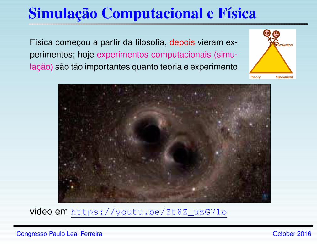
Simulação Computacional e Física
Física começou a partir da filosofia, depois vieram ex-
perimentos; hoje experimentos computacionais (simu-
lação) são tão importantes quanto teoria e experimento
video em https://youtu.be/Zt8Z_uzG71o
Congresso Paulo Leal Ferreira October 2016
Modelagem e Simulação
A simulação é um processo de projetar um modelo
computacional de um sistema real e conduzir experimentos
com este modelo com o propósito de entender seu
comportamento e/ou avaliar estratégias para sua operação.
D. Pegden (1990)
Congresso Paulo Leal Ferreira October 2016
Modelagem e Simulação
A simulação é um processo de projetar um modelo
computacional de um sistema real e conduzir experimentos
com este modelo com o propósito de entender seu
comportamento e/ou avaliar estratégias para sua operação.
D. Pegden (1990)
• simulação como teste e planejamento (e.g. gerenciamento
de empresas) em substituição a experimentos
• reconstrução para melhor compreensão de eventos
ocorridos (e.g. acidentes)
• modelagem de sistemas (e.g. bactérias)
Congresso Paulo Leal Ferreira October 2016
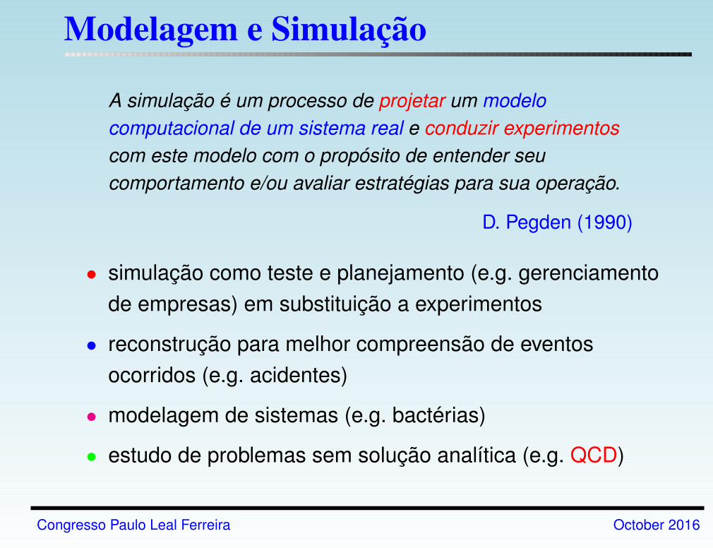
Modelagem e Simulação
A simulação é um processo de projetar um modelo
computacional de um sistema real e conduzir experimentos
com este modelo com o propósito de entender seu
comportamento e/ou avaliar estratégias para sua operação.
D. Pegden (1990)
• simulação como teste e planejamento (e.g. gerenciamento
de empresas) em substituição a experimentos
• reconstrução para melhor compreensão de eventos
ocorridos (e.g. acidentes)
• modelagem de sistemas (e.g. bactérias)
• estudo de problemas sem solução analítica (e.g. QCD)
Congresso Paulo Leal Ferreira October 2016
Simulação Numérica de Monte Carlo
Método para simulação computacional (experimento virtual, teórico!)
Evolução temporal (dinâmica) do sistema no computador: dada pelas
leis físicas (equações diferenciais) ou modelo; pode ser estocástico
Note: Sistema parece evoluir por conta própria, realizamos medidas,
analisamos dados, mas... ainda é teoria!
aplicação: experimentos que não podemos/não queremos realizar
(projeto de aviões, guerra nuclear, evolução)
também: casos em que não há formulação física: Sistema fictício
⇒ modelagem (in silico) de sistemas biológicos (e.g. bactérias)
⇒ estudo de sistemas complexos
ou: sistema real, dinâmica fictícia (truque!)
⇒ estudo de problemas sem solução analítica (e.g. QCD)
Congresso Paulo Leal Ferreira October 2016
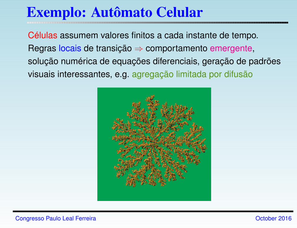
Exemplo: Autômato Celular
Células assumem valores finitos a cada instante de tempo.
Regras locais de transição ⇒ comportamento emergente,
solução numérica de equações diferenciais, geração de padrões
visuais interessantes, e.g. agregação limitada por difusão
Congresso Paulo Leal Ferreira October 2016
O Jogo da Vida
Autômatos determinísticos, com regras simples, ilustram o
comportamento de diversos sistemas físicos (e.g. autômatos
unidimensionais de Wolfram)
⇒ Jogo da Vida, proposto em 1970 por J. Conway, pode
modelar a dinâmica populacional de formas simples de vida
(e.g. colônias de bactérias).
Tabuleiro de células, com as regras:
células com menos de 2 ou mais de 3 vizinhos morrem
células com 2 ou 3 vizinhos vivos sobrevivem
indivíduos nascem em células vazias com 3 vizinhos
Congresso Paulo Leal Ferreira October 2016
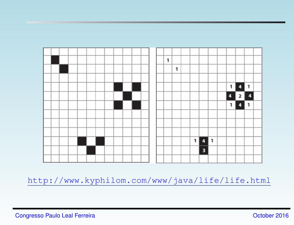
http://www.kyphilom.com/www/java/life/life.html
Congresso Paulo Leal Ferreira October 2016
Aplicações do Método de Monte Carlo
Mecânica Estatística: descrição de sistemas de muitos
corpos (≈ 1023 corpos...) utilizando grandezas médias
⇒ comportamento macroscópico (termodinâmica) a
partir da descrição microscópica de sistemas como
fluidos/gases, modelos de materiais magnéticos,
sistemas biológicos; tratamento de fenômenos críticos,
sistemas complexos.
Matéria Condensada: descrição aproximada de
sistemas quânticos, polímeros, fluidos complexos,
propriedades condutoras/magnéticas.
Congresso Paulo Leal Ferreira October 2016
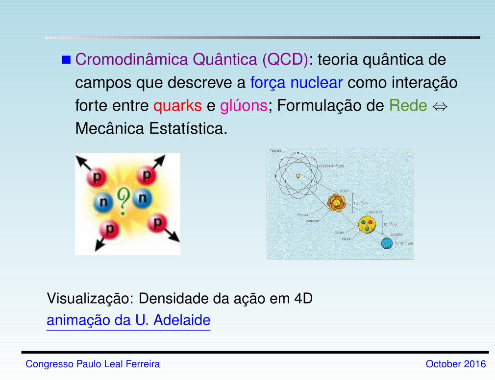
Cromodinâmica Quântica (QCD): teoria quântica de
campos que descreve a força nuclear como interação
forte entre quarks e glúons; Formulação de Rede ⇔Mecânica Estatística.
Visualização: Densidade da ação em 4D
animação da U. Adelaide
Congresso Paulo Leal Ferreira October 2016
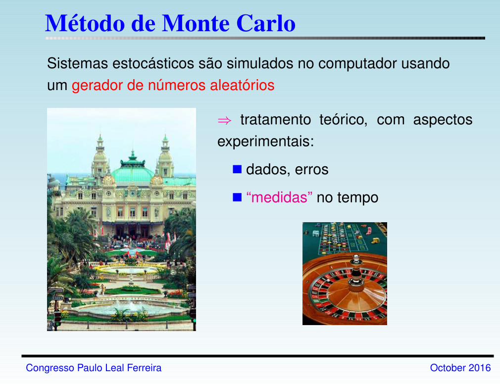
Método de Monte Carlo
Sistemas estocásticos são simulados no computador usando
um gerador de números aleatórios
⇒ tratamento teórico, com aspectos
experimentais:
dados, erros
“medidas” no tempo
Congresso Paulo Leal Ferreira October 2016

Gerador de Números Aleatórios
Anyone who considers arithmetical methods of
producing random digits is, of course, in a state of sin.
John Von Neumann (1951)
gerador = prescrição algébrica que produz sequência de
números ri com distribuição desejada (em geral uniforme
em [0,1]) dada uma semente.
Nota: esta sequência é determinística, a operação
repetida a partir do mesmo ponto inicial gera a mesma
sequência ⇒ números pseudo-aleatórios.
Congresso Paulo Leal Ferreira October 2016
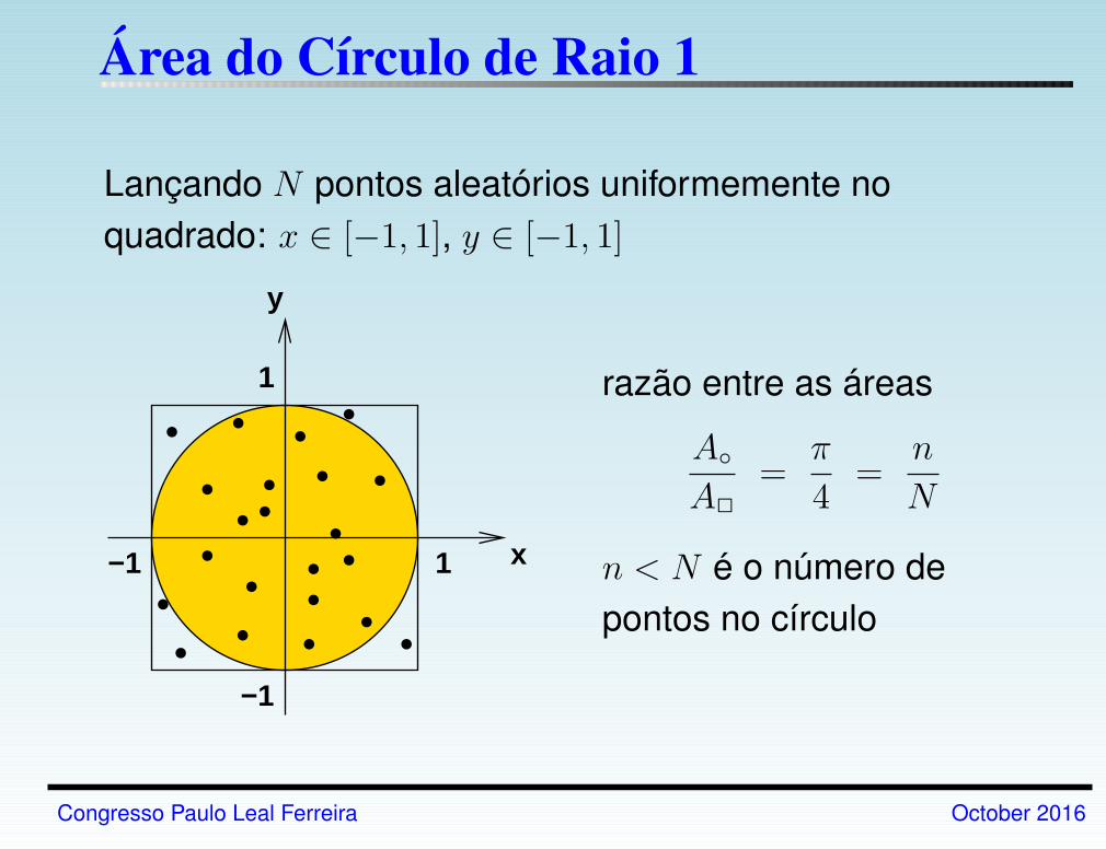
Área do Círculo de Raio 1
Lançando N pontos aleatórios uniformemente no
quadrado: x ∈ [−1, 1], y ∈ [−1, 1]
y
−1
−1
1
1
x.... .... .
..
.. ..
..
.
.
.
. .razão entre as áreas
A
A
=π
4=
n
N
n < N é o número de
pontos no círculo
Congresso Paulo Leal Ferreira October 2016
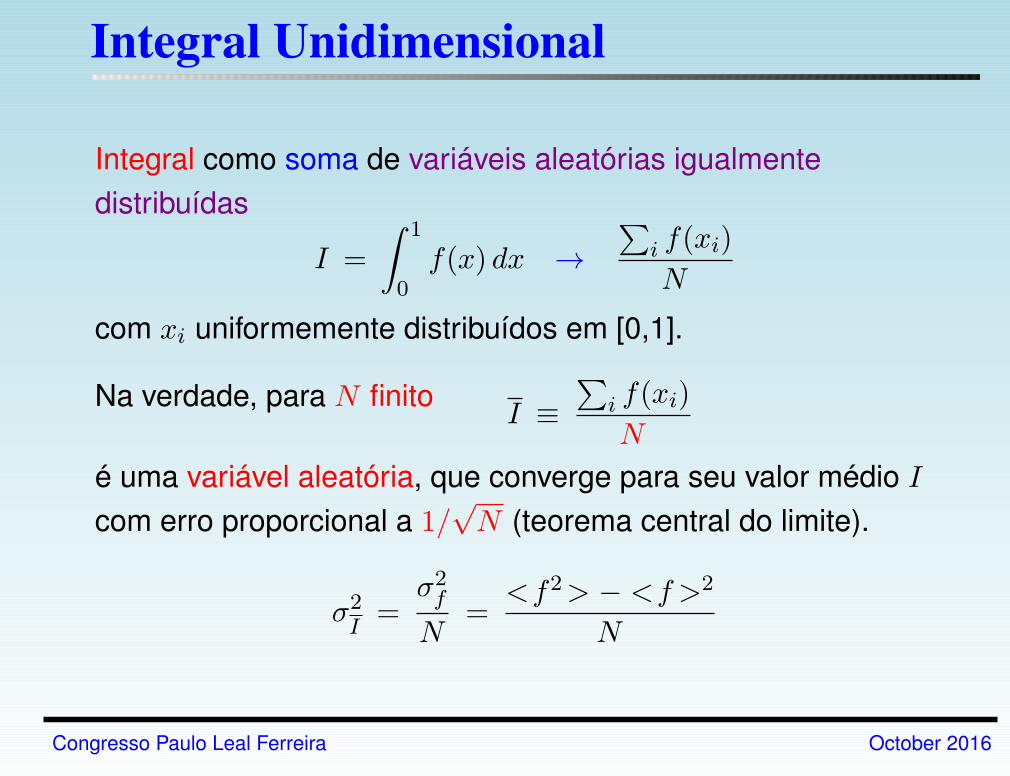
Integral Unidimensional
Integral como soma de variáveis aleatórias igualmente
distribuídas
I =
∫ 1
0f(x) dx →
∑i f(xi)
N
com xi uniformemente distribuídos em [0,1].
Na verdade, para N finitoI ≡
∑i f(xi)
N
é uma variável aleatória, que converge para seu valor médio I
com erro proporcional a 1/√N (teorema central do limite).
σ2I=
σ2fN
=<f2> − <f >2
N
Congresso Paulo Leal Ferreira October 2016
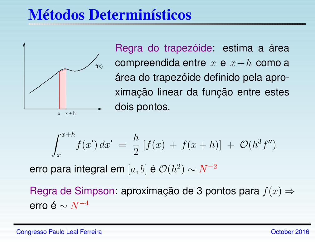
Métodos Determinísticos
f(x)
x x + h
Regra do trapezóide: estima a área
compreendida entre x e x+h como a
área do trapezóide definido pela apro-
ximação linear da função entre estes
dois pontos.
∫ x+h
x
f(x′) dx′ =h
2[f(x) + f(x+ h)] + O(h3f ′′)
erro para integral em [a, b] é O(h2) ∼ N−2
Regra de Simpson: aproximação de 3 pontos para f(x) ⇒erro é ∼ N−4
Congresso Paulo Leal Ferreira October 2016
Comparação
d = 1:
métodos determinísticos tipicamente têm erros
O(N−2) (regra do trapézio) ou ∼ O(N−4) (regra de
Simpson); Monte Carlo tem O(N−1/2): com 2N pontos
o erro diminui por um fator 4 (trapezóide), 16
(Simpson) ou√2 (Monte Carlo)
d > 1:
para integral d-dimensional N ∼ 1/hd ⇒ erro N−2/d
(trapezóide) ou N−4/d (Simpson) ⇒ Monte Carlo
começa a ser vantagem a partir de d = 8...
Congresso Paulo Leal Ferreira October 2016
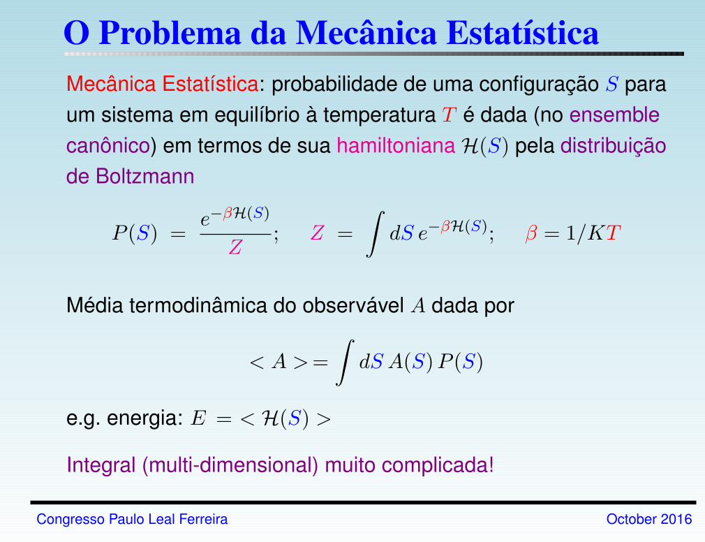
O Problema da Mecânica EstatísticaMecânica Estatística: probabilidade de uma configuração S para
um sistema em equilíbrio à temperatura T é dada (no ensemble
canônico) em termos de sua hamiltoniana H(S) pela distribuição
de Boltzmann
P (S) =e−βH(S)
Z; Z =
∫dS e−βH(S); β = 1/KT
Média termodinâmica do observável A dada por
< A >=
∫dS A(S)P (S)
e.g. energia: E = < H(S) >
Integral (multi-dimensional) muito complicada!
Congresso Paulo Leal Ferreira October 2016
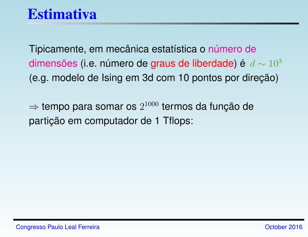
Estimativa
Tipicamente, em mecânica estatística o número de
dimensões (i.e. número de graus de liberdade) é d ∼ 103
(e.g. modelo de Ising em 3d com 10 pontos por direção)
⇒ tempo para somar os 21000 termos da função de
partição em computador de 1 Tflops:
Congresso Paulo Leal Ferreira October 2016
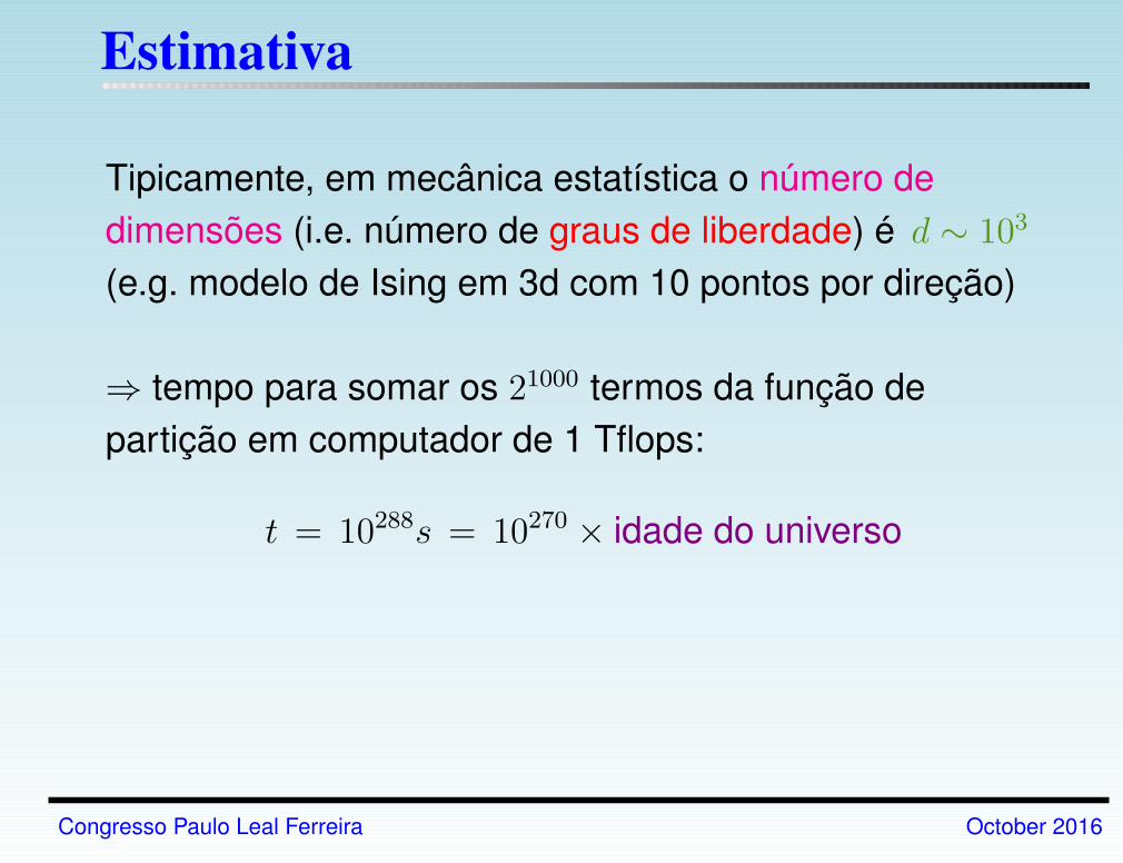
Estimativa
Tipicamente, em mecânica estatística o número de
dimensões (i.e. número de graus de liberdade) é d ∼ 103
(e.g. modelo de Ising em 3d com 10 pontos por direção)
⇒ tempo para somar os 21000 termos da função de
partição em computador de 1 Tflops:
t = 10288s = 10270 × idade do universo
Congresso Paulo Leal Ferreira October 2016
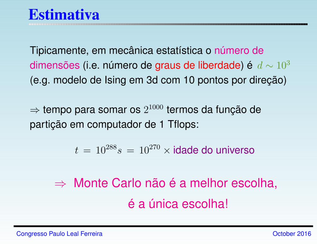
Estimativa
Tipicamente, em mecânica estatística o número de
dimensões (i.e. número de graus de liberdade) é d ∼ 103
(e.g. modelo de Ising em 3d com 10 pontos por direção)
⇒ tempo para somar os 21000 termos da função de
partição em computador de 1 Tflops:
t = 10288s = 10270 × idade do universo
⇒ Monte Carlo não é a melhor escolha,
é a única escolha!
Congresso Paulo Leal Ferreira October 2016
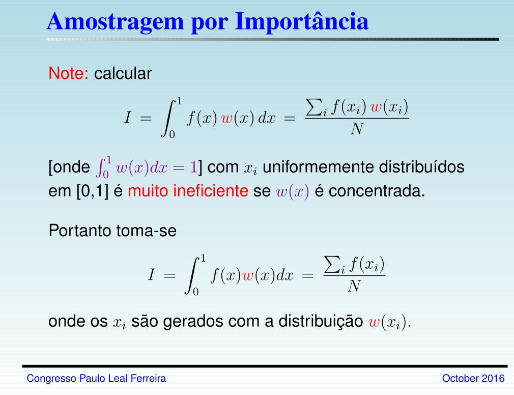
Amostragem por Importância
Note: calcular
I =
∫ 1
0
f(x)w(x) dx =
∑i f(xi)w(xi)
N
[onde∫ 1
0w(x)dx = 1] com xi uniformemente distribuídos
em [0,1] é muito ineficiente se w(x) é concentrada.
Portanto toma-se
I =
∫ 1
0
f(x)w(x)dx =
∑i f(xi)
N
onde os xi são gerados com a distribuição w(xi).
Congresso Paulo Leal Ferreira October 2016
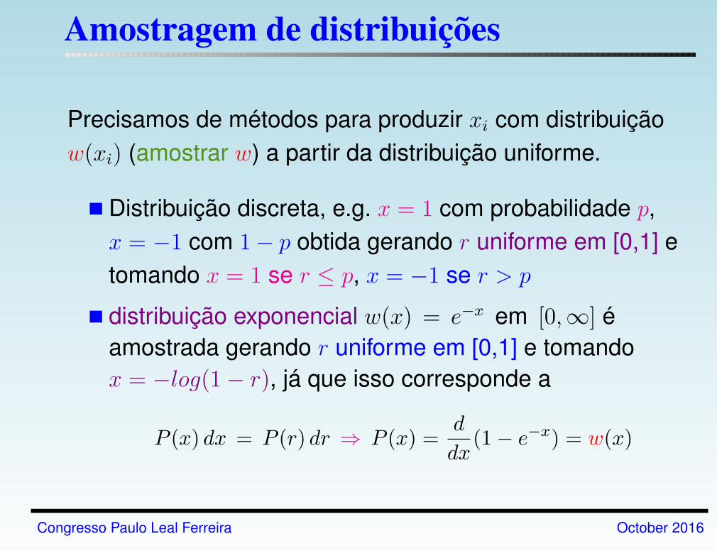
Amostragem de distribuições
Precisamos de métodos para produzir xi com distribuição
w(xi) (amostrar w) a partir da distribuição uniforme.
Distribuição discreta, e.g. x = 1 com probabilidade p,
x = −1 com 1− p obtida gerando r uniforme em [0,1] e
tomando x = 1 se r ≤ p, x = −1 se r > p
distribuição exponencial w(x) = e−x em [0,∞] é
amostrada gerando r uniforme em [0,1] e tomando
x = −log(1− r), já que isso corresponde a
P (x) dx = P (r) dr ⇒ P (x) =d
dx(1− e−x) = w(x)
Congresso Paulo Leal Ferreira October 2016
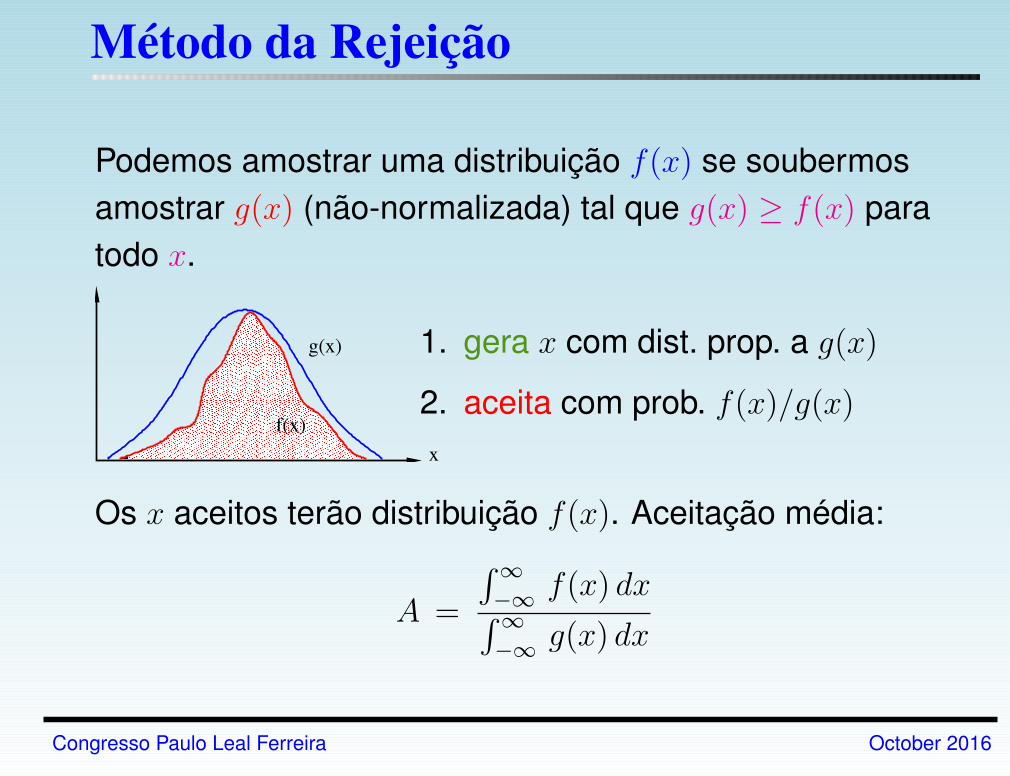
Método da Rejeição
Podemos amostrar uma distribuição f(x) se soubermos
amostrar g(x) (não-normalizada) tal que g(x) ≥ f(x) para
todo x.
1. gera x com dist. prop. a g(x)
2. aceita com prob. f(x)/g(x)
Os x aceitos terão distribuição f(x). Aceitação média:
A =
∫∞
−∞f(x) dx∫∞
−∞g(x) dx
Congresso Paulo Leal Ferreira October 2016
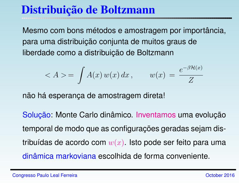
Distribuição de Boltzmann
Mesmo com bons métodos e amostragem por importância,
para uma distribuição conjunta de muitos graus de
liberdade como a distribuição de Boltzmann
< A >=
∫A(x)w(x) dx , w(x) =
e−βH(x)
Z
não há esperança de amostragem direta!
Solução: Monte Carlo dinâmico. Inventamos uma evolução
temporal de modo que as configurações geradas sejam dis-
tribuídas de acordo com w(x). Isto pode ser feito para uma
dinâmica markoviana escolhida de forma conveniente.
Congresso Paulo Leal Ferreira October 2016
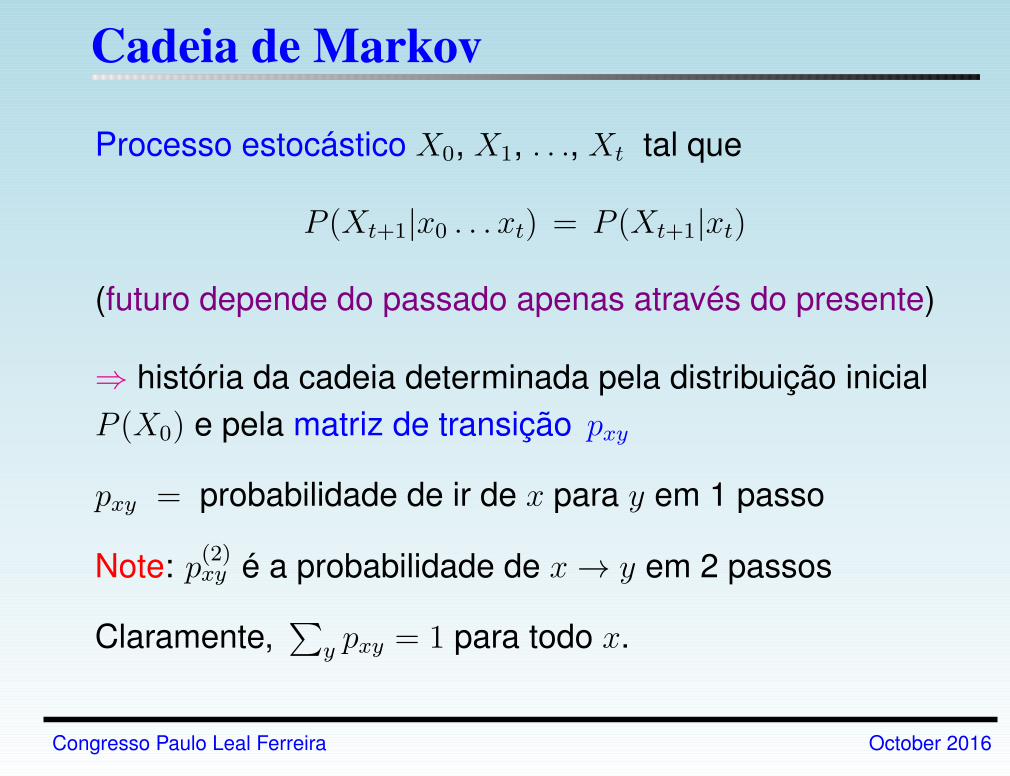
Cadeia de Markov
Processo estocástico X0, X1, . . ., Xt tal que
P (Xt+1|x0 . . . xt) = P (Xt+1|xt)
(futuro depende do passado apenas através do presente)
⇒ história da cadeia determinada pela distribuição inicial
P (X0) e pela matriz de transição pxy
pxy = probabilidade de ir de x para y em 1 passo
Note: p(2)xy é a probabilidade de x → y em 2 passos
Claramente,∑
y pxy = 1 para todo x.
Congresso Paulo Leal Ferreira October 2016
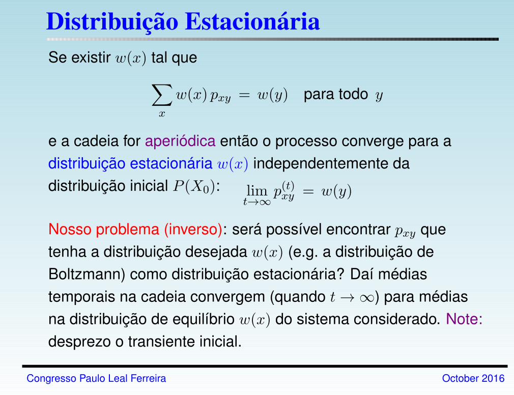
Distribuição EstacionáriaSe existir w(x) tal que
∑
x
w(x) pxy = w(y) para todo y
e a cadeia for aperiódica então o processo converge para a
distribuição estacionária w(x) independentemente da
distribuição inicial P (X0): limt→∞
p(t)xy = w(y)
Nosso problema (inverso): será possível encontrar pxy que
tenha a distribuição desejada w(x) (e.g. a distribuição de
Boltzmann) como distribuição estacionária? Daí médias
temporais na cadeia convergem (quando t→ ∞) para médias
na distribuição de equilíbrio w(x) do sistema considerado. Note:
desprezo o transiente inicial.
Congresso Paulo Leal Ferreira October 2016
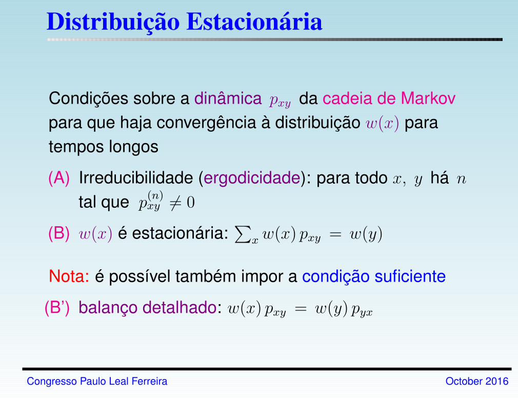
Distribuição Estacionária
Condições sobre a dinâmica pxy da cadeia de Markov
para que haja convergência à distribuição w(x) para
tempos longos
(A) Irreducibilidade (ergodicidade): para todo x, y há n
tal que p(n)xy 6= 0
(B) w(x) é estacionária:∑
x w(x) pxy = w(y)
Nota: é possível também impor a condição suficiente
(B’) balanço detalhado: w(x) pxy = w(y) pyx
Congresso Paulo Leal Ferreira October 2016
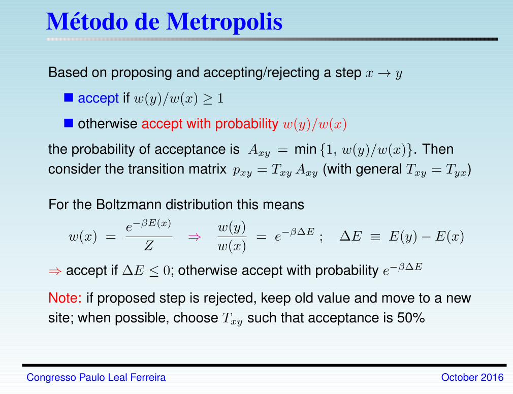
Método de Metropolis
Based on proposing and accepting/rejecting a step x→ y
accept if w(y)/w(x) ≥ 1
otherwise accept with probability w(y)/w(x)
the probability of acceptance is Axy = min 1, w(y)/w(x). Then
consider the transition matrix pxy = Txy Axy (with general Txy = Tyx)
For the Boltzmann distribution this means
w(x) =e−βE(x)
Z⇒ w(y)
w(x)= e−β∆E ; ∆E ≡ E(y)− E(x)
⇒ accept if ∆E ≤ 0; otherwise accept with probability e−β∆E
Note: if proposed step is rejected, keep old value and move to a new
site; when possible, choose Txy such that acceptance is 50%
Congresso Paulo Leal Ferreira October 2016
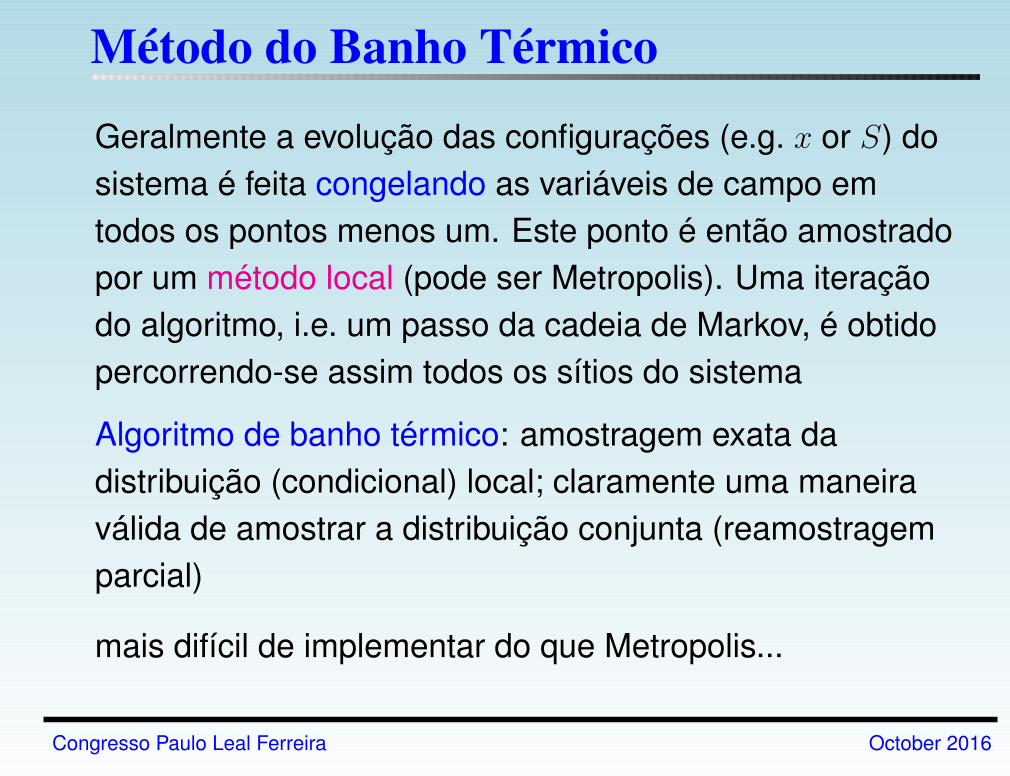
Método do Banho Térmico
Geralmente a evolução das configurações (e.g. x or S) do
sistema é feita congelando as variáveis de campo em
todos os pontos menos um. Este ponto é então amostrado
por um método local (pode ser Metropolis). Uma iteração
do algoritmo, i.e. um passo da cadeia de Markov, é obtido
percorrendo-se assim todos os sítios do sistema
Algoritmo de banho térmico: amostragem exata da
distribuição (condicional) local; claramente uma maneira
válida de amostrar a distribuição conjunta (reamostragem
parcial)
mais difícil de implementar do que Metropolis...
Congresso Paulo Leal Ferreira October 2016
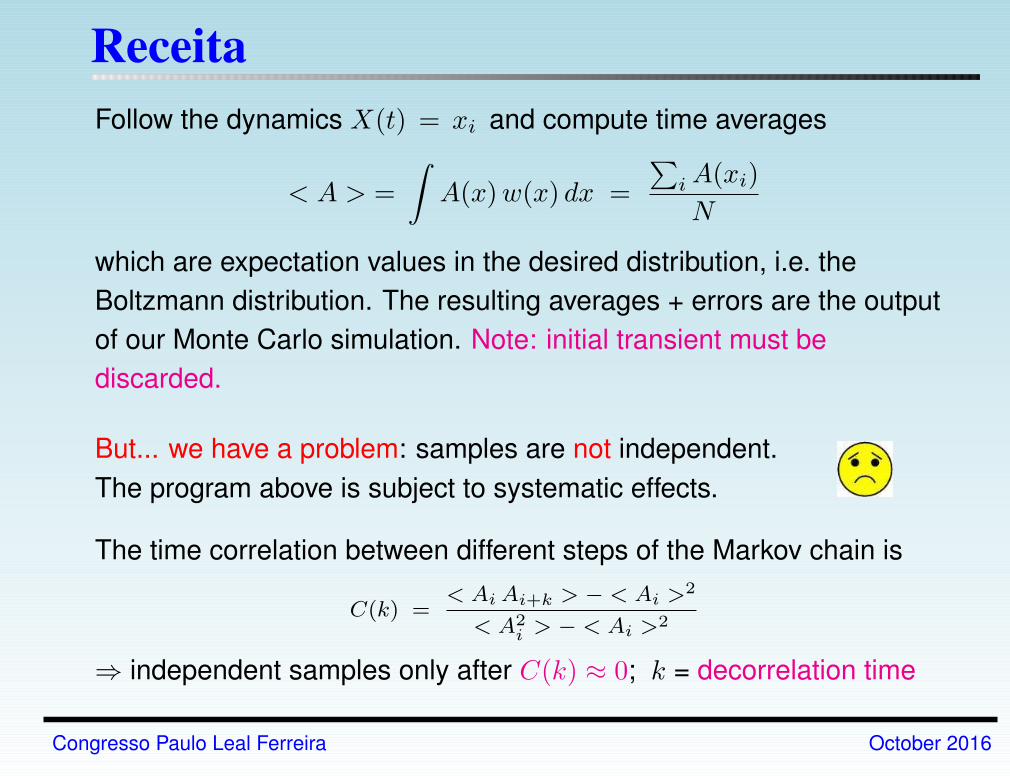
ReceitaFollow the dynamics X(t) = xi and compute time averages
< A > =
∫A(x)w(x) dx =
∑iA(xi)
N
which are expectation values in the desired distribution, i.e. the
Boltzmann distribution. The resulting averages + errors are the output
of our Monte Carlo simulation. Note: initial transient must be
discarded.
But... we have a problem: samples are not independent.
The program above is subject to systematic effects.
The time correlation between different steps of the Markov chain is
C(k) =< Ai Ai+k > − < Ai >
2
< A2i > − < Ai >2
⇒ independent samples only after C(k) ≈ 0; k = decorrelation time
Congresso Paulo Leal Ferreira October 2016
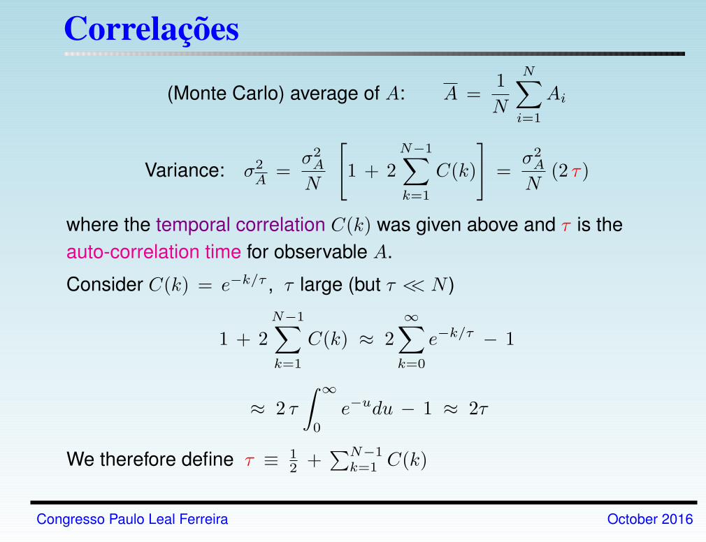
Correlações
(Monte Carlo) average of A: A =1
N
N∑
i=1
Ai
Variance: σ2A
=σ2A
N
[1 + 2
N−1∑
k=1
C(k)
]=
σ2A
N(2 τ)
where the temporal correlation C(k) was given above and τ is the
auto-correlation time for observable A.
Consider C(k) = e−k/τ , τ large (but τ << N )
1 + 2
N−1∑
k=1
C(k) ≈ 2
∞∑
k=0
e−k/τ − 1
≈ 2 τ
∫ ∞
0
e−udu − 1 ≈ 2τ
We therefore define τ ≡ 12 +
∑N−1k=1 C(k)
Congresso Paulo Leal Ferreira October 2016
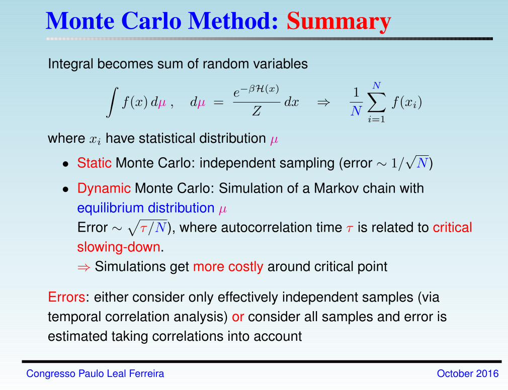
Monte Carlo Method: Summary
Integral becomes sum of random variables
∫f(x) dµ , dµ =
e−βH(x)
Zdx ⇒ 1
N
N∑
i=1
f(xi)
where xi have statistical distribution µ
• Static Monte Carlo: independent sampling (error ∼ 1/√N )
• Dynamic Monte Carlo: Simulation of a Markov chain with
equilibrium distribution µ
Error ∼√τ/N ), where autocorrelation time τ is related to critical
slowing-down.
⇒ Simulations get more costly around critical point
Errors: either consider only effectively independent samples (via
temporal correlation analysis) or consider all samples and error is
estimated taking correlations into account
Congresso Paulo Leal Ferreira October 2016
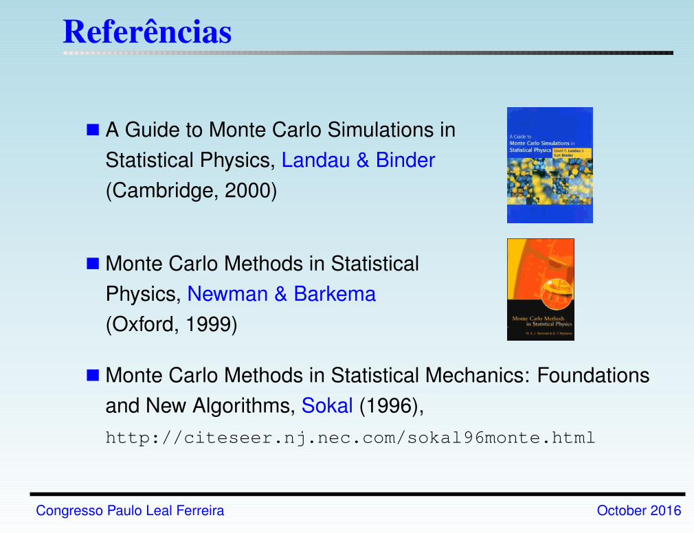
Referências
A Guide to Monte Carlo Simulations in
Statistical Physics, Landau & Binder
(Cambridge, 2000)
Monte Carlo Methods in Statistical
Physics, Newman & Barkema
(Oxford, 1999)
Monte Carlo Methods in Statistical Mechanics: Foundations
and New Algorithms, Sokal (1996),
http://citeseer.nj.nec.com/sokal96monte.html
Congresso Paulo Leal Ferreira October 2016
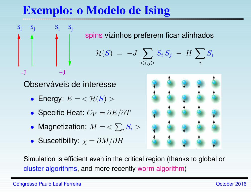
Exemplo: o Modelo de IsingS Si j
-J +J
S Si j
spins vizinhos preferem ficar alinhados
H(S) = −J∑
<i,j>
Si Sj − H∑
i
Si
Observáveis de interesse
• Energy: E =< H(S) >
• Specific Heat: CV = ∂E/∂T
• Magnetization: M =<∑
i Si >
• Suscetibility: χ = ∂M/∂H
Simulation is efficient even in the critical region (thanks to global or
cluster algorithms, and more recently worm algorithm)
Congresso Paulo Leal Ferreira October 2016
Example: Color confinement
Why are there no free color charged particles (quarks or gluons), but
only objects built out of them (hadrons), like mesons and baryons?
How does this phenomenon emerge from QCD?
Congresso Paulo Leal Ferreira October 2016
Example: Color confinement
Why are there no free color charged particles (quarks or gluons), but
only objects built out of them (hadrons), like mesons and baryons?
How does this phenomenon emerge from QCD?
⇒ Color confinement is a long withstanding theoretical problem within
the Standard Model
Congresso Paulo Leal Ferreira October 2016
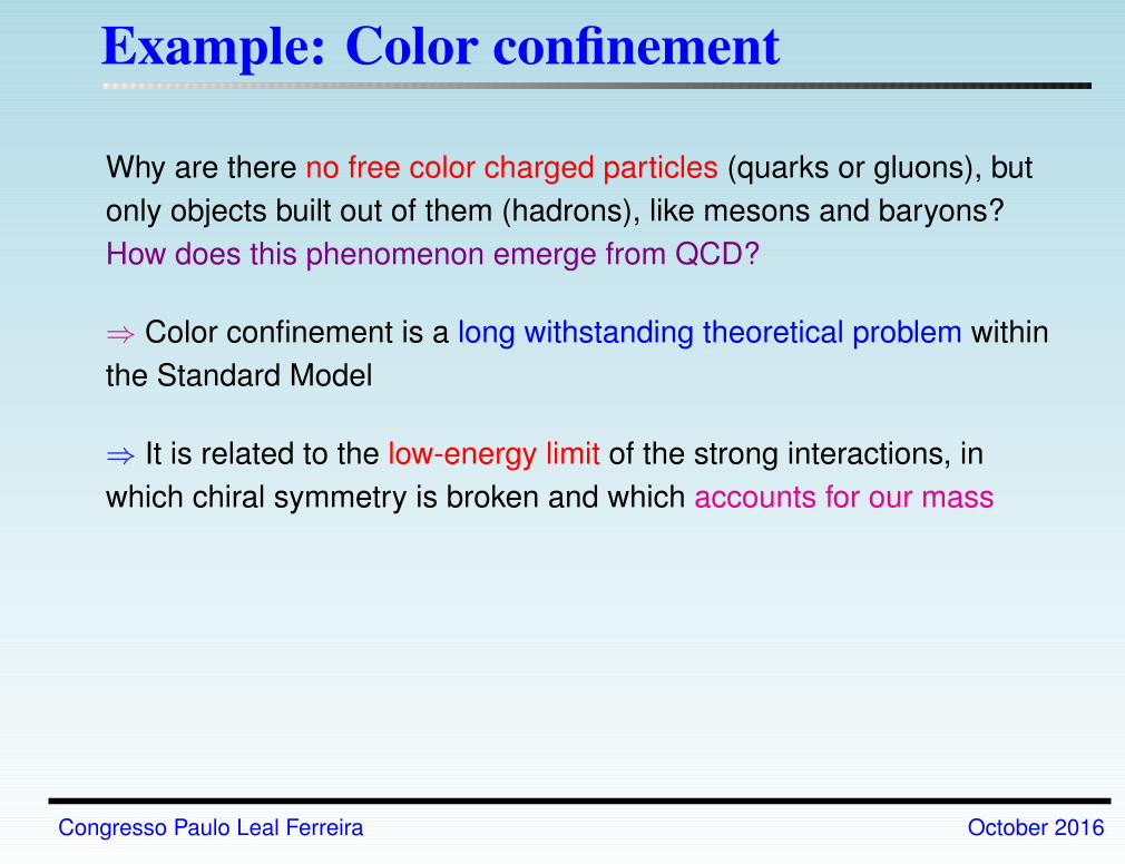
Example: Color confinement
Why are there no free color charged particles (quarks or gluons), but
only objects built out of them (hadrons), like mesons and baryons?
How does this phenomenon emerge from QCD?
⇒ Color confinement is a long withstanding theoretical problem within
the Standard Model
⇒ It is related to the low-energy limit of the strong interactions, in
which chiral symmetry is broken and which accounts for our mass
Congresso Paulo Leal Ferreira October 2016
Example: Color confinement
Why are there no free color charged particles (quarks or gluons), but
only objects built out of them (hadrons), like mesons and baryons?
How does this phenomenon emerge from QCD?
⇒ Color confinement is a long withstanding theoretical problem within
the Standard Model
⇒ It is related to the low-energy limit of the strong interactions, in
which chiral symmetry is broken and which accounts for our mass
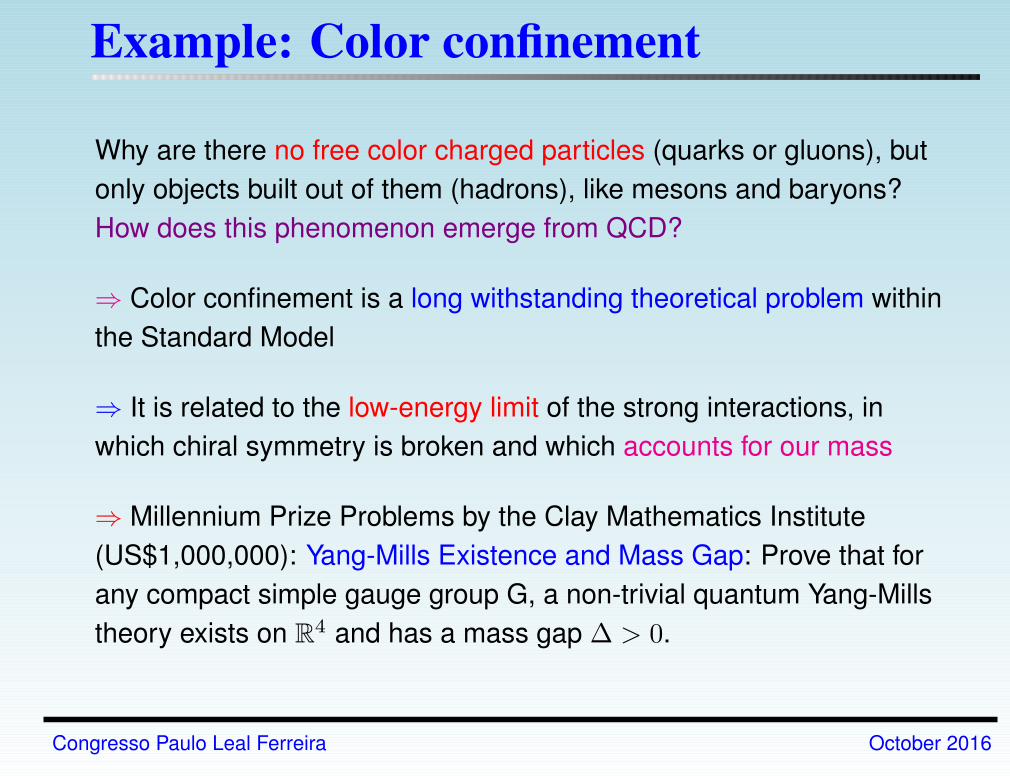
⇒ Millennium Prize Problems by the Clay Mathematics Institute
(US$1,000,000): Yang-Mills Existence and Mass Gap: Prove that for
any compact simple gauge group G, a non-trivial quantum Yang-Mills
theory exists on R4 and has a mass gap ∆ > 0.
Congresso Paulo Leal Ferreira October 2016
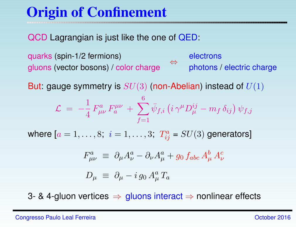
Origin of Confinement
QCD Lagrangian is just like the one of QED:
quarks (spin-1/2 fermions)
gluons (vector bosons) / color charge⇔ electrons
photons / electric charge
But: gauge symmetry is SU(3) (non-Abelian) instead of U(1)
L = −1
4F aµν F
µνa +
6∑
f=1
ψf,i
(i γµDij
µ −mf δij)ψf,j
where [a = 1, . . . , 8; i = 1, . . . , 3; T aij = SU(3) generators]
F aµν ≡ ∂µA
aν − ∂νA
aµ + g0 fabcA
bµA
cν
Dµ ≡ ∂µ − i g0Aaµ Ta
3- & 4-gluon vertices ⇒ gluons interact ⇒ nonlinear effects
Congresso Paulo Leal Ferreira October 2016
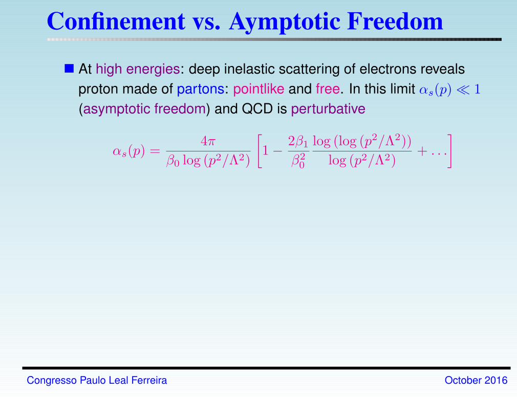
Confinement vs. Aymptotic Freedom
At high energies: deep inelastic scattering of electrons reveals
proton made of partons: pointlike and free. In this limit αs(p) ≪ 1
(asymptotic freedom) and QCD is perturbative
αs(p) =4π
β0 log (p2/Λ2)
[1− 2β1
β20
log (log (p2/Λ2))
log (p2/Λ2)+ . . .
]
Congresso Paulo Leal Ferreira October 2016
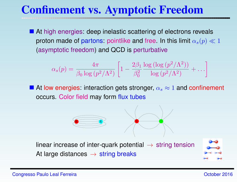
Confinement vs. Aymptotic Freedom
At high energies: deep inelastic scattering of electrons reveals
proton made of partons: pointlike and free. In this limit αs(p) ≪ 1
(asymptotic freedom) and QCD is perturbative
αs(p) =4π
β0 log (p2/Λ2)
[1− 2β1
β20
log (log (p2/Λ2))
log (p2/Λ2)+ . . .
]
At low energies: interaction gets stronger, αs ≈ 1 and confinement
occurs. Color field may form flux tubes
q− −q +
linear increase of inter-quark potential → string tension
At large distances → string breaks
Congresso Paulo Leal Ferreira October 2016
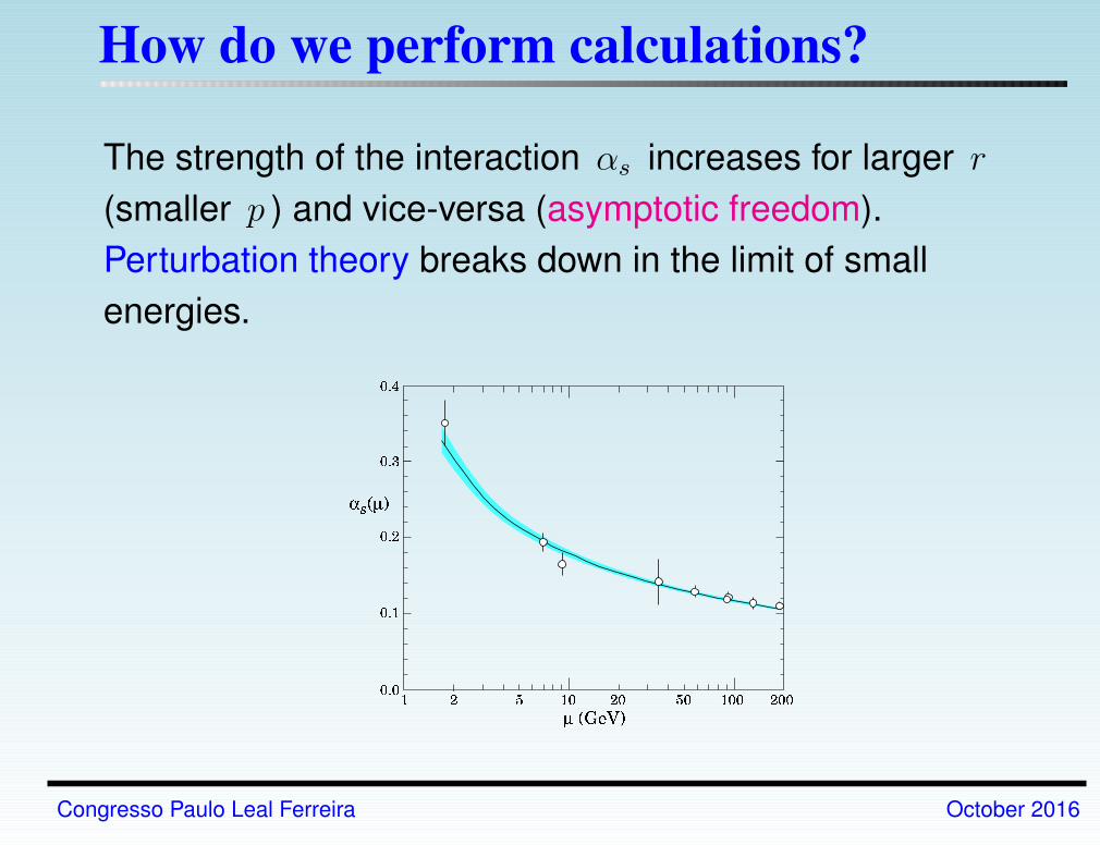
How do we perform calculations?
The strength of the interaction αs increases for larger r
(smaller p ) and vice-versa (asymptotic freedom).
Perturbation theory breaks down in the limit of small
energies.
Congresso Paulo Leal Ferreira October 2016
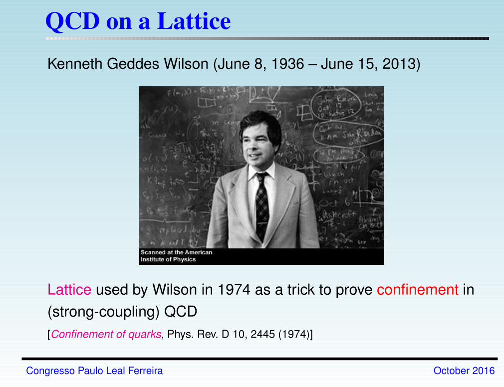
QCD on a Lattice
Kenneth Geddes Wilson (June 8, 1936 – June 15, 2013)
Lattice used by Wilson in 1974 as a trick to prove confinement in
(strong-coupling) QCD
[Confinement of quarks, Phys. Rev. D 10, 2445 (1974)]
Congresso Paulo Leal Ferreira October 2016
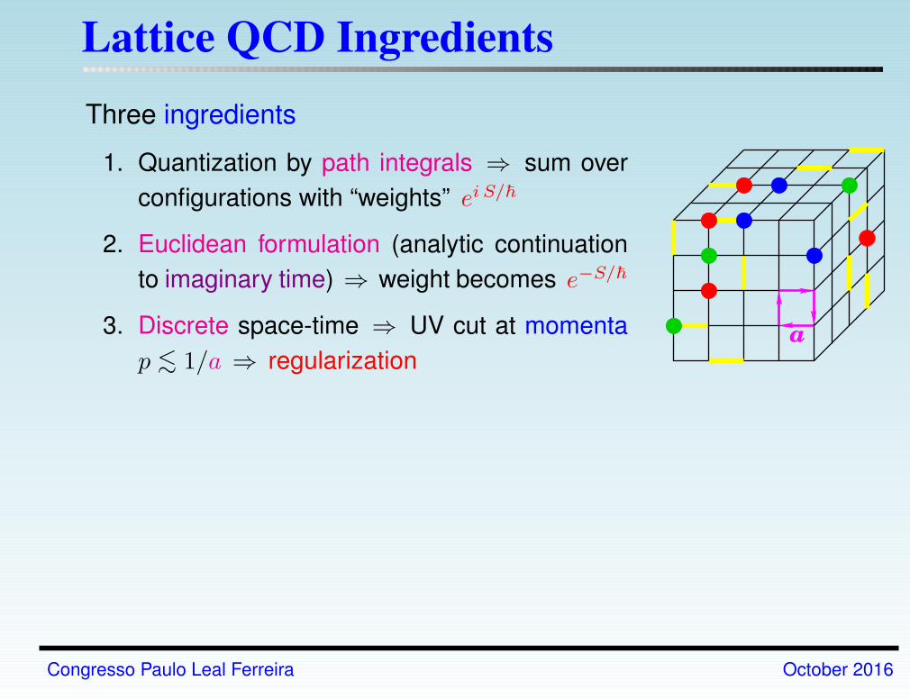
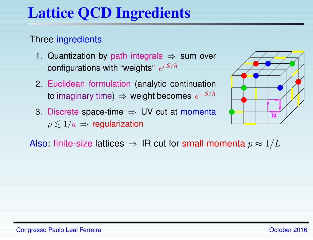
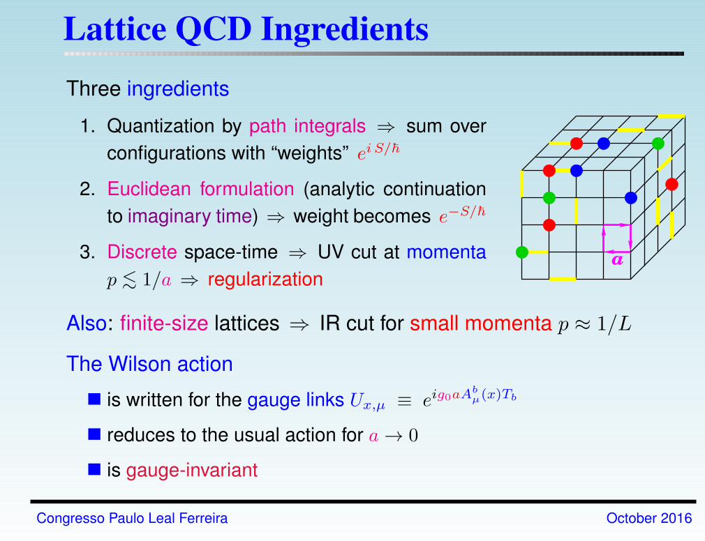
Lattice QCD Ingredients
Three ingredients
1. Quantization by path integrals ⇒ sum over
configurations with “weights” ei S/~
2. Euclidean formulation (analytic continuation
to imaginary time) ⇒ weight becomes e−S/~
3. Discrete space-time ⇒ UV cut at momenta
p ∼< 1/a ⇒ regularization
Congresso Paulo Leal Ferreira October 2016
Lattice QCD Ingredients
Three ingredients
1. Quantization by path integrals ⇒ sum over
configurations with “weights” ei S/~
2. Euclidean formulation (analytic continuation
to imaginary time) ⇒ weight becomes e−S/~
3. Discrete space-time ⇒ UV cut at momenta
p ∼< 1/a ⇒ regularization
Also: finite-size lattices ⇒ IR cut for small momenta p ≈ 1/L
The Wilson action
is written for the gauge links Ux,µ ≡ eig0aAbµ(x)Tb
reduces to the usual action for a→ 0
is gauge-invariant
Congresso Paulo Leal Ferreira October 2016
The Lattice Action
The Wilson action (1974)
S = −β3
∑
ReTrU , Ux,µ ≡ eig0aAbµ(x)Tb , β = 6/g0
2
written in terms of oriented plaquettes formed by the link variables
Ux,µ, which are group elements
under gauge transformations: Ux,µ → g(x)Ux,µ g†(x+ µ), where
g ∈ SU(3) ⇒ closed loops are gauge-invariant quantities
integration volume is finite: no need for gauge-fixing
At small β (i.e. strong coupling) we can perform an expansion
analogous to the high-temperature expansion in statistical mechanics.
At lowest order, the only surviving terms are represented by diagrams
with “double” or “partner” links, i.e. the same link should appear in both
orientations, since∫dU Ux,µ = 0
Congresso Paulo Leal Ferreira October 2016
Confinement and Area Law
Considering a rectangular loop with sides R and T (the Wilson loop) as
our observable, the leading contribution to the observable’s
expectation value is obtained by “tiling” its inside with plaquettes,
yielding the area law
< W (R, T ) > ∼ βRT
But this observable is related to the interquark potential for a static
quark-antiquark pair
< W (R, T ) > = e−V (R)T
We thus have V (R) ∼ σR, demonstrating confinement at strong
coupling (small β)!
Problem: the physical limit is at large β...
Congresso Paulo Leal Ferreira October 2016
(Numerical) Lattice QCD
Classical Statistical-Mechanics model with the partition function
Z =
∫DU e−Sg
∫DψDψ e−
∫d4x ψ(x)K ψ(x) =
∫DU e−Sg detK(U)
Congresso Paulo Leal Ferreira October 2016

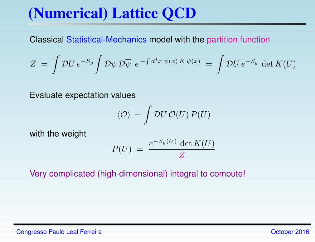
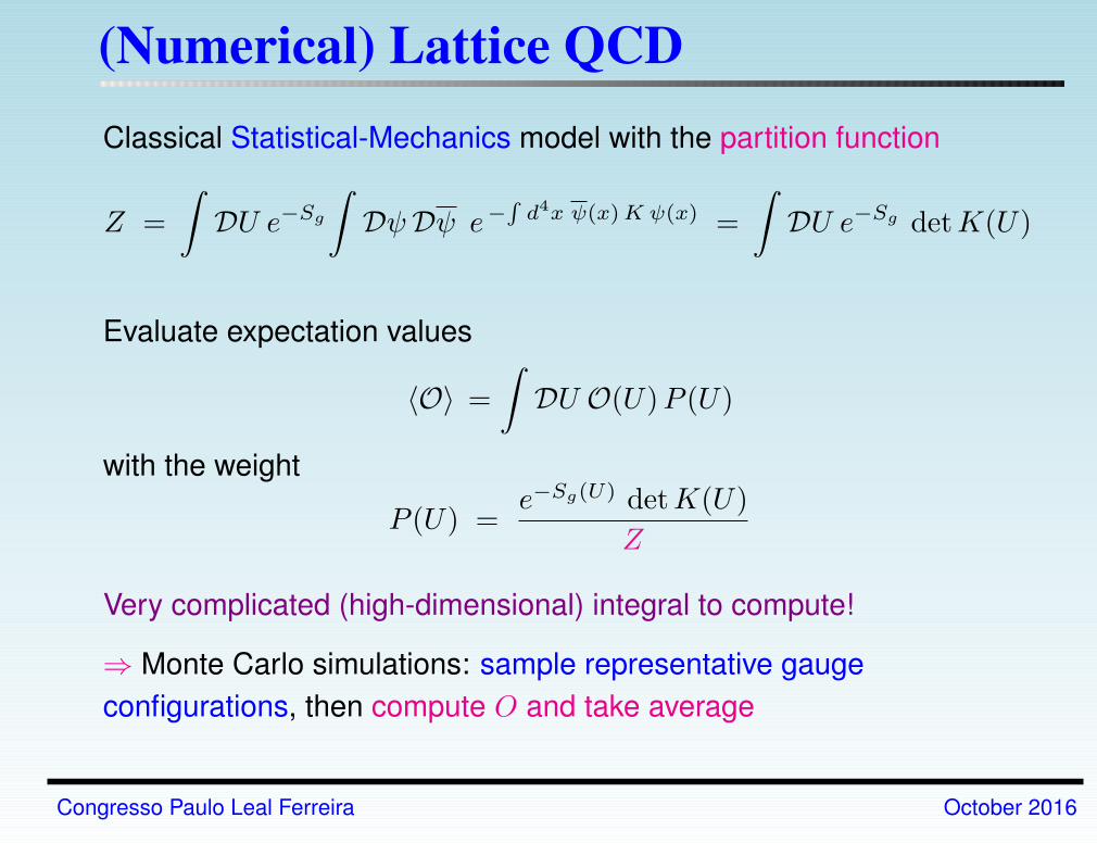
(Numerical) Lattice QCD
Classical Statistical-Mechanics model with the partition function
Z =
∫DU e−Sg
∫DψDψ e−
∫d4x ψ(x)K ψ(x) =
∫DU e−Sg detK(U)
Evaluate expectation values
〈O〉 =
∫DU O(U)P (U)
with the weight
P (U) =e−Sg(U) detK(U)
Z
Congresso Paulo Leal Ferreira October 2016
(Numerical) Lattice QCD
Classical Statistical-Mechanics model with the partition function
Z =
∫DU e−Sg
∫DψDψ e−
∫d4x ψ(x)K ψ(x) =
∫DU e−Sg detK(U)
Evaluate expectation values
〈O〉 =
∫DU O(U)P (U)
with the weight
P (U) =e−Sg(U) detK(U)
Z
Very complicated (high-dimensional) integral to compute!
⇒ Monte Carlo simulations: sample representative gauge
configurations, then compute O and take average
Congresso Paulo Leal Ferreira October 2016
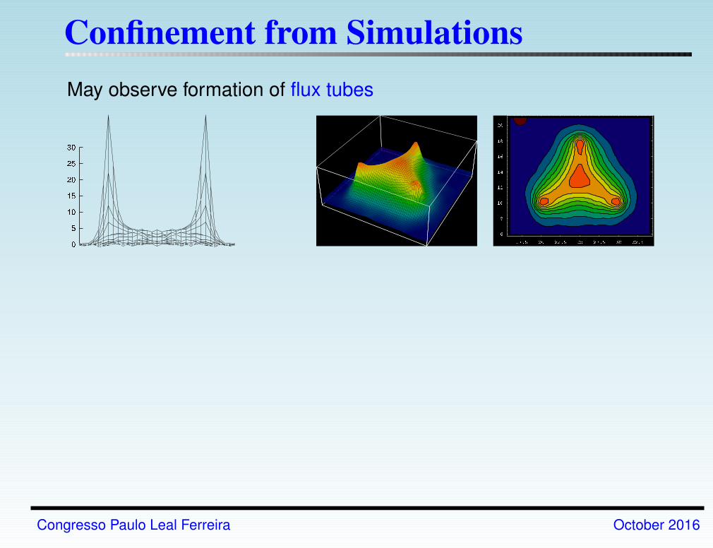
Confinement from Simulations
May observe formation of flux tubes
Congresso Paulo Leal Ferreira October 2016
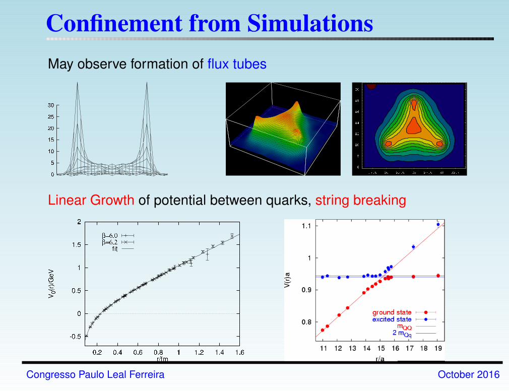
Confinement from Simulations
May observe formation of flux tubes
Linear Growth of potential between quarks, string breaking
Congresso Paulo Leal Ferreira October 2016
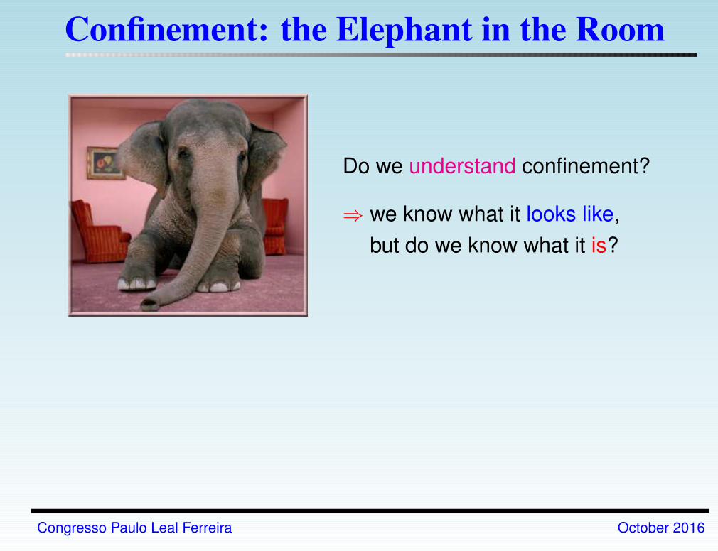
Confinement: the Elephant in the Room
Do we understand confinement?
⇒ we know what it looks like,
but do we know what it is?
Congresso Paulo Leal Ferreira October 2016
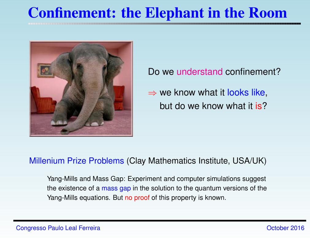
Confinement: the Elephant in the Room
Do we understand confinement?
⇒ we know what it looks like,
but do we know what it is?
Millenium Prize Problems (Clay Mathematics Institute, USA/UK)
Yang-Mills and Mass Gap: Experiment and computer simulations suggest
the existence of a mass gap in the solution to the quantum versions of the
Yang-Mills equations. But no proof of this property is known.
Congresso Paulo Leal Ferreira October 2016
Thoughts...
Today almost no one seriously doubts that quantum chromodynamics
confines quarks. Following many theoretical suggestions in the late 1970’s
about how quark confinement might come about, it was finally the computer
simulations of QCD, initiated by Creutz in 1980, that persuaded most
skeptics.
Quark confinement is now an old and familiar idea, routinely incorporated
into the standard model and all its proposed extensions, and the focus of
particle phenomenology shifted long ago to other issues.
But familiarity is not the same thing as understanding.
Despite efforts stretching over thirty years, there exists no derivation of quark
confinement starting from first principles, nor is there a totally convincing
explanation of the effect. It is fair to say that no theory of quark confinement
is generally accepted, and every proposal remains controversial.
J. Greensite (2003)
Congresso Paulo Leal Ferreira October 2016
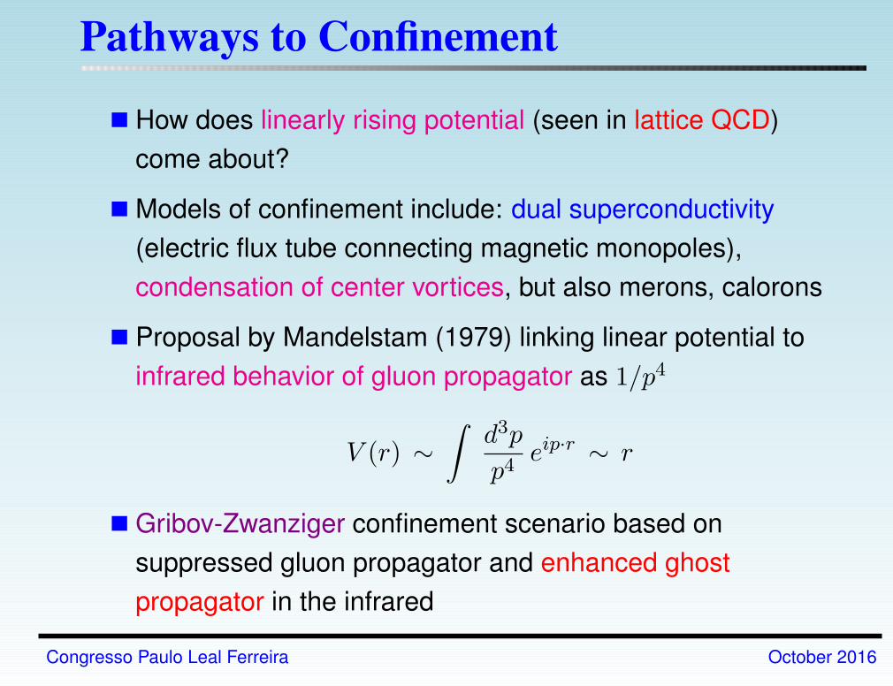
Pathways to Confinement
How does linearly rising potential (seen in lattice QCD)
come about?
Congresso Paulo Leal Ferreira October 2016
Pathways to Confinement
How does linearly rising potential (seen in lattice QCD)
come about?
Models of confinement include: dual superconductivity
(electric flux tube connecting magnetic monopoles),
condensation of center vortices, but also merons, calorons
Congresso Paulo Leal Ferreira October 2016
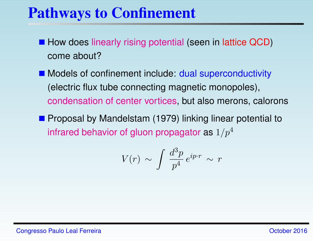
Pathways to Confinement
How does linearly rising potential (seen in lattice QCD)
come about?
Models of confinement include: dual superconductivity
(electric flux tube connecting magnetic monopoles),
condensation of center vortices, but also merons, calorons
Proposal by Mandelstam (1979) linking linear potential to
infrared behavior of gluon propagator as 1/p4
V (r) ∼∫
d3p
p4eip·r ∼ r
Congresso Paulo Leal Ferreira October 2016
Pathways to Confinement
How does linearly rising potential (seen in lattice QCD)
come about?
Models of confinement include: dual superconductivity
(electric flux tube connecting magnetic monopoles),
condensation of center vortices, but also merons, calorons
Proposal by Mandelstam (1979) linking linear potential to
infrared behavior of gluon propagator as 1/p4
V (r) ∼∫
d3p
p4eip·r ∼ r
Gribov-Zwanziger confinement scenario based on
suppressed gluon propagator and enhanced ghost
propagator in the infrared
Congresso Paulo Leal Ferreira October 2016
Ghost Propagator
Ghost fields are introduced as one evaluates functional integrals
by the Faddeev-Popov method, which restricts the space of
configurations through a gauge-fixing condition. The ghosts are
unphysical particles, since they correspond to anti-commuting
fields with spin zero.
Congresso Paulo Leal Ferreira October 2016
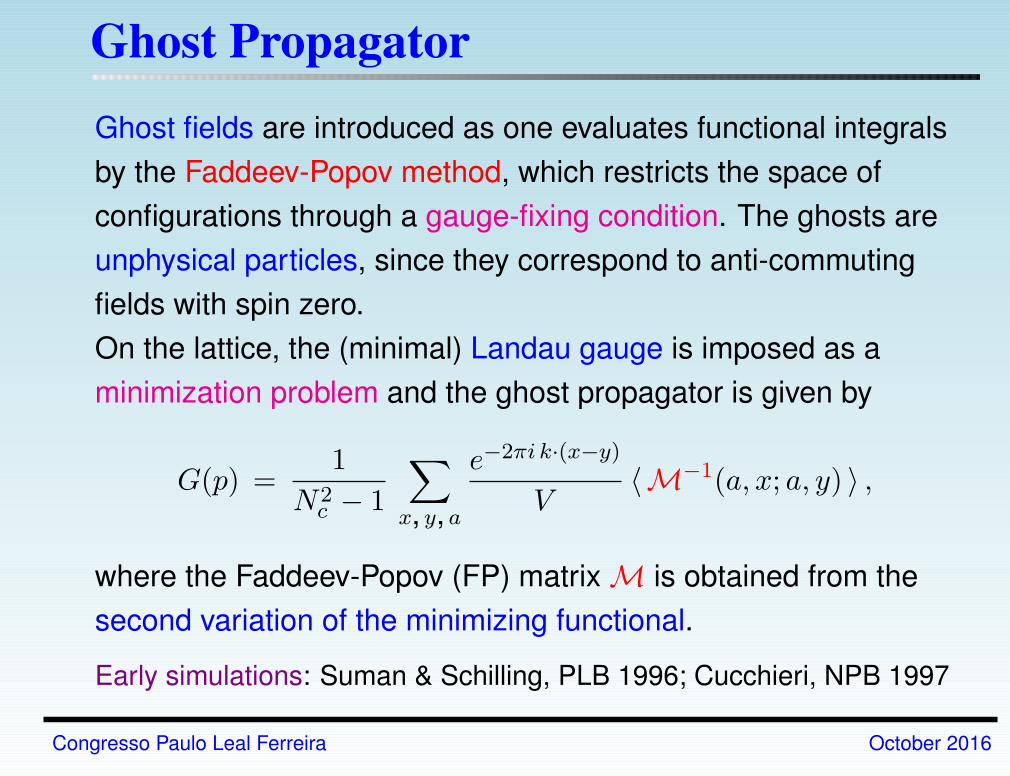
Ghost Propagator
Ghost fields are introduced as one evaluates functional integrals
by the Faddeev-Popov method, which restricts the space of
configurations through a gauge-fixing condition. The ghosts are
unphysical particles, since they correspond to anti-commuting
fields with spin zero.
On the lattice, the (minimal) Landau gauge is imposed as a
minimization problem and the ghost propagator is given by
G(p) =1
N2c − 1
∑
x, y, a
e−2πi k·(x−y)
V〈M−1(a, x; a, y) 〉 ,
where the Faddeev-Popov (FP) matrix M is obtained from the
second variation of the minimizing functional.
Early simulations: Suman & Schilling, PLB 1996; Cucchieri, NPB 1997
Congresso Paulo Leal Ferreira October 2016
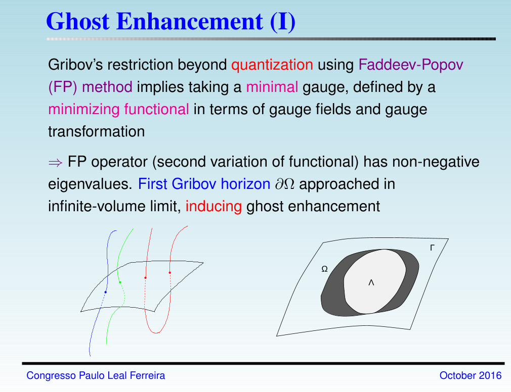
Ghost Enhancement (I)
Gribov’s restriction beyond quantization using Faddeev-Popov
(FP) method implies taking a minimal gauge, defined by a
minimizing functional in terms of gauge fields and gauge
transformation
⇒ FP operator (second variation of functional) has non-negative
eigenvalues. First Gribov horizon ∂Ω approached in
infinite-volume limit, inducing ghost enhancement
ΩΛ
Γ
Congresso Paulo Leal Ferreira October 2016
Ghost Enhancement (II)
Ghost-enhanced scenario natural in Coulomb gauge. Since
(∂iAi)a = 0, the color-electric field is decomposed as
Etri − ∂iφ(~x, t) and the classical (non-Abelian) Gauss law
(DiEi)a(~x, t) = ρaquark(~x, t)
is written for a color-Coulomb potential in terms of
Faddeev-Popov operator: Mφa(~x, t) = ρa(~x, t) , where
G−1 ∼ M = −Di∂i. In momentum space
φa(~x, t) ≈∫d3p
∫d3y G(~p, t) exp[i~p · (~x− ~y)] ρa(~y, t)
IR divergence of ghost propagator G(~p, t) as 1/p4 leads to
linearly rising potential
Congresso Paulo Leal Ferreira October 2016
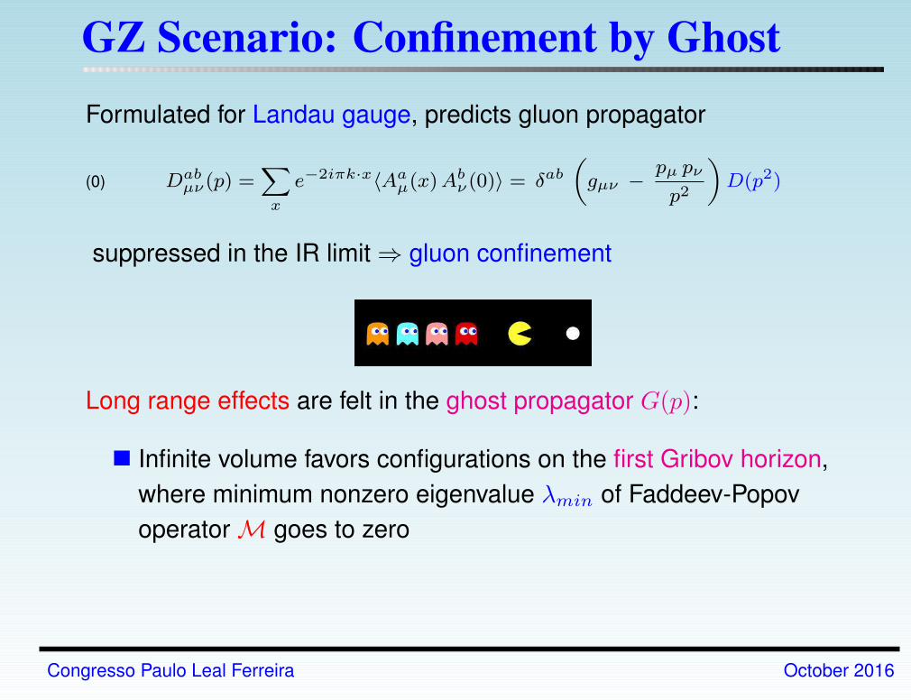
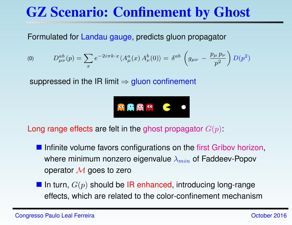
GZ Scenario: Confinement by Ghost
Formulated for Landau gauge, predicts gluon propagator
Dabµν(p) =
∑
x
e−2iπk·x〈Aaµ(x)A
bν(0)〉 = δab
(
gµν −pµ pν
p2
)
D(p2)(0)
suppressed in the IR limit ⇒ gluon confinement
Congresso Paulo Leal Ferreira October 2016
GZ Scenario: Confinement by Ghost
Formulated for Landau gauge, predicts gluon propagator
Dabµν(p) =
∑
x
e−2iπk·x〈Aaµ(x)A
bν(0)〉 = δab
(
gµν −pµ pν
p2
)
D(p2)(0)
suppressed in the IR limit ⇒ gluon confinement
Long range effects are felt in the ghost propagator G(p):
Infinite volume favors configurations on the first Gribov horizon,
where minimum nonzero eigenvalue λmin of Faddeev-Popov
operator M goes to zero
In turn, G(p) should be IR enhanced, introducing long-range
effects, which are related to the color-confinement mechanism
Congresso Paulo Leal Ferreira October 2016
Lattice Landau Gauge
The lattice Landau gauge is imposed by minimizing the functional
S[U ;ω] = −∑
x,µ
Tr Uωµ (x) ,
where ω(x) ∈ SU(N) and Uωµ (x) = ω(x) Uµ(x) ω†(x+ a eµ) is the
lattice gauge transformation.
By considering the relations Uµ(x) = ei a g0 Aµ(x) and ω(x) = ei τ θ(x) ,we can expand S[U ;ω] (for small τ ):
S[U ;ω] = S[U ; 1⊥] + τ S′
[U ; 1⊥](b, x) θb(x)
+τ2
2θb(x)S
′′
[U ; 1⊥](b, x; c, y) θc(y) + . . .
where S′′
[U ; 1⊥](b, x; c, y) = M(b, x; c, y)[A] is a lattice discretization of
the Faddeev-Popov operator −D · ∂ .
Congresso Paulo Leal Ferreira October 2016
Overview of Lattice Results
Note: large-lattice results (L ≈ 27 fm)
Gluon sector:
Gluon propagator is suppressed in the limit p→ 0, while the
real-space propagator violates reflection positivity
Congresso Paulo Leal Ferreira October 2016
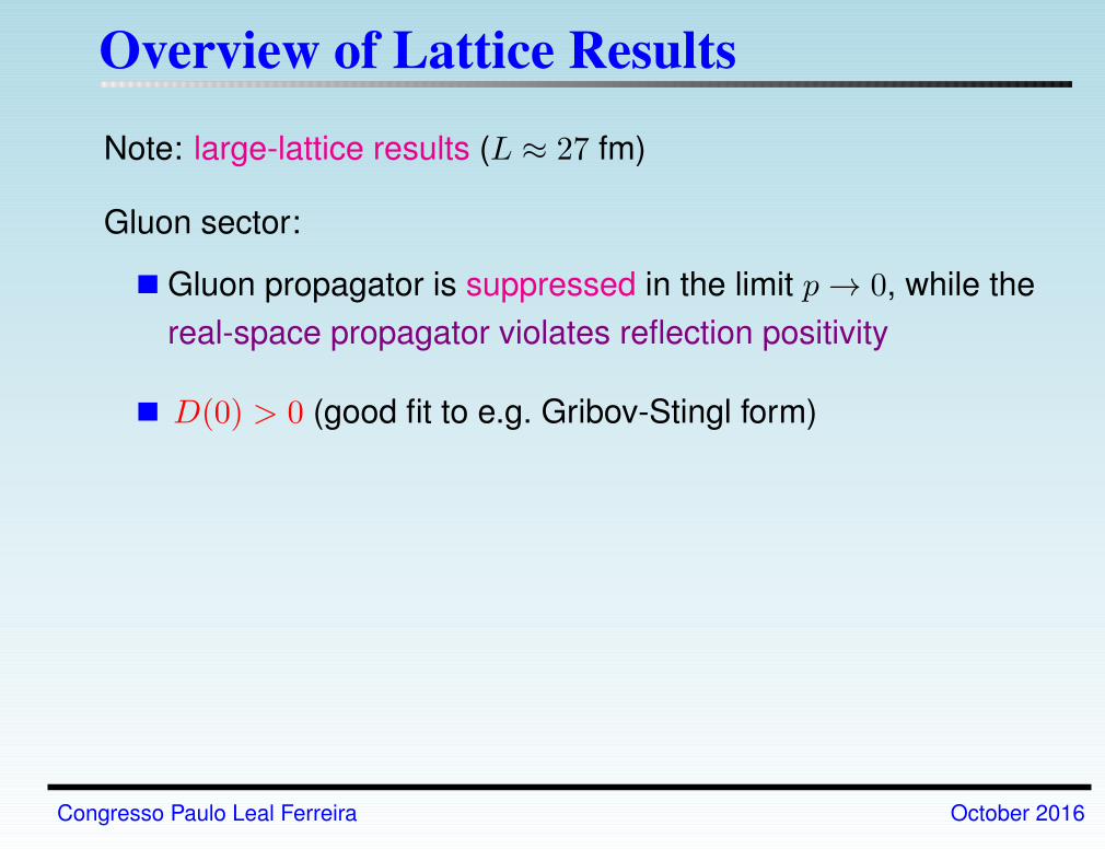
Overview of Lattice Results
Note: large-lattice results (L ≈ 27 fm)
Gluon sector:
Gluon propagator is suppressed in the limit p→ 0, while the
real-space propagator violates reflection positivity
D(0) > 0 (good fit to e.g. Gribov-Stingl form)
Congresso Paulo Leal Ferreira October 2016
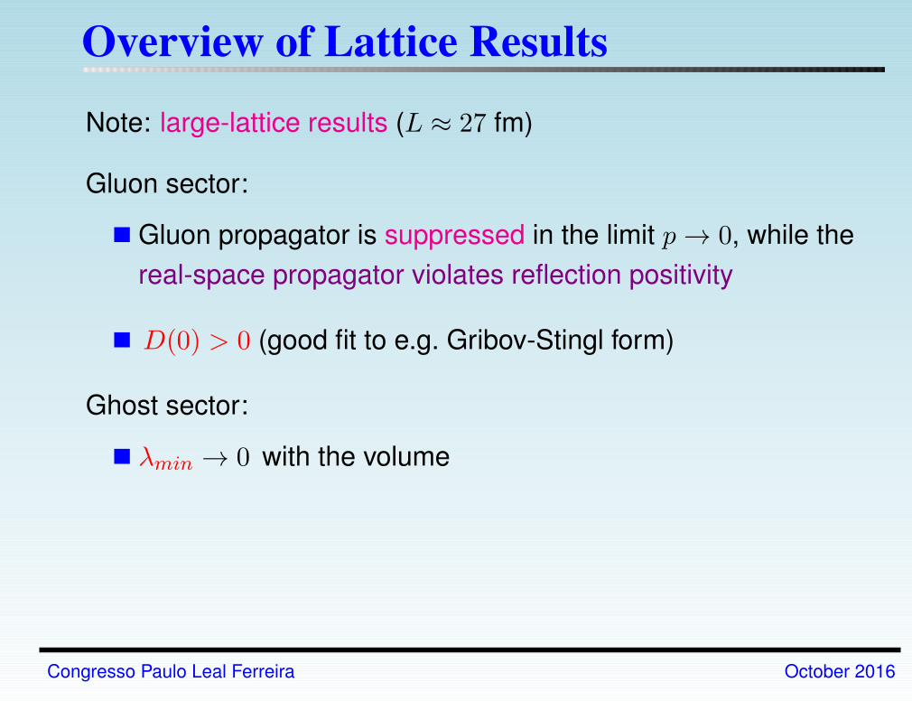
Overview of Lattice Results
Note: large-lattice results (L ≈ 27 fm)
Gluon sector:
Gluon propagator is suppressed in the limit p→ 0, while the
real-space propagator violates reflection positivity
D(0) > 0 (good fit to e.g. Gribov-Stingl form)
Ghost sector:
λmin → 0 with the volume
Congresso Paulo Leal Ferreira October 2016
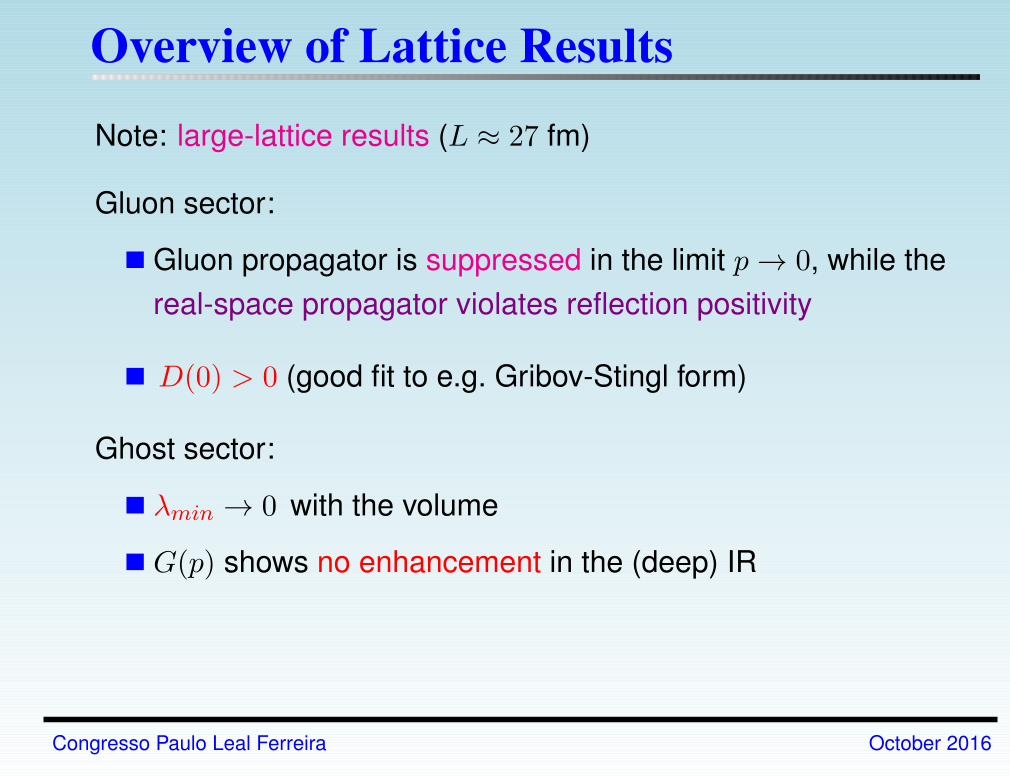
Overview of Lattice Results
Note: large-lattice results (L ≈ 27 fm)
Gluon sector:
Gluon propagator is suppressed in the limit p→ 0, while the
real-space propagator violates reflection positivity
D(0) > 0 (good fit to e.g. Gribov-Stingl form)
Ghost sector:
λmin → 0 with the volume
G(p) shows no enhancement in the (deep) IR
Congresso Paulo Leal Ferreira October 2016
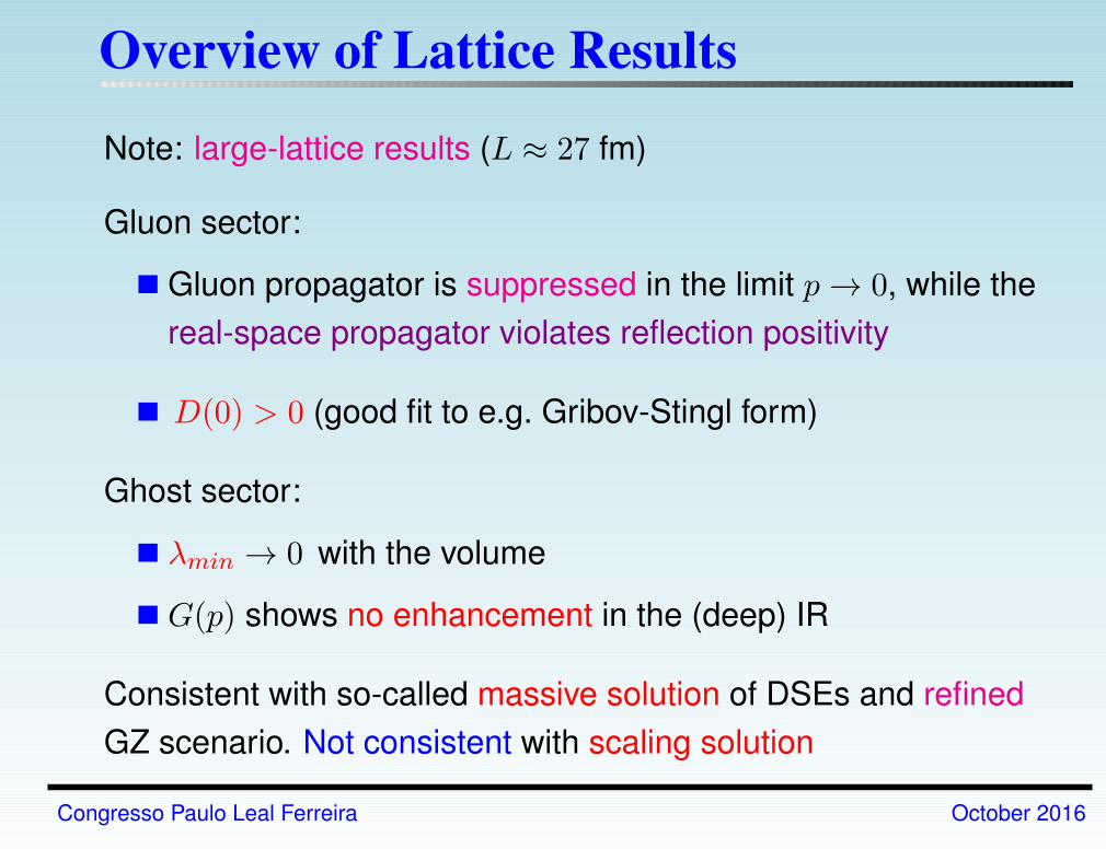
Overview of Lattice Results
Note: large-lattice results (L ≈ 27 fm)
Gluon sector:
Gluon propagator is suppressed in the limit p→ 0, while the
real-space propagator violates reflection positivity
D(0) > 0 (good fit to e.g. Gribov-Stingl form)
Ghost sector:
λmin → 0 with the volume
G(p) shows no enhancement in the (deep) IR
Consistent with so-called massive solution of DSEs and refined
GZ scenario. Not consistent with scaling solution
Congresso Paulo Leal Ferreira October 2016
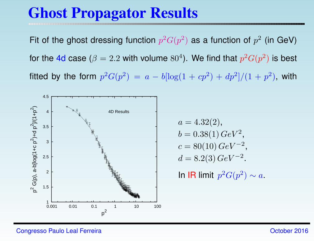
Ghost Propagator Results
Fit of the ghost dressing function p2G(p2) as a function of p2 (in GeV)
for the 4d case (β = 2.2 with volume 804). We find that p2G(p2) is best
fitted by the form p2G(p2) = a − b[log(1 + cp2) + dp2]/(1 + p2), with
1
1.5
2
2.5
3
3.5
4
4.5
0.001 0.01 0.1 1 10 100
p2 G(p
), a
-b[lo
g(1+
c p2 )+
d p2 ]/(
1+p2 )
p2
4D Results
a = 4.32(2),
b = 0.38(1)GeV 2,
c = 80(10)GeV −2,
d = 8.2(3)GeV −2.
In IR limit p2G(p2) ∼ a.
Congresso Paulo Leal Ferreira October 2016
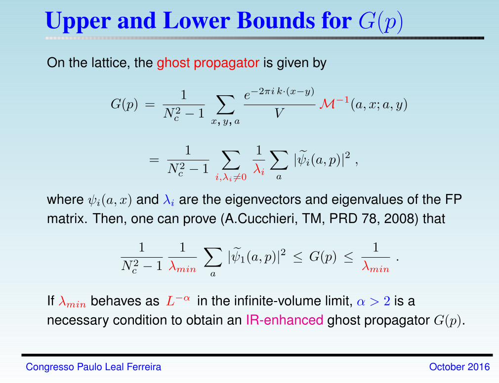
Upper and Lower Bounds for G(p)
On the lattice, the ghost propagator is given by
G(p) =1
N2c − 1
∑
x, y, a
e−2πi k·(x−y)
VM−1(a, x; a, y)
=1
N2c − 1
∑
i,λi 6=0
1
λi
∑
a
|ψi(a, p)|2 ,
where ψi(a, x) and λi are the eigenvectors and eigenvalues of the FP
matrix. Then, one can prove (A.Cucchieri, TM, PRD 78, 2008) that
1
N2c − 1
1
λmin
∑
a
|ψ1(a, p)|2 ≤ G(p) ≤ 1
λmin.
If λmin behaves as L−α in the infinite-volume limit, α > 2 is a
necessary condition to obtain an IR-enhanced ghost propagator G(p).
Congresso Paulo Leal Ferreira October 2016
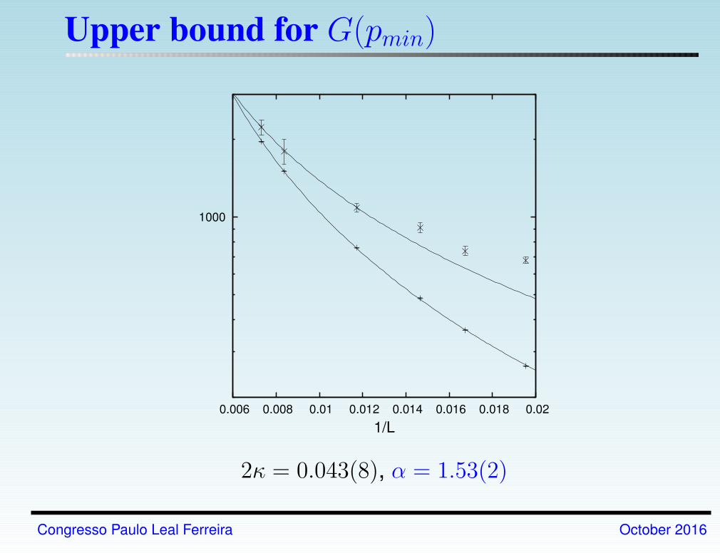
Upper bound for G(pmin)
2κ = 0.043(8), α = 1.53(2)
Congresso Paulo Leal Ferreira October 2016
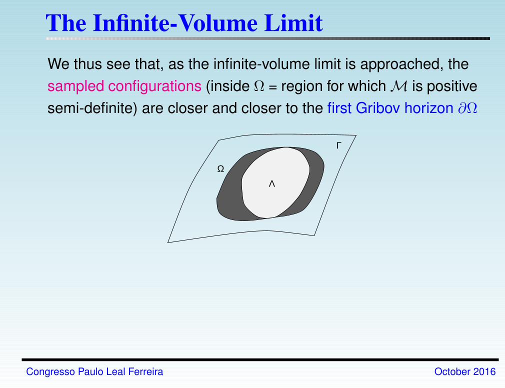
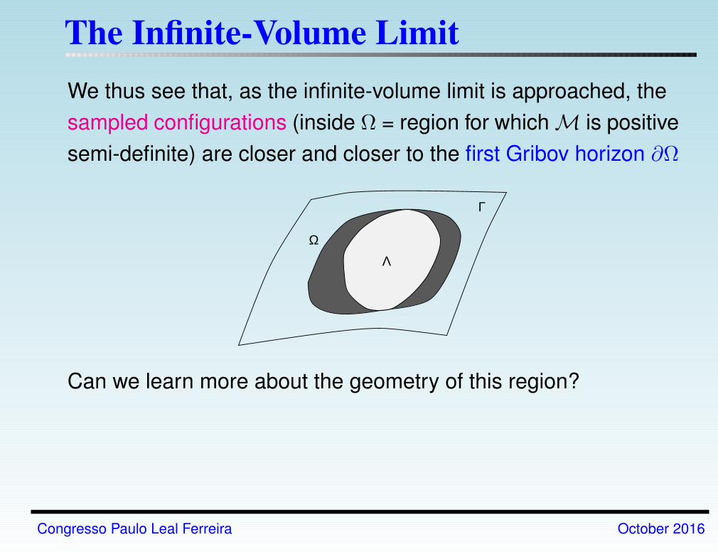
The Infinite-Volume Limit
We thus see that, as the infinite-volume limit is approached, the
sampled configurations (inside Ω = region for which M is positive
semi-definite) are closer and closer to the first Gribov horizon ∂Ω
ΩΛ
Γ
Congresso Paulo Leal Ferreira October 2016
The Infinite-Volume Limit
We thus see that, as the infinite-volume limit is approached, the
sampled configurations (inside Ω = region for which M is positive
semi-definite) are closer and closer to the first Gribov horizon ∂Ω
ΩΛ
Γ
Can we learn more about the geometry of this region?
Congresso Paulo Leal Ferreira October 2016
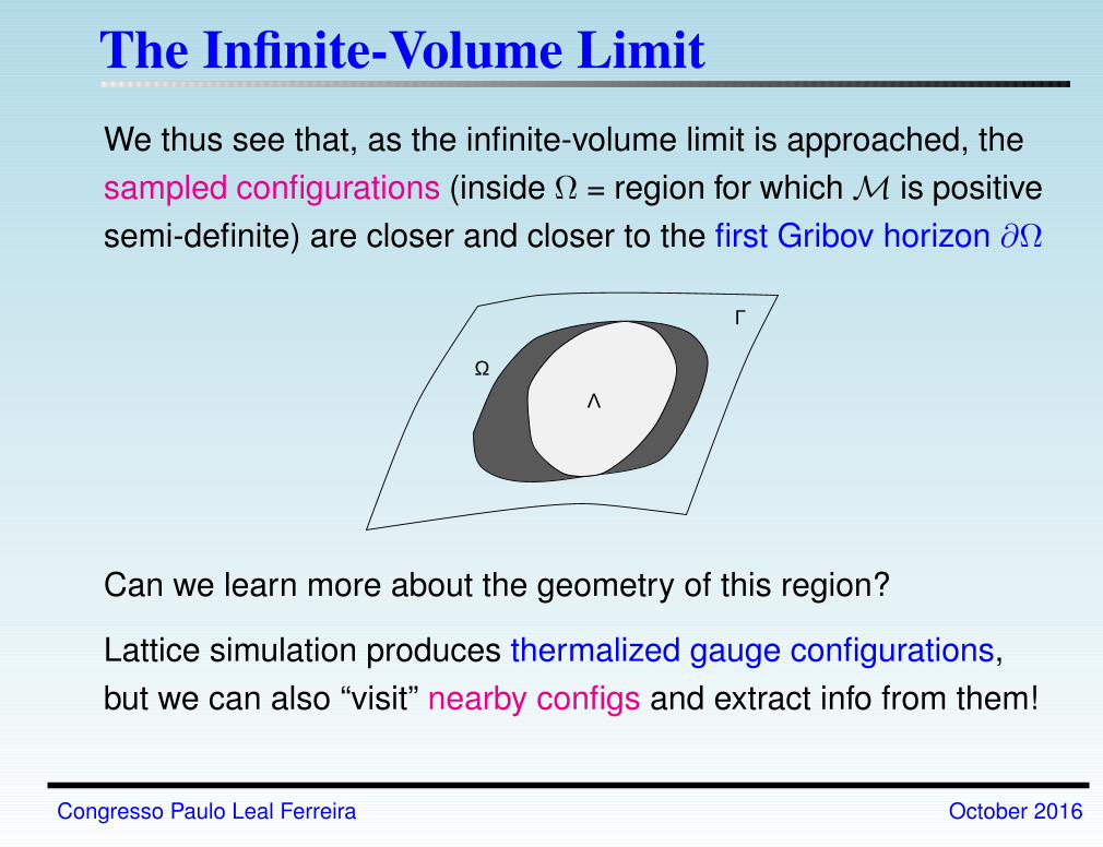
The Infinite-Volume Limit
We thus see that, as the infinite-volume limit is approached, the
sampled configurations (inside Ω = region for which M is positive
semi-definite) are closer and closer to the first Gribov horizon ∂Ω
ΩΛ
Γ
Can we learn more about the geometry of this region?
Lattice simulation produces thermalized gauge configurations,
but we can also “visit” nearby configs and extract info from them!
Congresso Paulo Leal Ferreira October 2016
Reaching (and Crossing!) the Horizon
How many roads have I wondered?
None, and each my own
Behind me the bridges have crumbled
No question of return
Nowhere to go but the horizon
where, then, will I call my home?
The Same Song, Susheela Raman
Congresso Paulo Leal Ferreira October 2016
Reaching (and Crossing!) the Horizon
How many roads have I wondered?
None, and each my own
Behind me the bridges have crumbled
No question of return
Nowhere to go but the horizon
where, then, will I call my home?
The Same Song, Susheela Raman
— They say that communism is just over the horizon. What’s
a horizon?
— A horizon is an imaginary line which continues to recede
as you approach it.
Russian joke from Khrushchev’s time
Congresso Paulo Leal Ferreira October 2016
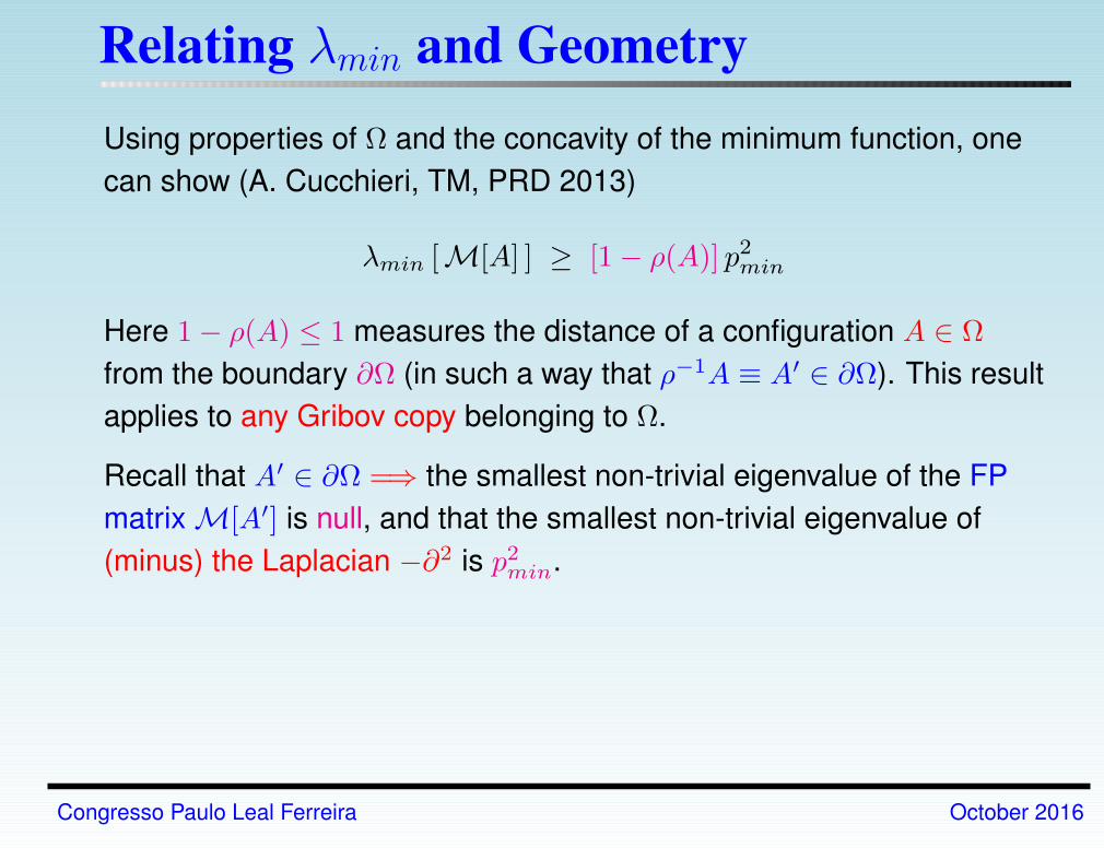
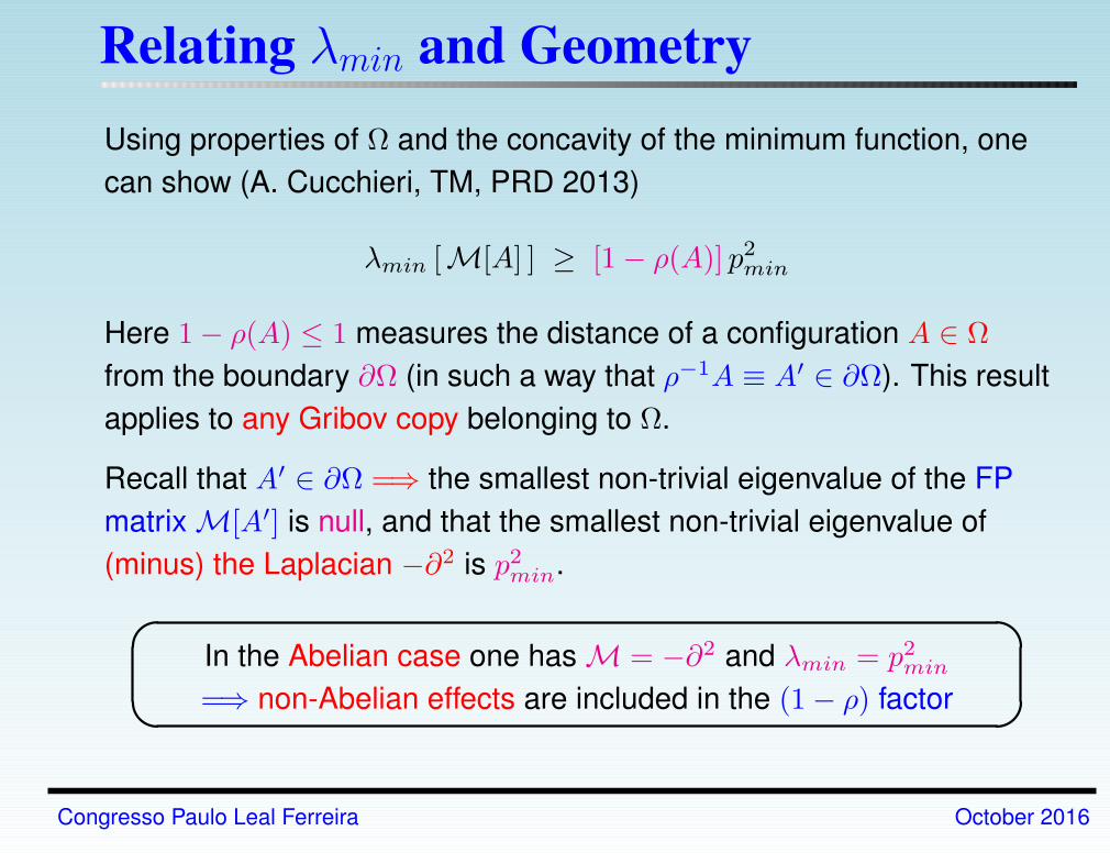
Relating λmin and Geometry
Using properties of Ω and the concavity of the minimum function, one
can show (A. Cucchieri, TM, PRD 2013)
λmin [M[A] ] ≥ [1− ρ(A)] p2min
Here 1− ρ(A) ≤ 1 measures the distance of a configuration A ∈ Ω
from the boundary ∂Ω (in such a way that ρ−1A ≡ A′ ∈ ∂Ω). This result
applies to any Gribov copy belonging to Ω.
Recall that A′ ∈ ∂Ω =⇒ the smallest non-trivial eigenvalue of the FP
matrix M[A′] is null, and that the smallest non-trivial eigenvalue of
(minus) the Laplacian −∂2 is p2min.
Congresso Paulo Leal Ferreira October 2016
Relating λmin and Geometry
Using properties of Ω and the concavity of the minimum function, one
can show (A. Cucchieri, TM, PRD 2013)
λmin [M[A] ] ≥ [1− ρ(A)] p2min
Here 1− ρ(A) ≤ 1 measures the distance of a configuration A ∈ Ω
from the boundary ∂Ω (in such a way that ρ−1A ≡ A′ ∈ ∂Ω). This result
applies to any Gribov copy belonging to Ω.
Recall that A′ ∈ ∂Ω =⇒ the smallest non-trivial eigenvalue of the FP
matrix M[A′] is null, and that the smallest non-trivial eigenvalue of
(minus) the Laplacian −∂2 is p2min.
In the Abelian case one has M = −∂2 and λmin = p2min=⇒ non-Abelian effects are included in the (1− ρ) factor
Congresso Paulo Leal Ferreira October 2016
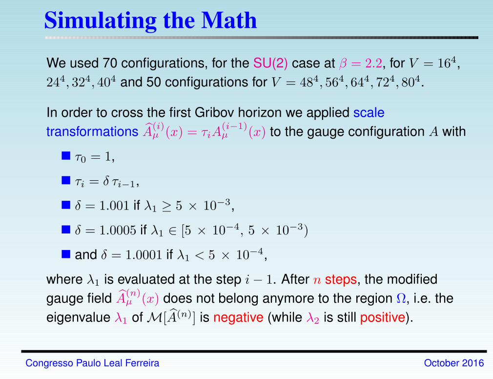
Simulating the Math
We used 70 configurations, for the SU(2) case at β = 2.2, for V = 164,
244, 324, 404 and 50 configurations for V = 484, 564, 644, 724, 804.
In order to cross the first Gribov horizon we applied scale
transformations A(i)µ (x) = τiA
(i−1)µ (x) to the gauge configuration A with
τ0 = 1,
τi = δ τi−1,
δ = 1.001 if λ1 ≥ 5 × 10⁻³,
δ = 1.0005 if λ1 ∈ [5 × 10⁻⁴, 5 × 10⁻³)
and δ = 1.0001 if λ1 < 5 × 10⁻⁴,
where λ1 is evaluated at the step i− 1. After n steps, the modified
gauge field A(n)µ (x) does not belong anymore to the region Ω, i.e. the
eigenvalue λ1 of M[A(n)] is negative (while λ2 is still positive).
Congresso Paulo Leal Ferreira October 2016
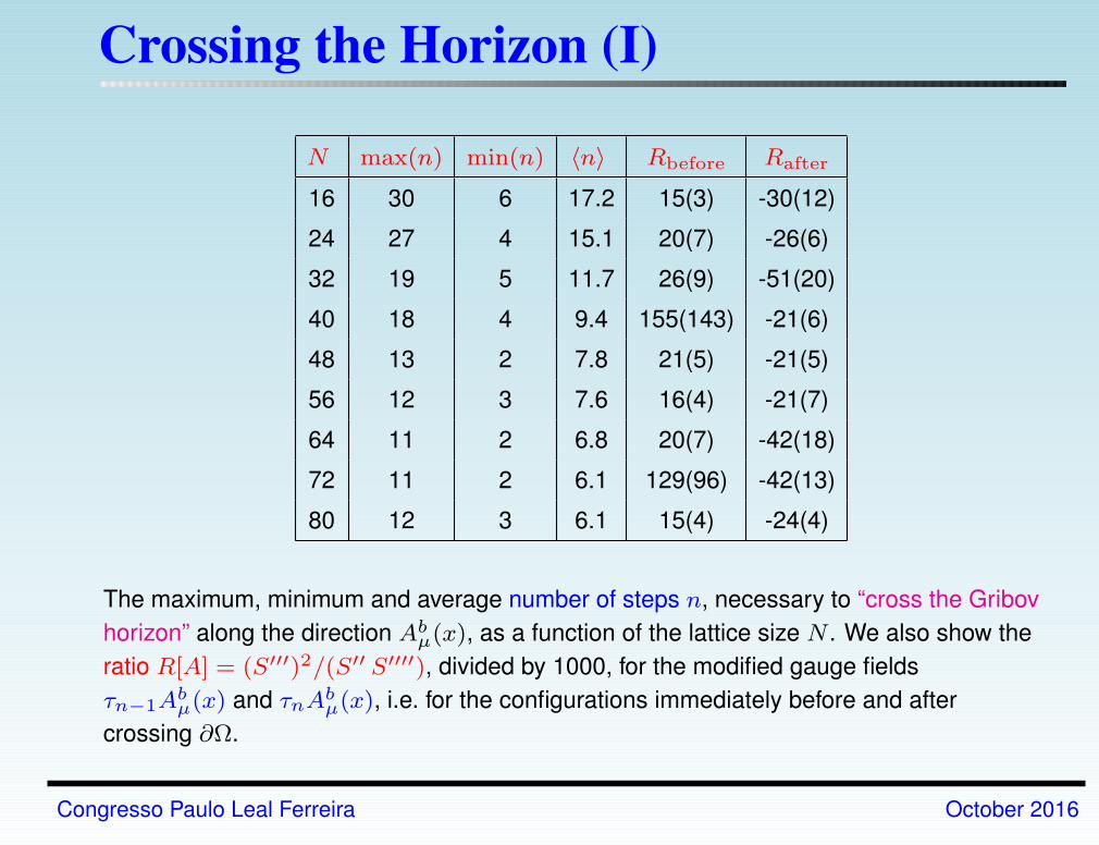
Crossing the Horizon (I)
N max(n) min(n) 〈n〉 Rbefore Rafter
16 30 6 17.2 15(3) -30(12)
24 27 4 15.1 20(7) -26(6)
32 19 5 11.7 26(9) -51(20)
40 18 4 9.4 155(143) -21(6)
48 13 2 7.8 21(5) -21(5)
56 12 3 7.6 16(4) -21(7)
64 11 2 6.8 20(7) -42(18)
72 11 2 6.1 129(96) -42(13)
80 12 3 6.1 15(4) -24(4)
The maximum, minimum and average number of steps n, necessary to “cross the Gribov
horizon” along the direction Abµ(x), as a function of the lattice size N . We also show the
ratio R[A] = (S′′′)2/(S′′ S′′′′), divided by 1000, for the modified gauge fields
τn−1Abµ(x) and τnAb
µ(x), i.e. for the configurations immediately before and after
crossing ∂Ω.
Congresso Paulo Leal Ferreira October 2016
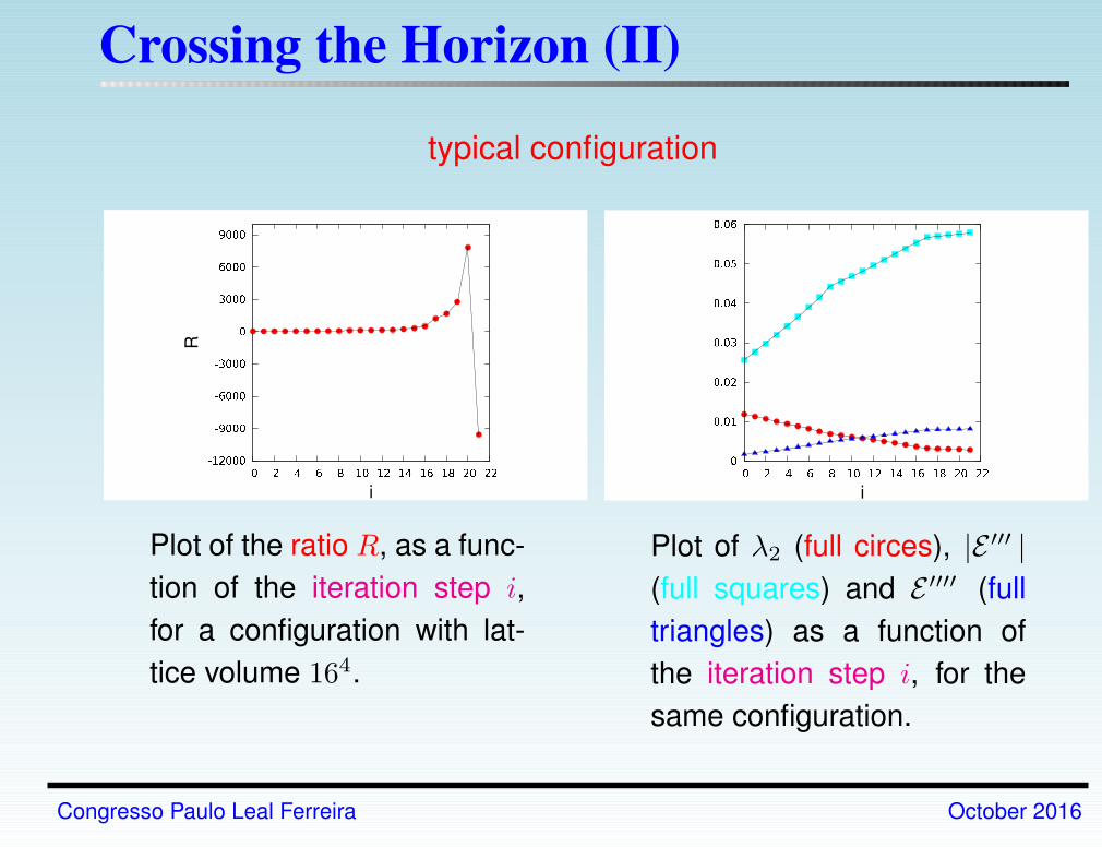
Crossing the Horizon (II)
typical configurationR
i
Plot of the ratio R, as a func-
tion of the iteration step i,
for a configuration with lat-
tice volume 164.
i
Plot of λ2 (full circes), |E ′′′ |(full squares) and E ′′′′ (full
triangles) as a function of
the iteration step i, for the
same configuration.
Congresso Paulo Leal Ferreira October 2016
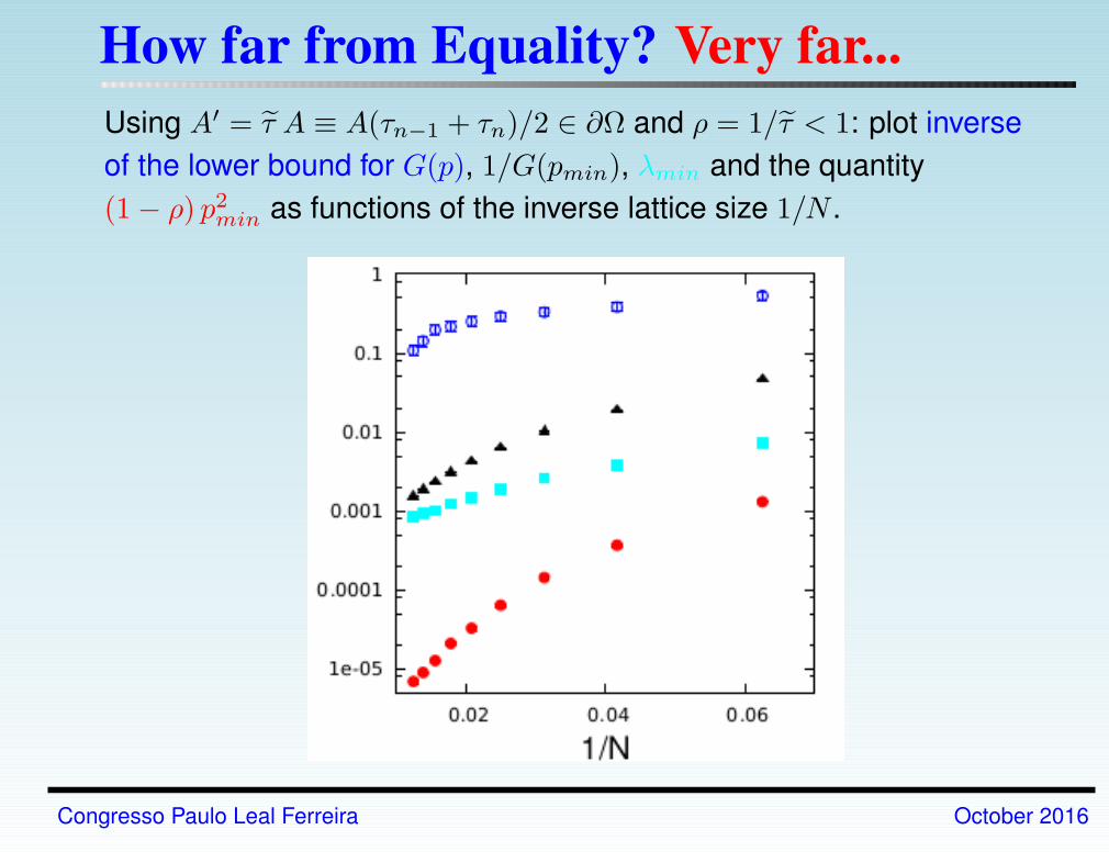
How far from Equality? Very far...Using A′ = τ A ≡ A(τn−1 + τn)/2 ∈ ∂Ω and ρ = 1/τ < 1: plot inverse
of the lower bound for G(p), 1/G(pmin), λmin and the quantity
(1− ρ) p2min as functions of the inverse lattice size 1/N .
Congresso Paulo Leal Ferreira October 2016
So?
Eigenvalues are not nontrivial...
Congresso Paulo Leal Ferreira October 2016
So?
Eigenvalues are not nontrivial...
Now notice that:
The inequality λmin [M[A] ] ≥ [1− ρ(A)] p2min becomes an
equality if and only if the eigenvectors corresponding to the
smallest nonzero eigenvalues of M[A] and −∂2 coincide
=⇒ unlikely...
Congresso Paulo Leal Ferreira October 2016
So?
Eigenvalues are not nontrivial...
Now notice that:
The inequality λmin [M[A] ] ≥ [1− ρ(A)] p2min becomes an
equality if and only if the eigenvectors corresponding to the
smallest nonzero eigenvalues of M[A] and −∂2 coincide
=⇒ unlikely...
Our results show that the eigenvector ψmin is very different from
the plane waves corresponding to pmin
This should serve to illustrate the (nontrivial) non-enhancement
of G(p) in the IR
Congresso Paulo Leal Ferreira October 2016
Conclusions
Using Monte Carlo simulations:
We’ve tested ghost enhancement as predicted in
Gribov-Zwanziger confinement scenario: ghost responds to
hadronic scale, but no enhancement in the deep IR
Congresso Paulo Leal Ferreira October 2016
Conclusions
Using Monte Carlo simulations:
We’ve tested ghost enhancement as predicted in
Gribov-Zwanziger confinement scenario: ghost responds to
hadronic scale, but no enhancement in the deep IR
We’ve ventured outside the region Ω (away from sampled
configurations) to probe the geometry of the Gribov horizon
Combination of trivial eigenvalue and nontrivial eigenvectors
associated with observed lack of ghost enhancement in the
deep IR
Congresso Paulo Leal Ferreira October 2016

Conclusions
Using Monte Carlo simulations:
We’ve tested ghost enhancement as predicted in
Gribov-Zwanziger confinement scenario: ghost responds to
hadronic scale, but no enhancement in the deep IR
We’ve ventured outside the region Ω (away from sampled
configurations) to probe the geometry of the Gribov horizon
Combination of trivial eigenvalue and nontrivial eigenvectors
associated with observed lack of ghost enhancement in the
deep IR
We’ve come a long way... in discarding things we thought
we knew about confinement
Congresso Paulo Leal Ferreira October 2016


![v } - Home - AVESaves.org.br/wp-content/uploads/2014/07/53bec7f06501b.pdf · Diretório Pastoral Litúrgico-Sacramental e Ministerial µ u ] } µ u ] } /EdZK h K X X X X X X X X X](https://img.document.onl/doc/110x75/5be9a3f709d3f2ce778d3b6e/v-home-diretorio-pastoral-liturgico-sacramental-e-ministerial-u-.jpg)