Universidade Nova de LisboaFaculdade de Ciências e Tecnologia

Departamento de Informática

Dissertação de Mestrado

Mestrado em Engenharia Informática

Solving Colored Nonograms

Luís Pedro Canas Ferreira Mingote(aluno nº 29634)

2º Semestre de 2008/092009

Universidade Nova de LisboaFaculdade de Ciências e Tecnologia

Departamento de Informática

Dissertação de Mestrado

Solving Colored Nonograms

Luís Pedro Canas Ferreira Mingote(aluno nº 29634)

Orientador: Prof. Doutor Francisco de Azevedo

Trabalho apresentado no âmbito do Mestrado em Engen-haria Informática, como requisito parcial para obtenção dograu de Mestre em Engenharia Informática.

2º Semestre de 2008/092009

Dedication

To my wife Marta. Without her incentive, support, patience, inspiration and family dedica-tion I could never have finished this work.

To my daughters Margarida and Matilde. That this work may be an incentive to always seekto increase their knowledge.

v

Acknowledgements

I would like to thank Prof. Francisco de Azevedo for his time and orientation. I cannotthank him enough for all the patience in reading, understanding and proposing improvementsto my writings.

I also would like to thank Prof. Paula Amaral, from the Mathematics Department, for mak-ing available CPLEX for testing.

Thank you Alberto Bigotte de Almeida for all your support and help in the beginning of thisendeavor.

I would also like to thank all my family for their support and incentive.

I would like to thank my late mother, Maria do Céu, for the education she gave me and forinstilling the will to always be a better person and always widen my knowledge.

I would also like to remember my late grandfather who played a significant role in myeducation.

vii

Resumo

Nesta dissertação aprofundamos o estudo da resolução de nonogramas coloridos utilizandoProgramação Linear Inteira (PLI). As formas conhecidas de resolução deste tipo de problemassão a força-bruta, o método iterativo e PLI.

A nossa aproximação generaliza a utilizada por Robert A. Bosch desenvolvida para, apenas,nonogramas a preto e branco, tornando assim disponível uma solução nova e universal para aresolução de nonogramas utilizando PLI.

Sendo as implementações do método iterativo as que apresentam melhores resultados aonível do desempenho, desenvolvemos também um método híbrido que combina esta aproxi-mação e PLI.

Estes puzzles têm, muitas vezes, várias soluções. A forma de as encontrar pelo modo iter-ativo é uma pesquisa em árvore com retrocesso. De forma a encontrar as restantes soluções nanossa aproximação aplicamos um algoritmo que utiliza um corte binário para excluir soluçõesjá conhecidas.

Para efeito de testes comparativos entre as diversas aproximações ao problema, desenvolve-mos um gerador de nonogramas que permite definir a resolução do puzzle, o seu número decores e a densidade (número de células pintadas vs. resolução).

Finalmente comparamos o desempenho da nossa aproximação para resolver nonogramascoloridos com o da aproximação interativa.

Palavras-chave: Nonograma, pintar-por-números, PLI, Programação Linear Inteira

ix

Abstract

In this thesis we deepen the study of colored nonogram solving using Integer Linear Pro-gramming (ILP). The known methods for solving this kind of problems are the depth-first search(brute-force) one, the iterative one and the ILP one.

Our approach generalizes the one used by Robert A. Bosch which was developed for blackand white nonograms only, thus providing a new universal solution for solving nonograms usingILP.

Since the iterative implementations are the ones that present better performance results, wealso developed a hybrid method that combines this approach and the ILP one.

These puzzles often have more than one solution. The way to find them using the iterativemethod is to make a tree search with backtracking. In order to find the remaining solutionsusing our approach, it is necessary to apply an algorithm that uses a binary cut to excludealready known solutions.

In order to perform comparative tests between approaches, we developed a nonogram gen-erator that allows us to define the resolution of the puzzle, its number of colors and its density(number of painted cells vs. resolution).

Finally we compare the performance of our approach in solving colored nonograms againstthe iterative one.

Keywords: Nonogram, paint-by-numbers, ILP, Integer Linear Programming

xi

Contents

1 Introduction 11.1 Context 11.2 Problem Description 1

1.2.1 Initial problems 11.2.2 Nonograms 1

1.2.2.1 Black and White Nonograms 21.2.2.2 Colored Nonograms 2

1.3 Scope of work and main contributions 31.4 Document’s structure 4

2 Nonograms 52.1 Black and white Nonograms 5

2.1.1 Simple boxes 62.1.2 Punctuating 72.1.3 Simple spaces 82.1.4 Mercury 92.1.5 Forcing 92.1.6 Glue 92.1.7 Joining and splitting 10

2.2 Colored Nonograms 112.2.1 Simple boxes 122.2.2 Punctuating 142.2.3 Simple spaces 142.2.4 Mercury 152.2.5 Forcing 152.2.6 Glue 162.2.7 Joining and splitting 16

2.3 Approaches to solving Nonograms 172.3.1 Depth-first search (brute-force) 182.3.2 Iterative approach 192.3.3 Integer Linear Programming approach 21

3 An ILP model for solving Colored Nonograms 233.1 Model Description 23

3.1.1 Notation 233.1.2 Variables 243.1.3 Block constraints 253.1.4 Double Coverage Constraints 26

xiii

xiv

3.1.5 Objective Function 283.1.6 Pre-conditions 28

3.2 Instantiation to Black and White Nonograms 293.3 Finding Multiple Solutions 293.4 Hybrid model 30

4 Results 334.1 Pure ILP approach 334.2 Nonogram Generator 344.3 Hybrid ILP approach 36

5 Conclusions and Future Work 45

A Full Results 47

B Results by block density 59

C Objective function constraint results 63C.1 Graphic Analysis 63C.2 Full Results 64

D Nonogram File Formats 71D.1 Bosch based file format 71D.2 Olšák file format 76D.3 Hett based file format 77

List of Figures

1.1 Black and white nonogram example (unsolved: left, solved: right) 21.2 Colored Nonogram Example - "Fall" from [2] 3

2.1 Black and white nonogram example 62.2 Example for the method Simple boxes in black and white nonograms 72.3 Example for the method Punctuating 82.4 Example 1 for the method Simple spaces applied to a black and white nonogram 82.5 Example 2 for the method Simple spaces applied to a black and white nonogram 82.6 Example for the method Mercury 92.7 Example for the method Forcing 102.8 Example for the method Glue 102.9 Example for the method Joining and splitting applied to a black and white nono-

gram 102.10 Solving a black and white Nonogram Example 112.11 Solving a black and white Nonogram Example — after last (horizontal) iteration 122.12 Example 1 for the method Simple boxes 132.13 Example for the method Punctuating 142.14 Example 1 for the method Simple spaces 142.15 Example 2 for the method Simple spaces 152.16 Example for the method Mercury 152.17 Example for the method Forcing 162.18 Example for the method Glue 162.19 Example for the method Joining and splitting 172.20 Solving a Colored Nonogram Example — "Fall" from [2] 172.21 Solving a Colored Nonogram Example — "Fall" from [2] 182.22 Solving a Colored Nonogram Example — "Fall" from [2] — After final (hori-

zontal) iteration 192.23 Depth-first search — all possibilities for a line 20

4.1 Generated nonogram 354.2 ILP: Average resolution by density (20x20) and number of solved puzzles 394.3 Iterative: Average resolution by density (20x20) and number of solved puzzles 394.4 ILP: Average resolution by density (40x60) and number of solved puzzles 404.5 Iterative: Average resolution by density (40x60) and number of solved puzzles 414.6 ILP: Average resolution by density (100x100) and number of solved puzzles 414.7 Iterative: Average resolution by density (100x100) and number of solved puzzles 424.8 Hybrid ILP vs. Pure ILP comparison (20x20) 43

B.1 ILP: Average resolution time by block density, in seconds (20x20) 59xv

xvi

B.2 Iterative: Average resolution time by block density, in seconds (20x20) 59B.3 ILP: Average resolution time by block density, in seconds (40x60) 60B.4 Iterative: Average resolution time by block density, in seconds (40x60) 60B.5 ILP: Average resolution time by block density, in seconds (100x100) 60B.6 Iterative: Average resolution time by block density, in seconds (100x100) 61

C.1 Comparison of adding the objective function constraint (20x20) 63C.2 Comparison of adding the objective function constraint (40x60) 64

List of Tables

2.1 Experimental Results (in seconds) 21

4.1 Experimental Results (in seconds) 334.2 Results of adding equation (4.1) to ILP (in seconds) 344.3 Number of solved puzzles by method and dimension 374.4 Number of solved puzzles by method, dimension and density 374.5 Number of solved puzzles by method and density 384.6 Average time to solve a puzzle by dimension 384.7 Average time to solve a puzzle by density 38

A.1 Full Results (in seconds) 48

C.1 Objective Function Constraint Full Results (in seconds) 64

xvii

1 . Introduction

1.1 Context

The work hereby presented was developed during the Master Program in Computer Sci-ence Engineering (Bologna second cycle), under the original theme "Solving Problems fromCSPLib".

1.2 Problem Description

1.2.1 Initial problems

Initially, the purpose of this work was to solve problems from CSPLib (www.csplib.org), aknown library of problems for modeling and solving. Given the lack of knowledge about themajority of the existing problems and our interest in exploring and solving new problems, thusbroadening our knowledge base, we decided to analyze the following five:

• prob012: Nonograms

• prob020: Darts tournament

• prob022: Bus driver scheduling

• prob032: Maximum density still life

• prob037: Peg solitaire

Although some work was done on problem "prob032 - Maximum density still life", specifi-cally the implementation of the Bucket Elimination algorithm by [11], we decided to deepen thestudy about problem "prob012 - Nonograms" since it appeared to us that there were approachesthat had not been explored, specially to what concerns colored nonograms.

1.2.2 Nonograms

Nonograms are a popular kind of puzzle whose name varies from country to country, includ-ing Paint by Numbers and Griddlers. The goal is to fill cells of a grid in a way that contiguousblocks of the same color satisfy the clues, or restrictions, of each line or column.

According to Wikipedia [21], these kind of puzzles were created in 1987 by Non Ishida,a Japanese graphics editor, and Tetsuya Nishio, a professional Japanese puzzler, at the sametime and with no relation whatsoever. Soon after, nonograms started appearing in Japanesepuzzle magazines and later as electronic games. Today, magazines with nonogram puzzles arepublished in several countries and are available as electronic games in a variety of platforms.

Ueda e Nagao prove in [19] that this problem is NP-Complete.1

2

1.2.2.1 Black and White Nonograms

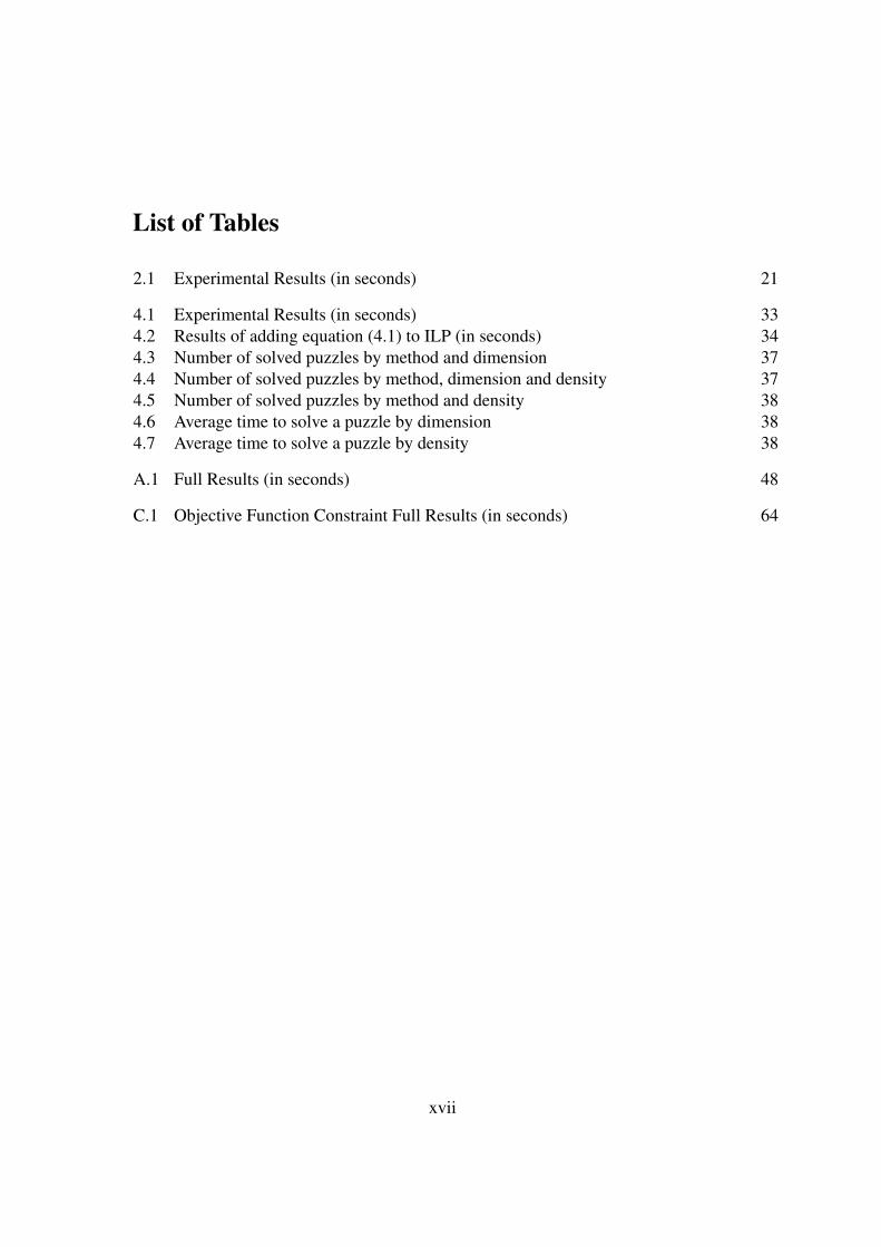
In black and white nonograms the clues indicate the sequence of contiguous blocks of cellsto be filled (e.g. the clue 3,1,2 indicates that there is a block of 3 contiguous cells, followedby a sequence of one or more empty cells, then a block of one cell filled, followed by anothersequence of one or more empty cells, finally followed by a sequence of two filled cells in thatrow or column). Figure 1.1 shows an example of a black and white nonogram (unsolved, to theleft, solved, to the right).

Figure 1.1 Black and white nonogram example (unsolved: left, solved: right)

Known approaches to solving black and white nonograms are the depth-first search (brute-force) one, the iterative one, the ILP one by Bosch [7] and a genetic algorithm by WouterWiggers [20].

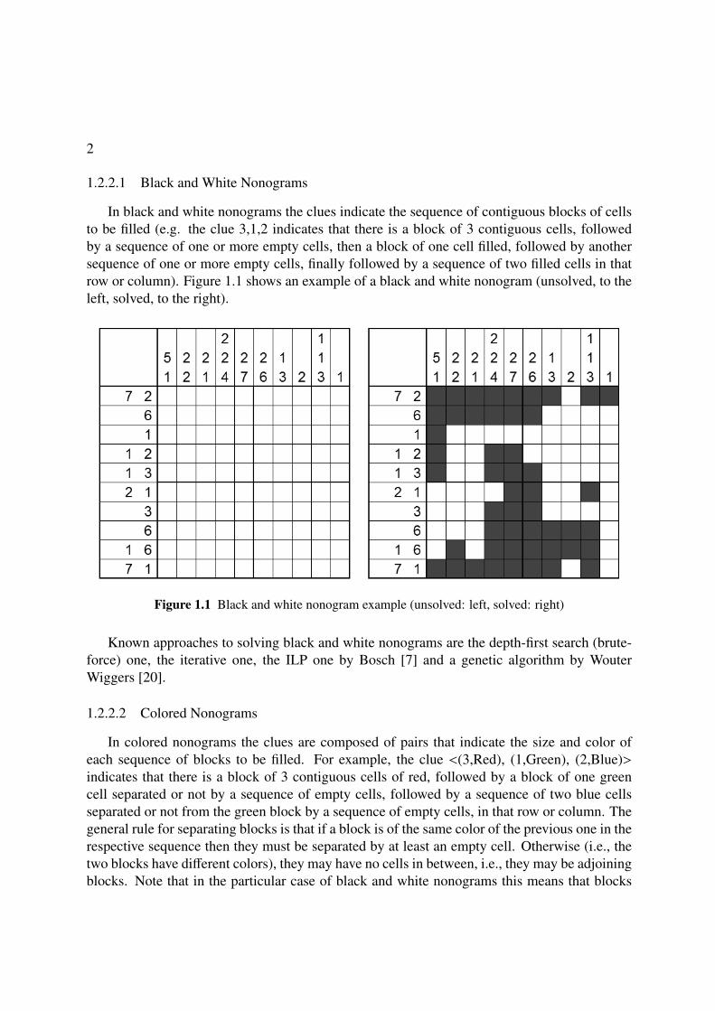
1.2.2.2 Colored Nonograms

In colored nonograms the clues are composed of pairs that indicate the size and color ofeach sequence of blocks to be filled. For example, the clue <(3,Red), (1,Green), (2,Blue)>indicates that there is a block of 3 contiguous cells of red, followed by a block of one greencell separated or not by a sequence of empty cells, followed by a sequence of two blue cellsseparated or not from the green block by a sequence of empty cells, in that row or column. Thegeneral rule for separating blocks is that if a block is of the same color of the previous one in therespective sequence then they must be separated by at least an empty cell. Otherwise (i.e., thetwo blocks have different colors), they may have no cells in between, i.e., they may be adjoiningblocks. Note that in the particular case of black and white nonograms this means that blocks

3

in a sequence must always be separated by at least one empty cell. Figure 1.2 represents anexample of a colored nonogram with 10 lines by 8 columns with 3 colors.

Figure 1.2 Colored Nonogram Example - "Fall" from [2]

1.3 Scope of work and main contributions

Within the scope of this work, colored nonograms were studied in order to develop an IntegerLinear Programming model for solving them. This model is based on the one provided byBosch in [7] for black and white nonograms and generalizes it so it can solve both black andwhite and colored puzzles. Bosch’s file format was also adapted to colored nonograms and ourimplementation also supports lines with no clues.

Since the iterative approach is the one that presents the best results, according to Jan Wolterin [23] and according to the tests we performed (shown ahead), we decided to build an hybridmodel that integrates both approaches.

In order to compare results of both our models and the iterative one, we built a nonogramgenerator that can generate puzzles given a resolution (width × height), a number of colors anda density (global or by color).

This allowed us to broaden the sample set used in comparing the different approaches to

4

solving nonograms thus providing a deeper comparison between them with tests over severalinstances of different dimensions and difficulty.

Our ILP approach was also enhanced in order to obtain more solutions to the same problem,if applicable. This enhancement was accomplished by simplifying a known algorithm that findsmultiple solutions in order to make it more efficient to this specific problem.

In summary, the main contributions of this work are:

• An ILP model for solving colored nonograms;

• A nonogram instance generator;

• An hybrid implementation between the iterative approach and our ILP approach for col-ored nonogram solving.

• A more systematic study of the different nonogram solving approaches

• An adaptation of an algorithm that obtains multiple solutions to an ILP problem, with asimplification that makes it more efficient to specific problems

1.4 Document’s structure

This document is organized in the following way: In Chapter 2 nonograms (both black andwhite and colored) are described in full and the best known approaches are detailed.

In Chapter 3 the ILP model we developed to solve colored nonograms is described, includ-ing a demonstration that this model corresponds to the one by Bosch in [7] for black and whitenonograms. It is also shown how to apply a simple technique in order to find additional solu-tions in case the first solution obtained for a puzzle is not unique. A description of the hybridapproach between the iterative approach and the hereby presented ILP model is also described.

In Chapter 4 results from the presented solutions are compared to its iterative counterpart.A description of the nonogram generator is also presented.

In Chapter 5 the results of the previous chapter are analyzed and the conclusions of thiswork are presented. We also suggest some future work based on the one presented here.

In Appendix A a table with the result of all tests is shown.In Appendix D an example of each file format used is shown.

2 . Nonograms

In the previous chapter a brief description of nonograms was presented. In this one a moredetailed explanation about nonograms is shown.

Nonograms are a popular kind of puzzle whose name varies from country to country,including Paint by Numbers and Griddlers. The goal is to fill cells of a grid in a way thatcontiguous blocks of the same color satisfy the clues, or restrictions, of each line or column.

According to Wikipedia [21], these kind of puzzles were created in 1987 by Non Ishida,a Japanese graphics editor, and Tetsuya Nishio, a professional Japanese puzzler, at the sametime and with no relation whatsoever. Soon after, nonograms started appearing in Japanesepuzzle magazines and later as electronic games. Today, magazines with nonogram puzzles arepublished in several countries and are available as electronic games in a variety of platforms.

The most common nonograms are black and white, but they exist also in colors. In fact,black and white nonograms are a specialization of colored nonograms, i.e., are two colorednonograms.

Also there is a different kind of nonogram — called triddlers — in which cells are triangles.In this kind of puzzles we have three sets of clues instead of only two. These puzzles can alsoexist in multiple colors.

Ueda e Nagao prove in [19] that the nonogram problem is NP-Complete.

2.1 Black and white Nonograms

In black and white nonograms the clues indicate the sequence of contiguous blocks of cellsto be filled (e.g. the clue 3,1,2 indicates that there is a block of 3 contiguous cells, followedby a sequence of one or more empty cells, then a block of one cell filled, followed by anothersequence of one or more empty cells, finally followed by a sequence of two filled cells in thatrow or column). Figure 1.1 shows an example of a black and white nonogram (unsolved, to theleft, solved, to the right).

According to Wikipedia [21], in order to solve this kind of puzzle it is necessary todetermine which cells will be filled (black) and which will be empty (white). Determiningwhich cells will be empty is as important as determining which will be filled because the formerwill help delimiting the solutions for the blocks of each line or column1.

Simpler puzzles, like the one shown in figure 2.10, can usually be solved by applying thefollowing methods to each line at a time.

1For the sake of simplicity, from this point forward, only lines will be mentioned, since the reasoning is thesame for columns.

5

6

Figure 2.1 Black and white nonogram example

2.1.1 Simple boxes

At the beginning of the solution, when there are no filled cells, for each block bi ∈ {b1, ...,bB} ineach row, the space available S (bi) for it is determined, assuming that the remaining blocks aremoved closer to the extremities of the grid as possible (previous blocks to the left and subsequentblock to the right). bi represents a set of filled cells in sequence (vector). The value for S (bi)can be calculated using equation 2.1, where L represents the size of the line, B represents thenumber of blocks on the line and T (bi) represents the size of bi.

S (bi) = L−B+ 1−B∑

k,i

T (bk) (2.1)

It is also possible to know for each block what is the potential first cell that it can occupythrough equation 2.2, where bi[1] is block’s bi first cell position in the grid.

bi[1] =

{1 ; i = 1bi−1[1] + T (bi−1) + 1 ; i > 1 (2.2)

Within this set of cells it is possible to determine which subset is actually filled by analyzingthe extremities of the solution, i.e., sliding the block as far to the left as possible and then asfar to the right as possible and checking which cells are common to both solutions. In this way,equation 2.3 gives the size of this sub-block, where T (si) is the size of the sub-block si that can

7

be determined for block bi.

T (si) = 2T (bi)−S (bi) (2.3)

In the same way, it is possible to obtain the first cell (consequently the remaining) of thissub-block through equation 2.4, where si[1] is the position of the first cell of sub-block si.

si[1] = bi[1] + S (bi)−T (bi) ; T (si) > 0 (2.4)

Figure 2.2 Example for the method Simple boxes in black and white nonograms

As an example, for the 10th line of the puzzle shown in figure 2.1, L = 10, B = 2, T (b1) = 7and T (b2) = 1. Therefore the space available for the first block is S (b1) = 10− 2 + 1− 1 = 8and S (b2) = 10−2 + 1−7 = 2. The leftmost indexes each can occupy are b1[1] = 1 and b2[1] =

1 + 7 + 1 = 9.As for the sub-blocks of cells that can be filled at this point, T (s1) = 2× 7− 8 = 6 and

T (s2) = 2× 1− 2 = 0, i.e., it is not possible to fill, for now, any cell in respect to the secondblock, but it is possible to fill six cells with respect to the first one. It is yet to determine thestarting cell of the first and second sub-blocks: s1[1] = 1 + 8−7 = 2, i.e., it is possible to fill, atthis point, cells 2 through 7 of that line.

Figure 2.2, from line 10 of the puzzle shown in figure 2.1, exemplifies this method for a size10 line with with two blocks of sizes 7 and 1.

2.1.2 Punctuating

In order to solve the puzzle it is also very important to enclose with empty cells the extrem-ities of each completed block, immediately, as described in the method Simple spaces. Precisepunctuating usually leads to more Forcing and can be vital to finishing the puzzle.

Figure 2.3 exemplifies this method for column 9 of the puzzle shown in figure 2.1.

8

Figure 2.3 Example for the method Punctuating

2.1.3 Simple spaces

The purpose of this method is to find cells that can not be filled by any block due to theconstraints imposed by filled cells. For example, a block that is already complete may have atleast an empty cell to its left and at least another one to its right, unless it is adjacent to thebeginning or the end of the line.

Figure 2.4 from column 8 of the puzzle shown in figure 2.1 shows an example of this method.

Figure 2.4 Example 1 for the method Simple spaces applied to a black and white nonogram

In figure 2.5, based on one from Wikipedia, a more illustrative example of this method isshown.

Figure 2.5 Example 2 for the method Simple spaces applied to a black and white nonogram

First, clue 1 is complete which means that there will be an empty cell to its left and anotherto its right (Punctuating). Then, from clue 3 it is possible to conclude that its block can only

9

expand between the second and the sixth cell because it has to include the fourth cell. Thismeans that cells 1 and 7 will be empty.

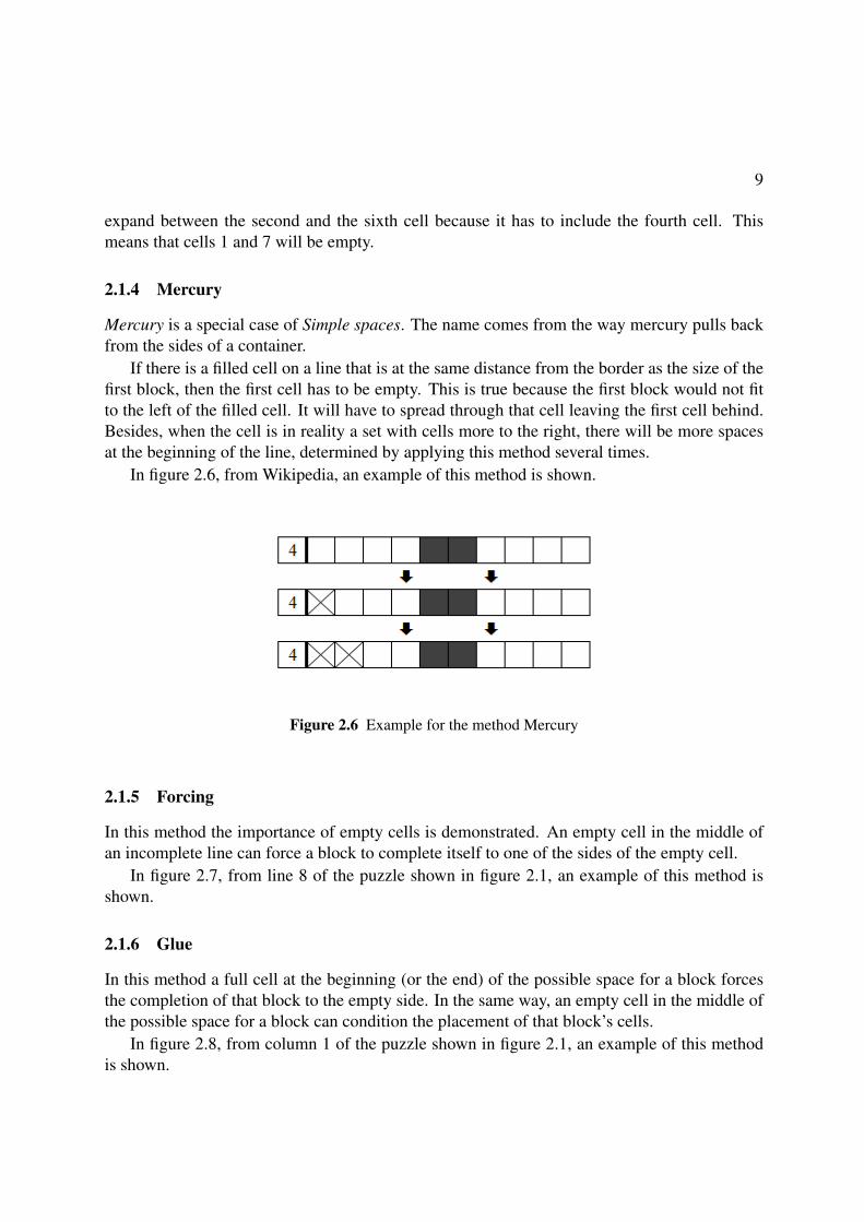
2.1.4 Mercury

Mercury is a special case of Simple spaces. The name comes from the way mercury pulls backfrom the sides of a container.

If there is a filled cell on a line that is at the same distance from the border as the size of thefirst block, then the first cell has to be empty. This is true because the first block would not fitto the left of the filled cell. It will have to spread through that cell leaving the first cell behind.Besides, when the cell is in reality a set with cells more to the right, there will be more spacesat the beginning of the line, determined by applying this method several times.

In figure 2.6, from Wikipedia, an example of this method is shown.

Figure 2.6 Example for the method Mercury

2.1.5 Forcing

In this method the importance of empty cells is demonstrated. An empty cell in the middle ofan incomplete line can force a block to complete itself to one of the sides of the empty cell.

In figure 2.7, from line 8 of the puzzle shown in figure 2.1, an example of this method isshown.

2.1.6 Glue

In this method a full cell at the beginning (or the end) of the possible space for a block forcesthe completion of that block to the empty side. In the same way, an empty cell in the middle ofthe possible space for a block can condition the placement of that block’s cells.

In figure 2.8, from column 1 of the puzzle shown in figure 2.1, an example of this methodis shown.

10

Figure 2.7 Example for the method Forcing

Figure 2.8 Example for the method Glue

In this case, the filled cell in position 1 indicates that the size 5 block has to fill cells 1through 5. Since the block becomes complete, we mark cell 6 of that column as empty throughmethod punctuating.

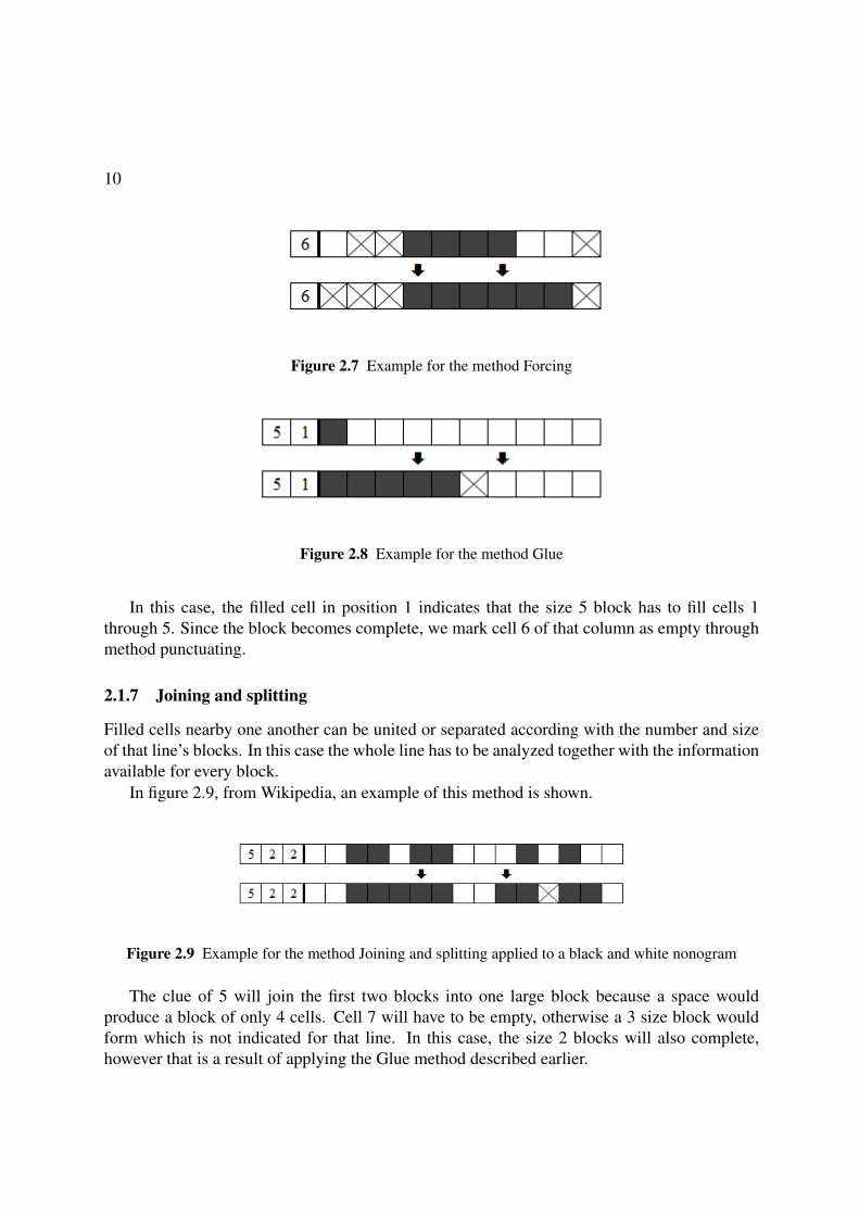
2.1.7 Joining and splitting

Filled cells nearby one another can be united or separated according with the number and sizeof that line’s blocks. In this case the whole line has to be analyzed together with the informationavailable for every block.

In figure 2.9, from Wikipedia, an example of this method is shown.

Figure 2.9 Example for the method Joining and splitting applied to a black and white nonogram

The clue of 5 will join the first two blocks into one large block because a space wouldproduce a block of only 4 cells. Cell 7 will have to be empty, otherwise a 3 size block wouldform which is not indicated for that line. In this case, the size 2 blocks will also complete,however that is a result of applying the Glue method described earlier.

11

Using these methods we can easily solve these more simple puzzles. Figures 2.10(a) through2.11 show the two horizontal iterations and the vertical one made in order to solve the puzzleshown in figure 2.1.

(a) After first horizontal iteration (b) After first vertical iteration

Figure 2.10 Solving a black and white Nonogram Example

2.2 Colored Nonograms

In colored nonograms the clues are composed of pairs that indicate the size and color ofeach sequence of blocks to be filled. For example, the clue <(3,Red), (1,Green), (2,Blue)>indicates that there is a block of 3 contiguous cells of red, followed by a block of one greencell separated or not by a sequence of empty cells, followed by a sequence of two blue cellsseparated or not from the green block by a sequence of empty cells, in that row or column. Thegeneral rule for separating blocks is that if a block is of the same color of the previous one in therespective sequence then they must be separated by at least an empty cell. Otherwise (i.e., thetwo blocks have different colors), they may have no cells in between, i.e., they may be adjoiningblocks. Note that in the particular case of black and white nonograms this means that blocksin a sequence must always be separated by at least one empty cell. Figure 1.2 represents anexample of a colored nonogram with 10 lines by 8 columns with 3 colors.

In the same way as black and white nonograms, in order to solve this kind of puzzle itis necessary to determine which cells will be filled (colored) and which will be empty (white).Determining which cells will be empty is as important as determining which will be filledbecause the former will help delimiting the solutions for the blocks of each line or column.

As referred earlier, black and white nonograms are a special case of colored nonograms (are

12

Figure 2.11 Solving a black and white Nonogram Example — after last (horizontal) iteration

two colored nonograms). In that way, the same methods, with some nuances, can be applied tocolored nonograms, each line at a time, in order to solve them.

These methods are explained again, but now applied to colored nonograms.

2.2.1 Simple boxes

At the beginning of the solution, when there are no filled cells, for each block bi ∈ {b1, ...,bB} ineach row, the space available S (bi) for it is determined, assuming that the remaining blocks aremoved closer to the extremities of the grid as possible (previous blocks to the left and subsequentblock to the right). bi represents a set of filled cells in sequence (vector). The value for S (bi)can be calculated using equation 2.5, where L represents the size of the line, P represents thenumber of pairs of contiguous blocks of the same color on the line and T (bi) represents the sizeof bi.

S (bi) = L−P−B∑

k,i

T (bk) (2.5)

For black and white nonograms equation 2.5 becomes equation 2.1 where B represents thenumber of blocks on the line.

It is also possible to know for each block what is the potential first cell that it can occupythrough equation 2.7, where bi[1] is block’s bi first cell position in the grid and f is a functionthat returns 1 if the blocks are of the same color and 0 otherwise (see equation 2.6 where Cbi isthe color of block i).

f (bi,b j) =

{0 ; Cbi ,Cb j

1 ; Cbi = Cb j(2.6)

13

bi[1] =

{1 ; i = 1bi−1[1] + T (bi−1) + f (bi,bi−1) ; i > 1 (2.7)

For black and white nonograms f always returns 1 and equation 2.7 becomes equation 2.2.Within this set of cells it is possible to determine which subset is actually filled by analyzing

the extremities of the solution, i.e., sliding the block as far to the left as possible and then asfar to the right as possible and checking which cells are common to both solutions. In this way,equation 2.8 gives the size of this sub-block, where T (si) is the size of the sub-block si that canbe determined for block bi.

T (si) = 2T (bi)−S (bi) (2.8)

In the same way, it is possible to obtain the first cell (consequently the remaining) of thissub-block through equation 2.9, where si[1] is the position of the first cell of sub-block si.

si[1] = bi[1] + S (bi)−T (bi) ; T (si) > 0 (2.9)

Figure 2.12 Example 1 for the method Simple boxes

As an example, for the fourth line of the puzzle shown in figure 1.2, L = 8, P = 0, B = 4,T (b1) = 3, T (b2) = 2, T (b3) = 1 and T (b4) = 1. Therefore the space available for the first blockis S (b1) = 8− 0− 4 = 4, S (b2) = 8− 0− 5 = 3, S (b3) = 8− 0− 6 = 2 and S (b4) = 8− 0− 6 = 2.The leftmost indexes each can occupy are b1[1] = 1, b2[1] = 1 + 3 + 0 = 4, b3[1] = 4 + 2 + 0 = 6and b4[1] = 6 + 1 + 0 = 7.

As for the sub-blocks of cells that can be filled at this point, T (s1) = 2× 3− 4 = 2, T (s2) =

2×2−3 = 1, T (s3) = 2×1−2 = 0 and T (s4) = 2×1−2 = 0, i.e., it is not possible to fill, for now,any cell in respect to the third and fourth blocks, but it is possible to fill two cells with respectto the first one and one cell with respect to the second one. It is yet to determine the startingcell of the first and second sub-blocks: s1[1] = 1 + 4−3 = 2 and s2[1] = 4 + 3−2 = 5, i.e., it ispossible to fill, at this point, cells 2, 3 and 5 of that line.

14

2.2.2 Punctuating

In order to solve the puzzle it is also very important to enclose with empty cells the ex-tremities of each completed block that is the same color as the adjacent one, immediately, asdescribed in the method Simple spaces. Precise punctuating usually leads to more Forcing andcan be vital to finishing the puzzle.

Figure 2.13 exemplifies this method for line line 6 of puzzle shown in figure 1.2.

Figure 2.13 Example for the method Punctuating

2.2.3 Simple spaces

The purpose of this method is to find cells that can not be filled by any block due to theconstraints imposed by filled cells. For example, a block that is already complete may have atleast an empty cell to its left and at least another one to its right, unless it is adjacent to thebeginning or the end of the line.

Figure 2.14 from line 2 of the puzzle shown in figure 1.2 shows an example of this method.

Figure 2.14 Example 1 for the method Simple spaces

In figure 2.15, based on one from Wikipedia, a more illustrative example of this method isshown.

First, clue 1 is complete which means that there will be an empty cell to its left and anotherto its right (Punctuating). Then, from clue 3 it is possible to conclude that its block can onlyexpand between the second and the sixth cell because it has to include the fourth cell. Thismeans that cells 1 and 7 will be empty.

15

Figure 2.15 Example 2 for the method Simple spaces

2.2.4 Mercury

Mercury is a special case of Simple spaces. The name comes from the way mercury pullsback from the sides of a container.

If there is a filled cell on a line that is at the same distance from the border as the size of thefirst block, then the first cell has to be empty. This is true because the first block would not fitto the left of the filled cell. It will have to spread through that cell leaving the first cell behind.Besides, when the cell is in reality a set with cells more to the right, there will be more spacesat the beginning of the line, determined by applying this method several times.

In figure 2.16, from line 1 of the puzzle shown in figure 1.2, an example of this method isshown.

Figure 2.16 Example for the method Mercury

2.2.5 Forcing

In this method the importance of empty cells is demonstrated. An empty cell in the middleof an incomplete line can force a block to complete itself to one of the sides of the empty cell.

In figure 2.17, base on the one from Wikipedia, an example of this method is shown.The first block (3) will have to be to the left of the first cell already marked as empty. The

empty one between the two cells already marked as empty cannot belong to any block from thatline which means it has to be empty. Finally, the second block will have to occupy a subset of

16

Figure 2.17 Example for the method Forcing

the last three cells of the line. Applying method Simple boxes to both blocks turns out to fillcells 2, 3 and 9.

2.2.6 Glue

In this method a full cell at the beginning (or the end) of the possible space for a block forcesthe completion of that block to the empty side. In the same way, an empty cell in the middle ofthe possible space for a block can condition the placement of that block’s cells.

In figure 2.18, from column 5 of the puzzle shown in figure 1.2, an example of this methodis shown.

Figure 2.18 Example for the method Glue

In this case, filled brown cell in position 4 preceded by filled green cell in position 3 indicatesthat the size 7 brown block has to fill cells 5 through 10.

2.2.7 Joining and splitting

Filled cells nearby one another can be united or separated according with the number andsize of that line’s blocks. In this case the whole line has to be analyzed together with theinformation available for every block.

In figure 2.19, from column 2 of the puzzle shown in figure 1.2, an example of this methodis shown.

The clue to the size 3 green block will make that the two green cells unite because a spacein cell 3 would divide the first block in two.

17

Figure 2.19 Example for the method Joining and splitting

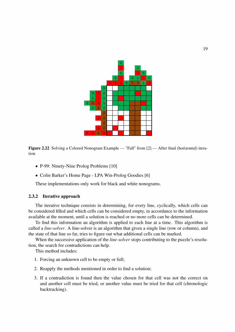
Using these methods one can easily solve these more simple puzzles. Figures 2.20(a)through 2.22 show the three horizontal iterations and the two vertical ones made in order tosolve the puzzle shown in figure 1.2.

(a) After first horizontal iteration (b) After first vertical iteration

Figure 2.20 Solving a Colored Nonogram Example — "Fall" from [2]

2.3 Approaches to solving Nonograms

In the previous section we showed how simpler puzzles can be solved by looking at eachline at a time and applying one or more methods to color cells or mark them as spaces. For morecomplex puzzles we can reach a state where we can not fill more unknown cells by applyingthose methods. At that point we have to try and guess a value (color or space) for a cell and thenreapply the aforementioned methods to try to reach a solution or a contradiction. Eventually

18

(a) After second horizontal iteration (b) After second vertical iteration

Figure 2.21 Solving a Colored Nonogram Example — "Fall" from [2]

we will reach another state where another guess must be made to continue to try to solve thepuzzle, and so on. If a contradiction is reached, then the value we chose for a determined cell iswrong. In black and white puzzles this means that the cell will have the opposite value (emptyif the chosen value was filled, filled otherwise), but in colored nonograms another color can bechosen for that cell. These more complex puzzles are usually difficult to solve by a human.

This is where computer based approaches can be useful.Known approaches for solving nonograms are the depth-first search (brute-force), the it-

erative approach and the ILP approach. A comparison between a genetic algorithm and thedepth-first search algorithm, by Wouter Wiggers [20], was also found. As mentioned in thearticle, the genetic algorithm not always reaches a solution, however it reaches a near solutionvery quickly.

2.3.1 Depth-first search (brute-force)

This approach tries all possible combinations for the set of blocks of each line. For example,for a size 10 line, belonging to a black and white nonogram, with two blocks of sizes 5 and 1,we would have 10 possibilities only for that line, as shown in figure 2.23.

An optimization of this algorithm is to begin with the lines that have fewer possibilities.However, if we want to find all solutions then all possibilities must be explored.

The following are implementations of this approach:

• ECLIPSE program by Joachim Schimpf [14]

19

Figure 2.22 Solving a Colored Nonogram Example — "Fall" from [2] — After final (horizontal) itera-tion

• P-99: Ninety-Nine Prolog Problems [10]

• Colin Barker’s Home Page - LPA Win-Prolog Goodies [6]

These implementations only work for black and white nonograms.

2.3.2 Iterative approach

The iterative technique consists in determining, for every line, cyclically, which cells canbe considered filled and which cells can be considered empty, in accordance to the informationavailable at the moment, until a solution is reached or no more cells can be determined.

To find this information an algorithm is applied to each line at a time. This algorithm iscalled a line-solver. A line-solver is an algorithm that given a single line (row or column), andthe state of that line so far, tries to figure out what additional cells can be marked.

When the successive application of the line-solver stops contributing to the puzzle’s resolu-tion, the search for contradictions can help.

This method includes:

1. Forcing an unknown cell to be empty or full;

2. Reapply the methods mentioned in order to find a solution;

3. If a contradiction is found then the value chosen for that cell was not the correct onand another cell must be tried, or another value must be tried for that cell (chronologicbacktracking).

20

Figure 2.23 Depth-first search — all possibilities for a line

The problem to this method is the choice of a cell to try a contradiction, i.e., having anheuristic to find the best cells to try a value. Besides, while trying a cell for a contradictionanother situation may arise in that another try to find a contradiction must take place, and soforth.

Usually, the best cells to initiate a contradiction try are the following:

• Cells that have many filled neighbors;

• Cells near the border or nearby sets of empty cells;

• Cells that are between lines that consist of more empty cells.

Steven Simpson, in his site [16], describes his algorithm for the resolution of nonograms.As mentioned above, the algorithm tries to solve, or partially solve, a line for each iteration.The order in which lines are tried to be solved is defined by the value of equation 2.10, where Bis the number of blocks of that line, L is the size of the line and T (b1) to T (bB) are the sizes ofeach block. When non-negative, the result is the number of filled cells that can be determinedfrom an empty line. A negative value indicates a shortfall of pre-determined cells. Note thatwhen B = 1 and T (bi) = L then I = L and this is the maximum value.

I = (B+ 1)B∑

i=1

T (bi) + B(B−L−1) (2.10)

Exceptionally, if B = 0 (empty line) then I = L.After a line is chosen a line-solver, or a sequence of line-solvers, are applied to it in order

to fill as many cells as possible. The line-solvers are applied to the line in a predefined rank

21

Table 2.1 Experimental Results (in seconds)

Puzzle R×C×Col NPC Brute-force (Prolog) Brute-force opt (Prolog) Iterative ILPFall 10x8x3 47 1,050.70 0.03 0.07 0.03Fish 16x16x2 164 (timeout) 0.08 0.07 0.21AtoZ 16x16x2 50 (timeout) 0.92 0.10 23.04Time 35x30x5 520 (timeout) (out of memory) 0.21 3.51

order, i.e, higher ranked line-solvers are only applied after lower ranked ones don’t reveal morecells. There are four well-known line-solvers: fast, complete, olsak [13] and fcomp. The firstgets most of the information available; the second gets everything logically deductible, but isvery inefficient; the third is a variation of the first one, but is a little more exhaustive and getsall the information; the fourth is a revised version of the second one, but is significantly moreefficient.

In [23], Jan Wolter compares several nonogram solvers in which the best three (Wolter’spbnsolve [22], Simpson’s nonogram [15] and Olšák’s grid [13]) use one or more of these line-solvers. Simpson’ is the only that does not solve colored nonograms.

2.3.3 Integer Linear Programming approach

Robert A. Bosch [7] presented in 2001 a solution based on Integer Linear Programming aswell as the code that converts the definition of a puzzle in a program that can be used by CPLEX[3] to solve the puzzle.

The mentioned program only works for puzzles that have clues for all the lines.Since this approach only solves black and white nonograms we proposed to develop an ILP

model that solves colored nonograms.The performance results of our approach compared to an adaptation for colored nonograms

of the depth-first search provided by Hett [10], an adapted version of the optimized depth-firstsearch approach also by Hett and Olšák’s grid are shown in table 2.1.

The times were measured on a 2.4 GHz Intel© Centrino© vPro™with 2 GB of RAM runningMicrosoft© Windows©. The Prolog program was run in ECLiPSe [1] and the generated ILPproblems were run on SCIP [4]. Results are shown in table 4.1, where NPC stands for "Numberof Painted Cells". The time limit imposed was 30 minutes.

Given the good performance of the iterative approaches we also proposed to develop a hy-brid model between this approach and the ILP one.

The ILP approach presented here starts from scratch with an empty grid and, in general,could not improve the Iterative method for the available tests, although already presented similarresults using a non commercial tool.

Our initial idea when developing the ILP model, in addition to the new theoretical results,was to use it together with the Iterative method, which we knew was efficient to quickly fill manycells of the grid using simple inferences on the rows and columns clues. That is precisely what

22

we proposed to develop, by applying the ILP model only after the Iterative technique alreadyfilled many cells, thus reducing a lot the model complexity by converting many variables toconstants.

Both Simpson and Wolter have references to other nonogram solvers in [17] and [23], re-spectively.

3 . An ILP model for solving Colored Nonograms

In the previous chapter we verified that no ILP model for solving colored nonograms exists.In this chapter we describe the model we developed for this purpose.

3.1 Model Description

As in [7], our approach is to think of a colored nonogram as a problem comprised of twointerlocking tiling problems: one involving the placement of the row blocks, and the otherinvolving the placement of the column blocks. If a cell is painted (it can be assumed thatunpainted cells are painted white) then it must be covered by both a row block and a columnblock; if it is painted white (not painted) then it must be left uncovered by the row blocks andthe column blocks.

3.1.1 Notation

The notation used here is similar to the one used by Bosch in [7], as follows.

m = the number of rows,

n = the number of columns,

o = the number of colors excluding white (We use a sequence of natural numbers toidentify colors, starting at 1 (1,2, . . . ,o).),

bri = the number of blocks in row i, 1 ≤ i ≤ m,

bcj = the number of blocks in column j, 1 ≤ j ≤ n,

sri,1, s

ri,2, . . . , s

ri,br

i= the block-size sequence for row i,

scj,1, s

cj,2, . . . , s

cj,bc

j= the block-size sequence for column j,

cri,1,c

ri,2, . . . ,c

ri,br

i= the block-color sequence for row i,

ccj,1,c

cj,2, . . . ,c

cj,bc

j= the block-color sequence for column j.

In addition, let

eri,t = the smallest value of j such that row i’s tth block can be placed in row i with its

leftmost pixel occupying cell j,23

24

lri,t = the largest value of j such that row i’s tth block can be placed in row i with itsleftmost pixel occupying cell j,

ecj,t = the smallest value of i such that column j’s tth block can be placed in column j with

its topmost pixel occupying cell i,

lci,t = the largest value of i such that column j’s tth block can be placed in column j withits topmost pixel occupying cell i.

These are constants valid for the empty puzzle. (The letters "e" and "l" stand for "earliest"and "latest"). In our example puzzle, the second row’s first block must be placed so that itsleftmost pixel occupies cell 1 or 2, the second block must be placed so that its leftmost pixeloccupies cell 5 or 6, and the third block must be placed so that its leftmost pixel occupies cell 6or 7. In other words

er2,1 = 1, lr2,1 = 2,er

2,2 = 5, lr2,2 = 6,er2,3 = 6 and lr2,3 = 7.

These values are obtained by iteratively placing the blocks in their leftmost or topmostpossible cells and then placing them in their rightmost or bottommost possible cells. In ourexample, the first block’s first cell is 1 and, since the first block’s size is 4 and the color of bothblocks is different, the second block’s first possible cell is 5. Then, since the color of the thirdblock is also different from the second one and the size of the second block is 1, the third block’sfirst possible cell is 6. Now, the third block is pushed to its rightmost cell (7) and one finds outthat the second block’s last possible cell is 6 and the first block’s last possible cell is 2.

Note that the rules for determining these values are the same for colored or black and whitenonograms. Of course, in black and white puzzles all the blocks are of the same color, whichmeans they have to be separated by at least one empty cell.

3.1.2 Variables

As in the approach by Bosch in [7], in our approach there are three sets of variables. One setspecifies the color of each cell:

∀1≤i≤m,1≤ j≤n zi, j =

c ; if row i’s jth cell is painted

with color c (1 ≤ c ≤ o)

0 ; if row i’s jth cell is notpainted

(3.1)

The other two sets of variables are concerned with placements of the row and column blocks.

∀1≤i≤m,1≤t≤bri ,e

ri,t≤ j≤lri,t

yi,t, j =

1

; if row i’s tth block is placedin row i with its leftmost pixeloccupying cell j

0 ; if not

(3.2)

25

∀1≤ j≤n,1≤t≤bcj,e

cj,t≤i≤lcj,t

x j,t,i =

1

; if column j’s tth block isplaced in column j with itstopmost pixel occupying celli

0 ; if not

(3.3)

3.1.3 Block constraints

To ensure that row i’s tth block appears in row i exactly once, the following imposes

∀1≤i≤m,1≤t≤bri

lri,t∑j=er

i,t

yi,t, j = 1 (3.4)

For line 2 of our example we have

y2,1,1 + y2,1,2 = 1,

y2,2,5 + y2,2,6 = 1,

y2,3,6 + y2,3,7 = 1.

For the next two sets of constraints the auxiliary function (3.5) is defined. This function,which was already defined as equation 2.6 in chapter 1, returns the value 1 if the two argumentsare the same, and 0 otherwise, which will be useful to compare colors of two contiguous blocks.

eq(c1,c2) =

{1 ; if c1 = c20 ; otherwise (3.5)

To ensure that row i’s (t + 1)th block is placed to the right of its tth block, the followingimposes

∀eri,t+1≤ j≤lri,t

yi,t, j ≤

lri,t+1∑j′= j+sr

i,t+eq(cri,t,c

ri,t+1)

yi,t+1, j′ (3.6)

In line 2 of our example we have

y2,1,2 ≤ y2,2,6,

y2,2,6 ≤ y2,3,7.

To ensure that column j’s tth block appears in column j exactly once, the following imposes

26

∀1≤ j≤n,1≤t≤bcj

lcj,t∑i=ec

j,t

x j,t,i = 1 (3.7)

To ensure that column j’s (t + 1)th block is placed under its tth block, the following imposes

∀ecj,t+1≤i≤lcj,t

x j,t,i ≤

lcj,t+1∑i′=i+sc

j,t+eq(ccj,t,c

cj,t+1)

x j,t+1,i′ (3.8)

3.1.4 Double Coverage Constraints

To guarantee that each painted cell is covered by both a row block and a column block, thefollowing pair of sets of inequalities imposes:

∀1≤i≤m,1≤ j≤n zi, j ≤

bri∑

t=1

min{lri,t, j}∑j′=max{er

i,t, j−sri,t+1}

yi,t, j′ × cri,t (3.9)

∀1≤i≤m,1≤ j≤n zi, j ≤

bcj∑

t=1

min{lcj,t,i}∑i′=max{ec

j,t,i−scj,t+1}

x j,t,i′ × ccj,t (3.10)

Without these restrictions the model would allow having cells painted by row blocks, butnot painted by any column block, or vice versa. The first set of inequalities (3.9) states that ifrow i’s jth cell is painted, then at least one of row i’s blocks must be placed in such a way that itcovers row i’s jth cell. (The upper and lower limits of the second summation make sure that j′

satisfies the two pairs of sets of inequalities eri,t ≤ j′ ≤ lri,t and j− sr

i,t + 1 ≤ j′ ≤ j. The first pairholds if, and only if, row i’s tth cell is covered when row i’s tth block is placed in row i with itsleftmost pixel occupying cell j′. The second pair holds if and only if row i’s jth pixel is coveredwhen row i’s tth block is placed in row i with its leftmost pixel occupying pixel j′). The otherset of inequalities (3.10) makes sure that if row i’s jth cell is painted, then at least one of columnj’s blocks covers it. For row 2 of our example we have for cell z2,5 that

z2,5 ≤ y2,1,2× cr2,1 + y2,2,5× cr

2,2,

z2,5 ≤ x5,1,1× cc5,1 + x5,1,2× cc

5,1

If z2,5 is painted, the right hand terms of these inequalities will yield exactly its color valuein a solved puzzle. Otherwise (empty cell), the terms hold value 0. Ideally, the model shouldexpress this disjunction directly, allowing only those 2 values. However, in order to allow ILP

27

solving, it is kept as a linear inequality. Nevertheless, below it is proven that this is sufficientfor a correct and complete model, in the presence of the other sets of constraints.

Finally, constraints that prevent unpainted cells from being covered by the row blocks orcolumn blocks are included — sets of inequalities (3.11) and (3.12).

∀1≤i≤m, 1≤ j≤n, 1≤t≤bri , j−sr

i,t+1≤ j′≤ j, eri,t≤ j′≤lri,t

zi, j ≥ yi,t, j′ × cri,t (3.11)

∀1≤i≤m, 1≤ j≤n, 1≤t≤bcj, ec

j,t≤i′≤lcj,t, i−scj,t+1≤i′≤i zi, j ≥ x j,t,i′ × cc

j,t (3.12)

In line 2 of our example we have

z2,5 ≥ y2,1,2× cr2,1, z2,5 ≥ y2,2,5× cr

2,2,

z2,5 ≥ x5,1,1× cc5,1, z2,5 ≥ x5,1,2× cc

5,1.

One might think that it is necessary to ensure that each painted cell must be covered by onerow block and one column block of the same color. However, the remaining sets of constraintsensure that there is only the need to guarantee that a painted cell must be covered by one rowblock and one column block. In order to prove it, let us explore all the possibilities regardingthe coverage of some cell z:

1. No block covers cell z;

2. Only one block covers cell z and it is of the same color;

3. Only one block covers cell z and its color is smaller than the color of z;

4. Only one block covers cell z and its color is greater than the color of z;

5. More than one block covers cell z;

Of these five possibilities, only the first two are possible in real puzzles. The last three arethe ones that our model has to avoid.

In sake of simplicity, but with no loss of generality, only inequality (3.9), for lines, of thedouble coverage constraints will be used in our case analysis for these five possibilities:

Possibility 1: The only way to satisfy this possibility is with an empty cell z, with value 0,which, by inequality (3.9), will guarantee that no block covers it (forcing the respective yi,t, j′

variables to be 0), i.e.

bri∑

t=1

Max{lri,t, j}∑j′=Min{er

i,t, j−sri,t+1}

yi,t, j′ × cri,t = 0.

28

Possibility 2: This possibility fully satisfies inequality (3.9), corresponding to the equality ofboth terms.

Possibility 3: If a single block of smaller color than the color of cell z covers it then inequality(3.9) is not satisfied, thus disallowing such possibility, as desired.

Possibility 4: In the case that there may be one block that covers cell z, and which color isgreater than the color of z, then inequality (3.9) would be satisfied. However, this would violateinequality (3.11) thus turning the solution invalid.

Possibility 5: If more than one block covers cell z, the set of inequalities (3.9) could only besatisfied if the sum of the colors of the covering blocks is greater than or equal to the color ofcell z. But this would violate the set of equations (3.4) thus turning the solution invalid.

3.1.5 Objective Function

Since this is a satisfaction problem there is no need for an objective function, but since ILPsolvers need one, the following is included (note that this function is a constant and we alreadyknow its value):

minimize/maximizem∑

i=1

n∑j=1

zi, j (3.13)

3.1.6 Pre-conditions

We also include in our approach one pre-condition in order to verify whether the puzzle istrivially impossible to solve, before even trying to search for a solution (another improvementwith respect to [7]). This is a necessary, but not sufficient condition that will save the time oftrying to solve a puzzle that is impossible, and that also helps determining whether there is anyerror in the definition of the puzzle. This condition, shown by equation (3.14), checks whetherthe sum of the sizes of all blocks of each color is the same for both the rows and columns clues.

∀c∈{1,...,o}

m∑i=1

bri∑

t=1

f (sri,t,c

ri,t,c) =

n∑j=1

bcj∑

t=1

f (scj,t,c

cj,t,c) (3.14)

where f (s,c1,c2) = s if c1 = c2, and 0 otherwise.

29

3.2 Instantiation to Black and White Nonograms

If o is set to 1 (o = 1), thus allowing only black and white in a puzzle, our model becomes theone provided by Bosch in [7], i.e., definition (3.1) becomes

zi, j =

{1 ; if row i’s jth cell is painted0 ; if row i’s jth cell is not painted

(3.15)

Definitions (3.2) and (3.3) are kept from the approach provided by Bosch. Equation (3.4)is equal to the one in the approach by Bosch, but inequality (3.6) was extended so block t + 1can follow block t immediately, due to possible contiguous blocks of different colors. For blackand white puzzles it corresponds exactly to the formulation in [7] since all blocks have the samecolor which leads the eq function to always yield value 1. Inequalities (3.7) and (3.8) are similar,but regard columns. Finally, since the only possible color takes value 1, the double coverageconstraints set by the sets of inequalities (3.9) and (3.10) become

∀1≤i≤m,1≤ j≤n zi, j ≤

bri∑

t=1

min{lri,t, j}∑j′=max{er

i,t, j−sri,t+1}

yi,t, j′ , (3.16)

∀1≤i≤m,1≤ j≤n zi, j ≤

bcj∑

t=1

min{lcj,t,i}∑i′=max{ec

j,t,i−scj,t+1}

x j,t,i′ , (3.17)

∀1≤i≤m,1≤ j≤n,1≤t≤bri , j−sr

i,t+1≤ j′≤ j,eri,t≤ j′≤lri,t

zi, j ≥ yi,t, j′ (3.18)

and

∀1≤i≤m,1≤ j≤n,1≤t≤bcj,e

cj,t≤i′≤lcj,t,i−sc

j,t+1≤i′≤i zi, j ≥ x j,t,i′ (3.19)

as in [7] (where the min and max functions are incorrectly swapped in the summation limits).

3.3 Finding Multiple Solutions

The described ILP model allows finding a single solution to a puzzle, which actually is the bestone, although in this case all solutions are alike since the optimizing function is a constant.

Nonograms are satisfaction problems, which in ILP must be modeled as optimization prob-lems. Since it is possible that the obtained solution is not unique, we also try to find additionalsolutions to a puzzle. For that, the algorithm developed by Jung-Fa Tsai et al. described in [18]was first considered. This algorithm uses an integer cut to exclude the previously found solu-tion, extending the ILP model to a Mixed ILP model (MILP), which is the general approach tofinding additional solutions in ILP. But, in fact, a much simpler approach was used by applyinga binary cut similar to the one proposed by Balas and Jeroslow in [5].

30

Since our binary variables (either yi,t, j or x j,t,i) are enough to provide the solution (theycompletely determine the filled puzzle, since clues are constant), a binary cut is enough.

The cut that needed to be applied to exclude an existing solution is shown in (3.20) usingthe y set of variables (the x set of variables could also be used).

∑(i,t, j)∈A

yi,t, j−∑

(i,t, j)∈B

yi,t, j ≤ |A| −1,A = {(i, t, j) | yi,t, j = 1},B = {(i, t, j) | yi,t, j = 0} (3.20)

Basically, after finding a solution to the problem, the constraints in inequality (3.20) areadded to the problem and another try is made to find another solution.

3.4 Hybrid model

The hybrid model we propose here basically consists in substituting the search part of the iter-ative approach by our ILP model.

At first, the puzzle is logically solved, i.e., one or more line-solvers are applied to every lineof the puzzle, repeatedly, until there is no more information that can be inferred. Then, if thepuzzle is not completely solved, the ILP model is instantiated.

Our implementation generates a CPLEX LP file (.lp) that represents the current state of thepuzzle according to the model presented in section 3.1. This approach is more flexible thangenerating the ILP model specifically for a solver like SCIP [4] or CPLEX [3] because it allowsthe comparison of results between different ILP solvers.

SCIP is currently one of the fastests non-commercial mixed integer programming (MIP)solvers. ILOG CPLEX©is a commercial mathematical programming optimizer that, amongother things, solves mixed integer programs. Although SCIP is advertised as the best performingnon-commercial MIP solver, CPLEX — the best MIP solver — is five times faster.

The process of instantiating our ILP model, and subsequently generating the LP file, en-volves the following steps:

• Compute earliest and latest constants

• Write objective function to file

• Write block constraints to file

• Write double coverage constraints to file

• Write bounds to file: here is where the partial solution found by the iterative approach isinserted in the ILP model

• Write all the variables to file

31

Since among the best performing implementations of the iterative approach only pbnsolveand Olšák’s (grid) can solve colored nonograms, we decided to adapt pbnsolve into our hybridapproach. The reason we did not choose grid was that the program code comments are inCzech. On the other hand, pbnsolve’s code comments are very complete and understandable.Steven Simpson’s nonogram [16] can not solve colored nonograms.

Also, for testing purposes, we did not implement Balas and Jeroslow’s binary cut in thisapproach.

4 . Results

In the previous chapter our ILP model for solving colored nonograms was described. Wealso described an hybrid approach to solving colored nonograms between the iterative and theILP ones.

Here, we present the results of the performance tests we ran in order to compare the differentapproaches to solving colored nonograms.

First we present the results between our pure ILP approach and the iterative and the depth-first search ones. Then we show the results obtained by comparing our hybrid approach and theiterative one.

4.1 Pure ILP approach

In order to test the performance of the model described in Chapter 3 (without the use ofBalas and Jeroslow’s cut) it was tested against three algorithms: one adaptation (the originalprogram solves only black and white nonograms) of an implementation in Prolog of a bruteforce search by Werner Hett [10], an optimized variant of this implementation (by altering theordering of the line tasks) and an implementation in C of the iterative approach by Mirek Olšákand Petr Olšák available in [13].

Four puzzles were used for the purpose of these tests: the "Fall" puzzle from Griddlers.net[2] (10x8x3, i.e. a 10 by 8 grid with 3 colors) used as an example in this dissertation (figure1.2), the "Fish" and the "AtoZ" puzzles (16x16x2) from Ali Corbin’s web page [8], and the"Time" adapted from the copyrighted Sunday Telegraph & Aenigma Design and colored byBrian Grainger (35x30x5) [9].

The times were measured on a 2.4 GHz Intel® Centrino® vPro™with 2 GB of RAM runningMicrosoft® Windows®. The Prolog program was run in ECLiPSe [1] and the generated ILPproblems were run on SCIP [4]. Results are shown in table 4.1, where NPC stands for "Numberof Painted Cells". The time limit imposed was 30 minutes.

As shown in table 4.1 the first puzzle was solved almost instantly by both the iterativeimplementation and the ILP approach. The brute-force implementation took about 17 minutesto return the results. With some optimization applied to the brute-force approach, namely by

Table 4.1 Experimental Results (in seconds)

Puzzle R×C×Col NPC Brute-force (Prolog) Brute-force opt (Prolog) Iterative ILPFall 10x8x3 47 1,050.70 0.03 0.07 0.03Fish 16x16x2 164 (timeout) 0.08 0.07 0.21AtoZ 16x16x2 50 (timeout) 0.92 0.10 23.04Time 35x30x5 520 (timeout) (out of memory) 0.21 3.51

33

34

Table 4.2 Results of adding equation (4.1) to ILP (in seconds)

Puzzle ILP ILP w/ ACFall 0.03 0.03Fish 0.21 0.11AtoZ 23.04 33.58Time 3.51 2.45

re-sorting the line tasks, the puzzle is also solved almost instantly. The "Fish" puzzle is a littleharder to solve. The brute-force approach was not able to solve it in a timely fashion (within30 minutes) although all other approaches solved it pretty quickly. The other 16x16 puzzle —"AtoZ" — is even harder to solve. This was the hardest puzzle to solve by the ILP approach.The fourth (and biggest) puzzle could not be solved by the brute-force algorithms. The iterativeapproach found all 14 solutions to the puzzle in less than half a second and the ILP approachtook about 3.5 seconds to find the first one.

In order to try to improve the results of the ILP approach we added equation (4.1) to the setof constraints, where the right-hand term is a constant.

m∑i=1

n∑j=1

zi, j =

m∑i=1

bri∑

t=1

sri,t × cr

i,t (4.1)

We believed that by adding this constraint, the solver would reach a solution sooner sincethe objective value for the problem was already defined (is a constant).

The results are shown in table 4.2, where AC means "Additional Constraint".Only the performance on the hardest puzzle was not improved which turns out to be incon-

clusive as to the advantages of adding this extra constraint.

4.2 Nonogram Generator

In order to test the different approaches in a proper manner a set of a substantial number ofpuzzles with varying dimensions, number of colors and densities should be used. To accomplishthis we decided to create a nonogram puzzle generator.

By developing this generator we also solved the problem of converting the puzzles to thedifferent file formats supported by each approach.

This generator allows the generation of puzzles based on number of rows, number of columns,number of colors, global density (amount of painted cells vs. available cells — number of rows× number of columns) and density by color. The puzzles are generated by painting randomlychosen cells with specific or randomly chosen colors and then obtaining the clues from the grid.The generated puzzle can then be saved as a Bosch based file format (adapted for colored nono-grams), an Olšák file format or a Hett [10] list based Prolog format (also adapted for colored

35

nonograms).Examples of the file formats created by our generator for puzzle shown in figure 4.1 are

shown in appendix D.

Figure 4.1 Generated nonogram

Bosch’s based file format begins with a puzzle definition section where the dimension ofthe puzzle and the its number of colors are defined (excluding the background color). We alsoadded a title field in order to identify the puzzle more easily:

title: TEST_20x20x5_101number_of_rows: 20number_of_columns: 20number_of_colors: 5

After the puzzle definition section follows the clues for the rows. Here, the number ofclusters is defined for each row and after, the blocks’ sizes and colors are defined:

row_1:number_of_clusters: 3size(s): 1 1 1color(s): 1 1 1

36

The last section of the file defines the clues for the columns and its format is similar to theprevious one.

In Olšák’s file format all text before "#" or ":" in the first column is ignored. If the puzzlehas colored blocks then we need to write "#D" or "#d" in the first column.

This line denotes the start of the color declaration. The color declaration ends by a ":" in thefirst column and the block declarations follow at the next line immediately.

Lines of color declarations have the following format:<spaces><inchar><colon><outchar><spaces><word_XPM><spaces><comment>The < spaces> denotes zero or more spaces or tabs. The exception: <word_XPM> has to

be terminated by one or more spaces and/or tabs.<inchar> is a character used to identify a color in the block declaration section, after the

numbers that represent their sizes. digits, spaces, commas or tab can not be used for <inchar>declaration. The "0" and "1" are exceptions, see bellow.<outchar> is a character which will be used to represent that color in the terminal printing

of the solution.<word_XPM> is the word (without spaces) used in XPM format for color declaration. we

can use the natural word for the color (e.g. blue) or a six hexadecimal digits preceded by a "#"that represents a RGB color (e.g. "#0000FF"). In order to use a natural word for colors theyhave to be defined in the rgb.txt of the X window system where program runs.

If <inchar> is "0", then this line declares the color for the background of the image. If thisdeclaration is omitted white will be used as the background color.

If <inchar> is "1", then this line declares the "default" color of blocks. This color is usedif no <inchar> follows the block declaration. If this line is omitted then the color must bespecified for each block declaration.

Each block declaration section (one for row and one for columns) begins after a line with acolon. For every line of the puzzle a sequence of size and color pairs (without spaces separatingthe size and the color) separated by spaces or tabs.

Hett’s based file format is defined as a predicate with three arguments: a title and two lists.Each list defines the list of blocks for rows and columns and is composed of a list of blocks thatcan be empty. Each block is another list with two elements: a size and a color.

4.3 Hybrid ILP approach

For the purpose of this work 270 problems were generated divided in three large subsetsof 20×20×5 (number of rows by number of columns with number of colors), 40×60×5 and100×100×5. Each of these subsets contains 90 problems divided by density (10 of each density— 10%, 20%, 30%, 40%, 50%, 60%, 70%, 80% and 90%).

This hybrid ILP solution was tested against pbnsolve — the implementation in C of theiterative approach by Jan Wolter available in [22]. Due to the poor results shown by the Prologimplementations by Werner Hett [10] they were removed from this test.

37

We imposed a time limit of 15 minutes for solving each of the puzzles in both approaches.The results were not the ones we expected. The iterative approach is still the fastest to

solve colored nonograms and was the one that solved more nonograms within the 15 minutestimeframe we imposed. Also, in terms of memory consumption, the iterative approach is better.Although the save and load times of the .lp files generated from our sample set of nonogramswere not taken into account, some were over 100 MB in size. This means that if these timeswere added the results would be worse. Of course, if these times were taken into account wewould be penalizing the ILP model with hard disk access (much slower than memory access).A solution to this problem would be to completely integrate the hybrid approach, i.e., withoutgenerating any files.

In table 4.3 the number of puzzles solved by each approach and by dimension is shown.Note that if the puzzle is logically solvable it does not count to either the ILP or the iterativeapproaches.

Table 4.3 Number of solved puzzles by method and dimension

100x100 40x60 20x20 TotalLogically solvable 0 4 22 26Iterative with search 50 61 68 179ILP 42 46 68 156

In table 4.4 the number of puzzles solved by each approach, by dimension and by puzzledensity is shown. The letters "S", "M", and "L" stand for small (20x20), medium (40x60) andlarge (100x100), respectivelly. Again, if the puzzle is logically solvable it does not count to anyother approach.

Table 4.4 Number of solved puzzles by method, dimension and density

10% 20% 30% 40% 50% 60% 70% 80% 90% Total

Logically solvableS 1 5 6 3 15M 1 10 11L

Iterative with searchS 10 10 10 10 10 9 5 4 68M 8 2 5 10 10 10 9 7 61L 10 10 10 10 50

ILPS 10 10 10 10 10 9 5 4 68M 10 10 10 9 7 46L 2 10 10 10 42

In table 4.5 the number of puzzles solved by each approach and by puzzle density is shown.Again, if the puzzle is logically solvable it does not count to any other approach.

38

Table 4.5 Number of solved puzzles by method and density

10% 20% 30% 40% 50% 60% 70% 80% 90% TotalLogically solvable 1 5 7 13 26Iterative with search 18 12 10 15 30 29 25 23 17 179ILP 10 10 10 10 22 29 25 23 17 156

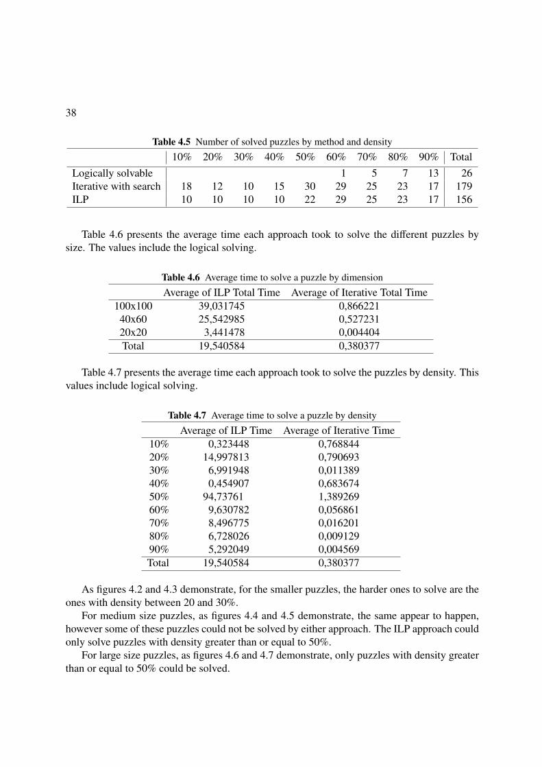
Table 4.6 presents the average time each approach took to solve the different puzzles bysize. The values include the logical solving.

Table 4.6 Average time to solve a puzzle by dimension

Average of ILP Total Time Average of Iterative Total Time100x100 39,031745 0,866221

40x60 25,542985 0,52723120x20 3,441478 0,004404Total 19,540584 0,380377

Table 4.7 presents the average time each approach took to solve the puzzles by density. Thisvalues include logical solving.

Table 4.7 Average time to solve a puzzle by density

Average of ILP Time Average of Iterative Time10% 0,323448 0,76884420% 14,997813 0,79069330% 6,991948 0,01138940% 0,454907 0,68367450% 94,73761 1,38926960% 9,630782 0,05686170% 8,496775 0,01620180% 6,728026 0,00912990% 5,292049 0,004569Total 19,540584 0,380377

As figures 4.2 and 4.3 demonstrate, for the smaller puzzles, the harder ones to solve are theones with density between 20 and 30%.

For medium size puzzles, as figures 4.4 and 4.5 demonstrate, the same appear to happen,however some of these puzzles could not be solved by either approach. The ILP approach couldonly solve puzzles with density greater than or equal to 50%.

For large size puzzles, as figures 4.6 and 4.7 demonstrate, only puzzles with density greaterthan or equal to 50% could be solved.

39

0

3,75

7,5

11,25

15

10% 20% 30% 40% 50% 60% 70% 80%0

2,5

5

7,5

10

ILP :: Average resolution time by density (20x20) Number of solved puzzles

Figure 4.2 ILP: Average resolution by density (20x20) and number of solved puzzles

0

0,005

0,01

0,015

0,02

10% 20% 30% 40% 50% 60% 70% 80%0

2,5

5

7,5

10

Iterative :: Average resolution time by density (20x20) Number of solved puzzles

Figure 4.3 Iterative: Average resolution by density (20x20) and number of solved puzzles

We could also analize the average resolution time by block density. As figures B.1, B.2,B.3, B.4, B.5 and B.6 in Appendix B demonstrate, the results vary in a similar way to the onesby puzzle density.

It seems clear that the puzzles with density between 20 and 30% are harder to solve, spe-cially if their size is large. In fact, when there are few cells to fill in the grid (but not to few) itbecomes harder to logically solve the puzzle. This means that the puzzle is solved largely bysearch with backtracking, in case of the iterative approach, or by applying our pure ILP model.In either case the process is computationally heavy.

Full results of these tests can be found in table A.1 in Appendix A. The times are presentedin seconds and were obtained on a 1.8 GHz Intel® Pentium® M with 1 GB of RAM. Thegenerated ILP problems were run on SCIP [4].

40

0

37,5

75

112,5

150

10% 20% 30% 40% 50% 60% 70% 80% 90%0

2,5

5

7,5

10

ILP :: Average resolution time by density (40x60) Number of solved puzzles

Figure 4.4 ILP: Average resolution by density (40x60) and number of solved puzzles

It was also possible to test the addition of a constraint equal to the objective function on asubset of our set of puzzles (only small and medium size puzzles). Since we know the value ofthe objective function in advance, we added the corresponding constraint to the other constraintsin the ILP problem. The results obtained by adding this constraint were generally worse, as thacharts and the table in Appendix C demonstrate.

Finally, we compared the results obtained by the pure ILP approach with the ones obtainedby the hybrid one, on the smaller puzzles. The hybrid approach performed better, as Figure 4.8demonstrates.

We could also test our hybrid approach with CPLEX on a 3.0 GHz Intel® Core™Duo ma-chine with 2 GB of RAM and although we could not analyze them in detail, the results weresignificantly better than the results we obtained with SCIP. Four puzzles that could not be solvedby SCIP within the 15 minutes window were solved by CPLEX and some puzzles were solvedseven times (and more) faster than with SCIP.

41

0

1,25

2,5

3,75

5

10% 20% 30% 40% 50% 60% 70% 80% 90%0

2,5

5

7,5

10

Iterative :: Average resolution time by density (40x60) Number of solved puzzles

Figure 4.5 Iterative: Average resolution by density (40x60) and number of solved puzzles

0

125

250

375

500

50% 60% 70% 80% 90%0

2,5

5

7,5

10

ILP :: Average resolution time by density (100x100) Number of solved puzzles

Figure 4.6 ILP: Average resolution by density (100x100) and number of solved puzzles

42

0

1,25

2,5

3,75

5

50% 60% 70% 80% 90%0

2,5

5

7,5

10

Iterative :: Average resolution time by density (100x100) Number of solved puzzles

Figure 4.7 Iterative: Average resolution by density (100x100) and number of solved puzzles

43

0

175

350

525

700

Hybrid ILP vs. Pure ILP comparison (20x20)

Hybrid ILP Pure ILP

Figure 4.8 Hybrid ILP vs. Pure ILP comparison (20x20)

5 . Conclusions and Future Work

In this dissertation we presented a new ILP approach to model the Colored Nonogramsproblem, which generalizes a known approach which was limited to black and white Nono-grams. We demonstrated its correctness and, additionally, we also showed how to efficientlyfind possible additional solutions by a simple adaptation of a known technique using a binarycut, by taking advantage of the specificities of this problem. This work developed during thisMaster led to the publication of the article [12].

We also enhanced the aforementioned model by merging it with an iterative approach thusproviding an hybrid approach to colored nonograms.

In order to provide a significant sample set of puzzles, for test and comparisons, we alsodeveloped a nonogram generator. This generator allows us to create puzzles given their width,height, color count and density (either global or by color) and then to save them in three formats:Bosch’s variant for colored nonograms, Olšák’s format and a Hett [10] list based Prolog formatvariant for colored nonograms.

The hybrid model results were not the ones we expected. The iterative approach is still thefastest to solve colored nonograms and was the one that solved more nonograms within the 15minutes timeframe we imposed. Also, in terms of memory consumption, the iterative approachis better. Some of the .lp files generated from our largest sample nonograms were over 100 MBin size which is a consequence of the great amount of variables and constraints that consume alot of memory.

This also means that maybe there is room for improvement. First by fully integrating themodel in one tool and then by trying to fine tune the model. One example of this can be tochange the objective function and include the objective function value as a constraint and useCPLEX to verify the results. Specially for the more complex puzzles that were not solved byeither approach, within the 15 minutes window we defined.

Another way the model can be improved is by trying to implement a backtracking mecha-nism with ILP, i.e, instead of trying to find a final solution with the ILP model, we try to find apartial solution and then reapply the iterative approach to the partial solution.

The model can also be improved in order to solve other problems, like triddlers.The nonogram puzzle generator developed can also be improved by allowing to take into

account the number of blocks of a puzzle. With the current approach, the puzzles generatedhave often a large number of small size blocks.

45

A . Full Results

47

48

Tabl

eA

.1:F

ullR

esul

ts(i

nse

cond

s)

Title

WH

CD

ens.

H Blk

sV B

lks

Cel

lslo

gi-

cally

solv

ed

Cel

lsIL

Pst

ate

Log

ictim

eIL

PTo

tal

Tim

eIt

erat

ive

Tota

lTi

me

TE

ST_1

00x1

00x5

_101

100

100

510

%90

991

411

3710

000

ILP

unso

lved

0,07

1626

(tim

eout

)(t

imeo

ut)

TE

ST_1

00x1

00x5

_101

100

100

510

%90

991

411

3710

000

ILP

unso

lved

0,07

236

(tim

eout

)(t

imeo

ut)

TE

ST_1

00x1

00x5

_102

100

100

510

%90

892

010

1610

000

ILP

unso

lved

0,07

13(t

imeo

ut)

(tim

eout

)T

EST

_100

x100

x5_1

0310

010

05

10%

904

920

1209

1000

0IL

Pun

solv

ed0,

0644

72(t

imeo

ut)

(tim

eout

)T

EST

_100

x100

x5_1

0410

010

05

10%

915

904

1330

1000

0IL

Pun

solv

ed0,

0359

93(t

imeo

ut)

(tim

eout

)T

EST

_100

x100

x5_1

0510

010

05

10%

892

899

1512

1000

0IL

Pun

solv

ed0,

0652

62(t

imeo

ut)

(tim

eout

)T

EST

_100

x100

x5_1

0610

010

05

10%

929

906

1190

1000

0IL

Pun

solv

ed0,

0725

68(t

imeo

ut)

(tim

eout

)T

EST

_100

x100

x5_1

0710

010

05

10%

913

899

1527

1000

0IL

Pun

solv

ed0,

0348

74(t

imeo

ut)

(tim

eout

)T

EST

_100

x100

x5_1

0810

010

05

10%

918

899

1227

1000

0IL

Pun

solv

ed0,

0671

37(t

imeo

ut)

(tim

eout

)T

EST

_100

x100

x5_1

0910

010

05

10%

899

918

1041

1000

0IL

Pun

solv

ed0,

0724

05(t

imeo

ut)

(tim

eout

)T

EST

_100

x100

x5_1

1010

010

05

10%

921

905

1075

1000

0IL

Pun

solv

ed0,

0675

14(t

imeo

ut)

(tim

eout

)T

EST

_100

x100

x5_2

0110

010

05

20%

1670

1674

257

1000

0IL

Pun

solv

ed0,

0852

34(t

imeo

ut)

(tim

eout

)T

EST

_100

x100

x5_2

0210

010

05

20%

1648

1685

155

1000

0IL

Pun

solv

ed0,

0835

76(t

imeo

ut)

(tim

eout

)T

EST

_100

x100

x5_2

0310

010

05

20%

1670

1691

209

1000

0IL

Pun

solv

ed0,

0820

54(t

imeo

ut)

(tim

eout

)T

EST

_100

x100

x5_2

0410

010

05

20%

1674

1642

172

1000

0IL

Pun

solv

ed0,

0845

22(t

imeo

ut)

(tim

eout

)T

EST

_100

x100

x5_2

0510

010

05

20%

1666

1680

221

1000

0IL

Pun

solv

ed0,

0789

25(t

imeo

ut)

(tim

eout

)T

EST

_100

x100

x5_2

0610

010

05

20%

1704

1686

145

1000

0IL

Pun

solv

ed0,

0917

08(t

imeo

ut)

(tim

eout

)T

EST

_100

x100

x5_2

0710

010

05

20%

1673

1694

126

1000

0IL

Pun

solv

ed0,

0885

52(t

imeo

ut)

(tim

eout

)T

EST

_100

x100

x5_2

0810

010

05

20%

1678

1707

226

1000

0IL

Pun

solv

ed0,

0822

45(t

imeo

ut)

(tim

eout

)T

EST

_100

x100

x5_2

0910

010

05

20%

1684

1681

279

1000

0IL

Pun

solv

ed0,

0798

66(t

imeo

ut)

(tim

eout

)T

EST

_100

x100

x5_2

1010

010

05

20%

1649

1681

219

1000

0IL

Pun

solv

ed0,

0842

09(t

imeo

ut)

(tim

eout

)T

EST

_100

x100

x5_3

0110

010

05

30%

2278

2359

191

1000

0IL

Pun

solv

ed0,

0848

82(t

imeo

ut)

(tim

eout

)T

EST

_100

x100

x5_3

0210

010

05

30%

2318

2350

200

1000

0IL

Pun

solv

ed0,

1195

61(t

imeo

ut)

(tim

eout

)T

EST

_100

x100

x5_3

0310

010

05

30%

2306

2333

194

1000

0IL

Pun

solv

ed0,

0871

55(t

imeo

ut)

(tim

eout

)T

EST

_100

x100

x5_3

0410

010

05

30%

2344

2329

209

1000

0IL

Pun

solv

ed0,

0870

33(t

imeo

ut)

(tim

eout

)T

EST

_100

x100

x5_3

0510

010

05

30%

2298

2319

197

1000

0IL

Pun

solv

ed0,

0896

(tim

eout

)(t

imeo

ut)

TE

ST_1

00x1

00x5

_306

100

100

530

%22

9123

2418

110

000

ILP

unso

lved

0,08

9485

(tim

eout

)(t

imeo

ut)

TE

ST_1

00x1

00x5

_307

100

100

530

%22

6822

8820

810

000

ILP

unso

lved

0,08

648

(tim

eout

)(t

imeo

ut)

TE

ST_1

00x1

00x5

_308

100

100

530

%22

7923

7224

910

000

ILP

unso

lved

0,08

8873

(tim

eout

)(t

imeo

ut)

TE

ST_1

00x1

00x5

_309

100

100

530

%23

1723

4214

410

000

ILP

unso

lved

0,12

6233

(tim

eout

)(t

imeo

ut)

Con

tinue

don

Nex

tPag

e...

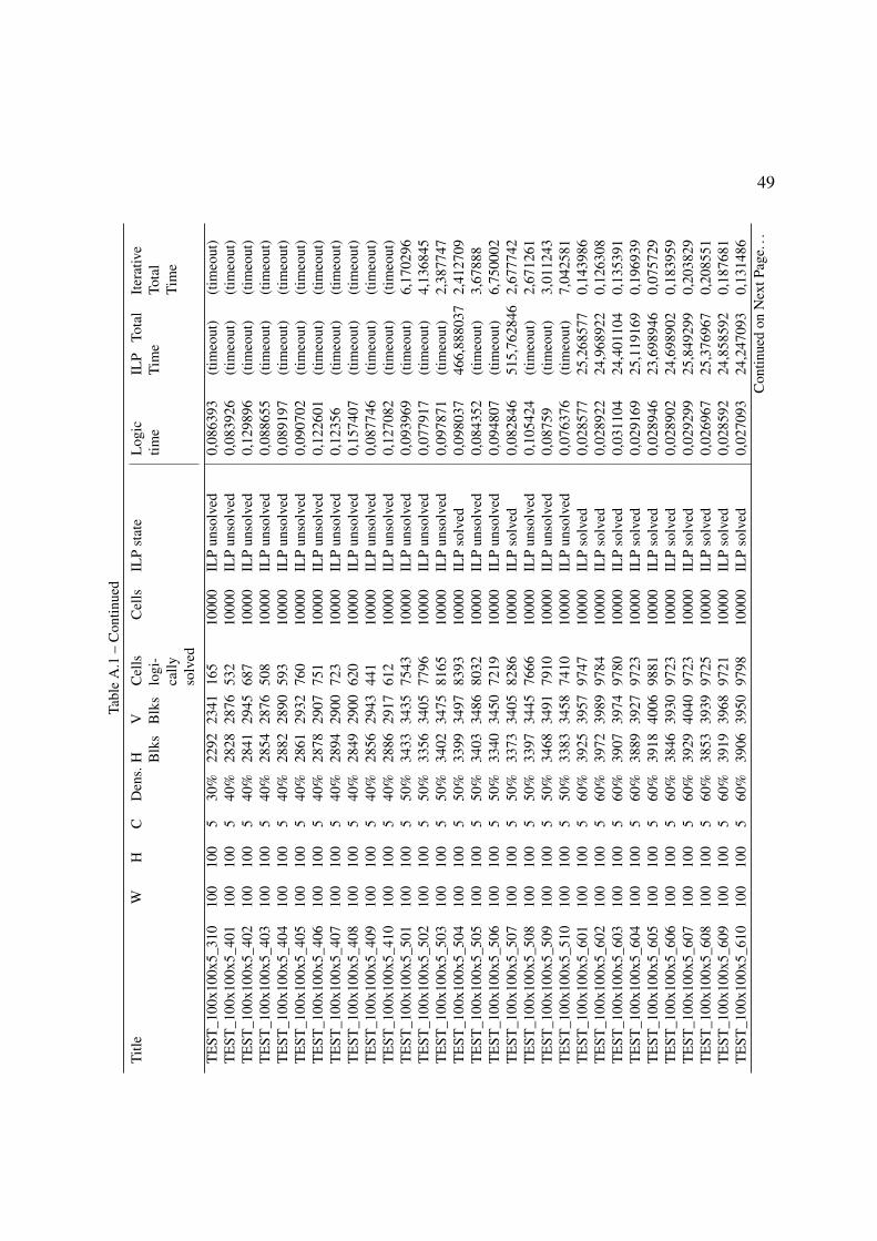
49

Tabl

eA

.1–

Con

tinue

d

Title

WH

CD

ens.

H Blk

sV B

lks

Cel

lslo

gi-

cally

solv

ed

Cel

lsIL

Pst

ate

Log

ictim

eIL

PTo

tal

Tim

eIt

erat

ive

Tota

lTi

me

TE

ST_1

00x1

00x5

_310

100

100

530

%22

9223

4116

510

000

ILP

unso

lved

0,08

6393

(tim

eout

)(t

imeo

ut)

TE

ST_1

00x1

00x5

_401

100

100

540

%28

2828

7653

210

000

ILP

unso

lved

0,08

3926

(tim

eout

)(t

imeo

ut)

TE

ST_1

00x1

00x5

_402

100

100

540

%28

4129

4568

710

000

ILP

unso

lved

0,12

9896

(tim

eout

)(t

imeo

ut)

TE

ST_1

00x1

00x5

_403

100

100

540

%28

5428

7650

810

000

ILP

unso

lved

0,08

8655

(tim

eout

)(t

imeo

ut)

TE

ST_1

00x1

00x5

_404

100

100

540

%28

8228

9059

310

000

ILP

unso

lved

0,08

9197

(tim

eout

)(t

imeo

ut)

TE

ST_1

00x1

00x5

_405

100

100

540

%28

6129

3276

010

000

ILP

unso

lved

0,09

0702

(tim

eout

)(t

imeo

ut)

TE

ST_1

00x1

00x5

_406

100

100

540

%28

7829

0775

110

000

ILP

unso

lved

0,12

2601

(tim

eout

)(t

imeo

ut)

TE

ST_1

00x1

00x5

_407

100

100

540

%28

9429

0072

310

000

ILP

unso

lved

0,12

356

(tim

eout

)(t

imeo

ut)

TE

ST_1

00x1

00x5

_408

100

100

540

%28

4929

0062

010

000

ILP

unso

lved

0,15

7407

(tim

eout

)(t

imeo

ut)

TE

ST_1

00x1

00x5

_409

100

100

540

%28

5629

4344

110

000

ILP

unso

lved

0,08

7746

(tim

eout

)(t

imeo

ut)

TE

ST_1

00x1

00x5

_410

100

100

540

%28

8629

1761

210

000

ILP

unso

lved

0,12

7082

(tim

eout

)(t

imeo

ut)

TE

ST_1

00x1

00x5

_501

100

100

550

%34

3334

3575

4310

000

ILP

unso

lved

0,09

3969

(tim

eout

)6,

1702

96T

EST

_100

x100

x5_5

0210

010

05

50%

3356

3405

7796

1000

0IL

Pun

solv

ed0,

0779

17(t

imeo

ut)

4,13

6845

TE

ST_1

00x1

00x5

_503

100

100

550

%34

0234

7581

6510

000

ILP

unso

lved

0,09

7871

(tim

eout

)2,

3877

47T

EST

_100

x100

x5_5

0410

010

05

50%

3399

3497

8393

1000

0IL

Pso

lved

0,09

8037

466,

8880

372,

4127

09T

EST

_100

x100

x5_5

0510

010

05

50%

3403

3486

8032

1000

0IL

Pun

solv

ed0,

0843

52(t

imeo

ut)

3,67

888

TE

ST_1

00x1

00x5

_506

100

100

550

%33

4034

5072

1910

000

ILP

unso

lved

0,09

4807

(tim

eout

)6,

7500

02T

EST

_100

x100

x5_5

0710

010

05

50%

3373

3405

8286

1000

0IL

Pso

lved

0,08

2846

515,

7628

462,

6777

42T

EST

_100

x100

x5_5

0810

010

05

50%

3397

3445

7666

1000

0IL

Pun

solv

ed0,

1054

24(t

imeo

ut)

2,67

1261

TE

ST_1

00x1

00x5

_509

100

100

550

%34

6834

9179

1010

000

ILP

unso

lved

0,08

759

(tim

eout

)3,

0112

43T

EST

_100

x100

x5_5

1010

010

05

50%

3383

3458

7410

1000

0IL

Pun

solv

ed0,

0763

76(t

imeo

ut)

7,04

2581

TE

ST_1

00x1

00x5

_601

100

100

560

%39

2539

5797

4710

000

ILP

solv

ed0,

0285

7725

,268

577

0,14

3986

TE

ST_1

00x1

00x5

_602

100

100

560

%39

7239

8997

8410

000

ILP

solv

ed0,

0289

2224

,968

922

0,12

6308

TE

ST_1

00x1

00x5

_603

100

100

560

%39

0739

7497

8010

000

ILP

solv

ed0,

0311

0424

,401

104

0,13

5391

TE

ST_1

00x1

00x5

_604

100

100

560

%38

8939

2797

2310

000

ILP

solv

ed0,

0291

6925

,119

169

0,19

6939

TE

ST_1

00x1

00x5

_605

100

100

560

%39

1840

0698

8110

000

ILP

solv

ed0,

0289

4623

,698

946

0,07

5729

TE

ST_1

00x1

00x5

_606

100

100

560

%38

4639

3097

2310

000

ILP

solv

ed0,

0289

0224

,698

902

0,18

3959

TE

ST_1

00x1

00x5

_607

100

100

560

%39

2940

4097

2310

000

ILP

solv

ed0,

0292

9925

,849

299

0,20

3829

TE

ST_1

00x1

00x5

_608

100

100

560

%38

5339

3997

2510

000

ILP

solv

ed0,

0269

6725

,376

967

0,20

8551

TE

ST_1

00x1

00x5

_609

100

100

560

%39

1939

6897

2110

000

ILP

solv

ed0,

0285

9224

,858

592

0,18

7681

TE

ST_1

00x1

00x5

_610

100

100

560

%39

0639

5097

9810

000

ILP

solv

ed0,

0270

9324

,247

093

0,13

1486

Con

tinue

don

Nex

tPag

e...

50

Tabl

eA

.1–

Con

tinue

d

Title

WH

CD

ens.

H Blk

sV B

lks

Cel

lslo

gi-

cally

solv

ed

Cel

lsIL

Pst

ate

Log

ictim

eIL

PTo

tal

Tim

eIt

erat

ive

Tota

lTi

me

TE

ST_1

00x1

00x5

_701

100

100

570

%43

8744

7299

0310

000

ILP

solv

ed0,

0183

9418

,738

394

0,04

3642

TE

ST_1

00x1

00x5

_702

100

100

570

%42

7144

2699

3710

000

ILP

solv

ed0,

0178

6318

,437

863

0,03

024

TE

ST_1

00x1

00x5

_703

100

100

570

%43

4044

6998

9410

000

ILP

solv

ed0,

0199

818

,509

980,

0525

73T

EST

_100

x100

x5_7

0410

010

05

70%

4398

4440

9943

1000

0IL

Pso

lved

0,01

8468

18,7

6846

80,

0283

17T

EST

_100

x100

x5_7

0510

010

05

70%

4333

4452

9919

1000

0IL

Pso

lved

0,01

8775

19,0

0877

50,

0335

32T

EST

_100

x100

x5_7

0610

010

05

70%

4404

4452

9892

1000

0IL

Pso

lved

0,01

9442

19,0

0944

20,

0544

27T

EST

_100

x100

x5_7

0710

010

05

70%

4344

4426

9933

1000

0IL

Pso

lved

0,01

8906

19,1

9890

60,

0331

7T

EST

_100

x100

x5_7

0810

010

05

70%

4358

4478

9890

1000

0IL

Pso

lved

0,01

9141

19,3

4914

10,

0583

85T

EST

_100

x100

x5_7

0910

010

05

70%

4400

4510

9928

1000

0IL

Pso

lved

0,01

843

18,8

9843

0,03

5825

TE

ST_1

00x1

00x5

_710

100

100

570

%44

1244

9498

9610

000

ILP

solv

ed0,

0193

3819

,279

338

0,05

9264

TE

ST_1

00x1

00x5

_801

100

100

580

%49

1550

8299

4810

000

ILP

solv

ed0,

0146

6913

,764

669

0,02

4836

TE

ST_1

00x1

00x5

_802

100

100

580

%48

6950

1899

2210

000

ILP

solv

ed0,

0151

6213

,985

162

0,03

6287

TE

ST_1

00x1

00x5

_803

100

100

580

%49

6550

7799

7210

000

ILP

solv

ed0,

0146

7413

,884

674

0,01

7973

TE

ST_1

00x1

00x5

_804

100

100

580

%48

4349

5099

6010

000

ILP

solv

ed0,

0145

0813

,484

508

0,02

039

TE

ST_1

00x1

00x5

_805

100

100

580

%49

5750

2699

5410

000

ILP

solv

ed0,

0144

1613

,594

416

0,02

1018

TE

ST_1

00x1

00x5

_806

100

100

580

%49

2550

1199

5610

000

ILP

solv

ed0,

0142

9813

,964

298

0,02

1563

TE

ST_1

00x1

00x5

_807

100

100

580

%48

4649

3299

6810

000

ILP

solv

ed0,

0143

813

,544

380,

0185

27T

EST

_100

x100

x5_8

0810

010

05

80%

4890

5048

9936

1000

0IL

Pso

lved

0,01

4873

14,0

6487

30,

0275

88T

EST

_100

x100

x5_8

0910

010

05

80%

4945

5030

9976

1000

0IL

Pso

lved

0,01

4229

13,4

5422

90,

0169

4T

EST

_100

x100

x5_8

1010

010

05

80%

4890

4941

9932

1000

0IL

Pso

lved

0,01

4657

13,7

5465

70,

0305

9T

EST

_100

x100

x5_9

0110

010

05

90%

5406

5583

9996

1000

0IL

Pso

lved

0,01

0025

8,02

0025

0,01

0225

TE

ST_1

00x1

00x5

_902

100

100

590

%54

3256

4099

8410

000

ILP

solv

ed0,

0099

548,

1799

540,

0113

21T

EST

_100

x100

x5_9

0310

010

05

90%

5475

5559

9980

1000

0IL

Pso

lved

0,01

0505

8,37

0505

0,01

2427

TE

ST_1

00x1

00x5

_904

100

100

590

%53

6254

9699

8810

000

ILP

solv

ed0,

0098

158,

1798

150,

0107

47T

EST

_100

x100

x5_9

0510

010

05

90%

5474

5598

9976

1000

0IL

Pso

lved

0,01

0175

8,18

0175

0,01

277

TE

ST_1

00x1

00x5

_906

100

100

590

%54

2454

7599

8810

000

ILP

solv

ed0,

0098

667,

8998

660,

0108

1T

EST

_100

x100

x5_9

0710

010

05

90%

5450

5581

9984

1000

0IL

Pso

lved

0,00

9962

8,26

9962

0,01

1162

TE

ST_1

00x1

00x5

_908

100

100

590

%54

1955

4899

9610

000

ILP

solv

ed0,

0096

468,

1396

460,

0097

52T

EST

_100

x100

x5_9

0910

010

05

90%

5429

5579

9980

1000

0IL

Pso

lved

0,01

0172

8,03

0172

0,01

2155

TE

ST_1

00x1

00x5

_910

100

100

590

%54

4655

4899

8410

000

ILP

solv

ed0,

0101

228,

2301

220,

0114

22T

EST

_20x

20x5

_101

2020

510

%37

3632

640

0IL

Pso

lved

0,00

0412

0,23

0412

0,00

2913

Con

tinue

don

Nex

tPag

e...

51

Tabl

eA

.1–

Con

tinue

d

Title

WH

CD

ens.

H Blk

sV B

lks

Cel

lslo

gi-

cally

solv

ed

Cel

lsIL

Pst

ate

Log

ictim

eIL

PTo

tal

Tim

eIt

erat

ive

Tota

lTi

me

TE

ST_2

0x20

x5_1

0220

205

10%

3636

316

400

ILP

solv

ed0,

0005

140,

2505

140,

0103

51T

EST

_20x

20x5

_103

2020

510

%37

3532

940

0IL

Pso

lved

0,00

0401

0,20

0401

0,00

34T

EST

_20x

20x5

_104

2020

510

%36

3731

940

0IL

Pso

lved

0,00

0381

0,32

0381

0,00

3437

TE

ST_2

0x20

x5_1

0520

205

10%

3435

333

400

ILP

solv

ed0,

0003

810,

2403

810,

0038

85T

EST

_20x

20x5

_106

2020

510

%39

3928

840

0IL

Pso

lved

0,00

0458

0,43

0458

0,00

7968

TE

ST_2

0x20

x5_1

0720

205

10%

3339

311

400

ILP

solv

ed0,

0004

070,

2604

070,

0061

11T

EST

_20x

20x5

_108

2020

510

%39

3928

840

0IL

Pso

lved

0,00

0592

0,48

0592

0,00

7043

TE

ST_2

0x20

x5_1

0920

205

10%

3638

290

400

ILP

solv

ed0,

0004

430,

3504

430,

0068

24T

EST

_20x

20x5

_110

2020

510

%37

3929

640

0IL

Pso

lved

0,00

043

0,47

043

0,00

6595

TE

ST_2

0x20

x5_2

0120

205

20%

7069

214

400

ILP

solv

ed0,

0010

9315

,121

093

0,00

9163

TE

ST_2

0x20

x5_2

0220

205

20%

6571

271

400

ILP

solv

ed0,

0007

551,

1307

550,

0068

37T

EST

_20x

20x5

_203

2020

520

%67

7025

340

0IL

Pso

lved

0,00

0656

1,37

0656

0,00

5472

TE

ST_2

0x20

x5_2

0420

205

20%

6867

218

400

ILP

solv

ed0,

0008

527,

4108

520,

0095

16T

EST

_20x

20x5

_205

2020

520

%71

7218

040

0IL

Pso

lved

0,00

1033

37,1

0103

30,

0207

92T

EST

_20x

20x5

_206

2020

520

%61

6818

540

0IL

Pso

lved

0,00

0938

1,94

0938

0,03

6938

TE

ST_2

0x20

x5_2

0720

205

20%

6775

145

400

ILP

solv

ed0,

0006

5450

,740

654

0,01

6752

TE

ST_2

0x20

x5_2

0820

205

20%

6774

168

400

ILP

solv

ed0,

0009

413

,930

940,

0144

08T

EST

_20x

20x5

_209

2020

520

%74

7019

840

0IL

Pso

lved

0,00

0839

19,7

3083

90,

0154

76T

EST

_20x

20x5

_210

2020

520

%70

7122

540

0IL

Pso

lved

0,00

0634

1,50

0634

0,01

5034

TE

ST_2

0x20

x5_3

0120

205

30%

9410

125

840

0IL

Pso

lved

0,00

1106

0,83

1106

0,00

9405

TE

ST_2

0x20

x5_3

0220

205

30%

9210

020

540

0IL

Pso

lved

0,00

1051

2,45

1051

0,01

2291

TE

ST_2

0x20

x5_3

0320

205

30%

9998

216

400

ILP

solv

ed0,

0010

981,

5010

980,

0099

35T

EST

_20x

20x5

_304

2020

530

%97

9627

340

0IL

Pso

lved

0,00

0966

0,70

0966

0,00

9325

TE

ST_2

0x20

x5_3

0520

205

30%

9899

202

400

ILP

solv

ed0,

0011

286,

3511

280,

0120

81T

EST

_20x

20x5

_306

2020

530

%93

102

207

400

ILP

solv

ed0,

0007

612,

3807

610,

0085

92T

EST

_20x

20x5

_307

2020

530

%10

397

182

400

ILP

solv

ed0,

0008

330

,420

830,

0178

11T

EST

_20x

20x5

_308

2020

530

%10

110

223

640

0IL

Pso

lved

0,00

1057

1,36

1057

0,01

1676

TE

ST_2

0x20

x5_3

0920

205

30%

9092

244

400

ILP

solv

ed0,

0009

521,

0509

520,

0137

64T

EST

_20x

20x5

_310

2020

530

%93

9421

240

0IL

Pso

lved

0,00

0759

22,8

7075

90,

0090

14T

EST

_20x

20x5

_401

2020

540

%11

612

132

240

0IL

Pso

lved

0,00

0969

0,39

0969

0,00

2639

TE

ST_2

0x20

x5_4

0220

205

40%

120

129

284

400

ILP

solv

ed0,

0009

720,

4709

720,

0046

33C

ontin

ued

onN

extP

age.

..

52

Tabl

eA

.1–

Con

tinue

d

Title

WH

CD

ens.

H Blk

sV B

lks

Cel

lslo

gi-

cally

solv

ed

Cel

lsIL

Pst

ate

Log

ictim

eIL

PTo

tal

Tim

eIt

erat

ive

Tota

lTi

me

TE

ST_2

0x20

x5_4

0320

205

40%

113

122

317

400

ILP

solv

ed0,

0008

050,

4208

050,

0032

91T

EST

_20x

20x5

_404

2020

540

%11

612

934

140

0IL

Pso

lved

0,00

1082

0,33

1082

0,00

2445

TE

ST_2

0x20

x5_4

0520

205

40%

122

120

324

400

ILP

solv

ed0,

0008

810,

4308

810,

0034

08T

EST

_20x

20x5

_406

2020

540

%11

512

827

940

0IL

Pso

lved

0,00

1177

0,90

1177

0,00

6697

TE

ST_2

0x20

x5_4

0720

205

40%

116

129

318

400

ILP

solv

ed0,

0008

040,

3808

040,

0031

41T

EST

_20x

20x5

_408

2020

540

%11

812

534

440

0IL

Pso

lved

0,00

0934

0,31

0934

0,00

2001

TE

ST_2

0x20

x5_4

0920

205

40%

122

128

324

400

ILP

solv

ed0,

0009

430,

3509

430,

0030

01T

EST

_20x

20x5

_410

2020

540

%11

612

429

540

0IL

Pso

lved

0,00

1006

0,56

1006

0,00

5598

TE

ST_2

0x20

x5_5

0120

205

50%

145

153

328

400

ILP

solv

ed0,

0007

840,

3907

840,

0022

14T

EST

_20x

20x5

_502

2020

550

%13

613

937

540

0IL

Pso

lved

0,00

0725

0,25

0725

0,00

1143

TE

ST_2

0x20

x5_5

0320

205

50%

138

155

392

400

ILP

solv

ed0,

0007

50,

2407

50,

0007

91T

EST

_20x

20x5

_504

2020

550

%13

815

938

840

0IL

Pso

lved

0,00

0775

0,24

0775

0,00

0926

TE

ST_2

0x20

x5_5

0520

205

50%

134

155

388

400

ILP

solv

ed0,

0007

170,

2207

170,

0007

32T

EST

_20x

20x5

_506

2020

550

%12

914

632

940

0IL

Pso

lved

0,00

0785

0,33

0785

0,00

232

TE

ST_2

0x20

x5_5

0720

205

50%

136

153

384

400

ILP

solv

ed0,

0007

30,

2307

30,

0009

95T

EST

_20x

20x5

_508

2020

550

%14

715

837

140

0IL

Pso

lved

0,00

0821

0,26

0821

0,00

1309

TE

ST_2

0x20

x5_5

0920

205

50%

136

155

334

400

ILP

solv

ed0,

0007

540,

3707

540,

0031

72T

EST

_20x

20x5

_510

2020

550

%14

614

636

840

0IL

Pso

lved

0,00

0759

0,28

0759

0,00

1533

TE

ST_2

0x20

x5_6

0120

205

60%

165

171

392

400

ILP

solv

ed0,

0006

860,

2006

860,

0007

5T

EST

_20x

20x5

_602

2020

560

%16

716

738

840

0IL

Pso

lved

0,00

0605

0,23

0605

0,00

0778

TE

ST_2

0x20

x5_6

0320

205

60%

163

169

396

400

ILP

solv

ed0,

0006

520,

2106

520,

0006

84T

EST

_20x

20x5

_604

2020

560

%15

016

838

840

0IL

Pso

lved

0,00

074

0,21

074

0,00

0841

TE

ST_2

0x20

x5_6

0520

205

60%

181

178

378

400

ILP

solv

ed0,

0007

710,

2407

710,

0013

06T

EST

_20x

20x5

_606

2020

560

%15

116

538

440

0IL

Pso

lved

0,00

0636

0,20

0636

0,00

0911

TE

ST_2

0x20

x5_6

0720

205

60%

160

183

396

400

ILP

solv

ed0,

0007

360,

2107

360,

0006

66T

EST

_20x

20x5

_608

2020

560

%16

218

740

040

0L

ogic

ally

solv

ed0,

0006

460,

0006

460,

0006

51T

EST

_20x

20x5

_609

2020

560

%16

617

139

240

0IL

Pso

lved

0,00

073

0,22

073

0,00

0813

TE

ST_2

0x20

x5_6

1020

205

60%

149

173

389

400

ILP

solv

ed0,

0006

770,

2306

770,

0008

26T

EST

_20x

20x5

_701

2020

570

%18

920

739

640

0IL

Pso

lved

0,00

0572

0,19

0572

0,00

0581

TE

ST_2

0x20

x5_7

0220

205

70%

182

199

396

400

ILP

solv

ed0,

0005

290,

1805

290,

0005

64T

EST

_20x

20x5

_703

2020

570

%19

020

540

040

0L

ogic

ally

solv

ed0,

0004

960,

0004

960,

0004

99C

ontin

ued

onN

extP

age.

..

53

Tabl

eA

.1–

Con

tinue

d

Title

WH

CD

ens.

H Blk

sV B

lks

Cel

lslo

gi-

cally

solv

ed

Cel

lsIL

Pst

ate

Log

ictim

eIL

PTo

tal

Tim

eIt

erat

ive

Tota

lTi

me

TE

ST_2

0x20

x5_7

0420

205

70%

180

194

400

400

Log

ical

lyso

lved

0,00

0504

0,00

0504

0,00

0508

TE

ST_2

0x20

x5_7

0520

205

70%

184

194

392

400

ILP

solv

ed0,

0005

590,

1905

590,

0006

64T

EST

_20x

20x5

_706

2020

570

%18

719

838

940

0IL

Pso

lved

0,00

0538

0,20

0538

0,00

0698

TE

ST_2

0x20

x5_7

0720

205

70%

182

206

400

400

Log

ical

lyso

lved

0,00

0502

0,00

0502

0,00

0504

TE

ST_2

0x20

x5_7

0820

205

70%

176

204

392

400

ILP

solv

ed0,

0005

80,

1905

80,

0006

89T

EST

_20x

20x5

_709

2020

570

%18

618

840

040

0L

ogic

ally

solv

ed0,

0004

930,

0004

930,

0004

98T

EST

_20x

20x5

_710

2020

570

%18

320

240

040

0L

ogic

ally

solv

ed0,

0004

930,

0004

930,

0004

93T

EST

_20x

20x5

_801

2020

580

%18

720

540

040

0L

ogic

ally

solv

ed0,

0004

350,

0004

350,

0004

13T

EST

_20x

20x5

_802

2020

580

%19

422

939

640

0IL

Pso

lved

0,00

045

0,16

045

0,00

0483

TE

ST_2

0x20

x5_8

0320

205

80%

210

221

400

400

Log

ical

lyso

lved

0,00

0411

0,00

0411

0,00

0413

TE

ST_2

0x20

x5_8

0420

205

80%

198

227

400

400

Log

ical

lyso

lved

0,00

0434

0,00

0434

0,00

0444

TE

ST_2

0x20

x5_8

0520

205

80%

199

220

400

400

Log

ical

lyso

lved

0,00

0397

0,00

0397

0,00

0403

TE

ST_2

0x20

x5_8

0620

205

80%

200

225

400

400

Log

ical

lyso

lved

0,00

0418

0,00

0418

0,00

0423

TE

ST_2

0x20

x5_8

0720

205

80%

201

212

396

400

ILP

solv

ed0,

0004

280,

1504

280,

0004

56T

EST

_20x

20x5

_808

2020

580

%21

322

739

640

0IL

Pso

lved

0,00

0476

0,16

0476

0,00

0512

TE

ST_2

0x20

x5_8

0920

205

80%

191

216

400

400

Log

ical

lyso

lved

0,00

0442

0,00

0442

0,00

0437

TE

ST_2

0x20

x5_8

1020

205

80%

215

229

396

400

ILP

solv

ed0,

0004

220,

1404

220,

0004

7T

EST

_20x

20x5

_901

2020

590

%23

623

740

040

0L

ogic

ally

solv

ed0,

0002

850,

0002

850,

0002

87T

EST

_20x

20x5

_902

2020

590

%22

923

940

040

0L

ogic

ally

solv

ed0,

0002

970,

0002

970,

0003

04T

EST

_20x

20x5

_903

2020

590

%21

423

440

040

0L

ogic

ally

solv

ed0,

0003

140,

0003

140,

0003

17T

EST

_20x

20x5

_904

2020

590

%21

523

640

040

0L

ogic

ally

solv

ed0,

0002

950,

0002

950,

0003

11T

EST

_20x

20x5

_905

2020

590

%23

124

740

040

0L

ogic

ally

solv

ed0,

0003

160,

0003

160,

0003

19T

EST

_20x

20x5

_906

2020

590

%23

125

840

040

0L

ogic

ally

solv

ed0,

0003

030,

0003

030,

0003

11T

EST

_20x

20x5

_907

2020

590

%21

223

840

040

0L

ogic

ally

solv

ed0,

0003

130,

0003

130,

0003

18T

EST

_20x

20x5

_908

2020

590

%20

724

140

040

0L

ogic

ally

solv

ed0,

0003

390,

0003

390,

0003

46T

EST

_20x

20x5

_909

2020

590

%23

124

340

040

0L

ogic

ally

solv

ed0,

0003

580,

0003

580,

0003

47T

EST

_20x

20x5

_910

2020

590

%20

423

140

040

0L

ogic

ally

solv

ed0,

0003

050,

0003

050,

0003

06T

EST

_40x

60x5

_101

4060

510

%21

722

410

4924

00IL

Pun

solv

ed0,

0040

08(t

imeo

ut)

7,16

1453

TE

ST_4

0x60

x5_1

0240

605

10%

221

225

1022

2400

ILP

unso

lved

0,00

7015

(tim

eout

)(t

imeo

ut)

TE

ST_4

0x60

x5_1

0340

605

10%

218

218

1068

2400

ILP

unso

lved

0,00

4186

(tim

eout

)0,

9509

63T

EST

_40x

60x5

_104

4060

510

%22

121

510

4824

00IL

Pun

solv

ed0,

0040

52(t

imeo

ut)

(tim

eout

)C

ontin

ued

onN

extP

age.

..

54

Tabl

eA

.1–

Con

tinue

d

Title

WH

CD

ens.

H Blk

sV B

lks

Cel

lslo

gi-

cally

solv

ed

Cel

lsIL

Pst

ate

Log

ictim

eIL

PTo

tal

Tim

eIt

erat

ive

Tota

lTi

me

TE

ST_4

0x60

x5_1

0540

605

10%

219

225

1090

2400

ILP

unso

lved

0,00

6514

(tim

eout

)0,

8783

9T

EST

_40x

60x5

_106

4060

510

%21

521

698

924

00IL

Pun

solv

ed0,

0072

98(t

imeo

ut)

0,96

0155

TE

ST_4

0x60

x5_1

0740

605

10%

228

225

1017

2400

ILP

unso

lved

0,00

4339

(tim

eout

)1,

0301

83T

EST

_40x

60x5

_108

4060

510

%21

121

998

824

00IL

Pun

solv

ed0,

0045

39(t

imeo

ut)

0,85

1491

TE

ST_4

0x60

x5_1

0940

605

10%

214

212

1055

2400

ILP

unso

lved

0,00

6905

(tim

eout

)0,

8585

06T

EST

_40x

60x5

_110

4060

510

%21

921

899

324

00IL

Pun

solv

ed0,

0073

97(t

imeo

ut)

1,08

9528

TE

ST_4

0x60

x5_2

0140

605

20%

398

402

486

2400

ILP

unso

lved

0,01

0571

(tim

eout

)(t

imeo

ut)

TE

ST_4

0x60

x5_2

0240

605

20%

390

419

466

2400

ILP

unso

lved

0,00

9854

(tim

eout

)(t

imeo

ut)

TE

ST_4

0x60

x5_2

0340

605

20%

387

412

450

2400

ILP

unso

lved

0,00

9511

(tim

eout

)(t

imeo

ut)

TE

ST_4

0x60

x5_2

0440

605

20%

403

410

441

2400

ILP

unso

lved

0,01

521

(tim

eout

)(t

imeo

ut)

TE

ST_4

0x60

x5_2

0540

605

20%

398

426

389

2400

ILP

unso

lved

0,01

081

(tim

eout

)(t

imeo

ut)

TE

ST_4

0x60

x5_2

0640

605

20%

390

420

425

2400

ILP

unso

lved

0,01

03(t

imeo

ut)

(tim

eout

)T

EST

_40x

60x5

_207

4060

520

%39

041

135

424

00IL

Pun

solv

ed0,

0117

07(t

imeo

ut)

3,11

8772

TE

ST_4

0x60

x5_2

0840

605

20%

393

405

453

2400

ILP

unso

lved

0,00

9916

(tim

eout

)6,

2191

53T

EST

_40x

60x5

_209

4060

520

%40

140

650

024

00IL

Pun

solv

ed0,

0102

47(t

imeo

ut)

(tim

eout

)T

EST

_40x

60x5

_210

4060

520

%40

440

646

224

00IL

Pun

solv

ed0,

0107

17(t

imeo

ut)

(tim

eout

)T

EST

_40x

60x5

_301

4060

530

%54

757

141

424

00IL

Pun

solv

ed0,

0158

82(t

imeo

ut)

(tim

eout

)T

EST

_40x

60x5

_302

4060

530

%54

458

340

824

00IL

Pun

solv

ed0,

0165

25(t

imeo

ut)

(tim

eout

)T

EST

_40x

60x5

_303

4060

530

%54

457

342

124

00IL

Pun

solv

ed0,

0115

87(t

imeo

ut)

(tim

eout

)T

EST

_40x

60x5

_304

4060

530

%56

958

829

324

00IL

Pun

solv

ed0,

0123

35(t

imeo

ut)

(tim

eout

)T

EST

_40x

60x5

_305

4060

530

%56

257

927

024

00IL

Pun

solv

ed0,

0125

59(t

imeo

ut)

(tim

eout

)T

EST

_40x

60x5

_306

4060

530

%57

757

838

924

00IL

Pun

solv

ed0,

0123

74(t

imeo

ut)

(tim

eout

)T

EST

_40x

60x5

_307

4060

530

%55

756

535

924

00IL

Pun

solv

ed0,

0117

37(t

imeo

ut)

(tim

eout

)T

EST

_40x

60x5

_308

4060

530

%58

358

926

124

00IL

Pun

solv

ed0,

0175

78(t

imeo

ut)

(tim

eout

)T

EST

_40x

60x5

_309

4060

530

%54

655

937

224

00IL

Pun

solv

ed0,

0116

7(t

imeo

ut)

(tim

eout

)T

EST

_40x

60x5

_310

4060

530

%55

258

934

424

00IL

Pun

solv

ed0,

0172

01(t

imeo

ut)

(tim

eout

)T

EST

_40x

60x5

_401

4060

540

%68

269

510

8824

00IL

Pun

solv

ed0,

0145

88(t

imeo

ut)

2,13

2511

TE

ST_4

0x60

x5_4

0240

605

40%

711

720

688

2400

ILP

unso

lved

0,01

6404

(tim

eout

)(t

imeo

ut)

TE

ST_4

0x60

x5_4

0340

605

40%

670

703

926

2400

ILP

unso

lved

0,02

0021

(tim

eout

)(t

imeo

ut)

TE

ST_4

0x60

x5_4

0440

605

40%

692

713

839

2400

ILP

unso

lved

0,02

1128

(tim

eout

)2,

2025

18T

EST

_40x

60x5

_405

4060

540

%69

873

071

524

00IL

Pun

solv

ed0,

0172

74(t

imeo

ut)

(tim

eout

)C

ontin

ued

onN

extP

age.

..

55

Tabl

eA

.1–

Con

tinue

d

Title

WH

CD

ens.

H Blk

sV B

lks

Cel

lslo

gi-

cally

solv

ed

Cel

lsIL

Pst

ate

Log

ictim

eIL

PTo

tal

Tim

eIt

erat

ive

Tota

lTi

me

TE

ST_4

0x60

x5_4

0640

605

40%

710

724

848

2400

ILP

unso

lved

0,01

655

(tim

eout

)(t

imeo

ut)

TE

ST_4

0x60

x5_4

0740

605

40%

706

722

848

2400

ILP

unso

lved

0,01

5545

(tim

eout

)1,

8776

4T

EST

_40x

60x5

_408

4060

540

%68

471

970

724

00IL

Pun

solv

ed0,

0164

17(t

imeo

ut)

1,91

5703

TE

ST_4

0x60

x5_4

0940

605

40%

681

719

719

2400

ILP

unso

lved

0,02

0481

(tim

eout

)(t

imeo

ut)

TE

ST_4

0x60

x5_4

1040

605

40%

681

695

1147

2400

ILP

unso

lved

0,01

8087

(tim

eout

)2,

0898

91T

EST

_40x

60x5

_501

4060

550

%79

887

621

9224

00IL

Pso

lved

0,00

7589

4,68

7589

0,03

527

TE

ST_4

0x60

x5_5

0240

605

50%

808

863

2089

2400

ILP

solv

ed0,

0099

4838

,719

948

0,08

0904

TE

ST_4

0x60

x5_5

0340

605

50%

823

845

2068

2400

ILP

solv

ed0,

0089

446,

2189

440,

0867

64T

EST

_40x

60x5

_504

4060

550

%82

285

319

9224

00IL

Pso

lved

0,00

8441

7,73

8441

0,12

1264

TE

ST_4

0x60

x5_5

0540

605

50%

805

863

2176

2400

ILP

solv

ed0,

0080

514,

6080

510,

0547

87T

EST

_40x

60x5

_506

4060

550

%81

385

519

0224

00IL

Pso

lved

0,01

0827

707,

8608

270,

1523

2T

EST

_40x

60x5

_507

4060

550

%82

784

421

0224

00IL

Pso

lved

0,01

0493

214,

1304

930,

0458

05T

EST

_40x

60x5

_508

4060

550

%80

384

821

3324

00IL

Pso

lved

0,00

9045

62,6

6904

50,

0698

62T

EST

_40x

60x5

_509

4060

550

%82

886

421

3424

00IL

Pso

lved

0,00

7846

41,8

9784

60,

0466

7T

EST

_40x

60x5

_510

4060

550

%81

885

322

2724

00IL

Pso

lved

0,00

7829

10,2

2782

90,

0299

74T

EST

_40x

60x5

_601

4060

560

%92

996

123

4624

00IL

Pso

lved

0,00

4593

2,63

4593

0,00

8215

TE

ST_4

0x60

x5_6

0240

605

60%

915

998

2315

2400

ILP

solv

ed0,

0049

352,

8449

350,

0130

51T

EST

_40x

60x5

_603

4060

560

%91

198

223

4124

00IL

Pso

lved

0,00

4945

2,70

4945

0,00

9482

TE

ST_4

0x60

x5_6

0440

605

60%

907

951

2312

2400

ILP

solv

ed0,

0054

932,

7054

930,

0122

24T

EST

_40x

60x5

_605

4060

560

%95

799

623

4324

00IL

Pso

lved

0,00

5037

2,72

5037

0,00

812

TE

ST_4

0x60

x5_6

0640

605

60%

933

978

2353

2400

ILP

solv

ed0,

0048

712,

7248

710,

0072

88T

EST

_40x

60x5

_607

4060

560

%95

996

323

6424

00IL

Pso

lved

0,00

4406

2,66

4406

0,00

6551

TE

ST_4

0x60

x5_6

0840

605

60%

934

965

2330

2400

ILP

solv

ed0,

0047

292,

8147

290,

0105

51T

EST

_40x

60x5

_609

4060

560

%93

698

523

1924

00IL

Pso

lved

0,00

489

2,90

489

0,00

9544

TE

ST_4

0x60

x5_6

1040

605

60%

963

1011

2278

2400

ILP

solv

ed0,

0049

834,

1249

830,

0187

31T

EST

_40x

60x5

_701

4060

570

%10

5611

1123

6524

00IL

Pso

lved

0,00

369

2,26

369

0,00

4991

TE

ST_4

0x60

x5_7

0240

605

70%

1082

1138

2372

2400

ILP

solv

ed0,

0037

862,

3037

860,

0053

66T

EST

_40x

60x5

_703

4060

570

%10

1711

0823

6924

00IL

Pso

lved

0,00

3813

2,19

3813

0,00

5437

TE

ST_4

0x60

x5_7

0440

605

70%

1052

1088

2359

2400

ILP

solv

ed0,

0041

062,

3041

060,

0064

47T

EST

_40x

60x5

_705

4060

570

%10

6211

0923

7224

00IL

Pso

lved

0,00

3826

2,24

3826

0,00

4833

TE

ST_4

0x60

x5_7

0640

605

70%

1013

1092

2368

2400

ILP

solv

ed0,

0039

752,

2739

750,

0054

22C

ontin

ued

onN

extP

age.

..

56

Tabl

eA

.1–

Con

tinue

d

Title

WH

CD

ens.

H Blk

sV B

lks

Cel

lslo

gi-

cally

solv

ed

Cel

lsIL

Pst

ate

Log

ictim

eIL

PTo

tal

Tim

eIt

erat

ive

Tota

lTi

me

TE

ST_4

0x60

x5_7

0740

605

70%

1048

1089

2384

2400

ILP

solv

ed0,

0036

042,

1136

040,

0042

16T

EST

_40x

60x5

_708

4060

570

%10

5010

9123

8224

00IL

Pso

lved

0,00

359

2,21

359

0,00

4144

TE

ST_4

0x60

x5_7

0940

605

70%

1069

1117

2368

2400

ILP

solv

ed0,

0037

522,

2237

520,

0048

52T

EST

_40x

60x5

_710

4060

570

%10

3411

0223

7224

00IL

Pso

lved

0,00

3718

2,13

3718

0,00

5246

TE

ST_4

0x60

x5_8

0140

605

80%

1171

1229

2392

2400

ILP

solv

ed0,

0028

921,

8028

920,

0031

04T

EST

_40x

60x5

_802

4060

580

%12

0712

6423

8124

00IL

Pso

lved

0,00

315

1,86

315

0,00

3855

TE

ST_4

0x60

x5_8

0340

605

80%

1211

1265

2384

2400

ILP

solv

ed0,

0030

011,

8730

010,

0035

91T

EST

_40x

60x5

_804

4060

580

%11

5212

2823

8024

00IL

Pso

lved

0,00

2906

1,80

2906

0,00

3822

TE

ST_4

0x60

x5_8

0540

605

80%

1199

1247

2400

2400

Log

ical

lyso

lved

0,00

2639

0,00

2639

0,00

265

TE

ST_4

0x60

x5_8

0640

605

80%

1234

1312

2388

2400

ILP

solv

ed0,

0030

131,

8830

130,

0034

08T

EST

_40x

60x5

_807

4060

580

%12

2112

4023

9224

00IL

Pso

lved

0,00

3058

1,87

3058

0,00

3277

TE

ST_4

0x60

x5_8

0840

605

80%

1195

1225

2396

2400

ILP

solv

ed0,

0029

341,

7729

340,

0030

11T

EST

_40x

60x5

_809

4060

580

%11

9212

5923

9624

00IL

Pso

lved

0,00

299

1,88

299

0,00

3027

TE

ST_4

0x60

x5_8

1040

605

80%

1230

1243

2380

2400

ILP

solv

ed0,

0030

191,

8830

190,

0039

47T

EST

_40x

60x5

_901

4060

590

%13

3213

8824

0024

00L

ogic

ally

solv

ed0,

0020

460,

0020

460,

0020

78T

EST

_40x

60x5

_902

4060

590

%13

3713

8823

9624

00IL

Pso

lved

0,00

1976

1,17

1976

0,00

204

TE

ST_4

0x60

x5_9

0340

605

90%

1334

1382

2396

2400

ILP

solv

ed0,

0020

931,

2120

930,

0021

91T

EST

_40x

60x5

_904

4060

590

%12

8313

6623

9624

00IL

Pso

lved

0,00

2019

1,21

2019

0,00

2061

TE

ST_4

0x60

x5_9

0540

605

90%

1326

1364

2396

2400

ILP

solv

ed0,

0022

461,

2622

460,

0023

17T

EST

_40x

60x5

_906

4060

590

%12

9113

4423

9624

00IL

Pso

lved

0,00

2194

1,15

2194

0,00

2254

TE

ST_4

0x60

x5_9

0740

605

90%

1302

1357

2400

2400

Log

ical

lyso

lved

0,00

1974

0,00

1974

0,00

1994

TE

ST_4

0x60

x5_9

0840

605

90%

1320

1368

2400

2400

Log

ical

lyso

lved

0,00

185

0,00

185

0,00

1865

TE

ST_4

0x60

x5_9

0940

605

90%

1344

1389

2396

2400

ILP

solv

ed0,

0022

51,

2322

50,

0022

9T

EST

_40x

60x5

_910

4060

590

%13

1813

8323

9224

00IL

Pso

lved

0,00

1817

1,22

1817

0,00

2014

57

Lege

nd:

Title

:Titl

eof

the

nono

gram

W:W

idth

ofth

eno

nogr

amH

:Hei

ghto

fthe

nono

gram

C:N

umbe

rofc

olor

sof

the

nono

gram

Den

s.:G

loba

lden

sity

ofth

eno

nogr

amH

Blk

s:N

umbe

rofh

oriz

onta

lblo

cks

ofth

eno

nogr

amV

Blk

s:N

umbe

rofv

ertic

albl

ocks

ofth

eno

nogr

amC

ells

logi

cally

solv

ed:N

umbe

rofc

ells

dete

rmin

edaf

terl

yso

lvin

g(f

ully

orpa

rtia

lly)t

heno

nogr

amC

ells

:Num

bero

fcel

lsof

the

nono

gram

(typ

ical

lyW×

H)

ILP

stat

e:L

ogic

ally

solv

ed,I

LP

solv

edor

ILP

unso

lved

Log

ictim

e:Ti

me

spen

tlog

ical

lyso

lvin

gth

eno

nogr

amIL

PTo

talT

ime:

Tota

ltim

esp

ents

olvi

ngth

eno

nogr

amus

ing

the

hybr

id,i

nclu

ding

the

time

spen

tlog

ical

lyso

lvin

git

Iter

ativ

eTo

tal

Tim

e:To

tal

time

spen

tso

lvin

gth

eno

nogr

amus

ing

the

itera

tive

appr

oach

,in

clud

ing

the

time

spen

tlo

gica

llyso

lvin

git

B . Results by block density

0

15

30

45

60

0,1725 0,195 0,3475 0,455 0,4925 0,6 0,625 0,7325 0,795 0,84250,9525 1,1

ILP :: Average resolution time by block density (20x20)

Figure B.1 ILP: Average resolution time by block density, in seconds (20x20)

0

0,01

0,02

0,03

0,04

0,1725 0,3225 0,355 0,4825 0,5925 0,625 0,7425 0,83 0,945 1,0575

Iterative :: Average resolution time by block density (20x20)

Figure B.2 Iterative: Average resolution time by block density, in seconds (20x20)

59

60

0

200

400

600

800

19,95 20,45 22,675 23,35 25,325 26,3 28,8 30,275 32,275 33,6

ILP :: Average resolution time by block density (40x60)

Figure B.3 ILP: Average resolution time by block density, in seconds (40x60)

0

2

4

6

8

0,1775 0,57333 0,705 0,8225 0,925 1,097917

Iterative :: Average resolution time by block density (40x60)

Figure B.4 Iterative: Average resolution time by block density, in seconds (40x60)

0

150

300

450

600

0,6778 0,7816 0,7887 0,8697 0,8836 0,8906 0,9831 0,9975 1,0858 1,0994 1,1072

ILP :: Average resolution time by block density (100x100)

Figure B.5 ILP: Average resolution time by block density, in seconds (100x100)

61

0

2

4

6

8

0,6761 0,6868 0,7776 0,7882 0,8697 0,8838 0,9778 0,9938 1,0858 1,1008

Iterative :: Average resolution time by block density (100x100)

Figure B.6 Iterative: Average resolution time by block density, in seconds (100x100)

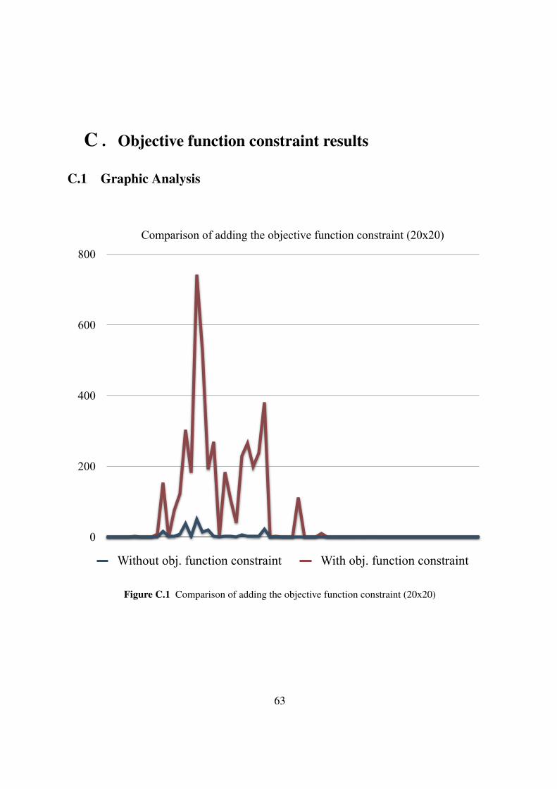
C . Objective function constraint results

C.1 Graphic Analysis

0

200

400

600

800

Comparison of adding the objective function constraint (20x20)

Without obj. function constraint With obj. function constraint

Figure C.1 Comparison of adding the objective function constraint (20x20)

63

64

0

125

250

375

500

Comparison of adding the objective function constraint (40x60)

Without obj. function constraint With obj. function constraint

Figure C.2 Comparison of adding the objective function constraint (40x60)

C.2 Full Results

Table C.1: Objective Function Constraint Full Results (in seconds)

Title Dens. Logic time ILP Total Time ILP Objective TotalTime

TEST_40x60x5_101 10% 0,004008 (timeout) (timeout)TEST_40x60x5_102 10% 0,007015 (timeout) (timeout)TEST_40x60x5_103 10% 0,004186 (timeout) (timeout)TEST_40x60x5_104 10% 0,004052 (timeout) (timeout)

Continued on Next Page. . .

65

Table C.1 – Continued

Title Dens. Logic time ILP Total Time ILP Objective TotalTime

TEST_40x60x5_105 10% 0,006514 (timeout) (timeout)TEST_40x60x5_106 10% 0,007298 (timeout) (timeout)TEST_40x60x5_107 10% 0,004339 (timeout) (timeout)TEST_40x60x5_108 10% 0,004539 (timeout) (timeout)TEST_40x60x5_109 10% 0,006905 (timeout) (timeout)TEST_40x60x5_110 10% 0,007397 (timeout) (timeout)TEST_40x60x5_201 20% 0,010571 (timeout) (timeout)TEST_40x60x5_202 20% 0,009854 (timeout) (timeout)TEST_40x60x5_203 20% 0,009511 (timeout) (timeout)TEST_40x60x5_204 20% 0,01521 (timeout) (timeout)TEST_40x60x5_205 20% 0,01081 (timeout) (timeout)TEST_40x60x5_206 20% 0,0103 (timeout) (timeout)TEST_40x60x5_207 20% 0,011707 (timeout) (timeout)TEST_40x60x5_208 20% 0,009916 (timeout) (timeout)TEST_40x60x5_209 20% 0,010247 (timeout) (timeout)TEST_40x60x5_210 20% 0,010717 (timeout) (timeout)TEST_40x60x5_301 30% 0,015882 (timeout) (timeout)TEST_40x60x5_302 30% 0,016525 (timeout) (timeout)TEST_40x60x5_303 30% 0,011587 (timeout) (timeout)TEST_40x60x5_304 30% 0,012335 (timeout) (timeout)TEST_40x60x5_305 30% 0,012559 (timeout) (timeout)TEST_40x60x5_306 30% 0,012374 (timeout) (timeout)TEST_40x60x5_307 30% 0,011737 (timeout) (timeout)TEST_40x60x5_308 30% 0,017578 (timeout) (timeout)TEST_40x60x5_309 30% 0,01167 (timeout) (timeout)TEST_40x60x5_310 30% 0,017201 (timeout) (timeout)TEST_40x60x5_401 40% 0,014588 (timeout) (timeout)TEST_40x60x5_402 40% 0,016404 (timeout) (timeout)TEST_40x60x5_403 40% 0,020021 (timeout) (timeout)TEST_40x60x5_404 40% 0,021128 (timeout) (timeout)TEST_40x60x5_405 40% 0,017274 (timeout) (timeout)TEST_40x60x5_406 40% 0,01655 (timeout) (timeout)TEST_40x60x5_407 40% 0,015545 (timeout) (timeout)TEST_40x60x5_408 40% 0,016417 (timeout) (timeout)TEST_40x60x5_409 40% 0,020481 (timeout) (timeout)TEST_40x60x5_410 40% 0,018087 (timeout) (timeout)TEST_40x60x5_501 50% 0,007589 4,687589 93,587589TEST_40x60x5_502 50% 0,009948 38,719948 396,849948TEST_40x60x5_503 50% 0,008944 6,218944 145,838944TEST_40x60x5_504 50% 0,008441 7,738441 415,878441

Continued on Next Page. . .

66

Table C.1 – Continued

Title Dens. Logic time ILP Total Time ILP Objective TotalTime

TEST_40x60x5_505 50% 0,008051 4,608051 81,808051TEST_40x60x5_506 50% 0,010827 707,860827 (timeout)TEST_40x60x5_507 50% 0,010493 214,130493 292,440493TEST_40x60x5_508 50% 0,009045 62,669045 6,919045TEST_40x60x5_509 50% 0,007846 41,897846 92,327846TEST_40x60x5_510 50% 0,007829 10,227829 17,597829TEST_40x60x5_601 60% 0,004593 2,634593 2,624593TEST_40x60x5_602 60% 0,004935 2,844935 2,804935TEST_40x60x5_603 60% 0,004945 2,704945 2,664945TEST_40x60x5_604 60% 0,005493 2,705493 2,645493TEST_40x60x5_605 60% 0,005037 2,725037 2,685037TEST_40x60x5_606 60% 0,004871 2,724871 2,674871TEST_40x60x5_607 60% 0,004406 2,664406 2,644406TEST_40x60x5_608 60% 0,004729 2,814729 2,764729TEST_40x60x5_609 60% 0,00489 2,90489 2,80489TEST_40x60x5_610 60% 0,004983 4,124983 3,004983TEST_40x60x5_701 70% 0,00369 2,26369 2,25369TEST_40x60x5_702 70% 0,003786 2,303786 2,273786TEST_40x60x5_703 70% 0,003813 2,193813 2,173813TEST_40x60x5_704 70% 0,004106 2,304106 2,274106TEST_40x60x5_705 70% 0,003826 2,243826 2,223826TEST_40x60x5_706 70% 0,003975 2,273975 2,243975TEST_40x60x5_707 70% 0,003604 2,113604 2,083604TEST_40x60x5_708 70% 0,00359 2,21359 2,18359TEST_40x60x5_709 70% 0,003752 2,223752 2,143752TEST_40x60x5_710 70% 0,003718 2,133718 2,093718TEST_40x60x5_801 80% 0,002892 1,802892 1,702892TEST_40x60x5_802 80% 0,00315 1,86315 1,77315TEST_40x60x5_803 80% 0,003001 1,873001 1,783001TEST_40x60x5_804 80% 0,002906 1,802906 1,702906TEST_40x60x5_805 80% 0,002639 0,002639 0TEST_40x60x5_806 80% 0,003013 1,883013 1,793013TEST_40x60x5_807 80% 0,003058 1,873058 1,743058TEST_40x60x5_808 80% 0,002934 1,772934 1,692934TEST_40x60x5_809 80% 0,00299 1,88299 1,78299TEST_40x60x5_810 80% 0,003019 1,883019 1,783019TEST_40x60x5_901 90% 0,002046 0,002046 0TEST_40x60x5_902 90% 0,001976 1,171976 1,081976TEST_40x60x5_903 90% 0,002093 1,212093 1,122093TEST_40x60x5_904 90% 0,002019 1,212019 1,122019

Continued on Next Page. . .

67

Table C.1 – Continued

Title Dens. Logic time ILP Total Time ILP Objective TotalTime

TEST_40x60x5_905 90% 0,002246 1,262246 1,152246TEST_40x60x5_906 90% 0,002194 1,152194 1,072194TEST_40x60x5_907 90% 0,001974 0,001974 0TEST_40x60x5_908 90% 0,00185 0,00185 0TEST_40x60x5_909 90% 0,00225 1,23225 1,14225TEST_40x60x5_910 90% 0,001817 1,221817 1,131817TEST_20x20x5_101 10% 0,000412 0,230412 0,170412TEST_20x20x5_102 10% 0,000514 0,250514 0,150514TEST_20x20x5_103 10% 0,000401 0,200401 0,160401TEST_20x20x5_104 10% 0,000381 0,320381 0,180381TEST_20x20x5_105 10% 0,000381 0,240381 0,240381TEST_20x20x5_106 10% 0,000458 0,430458 1,160458TEST_20x20x5_107 10% 0,000407 0,260407 0,180407TEST_20x20x5_108 10% 0,000592 0,480592 0,270592TEST_20x20x5_109 10% 0,000443 0,350443 0,220443TEST_20x20x5_110 10% 0,00043 0,47043 8,36043TEST_20x20x5_201 20% 0,001093 15,121093 153,171093TEST_20x20x5_202 20% 0,000755 1,130755 0,350755TEST_20x20x5_203 20% 0,000656 1,370656 75,190656TEST_20x20x5_204 20% 0,000852 7,410852 122,340852TEST_20x20x5_205 20% 0,001033 37,101033 302,441033TEST_20x20x5_206 20% 0,000938 1,940938 182,410938TEST_20x20x5_207 20% 0,000654 50,740654 743,040654TEST_20x20x5_208 20% 0,00094 13,93094 526,07094TEST_20x20x5_209 20% 0,000839 19,730839 190,530839TEST_20x20x5_210 20% 0,000634 1,500634 269,610634TEST_20x20x5_301 30% 0,001106 0,831106 0,931106TEST_20x20x5_302 30% 0,001051 2,451051 182,721051TEST_20x20x5_303 30% 0,001098 1,501098 106,611098TEST_20x20x5_304 30% 0,000966 0,700966 39,420966TEST_20x20x5_305 30% 0,001128 6,351128 230,371128TEST_20x20x5_306 30% 0,000761 2,380761 264,460761TEST_20x20x5_307 30% 0,00083 30,42083 (timeout)TEST_20x20x5_308 30% 0,001057 1,361057 198,901057TEST_20x20x5_309 30% 0,000952 1,050952 238,120952TEST_20x20x5_310 30% 0,000759 22,870759 381,070759TEST_20x20x5_401 40% 0,000969 0,390969 0,320969TEST_20x20x5_402 40% 0,000972 0,470972 1,320972TEST_20x20x5_403 40% 0,000805 0,420805 0,380805TEST_20x20x5_404 40% 0,001082 0,331082 0,301082

Continued on Next Page. . .

68

Table C.1 – Continued

Title Dens. Logic time ILP Total Time ILP Objective TotalTime

TEST_20x20x5_405 40% 0,000881 0,430881 0,370881TEST_20x20x5_406 40% 0,001177 0,901177 111,051177TEST_20x20x5_407 40% 0,000804 0,380804 0,320804TEST_20x20x5_408 40% 0,000934 0,310934 0,290934TEST_20x20x5_409 40% 0,000943 0,350943 0,330943TEST_20x20x5_410 40% 0,001006 0,561006 10,051006TEST_20x20x5_501 50% 0,000784 0,390784 0,350784TEST_20x20x5_502 50% 0,000725 0,250725 0,250725TEST_20x20x5_503 50% 0,00075 0,24075 0,24075TEST_20x20x5_504 50% 0,000775 0,240775 0,270775TEST_20x20x5_505 50% 0,000717 0,220717 0,210717TEST_20x20x5_506 50% 0,000785 0,330785 0,310785TEST_20x20x5_507 50% 0,00073 0,23073 0,25073TEST_20x20x5_508 50% 0,000821 0,260821 0,270821TEST_20x20x5_509 50% 0,000754 0,370754 0,360754TEST_20x20x5_510 50% 0,000759 0,280759 0,270759TEST_20x20x5_601 60% 0,000686 0,200686 0,210686TEST_20x20x5_602 60% 0,000605 0,230605 0,250605TEST_20x20x5_603 60% 0,000652 0,210652 0,200652TEST_20x20x5_604 60% 0,00074 0,21074 0,21074TEST_20x20x5_605 60% 0,000771 0,240771 0,230771TEST_20x20x5_606 60% 0,000636 0,200636 0,210636TEST_20x20x5_607 60% 0,000736 0,210736 0,210736TEST_20x20x5_608 60% 0,000646 0,000646 0TEST_20x20x5_609 60% 0,00073 0,22073 0,23073TEST_20x20x5_610 60% 0,000677 0,230677 0,230677TEST_20x20x5_701 70% 0,000572 0,190572 0,190572TEST_20x20x5_702 70% 0,000529 0,180529 0,180529TEST_20x20x5_703 70% 0,000496 0,000496 0TEST_20x20x5_704 70% 0,000504 0,000504 0TEST_20x20x5_705 70% 0,000559 0,190559 0,190559TEST_20x20x5_706 70% 0,000538 0,200538 0,200538TEST_20x20x5_707 70% 0,000502 0,000502 0TEST_20x20x5_708 70% 0,00058 0,19058 0,19058TEST_20x20x5_709 70% 0,000493 0,000493 0TEST_20x20x5_710 70% 0,000493 0,000493 0TEST_20x20x5_801 80% 0,000435 0,000435 0TEST_20x20x5_802 80% 0,00045 0,16045 0,15045TEST_20x20x5_803 80% 0,000411 0,000411 0TEST_20x20x5_804 80% 0,000434 0,000434 0

Continued on Next Page. . .

69

Table C.1 – Continued

Title Dens. Logic time ILP Total Time ILP Objective TotalTime

TEST_20x20x5_805 80% 0,000397 0,000397 0TEST_20x20x5_806 80% 0,000418 0,000418 0TEST_20x20x5_807 80% 0,000428 0,150428 0,150428TEST_20x20x5_808 80% 0,000476 0,160476 0,160476TEST_20x20x5_809 80% 0,000442 0,000442 0TEST_20x20x5_810 80% 0,000422 0,140422 0,150422TEST_20x20x5_901 90% 0,000285 0,000285 0TEST_20x20x5_902 90% 0,000297 0,000297 0TEST_20x20x5_903 90% 0,000314 0,000314 0TEST_20x20x5_904 90% 0,000295 0,000295 0TEST_20x20x5_905 90% 0,000316 0,000316 0TEST_20x20x5_906 90% 0,000303 0,000303 0TEST_20x20x5_907 90% 0,000313 0,000313 0TEST_20x20x5_908 90% 0,000339 0,000339 0TEST_20x20x5_909 90% 0,000358 0,000358 0TEST_20x20x5_910 90% 0,000305 0,000305 0

Legend:

Title: Title of the nonogramDens.: Global density of the nonogramLogic time: Time spent logically solving the nonogramILP Total Time: Total time spent solving the nonogram using the hybrid approach, includ-

ing the time spent logically solving itILP Objective Total Time: Total time spent solving the nonogram using the hybrid ap-

proach with the objective function constraint, including the time spent logically solving it

D . Nonogram File Formats

D.1 Bosch based file format

title: TEST_20x20x5_101number_of_rows: 20number_of_columns: 20number_of_colors: 5

row_1:number_of_clusters: 3size(s): 1 1 1color(s): 1 1 1

row_2:number_of_clusters: 1size(s): 1color(s): 1

row_3:number_of_clusters: 3size(s): 1 3 1color(s): 1 1 2

row_4:number_of_clusters: 1size(s): 1color(s): 1

row_5:number_of_clusters: 3size(s): 1 1 1color(s): 2 2 2

row_6:number_of_clusters: 0size(s):color(s):

row_7:71

72

number_of_clusters: 0size(s):color(s):

row_8:number_of_clusters: 1size(s): 1color(s): 2

row_9:number_of_clusters: 2size(s): 1 1color(s): 3 3

row_10:number_of_clusters: 0size(s):color(s):

row_11:number_of_clusters: 5size(s): 1 1 1 1 1color(s): 3 3 4 3 3

row_12:number_of_clusters: 3size(s): 1 1 1color(s): 3 3 3

row_13:number_of_clusters: 2size(s): 1 1color(s): 4 4

row_14:number_of_clusters: 2size(s): 1 1color(s): 4 4

row_15:number_of_clusters: 1

73

size(s): 1color(s): 4

row_16:number_of_clusters: 3size(s): 1 2 1color(s): 4 4 1

row_17:number_of_clusters: 2size(s): 1 1color(s): 5 1

row_18:number_of_clusters: 2size(s): 1 1color(s): 5 5

row_19:number_of_clusters: 2size(s): 1 1color(s): 5 5

row_20:number_of_clusters: 1size(s): 1color(s): 5

column_1:number_of_clusters: 0size(s):color(s):

column_2:number_of_clusters: 1size(s): 1color(s): 1

column_3:number_of_clusters: 0size(s):

74

color(s):

column_4:number_of_clusters: 1size(s): 1color(s): 4

column_5:number_of_clusters: 3size(s): 2 1 1color(s): 3 5 5

column_6:number_of_clusters: 2size(s): 1 1color(s): 2 1

column_7:number_of_clusters: 2size(s): 1 1color(s): 1 3

column_8:number_of_clusters: 1size(s): 2color(s): 3

column_9:number_of_clusters: 4size(s): 1 1 1 1color(s): 1 4 4 5

column_10:number_of_clusters: 2size(s): 1 1color(s): 1 3

column_11:number_of_clusters: 4size(s): 1 1 1 1color(s): 1 2 4 4

75

column_12:number_of_clusters: 2size(s): 2 1color(s): 1 3

column_13:number_of_clusters: 1size(s): 1color(s): 1

column_14:number_of_clusters: 1size(s): 1color(s): 4

column_15:number_of_clusters: 5size(s): 1 1 1 2 1color(s): 1 3 3 4 4

column_16:number_of_clusters: 2size(s): 1 1color(s): 2 5

column_17:number_of_clusters: 1size(s): 1color(s): 5

column_18:number_of_clusters: 1size(s): 1color(s): 2

column_19:number_of_clusters: 3size(s): 1 1 1color(s): 2 1 5

76

column_20:number_of_clusters: 0size(s):color(s):

D.2 Olšák file format

Title: TEST_20x20x5_101#da:a 1b:b 2c:c 3d:d 4e:e 5

: rows1a 1a 1a1a1a 3a 1b1a1b 1b 1b

1b1c 1c

1c 1c 1d 1c 1c1c 1c 1c1d 1d1d 1d1d1d 2d 1a1e 1a1e 1e1e 1e1e: columns

1a

1d

77

2c 1e 1e1b 1a1a 1c2c1a 1d 1d 1e1a 1c1a 1b 1d 1d2a 1c1a1d1a 1c 1c 2d 1d1b 1e1e1b1b 1a 1e

: end

D.3 Hett based file format

specimen_nonogram(’TEST_20x20x5_101’,[[[1,1],[1,1],[1,1]][[1,1]][[1,1],[3,1],[1,2]][[1,1]][[1,2],[1,2],[1,2]][][][[1,2]][[1,3],[1,3]][][[1,3],[1,3],[1,4],[1,3],[1,3]][[1,3],[1,3],[1,3]][[1,4],[1,4]][[1,4],[1,4]][[1,4]][[1,4],[2,4],[1,1]][[1,5],[1,1]][[1,5],[1,5]][[1,5],[1,5]]

78

[[1,5]]],[[][[1,1]][][[1,4]][[2,3],[1,5],[1,5]][[1,2],[1,1]][[1,1],[1,3]][[2,3]][[1,1],[1,4],[1,4],[1,5]][[1,1],[1,3]][[1,1],[1,2],[1,4],[1,4]][[2,1],[1,3]][[1,1]][[1,4]][[1,1],[1,3],[1,3],[2,4],[1,4]][[1,2],[1,5]][[1,5]][[1,2]][[1,2],[1,1],[1,5]][]]).--------------------------------

Bibliography

[1] The eclipse constraint programming system. http://www.eclipse-clp.org/.

[2] Griddlers net. http://www.griddlers.net/.

[3] Ilog cplex. http://www.ilog.com/products/cplex/.

[4] Scip: Solving constraint integer programs. http://scip.zib.de/.

[5] Egon Balas and Robert Jeroslow. Canonical cuts on the unit hypercube. SIAM Journal onApplied Mathematics, 23(1):61–69, 1972.

[6] Colin Barker. LPA Win-Prolog Goodies. http://pagesperso-orange.fr/colin.barker/lpa/lpa.htm.

[7] Robert A. Bosch. Painting by numbers. Optima, (65):16–17, May 2001. Also availablehere http://www.oberlin.edu/math/faculty/bosch/pbn.ps.

[8] Ali Corbin. Ali corbin’s home page. http://www.blindchicken.com/~ali/.

[9] Brian Grainger. Pencil puzzles and sudoku. http://www.icpug.org.uk/national/features/050424fe.htm.

[10] Werner Hett. Hett nonogram solver in prolog. https://prof.ti.bfh.ch/hew1/informatik3/prolog/p-99/.

[11] Javier Larrosa and Enric Morancho. Solving ’still life’ with soft constraints andbucket elimination. In Francesca Rossi, editor, Principles and Practice of ConstraintProgramming-CP 2003: 9th International Conference, CP 2003, Kinsale, Ireland,September 29-October 3, 2003 : Proceedings, pages 466–479, Kinsale, Ireland, 2003.Springer.

[12] Luís Mingote and Francisco Azevedo. Colored nonograms: an integer linear program-ming approach. In Lopes et al., editor, Progress in Artificial Intelligence, 14th PortugueseConference on Artificial Intelligence, EPIA 2009, Aveiro, Portugal, 2009. Springer.

[13] Mirek Olšák and Petr Olšák. Griddlers solver, nonogram solver. http://www.olsak.net/grid.html#English.

[14] Joachim Schimpf. ECLiPSe Code Samples. http://eclipse.crosscoreop.com/examples/.

[15] Steven Simpson. Nonogram programs. http://www.comp.lancs.ac.uk/~ss/software/nonowimp/.

79

80

[16] Steven Simpson. Nonogram solver. http://www.comp.lancs.ac.uk/~ss/nonogram/.

[17] Steven Simpson. Nonogram solver - solvers on the web. http://www.comp.lancs.ac.uk/~ss/nonogram/list-solvers.

[18] Jung-Fa Tsai, Ming-Hua Lin, and Yi-Chung Hu. Finding multiple solutions to generalinteger linear programs. European Journal of Operational Research, 184(2):802–809,2008.

[19] Nobuhisa Ueda and Tadaaki Nagao. Np-completeness results for nonogram via parsimo-nious reductions. Technical Report TR96-0008, Tokyo Institute of Technology (Titech),Department of Computer Science, http://www.cs.titech.ac.jp/~tr/reports/1996/TR96-0008.ps.gz, May 1996.

[20] Wouter Wiggers. A comparison of a genetic algorithm and a depth first search algorithmapplied to japanese nonograms. Paper, Faculty of EECMS, University of Twente, 2004.

[21] Wikipedia. Nonogram. http://en.wikipedia.org/wiki/Nonogram.

[22] Jan Wolter. The ’pbnsolve’ paint-by-number puzzle solver. http://webpbn.com/pbnsolve.html.

[23] Jan Wolter. Survey of paint-by-number puzzle solvers. http://webpbn.com/survey/.