UNIVERSIDADE NOVA DE LISBOA Faculdade de Ciências e Tecnologia ...run.unl.pt/bitstream/10362/5118/1/Calvário_2010.pdf · UNIVERSIDADE NOVA DE LISBOA Faculdade de Ciências e Tecnologia

UNIVERSIDADE NOVA DE LISBOA

Faculdade de Ciências e Tecnologia

Departamento de Engenharia Mecânica e Industrial/Secção de

Tecnologia Industrial

Modelling a Cable Structure for a New Wind Energy Production

Device

Por

Miguel Pita Soares da Fonseca Calvário

2ºCiclo

Lisboa

2010

Orientador: Prof. Jorge Joaquim Pamies Teixeira

Co-orientador: Eng.º Tiago Pardal

Dissertação apresentada na Faculdade de Ciências e

Tecnologia da Universidade Nova de Lisboa para obtenção do

grau de Mestre em Engenharia Mecânica Especialização em

Concepção e Produção

Acknowledgements

i

Acknowledgements

Writing this thesis was only possible due the collaboration of several persons, to which I want

to express my thanks, especially:

To my supervisor, Prof. Jorge Joaquim Pamies Teixeira, I thank the opportunity to

develop this thesis and for the different meetings, suggestions and guidance (have in

mind his long experience) during the supervising process;

To OMNIDEA, for the challenge of participating on this innovative project. I’m

particulate grateful to my co-supervisor, Eng.º Tiago Pardal, for availability of

commercial information, to Eng.º Pedro Silva for his opinions and special support on

the computational domain and to Eng.º Nuno Fernandes for his suggestions to the

structure of thesis.

To Prof. João Burguete Cardoso for the support given on the modulation and analysis

of the cable structure;

To teachers and partners of Faculdade de Ciências e Tecnologia of Universidade Nova

de Lisboa and Escola Superior de Tecnologia of Instituto Politécnico de Setúbal that

contributed to my engineering formation.

Abstract

iii

Abstract

The following thesis subject is based on the identification and dimensioning of the main

mechanical components of the ground station of Boreas prototype, as well as a three-

dimensional finite element analysis of structural cable that connects the ground station to the

module's air system. The module powered by a lift force pulls a cable that drives a mechanical

system which in turn drives a generator during the productive phase of the energy cycle. In

the other phase, the system inverts the turn and energy is consumed. The production of energy

should be greater than the energy consume.

The dimensioning of main mechanical components of ground station includes: flywheel,

cable, capstan drum and winder drum.

Structural analysis of the cable is performed with an algorithm based on a three-dimensional

finite element analysis, which allows the control of cable tension on the end of capstan,

prevent the rupture of cable, avoid high forces on bearings and the shock between the rope

and the ground. The results of programme developed with the algorithm, are compared with

the results obtained by an analytical approach and with commercial software of finite

elements.

This thesis contributes to the realization of mechanical components included in the prototype.

Keywords: mechanical system, cable, modulation of finite elements

Resumo

iv

Resumo

A presente tese tem como objectivos a identificação e dimensionamento dos principais

componentes mecânicos da estação terrestre do protótipo Boreas, bem como uma análise

tridimensional de elementos finitos do cabo estrutural que une a estação terrestre ao módulo

aéreo do protótipo. O módulo aéreo movido por uma força de sustentação aerodinâmica puxa

um cabo que acciona um sistema mecânico que por sua vez conduz um gerador durante a fase

produtiva do ciclo energético. Na outra fase do ciclo, o sistema inverte o sentido do

movimento, consumindo energia. A produção energética deverá superar o consumo

energético.

O dimensionamento dos principais componentes mecânicos da estação terrestre inclui:

volante, cabo, tambores do cabrestante e enrolador.

A análise estrutural do cabo é desenvolvida através de um algoritmo baseado numa análise de

tridimensional de elementos finitos, permitindo o controlo da tensão de cabo no apoio situado

no cabrestante, previne a ruptura do cabo, evita forças elevadas nos rolamentos e o choque

entre o cabo e o chão. Os resultados do programa desenvolvido com o algoritmo são

comparados com os resultados obtidos por um método analítico e por um software comercial

de elementos finitos.

Esta tese contribui para a materialização dos componentes mecânicos incluídos no protótipo.

Palavras-chave: sistema mecânico, cabo, modulação por elementos finitos

Nomenclature

v

Nomenclature

Constants of integration

Diameter of electric cable

External diameter of the ring

External diameter of gas tube

Diameter of flange

Inner diameter of the ring

Internal diameter of gas tube

Young modules of UHMPE

Young modules of steel

Force on winder drum

Force of unwinding

Force on capstan drum

Drag force

Maximum force of operation

Minimum force of operation

Weight of their own half of the distributed force

Total length of cable

Length of winder

Results from programmes or analytical solution

Results from software

Axial force on the vertex of catenary

Unitary Volume of electric cable

Unitary Volume of gas tube

Total weight of cable

Weight of catenary cable for unit of length

Weight of the electric cable for unit of length

Weight of elements

Weight of gas tube for unit of length

Weight of structural cable for unit of length

Vector of total displacements (iteration i)

Nomenclature

vi

Vector of total displacements (iteration i+1)

Internal forces

External forces vector

Internal forces vector

Initial length (m)

Length of cable

Length of catenary

Length of parabola

Length of cable for a certain loop

Projection of element in the three orthogonal axes

Number of elements

Pressure on capstan drum

Pressure on winder drum

Inner radius of capstan drum

Outer radius of capstan drum

Radius of shaft

Radius of cable

External Radius of capstan drum

Inner Radius of capstan drum

Radius of the pack (winder drum+ loops of cable)

Radius of winder drum

External radius of winder drum

Internal radius of winder drum

Variable radius between an

Thickness of flywheel

Thickness of capstan drum

Thickness of winder drum

Nodal coordinates

Radial strain

Tangential strain

Density of polyamide

Density of cooper

Nomenclature

vii

Density of steel

Principal stresses

Stress of service

Ultimate stress on cable

Ultimate stress on capstan drum

Maximum allowable stress on cable

Maximum allowable stress on capstan drum

Maximum stress on cable

Radial stress

Tangential stress

Tangential stress due external pressure on winder drum

Tangential stress due the rotation of winder drum

Angular speed of motor

Incremental displacement vector

FEM Finite element method

UHMPE Ultra high molecular polyethylene

Diameter of capstan drum

Young modules

Energy lost

Energy stored

Energy stored effectively

Energy

Approximation error

Inertia moment of flywheel

Tangent stiffness matrix

Minimum breaking force

Power

Relation of the load side and hold side

Maximum relative error

Minimum relative error

Relative error

Relation between and

Safety factor for cable

Nomenclature

viii

Safety factor for capstan drum

Axial force on a point

Constant parameter of the curve

Diameter of structural cable

Acceleration of gravity

Number of turns in section

Sub-matrix

Deformed length

Inner radius of cylinder

Tensile stress

Time

Displacement of the cylindrical surface of radius r

Speed

Abscissa of a point

Ordinate of a point

Area of cross section

Friction coefficient

Lagrange-Green strain

Poisson ratio

Uniform stress on the element

Angular speed of capstan

Cylinder external radius of

Cylinder inner radius of

General index

ix

General index

Acknowledgements ..................................................................................................................... i

Abstract ...................................................................................................................................... iii

Resumo ...................................................................................................................................... iv

Nomenclature.............................................................................................................................. v

General index ............................................................................................................................. ix

Figures index ........................................................................................................................... xiii

Tables index .............................................................................................................................. xv

1. Introduction ......................................................................................................................... 1

2. Thesis structure ................................................................................................................... 3

3. State of art of wind technologies ......................................................................................... 5

3.1. The wind resource ........................................................................................................ 5

3.2. Wind technologies ....................................................................................................... 7

3.2.1. Reference to wind turbines ................................................................................... 7

3.2.2. Mention to MARS project .................................................................................. 10

4. Structure of Boreas prototype ........................................................................................... 11

4.1. Specifications produced by OMNIDEA .................................................................... 12

4.2. Description of mechanical components of the ground station ................................... 13

5. Dimensioning the main mechanical components of ground station of Boreas prototype . 15

5.1. Energy considerations ................................................................................................ 15

5.2. Energy behaviour of system ...................................................................................... 16

5.3. Dimensioning the flywheel ........................................................................................ 18

5.4. Dimensioning the cable ............................................................................................. 20

5.4.1. Initial considerations .......................................................................................... 20

5.4.2. Determination of structural cable diameter ........................................................ 22

5.4.3. Real cross section of cable.................................................................................. 24

General index

x

5.5. Dimensioning the capstan drum ................................................................................ 26

5.5.1. Non-rotating thick cylinder ................................................................................ 26

5.5.2. Rotating thick cylinder ....................................................................................... 29

5.5.3. Pressure on the capstan drum ............................................................................. 29

5.5.4. Results ................................................................................................................ 31

5.6. Dimensioning the winder drum ................................................................................. 33

6. Modelling the cable structure ........................................................................................... 37

6.1. Analytical equations to study cable structures .......................................................... 37

6.2. FEM ........................................................................................................................... 38

6.2.1. Methodology of resolution using the FEM ........................................................ 42

6.2.2. FEM on cable structures .................................................................................... 43

6.2.3. Newton-Raphson method ................................................................................... 50

6.3. Programme evaluation ............................................................................................... 52

6.3.1. Analytical solution ............................................................................................. 53

6.3.2. Programme’s solution ........................................................................................ 55

6.3.3. Software solution ............................................................................................... 60

6.3.4. Analysis of results .............................................................................................. 62

6.4. Structural analysis of cable........................................................................................ 66

6.4.1. Initial geometry .................................................................................................. 67

6.4.2. Section properties ............................................................................................... 67

6.4.3. Loads .................................................................................................................. 68

7. Conclusions and future work ............................................................................................ 73

References ................................................................................................................................ 75

Annex 1 – List of MATLAB mfile .......................................................................................... 77

Annex 2 – Input file of programme’s A version ...................................................................... 83

Annex 3 – “Input” file of programme’s B version ................................................................... 85

Annex 4 –ANSYS log file ....................................................................................................... 87

General index

xi

Annex 5- Input file of programme for the structural analysis of cable example ...................... 91

Figures index

xiii

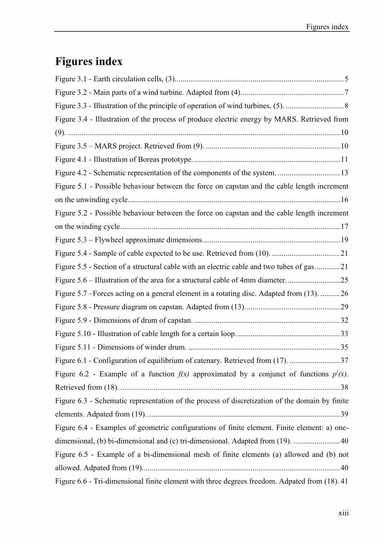
Figures index

Figure 3.1 - Earth circulation cells, (3). ...................................................................................... 5

Figure 3.2 - Main parts of a wind turbine. Adapted from (4). .................................................... 7

Figure 3.3 - Illustration of the principle of operation of wind turbines, (5). .............................. 8

Figure 3.4 - Illustration of the process of produce electric energy by MARS. Retrieved from

(9). ............................................................................................................................................ 10

Figure 3.5 – MARS project. Retrieved from (9). ..................................................................... 10

Figure 4.1 - Illustration of Boreas prototype. ........................................................................... 11

Figure 4.2 - Schematic representation of the components of the system. ................................ 13

Figure 5.1 - Possible behaviour between the force on capstan and the cable length increment

on the unwinding cycle. ............................................................................................................ 16

Figure 5.2 - Possible behaviour between the force on capstan and the cable length increment

on the winding cycle. ................................................................................................................ 17

Figure 5.3 – Flywheel approximate dimensions. ...................................................................... 19

Figure 5.4 - Sample of cable expected to be use. Retrieved from (10). ................................... 21

Figure 5.5 - Section of a structural cable with an electric cable and two tubes of gas. ............ 21

Figure 5.6 – Illustration of the area for a structural cable of 4mm diameter. ........................... 25

Figure 5.7 –Forces acting on a general element in a rotating disc. Adapted from (13). .......... 26

Figure 5.8 - Pressure diagram on capstan. Adapted from (13). ................................................ 29

Figure 5.9 - Dimensions of drum of capstan. ........................................................................... 32

Figure 5.10 - Illustration of cable length for a certain loop. ..................................................... 33

Figure 5.11 - Dimensions of winder drum. .............................................................................. 35

Figure 6.1 - Configuration of equilibrium of catenary. Retrieved from (17). .......................... 37

Figure 6.2 - Example of a function f(x) approximated by a conjunct of functions pi(x).

Retrieved from (18). ................................................................................................................. 38

Figure 6.3 - Schematic representation of the process of discretization of the domain by finite

elements. Adpated from (19). ................................................................................................... 39

Figure 6.4 - Examples of geometric configurations of finite element. Finite element: a) one-

dimensional, (b) bi-dimensional and (c) tri-dimensional. Adapted from (19). ........................ 40

Figure 6.5 - Example of a bi-dimensional mesh of finite elements (a) allowed and (b) not

allowed. Adpated from (19)...................................................................................................... 40

Figure 6.6 - Tri-dimensional finite element with three degrees freedom. Adpated from (18). 41

Figures index

xiv

Figure 6.7 - Example of a beam element with a rotation degree of freedom. Adapted from

(18). .......................................................................................................................................... 41

Figure 6.8 – Schematic representation of methodology of finite element analysis. Adapted

from (19). ................................................................................................................................. 43

Figure 6.9 - Finite basic element. Adapted from (17). ............................................................. 44

Figure 6.10 - Discretization of cable (n+1 nodes and n elements). Retrieved from (17). ....... 44

Figure 6.11 - Cartesian coordinates of internal forces. Retrieved from (17). .......................... 46

Figure 6.12 - Equilibrium of forces on node i. Adapted from (17).......................................... 46

Figure 6.13 - Newton-Raphson method Adapted from (17). ................................................... 50

Figure 6.14 – Illustration of a cable with two fixed ends. ....................................................... 52

Figure 6.15 - Illustration of the coordinates of point T. ........................................................... 53

Figure 6.16 - Illustration of the initial configuration proposed and position of the reference of

coordinates of cable on programme. ........................................................................................ 55

Figure 6.17 - Illustration of the deformed geometry for programme’s A version. .................. 57

Figure 6.18 - Illustration of the deformed geometry for programme’s B version. .................. 58

Figure 6.19 - Illustration of the deformed geometry according to ANSYS software. ............. 60

Figure 6.20 – Schematically diagram of external forces applied on structure. ........................ 68

Figure 6.21 - Illustration of the deformed geometry. ............................................................... 70

Tables index

xv

Tables index

Table 5.1 – Energy specifications for a typical situation. ........................................................ 15

Table 5.2 - Value of energy to be stored. ................................................................................. 17

Table 5.3 - Considerations to the calculus of inertia moment. ................................................. 18

Table 5.4 - Value of maximum allowed stress on the cable. Adapted from (10). .................... 20

Table 5.5 – Variables to determinate for a value of 3 (mm). ............................................ 22

Table 5.6 - Variables to determinate for value of 4 (mm). ................................................ 22

Table 5.7 - Variables to determinate . .............................................................................. 23

Table 5.8 - Variables to determinate . ............................................................................. 24

Table 5.9 - Total value of weight of gas tubes. ........................................................................ 24

Table 5.10 - Weight of cable and of the different components. ............................................... 24

Table 5.11 - Variables to determine the external pressure and length of capstan. ................... 30

Table 5.12 - Maximum and minimum values of the radial and tangential stress on the drum of

capstan considering a non-rotating cylinder. ............................................................................ 31

Table 5.13 - Maximum and minimum values of the tangential stress on the drum of capstan

considering a rotating cylinder. ................................................................................................ 31

Table 5.14 - Variables to determine the maximum allowable stress on capstan. ..................... 31

Table 5.15 - Maximum allowable stress, tangential stress and thickness of capstan. .............. 32

Table 5.16 - Geometric characteristics of winder..................................................................... 34

Table 6.1 - Characteristics of cable. ......................................................................................... 52

Table 6.2 - Coordinates of deformed geometry. ....................................................................... 54

Table 6.3 - Values of tension, stress and length obtained by the model of catenary................ 54

Table 6.4 - Coordinates of nodes of the initial geometry. ........................................................ 56

Table 6.5 - Displacements on nodes and global coordinates of deformed nodes for

programme’s A version. ........................................................................................................... 57

Table 6.6 -Internal forces on the elements for programme’s A version. .................................. 58

Table 6.7 - Displacements on nodes for programme’s B version. ........................................... 59

Table 6.8 - Internal forces on the elements for programme’s B version. ................................. 59

Table 6.9 - Displacements on nodes for software. ................................................................... 60

Table 6.10 - Internal forces on the elements for software. ....................................................... 61

Table 6.11 – Comparison of deformed geometry between the analytical equation and

software. ................................................................................................................................... 62

Tables index

xvi

Table 6.12 - Relative error for displacements between programme’s A version and software.

.................................................................................................................................................. 63

Table 6.13 - Relative error for displacements between programme’s B version and software.

.................................................................................................................................................. 64

Table 6.14 . Relative error for internal forces between analytical equation and software. ...... 64

Table 6.15 - Relative error for internal forces between programme’s A version and software.

.................................................................................................................................................. 65

Table 6.16 - Relative error for internal forces between programme’s B version and software.

.................................................................................................................................................. 65

Table 6.17 - Section properties of cable. ................................................................................. 67

Table 6.18 - Coordinates of nodes incremental length of cable and forces on nodes. ............. 69

Table 6.19 - Description of elements and corresponding nodes. ............................................. 69

Table 6.20 - Value of displacements on nodes. ....................................................................... 70

Table 6.21 - Value of forces on elements. ............................................................................... 71

1. Introduction

1

1. Introduction

The tendencies for future solutions of wind energy production, in opposition to actual wind

systems (for example wind turbines), are constituted by aero structures, lighter than air. In this

way the system, which is described, is an aero structure that work in cycles of high altitudes

(more than 500 meters) being connected to a capstan on the ground. This system is coupled to

an electric generator, producing energy during a part of cycle. The system is currently

patented, [1].

The importance of working with the wind of high altitudes is reflected on the electric power.

The value of wind speed increases with the increasing of altitude and the electrical power

generated by wind turbines in the process of energy transformation shows a cubic dependence

on wind speed, so small variations in wind speed represent large variations on value of

electric power, [2]. The wind speed at 450 meters can be four or five times higher than in the

ground, [2], and its flow is more stable than the earth surface reducing the problem of

seasonality.

The objectives of this thesis are the identification and dimensioning of the main mechanical

components of the ground station (flywheel, cable, capstan drum and winder drum) of Boreas

prototype as well as a three-dimensional finite element analysis of structural cable that

connects the ground station to the module's air system. Under the scientific point of view, the

modelling of cable structure is studied to allow the determination of stresses and cable

trajectory. The importance of knowing which is the tension on the rope for the different nodes

and the angle between cable and ends is to prevent the rupture of cable, avoid high forces on

bearings and avoid the shock between the rope and the ground (which creates too friction on

cable). The displacements (due the elasticity of cable and value of loads) are an important

issue taking into account the limited area of work.

On the future work other components as the support structure of the drum, the structure of

anchoring to the ground, the control system, etc, should be studied in order to complete the

design of prototype.

2. Thesis structure

3

2. Thesis structure

The thesis is structured in 7 chapters. Chapter 1 consists on an introduction to the general

environment of wind energies where considerations about the importance of wind of high

altitudes are mentioned. The chapter continues with a short description of the mechanical

system and the future work. Chapter 3 presents a state of art of wind technologies where the

characteristics of wind resource and the technologies that take part of it are in discussion.

Chapter 4 refers to a description of the characteristics of the “Boreas” prototype, where the

elements of the mechanical device are mentioned.

The chapter 5 is related to the energy considerations and with the dimensioning of major

mechanical components of ground station (flywheel, cable, capstan drum, winder,

respectively). In this way data is provide for the design of prototype.

On chapter 6, the methodology and proposed modelling of cable structure is presented

considering two possible approaches based on analytical equations or the finite element

method. Later in the chapter an algorithm characterizing the behaviour of cable submitted to

forces is proposed. This algorithm will be important for the control programme of the device.

On chapter 7 the thesis conclusion is presented and the future work to be done is proposed.

Lastly, the thesis has 5 annexes being the first one related to the list of MATLAB file, the

Annex 2 and 3 represent the input files of programme’s A and programme’s version B, the

Annex 4 specifies the ANSYS file and on Annex 5 is shown the input file of the structural

analysis of cable example.

3. State of art of wind technologies

5


This topic, after an introduction to the thematic of wind resource, describes the major

technologies that take part from the wind resource in order to produce energy; in particular

electric energy.

3.1. The wind resource

The wind can be characterized as air in motion with a certain intensity and direction. It is the

result from displacement of air masses, as a result of pressure differences between two distinct

regions. The pressure differences are associated with solar radiation and heating processes of

air masses: the high pressure air descends and departs heating to converge and where the low

rises, [2]. The heating areas of land and sea are different from the poles to the tropics, causing

the displacement of heat flows between these zones, being the wind one of carriers of heat

flows. The wind would always flow perpendicular to the isobars if the influence of rotation of

the earth does not induced small deviations in the flow of wind through the action of Coriolis

forces, [2].

Figure 3.1 - Earth circulation cells, [3].

Other important issue are the breezes, which refers to the flow localized wind with lower

intensity. The breezes result from the unequal heating or cooling of land surfaces, on a certain

location. The most common breezes are, [2]:


6

Land breeze - Wind that blows during the night of earth surface into the sea, in that, on

the earth surface the temperature decreases more quickly in the night, compared with

sea water, creating a difference of pressure; high pressures on the earth surface and

low pressures on the sea;

Sea breeze - Wind that blows during the day, from the sea to earth surface and as

result of the earth surface warm more quickly than sea water during the day, a

difference of pressure is created; high pressures on the sea and low pressures on the

earth;

Valley breeze - Winds that blows in the morning from the valley to the mountains

peaks and, as a result of the mountains peaks warm faster than the valleys, a difference

of pressure is creating; high pressures on the valley and low pressures on the mountain

peaks.

The increase of altitude increase the wind speed, due the roughness, orography but also

because the air is denser on the earth surface, decreasing the density with height, [2]. The

wind speed don’t increases infinitely with the increase of height from the ground, it can be to

450 meters four or five times higher than in the ground but at higher levels the relation

decreases, [2].

The knowledge of the wind behaviour is determinate to introduce the technology on a certain

place in order to adjust parameters, as the height or orientation of structure.


7

3.2. Wind technologies

The wind technologies are one type of the renewable energies and are characterized specially

by the wind turbines.

3.2.1. Reference to wind turbines

The wind energy can be described as the transformation of energy provided by wind on a

useful energy, generally electricity. The most known way to produce wind energy is the use of

wind turbines, which drive an electric generator.

The main components that constituted the wind turbines are:

Blade – Component that is orientated to wind direction in order to rotate;

Hub – Joint of blades with the shaft, which will transmit horse power;

Nacelle – Component that includes: the anemometer, bearings, rotor, gearbox,

generator, coupling, disk brake yaw system, etc.

Tower – Element that brings height to structure;

Foundation – Element that holds the tower and others components to ground.

Figure 3.2 - Main parts of a wind turbine. Adapted from [4].


8

The principle that allows the transformation of wind energy in electric energy is described as

a result of using the aerodynamic principles; in particular two primary aerodynamic forces:

lift force, in the direction perpendicular to wind flow, and drag force in direction parallel to

wind flow. The turbine blades use an airfoil design, in which one surface is nearly rounded

and the other is relatively flat. When the wind flows into the rounded surface, the air is forced

to rise, increasing velocity. The faster moving air tends to rise in the atmosphere due to a

decrease in pressure just above of the curved surface. On the upwind side of the blade, the

wind is moving slower,creating an area of higher pressure that pushes on the blade, trying to

slow it down. This difference in pressure implies that the low-pressure area sucks the blade

towards the wind flow, creating the lift force that is perpendicular to drag force, [5].

Figure 3.3 - Illustration of the principle of operation of wind turbines, [5].

The aerodynamic principles are not the only parameters on the design of wind turbines. For

example the size of blade is quite important because the longer be the turbine blades are,

greater is the diameter of the rotor and more energy can be produced. As a rule, doubling the

rotor diameter produces a four times more energy. However it must to be taken into account

that the increase of inertia on the system requires more power to spin the generator and

therefore a trade should be obtained between these aspects.

The tower height is also an important parameter in production capacity, heaving in mind that

higher elevations allow higher wind speed because, at the ground friction and heights of


9

objects interrupt the wind of flow, reducing the wind speed, [5]. In this way higher turbines

can capture more energy.

In order to calculate the power of the wind turbine is important to know the wind velocity at

the place of implementation and nominal capacity of wind turbine (dimensions, rotor diameter

and other). The major part of turbines reach their maximum power at speeds of wind near 15

(m/s), and if be considerate stable winds the rotor diameter determinates the quantity of

energy to produce. At the time that rotor diameter increases, the height of the tower increase

as well, which allows to access to faster winds, [5].

It is important to note that at 15 (m/s) the generality of turbines reach his nominal capacity

and at 20 (m/s) the system is shut down, [5], because at that wind speeds the structure can

collapse specially due the large vibrations.

At a global scale, the installed capacity by the end of 2009 reached 158.505 (MW) and 38.343

(MW) were added, [6]. The average capacity of wind turbines installed globally in 2007 was

1492 (kW), [7] , and the largest turbines on the market have now 6 (MW) in capacity, [8].


10

3.2.2. Mention to MARS project

At the moment, a new dispositive called MARS (Magenn Power Air Rotor System) is being

developed and it consists on a rotor device, lighter than air that rotates about a horizontal axis

due the wind and his rotation is converted into electrical energy. The electrical energy is

transported down to a transformer at a ground station; being transported to the electricity

power grid. The air rotor is sustained by helium and the rotor lights to the more adequate

altitudes taking in account the wind speed, which also causes the Magnus effect creating

additional lift which keeps the device stabilized and positioned, [9].

Figure 3.4 - Illustration of the process of produce electric energy by MARS. Retrieved

from [9].

Figure 3.5 – MARS project. Retrieved from [9].

4. Structure of prototype Boreas”

11

4. Structure of Boreas prototype

The tendencies for future solutions of wind energy production, in opposition to actual wind

systems, are constituted by aero structures, lighter than air. In this way the system, which is

described, is an aero structure that work in cycles of high altitudes (more than 500 meters)

being connected to a capstan on the ground. This system is coupled to an electric generator,

producing energy during a part of cycle. The cycle consists of two phases, one productive;

where the aero module is lifted pulling the cable that drives a mechanical system that in turn

drives a generator. On a second phase, the module comes down by the rewinding the using

generator that in this cycle is wired to work as an electric engine. Special clutch arrangement

will be needed in order to change in the mechanical actions.

Figure 4.1 - Illustration of Boreas prototype.

4. Structure of prototype Boreas

12

4.1. Specifications produced by OMNIDEA

The initial specifications produced by OMNIDEA established the following items:

Length of cable: 750 (m);

Typical height range of operation: 150-450 (m);

Angle typical operation of cable (surface-winch-module air): 40 to 60 degrees;

Maximum power on unwinding: 120 (kW) (typical situation of speed of unwinding 4

(m/s), tension (30000 (N));

Maximum tension and speed on unwinding: 50000 (N) and 6 m/s (not simultaneous);

Maximum power on winding: 80 (kW) (typical situation of speed of unwinding 8

(m/s), tension (10000 (N));

Maximum tension and speed on winding: 20000 (N) and 12 (m/s), (not simultaneous);

Lifecycle of equipment: 20 years (more than 1000 000 cycles);

System must be transportable in a TIR container standard;

The cable section should be circular and allow the accommodation of gas tubes and

electric cables.

4. Structure of prototype Boreas

13

4.2. Description of mechanical components of the ground station

The mechanical components of the ground station contain the main items represented on

Figure 4.2.

flywheelmotor /

generator

clutch /

brake systemmechanical

system inversioncapstan

Figure 4.2 - Schematic representation of the components of the system.

On the unwinding cycle the system is coupled, producing energy. The winding begins with

the uncoupling the shaft of capstan and the shaft of generator, by the clutch, and then the

brake system is actuated to immobilize the capstan. Completed this operation, the mechanical

system inversion reverses the rotation of capstan and during the period of time that the

capstan needs to reach the rated speed, the flywheel will provide the needed energy. In this

way a high pulse of electricity consumption by the system is avoided. Achieved the nominal

speed the motor/generator switches to the motor mode (mode power consumption).

Finishing the winding cycle, the clutch is again actuated in order to uncouple the shaft of

capstan and shaft of motor; the brake is actuated again in order to immobilize the capstan. The

mechanical system inversion reverses the rotation of capstan and its shaft is again coupled

with shaft of motor and for then, the motor switches to generator mode.

The system needs also a winding drum to store the cable. All these components must be

anchored to the ground and must have the capability of rotation to orient adequately the cable

as the wind direction varies.

5. Dimensioning the main components of ground station of prototype Boreas

15

5. Dimensioning the main mechanical components of

ground station of Boreas prototype

On this chapter is proposed the methodology of dimensioning the equipment of system that

the development of system should have. Some assumptions are done because is difficult to

know exactly some project parameters due to impossibility of test the system. The following

considerations are related to the main mechanical components of ground station of prototype.

5.1. Energy considerations

The energy generated during unwinding can be written by (5.1).

(5.1)

Assuming constant speed, the time is given by (5.2).

(5.2)

Take into account the specifications of the device for a typical situation, the specifications of

energy are presented on Table 5.1.

Table 5.1 – Energy specifications for a typical situation.

Cycle (kW) (m) (m/s) (s) (kJ)

Winding 80 500 8 62.5 5000

Unwinding 120 500 4 125 15000


16

5.2. Energy behaviour of system

For both cycles, the energy has two regimes: transient and stationary taking into account

parameters as the lift force or the inertia of system.

In the end of winding cycle, the system already rewound the totality of the cable in operation,

so the system will reverse the movement and the nominal force on capstan to unwind should

be 30 000 (N), in order to produce 15000 (kJ) of useful energy. The transition between

coupling shaft capstan to the motor will produce an overshoot of force, beyond the required

one as shown on the Figure 5.1. The maximum value depends on the characteristics of the

mechanical system.

30 000

50000

0

Fcapstan (N)

Δl (m)

Stationary regimeTransient regime

Figure 5.1 - Possible behaviour between the force on capstan and the cable length

increment on the unwinding cycle.

At the end of unwinding cycle ends, the motor will be uncoupled from capstan, which is

locked and rotation of capstan is reversed. The flywheel will provide power to the motor

during a certain period of time, so that it reaches the nominal winding speed (until the

nominal force of rewinding reaches nearly 10 000 (N)). Again a transient regime will occur as

shown on Figure 5.2. In the same manner, the overshoot will depend from the characteristics

of system.


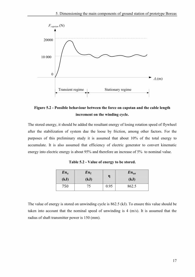
17

10 000

20000

0

Fcapstan (N)

Δl (m)

Stationary regimeTransient regime

Figure 5.2 - Possible behaviour between the force on capstan and the cable length

increment on the winding cycle.

The stored energy, it should be added the resultant energy of losing rotation speed of flywheel

after the stabilization of system due the loose by friction, among other factors. For the

purposes of this preliminary study it is assumed that about 10% of the total energy to

accumulate. It is also assumed that efficiency of electric generator to convert kinematic

energy into electric energy is about 95% and therefore an increase of 5% to nominal value.

Table 5.2 - Value of energy to be stored.

(kJ)

(kJ) η

(kJ)

75 0.95 862.5

The value of energy is stored on unwinding cycle is 862.5 (kJ). To ensure this value should be

taken into account that the nominal speed of unwinding is 4 (m/s). It is assumed that the

radius of shaft transmitter power is 150 (mm).


18

5.3. Dimensioning the flywheel

The value of kinetic energy of flywheel that should be accumulated is given by (5.3):

(5.3)

So the inertia moment of flywheel is obtained by (5.4).

(5.4)

The angular speed is related to the angular speed of engine which is assumed 1500

(rpm).

Table 5.3 - Considerations to the calculus of inertia moment.

(m)

(rad/s)

(kJ)

(kg m2)

0.325 (*) 157.080 862.5 69.911

The inertia moment for hollow cylinder is described by (5.5).

(5.5)

In order to achieve the value of inertia moment, geometry of flywheel is proposed of Figure

5.3.


19

Figure 5.3 – Flywheel approximate dimensions.


20

5.4. Dimensioning the cable

This topic is related to specification the section of cable take into account that the cross

section is not available.

5.4.1. Initial considerations

The determination of the normal stress that the cable can have during the cycles of operation

is brought by (5.6).

(5.6)

The determination of ultimate stress is given by (5.7).

(5.7)

The maximum allowable stress is obtained by (5.8).

(5.8)

According to the specifications, the maximum tension of service on cable is 50000 (N). The

manufacturer of cable, EURONEEMA, specifies the MBF for a certain value of external

surrounding diameter. The chosen value for is 3. The characteristics of cable and the

variables to the determine the maximum allowable stress are presented on Table 5.4.

Table 5.4 - Value of maximum allowed stress on the cable. Adapted from [10].

(m)

[10-3

]

(m2)

[10-4

]

Weight

(kg/100 m)

(kN)

(kN)

(MPa)

(MPa)

6 0.283 2.2 35 50 1768.659 412.687

8 0.503 4 62 50 994.629 411.113

10 0.785 6 97 50 636.618 411.680

12 1.131 9.3 137 50 442.087 403.772

14 1.539 10.7 184 50 324.886 398.527

16 2.011 15 244 50 248.633 404.442

18 2.545 19.6 303 50 196.464 396.857

20 3.142 23.1 374 50 159.134 396.775


21

The areas expressed in Table 5.4 refer to filled sections, although the section of cable

expected to be implemented, is a combination of elliptical coils that have voids between them.

It would be necessary to analyse several samples from different sections of cable in order to

determinate a medium value of area. The material of the cable is UHMPE with commercial

name of EURONEEMA.

Figure 5.4 - Sample of cable expected to be use. Retrieved from [10].

The value of area is related to a diameter of 14 (mm) because in this section the service stress

is the nearest of the respective maximum allowable stress.

The project requires that the cable has a structural hollows section to allow the passage of

electric cable and gas tubes. The section houses an electrical cable with 8 (mm) of diameter,

housed in the inner section and two gas pipes with a thickness of 4 (mm) being the inner

diameter, , of 12.2 (mm). Considering the structural cable, the section of cable has

geometry of a ring represented on Figure 5.5.

Figure 5.5 - Section of a structural cable with an electric cable and two tubes of gas.

The external diameter of the ring, ,, takes into account and the diameter of structural

cable , being expressed by (5.9).

(5.9)


22

In this way the area is obtained by (5.10).

(5.10)

5.4.2. Determination of structural cable diameter

In order to determinate , a 3 (mm) structural cable is tested, being the results on Table 5.5.

Table 5.5 – Variables to determinate for a value of 3 (mm).

(m)

[10-3

]

(m)

[10-3

]

(m)

[10-3

]

(m2)

[10-4

]

12.2 3 18.2 1.433

For inner diameter, with 12.2 (mm), and a structural cable with 3 (mm) of diameter displayed

on a ring, the area is less than the reference area value, 1.539x10-4

(m2). In this way a ring with

the referred inner diameter, with a structural cable of 4 (mm), will be evaluated, being the

results on Table 5.6

Table 5.6 - Variables to determinate for value of 4 (mm).

(m)

[10-3

]

(m)

[10-3

]

(m)

[10-3

]

(m2)

[10-4

]

12.2 4 20.2 2.036

For a ring with 4 (mm) of thickness, and an inner diameter of 20.2 (mm) the value of area is

higher than the reference value, so the condition is validated.

5.4.2.1. Determination of the weight of the different cables

In this topic the weight of structural cable, electrical cable and gas tubes are proposed.

5.4.2.1.1. Weight of structural cable unit of length

From the Table 5.4, the weight of structural cable can be estimated by the following relation:


23

(kg/m)

(kg/m)

So the value of is:

(kg/m)

The transformation of weight of structural cable in kg/m to N/m is given by (5.11).

(N/m) (5.11)

5.4.2.1.2. Weight of electric cable for unit of length

The weight of the electric cable for unit of length is given by (5.12).

(5.12)

The value of is given by (5.13).

(5.13)

Take into account the considerations; it obtains a value of shown on Table 5.7.

Table 5.7 - Variables to determinate .

(m)

[10-3

] (kg /m

3) (m s

-2)

(m2)

[10-5

] (kg /m) (N/m)

8 8910, [11] 9.807 5.027 0.448 4.393

5.4.2.1.3. Weight of gas tube for unit of length

The weight of gas tube for unit of length is obtained by (5.14).


24

(5.14)


(5.15)

Take into account the considerations; it obtains a value of shown on Table 5.8.

Table 5.8 - Variables to determinate .

(m)

[10-3

]

(m)

[10-3

] (kg /m

3)

(m2)

[10-6

]

(kg/m)

[10-3

]

(N/m)

[10-2

]

4 2.7 1400, [12] 6.841 9.577 9.393

This weight must be multiply by 2, because there are two tubes. So:

Table 5.9 - Total value of weight of gas tubes.

(kg/m) [10-2

] (N/m)

1.915 0.188

5.4.2.1.4. Total weight of cable

The total weight of cable is given by (5.16) being the results on Table 5.10.

(5.16)

Table 5.10 - Weight of cable and of the different components.

(kg /m) (kg /m) [10-2

] (kg/m) (kg /m) (N/m)

0.141 1.915 0.448 0.608 5.963

5.4.3. Real cross section of cable

The cable is a combination of sections that on a first assumption are considered as circulars,

existing interstices (voids) between them so it is necessary verify which is the effective area,

considering an outer diameter of 20.2 (mm).


25

Figure 5.6 – Illustration of the area for a structural cable of 4mm diameter.

A structural cable with circumferences of 4 (mm), has a value of area, , of 1.557x10-4

(m2),

which is bigger than the reference value , 1.539x10-4

(m2). So the area of reference is checked.

Considering that the space occupied by ellipses in the ring is greater than circumferences, it is

estimated that the area is higher than the actual resistance value of a structural cable with

circumferences of 4 (mm). So it will be used the value of area of 1.539x10-4

(m2), with the

weight of cable of 5.963 (N/m), knowing that these values are not overestimated on a large

scale.


26

5.5. Dimensioning the capstan drum

On this topic the dimensions of capstan drum is proposed and verified to the loads.

5.5.1. Non-rotating thick cylinder

Assuming the model of thick cylinder submitted to pressure, the study is based on a static

approach. The procedure developed elsewhere [13] is used. Further details can be obtained

there.

dθ

a1

ab

b1

drdr

σdσ

rr

σ

σ r

σ

r

dr

a

a1

b

b1

ri

r0

Figure 5.7 –Forces acting on a general element in a rotating disc. Adapted from [13].

A constant thick cylinder thickness, where acting internal and external pressures distributed

on a uniform way. The deformation is symmetric relatively to the cylinder axis and his value

don´t vary at the length of cylinder.

An element of the cylinder ab-a1b1, Figure 5.7, with unitary thickness that for symmetric

reason will not occur shear stress on the focus of the selected element. The is the tangential

stress normal to faces aa1 e bb1 and be the radial stress normal to ab face. This stress is

function of r and vary .

The sum of the projections of forces based on the bisector of angle , not considering the

self weight, gives the equilibrium equation (5.17).


27

(5.17)

If the higher order infinitesimals were neglected, obtains the equation (5.18).

(5.18)

The deformation on the cylinder is symmetric and a radial displacement of all points of the

wall is the same. The deformation is constant on the circumferential direction, but varies

radially. If is the displacement of the cylindrical surface of radius r, for the surface of radius

, the displacement is given by (5.19)

(5.19)

The unit radial strain is brought by (5.20).

(5.20)

The unit tangential strain is given by (5.21).

(5.21)

In this way the stress equations can be written by the equation (5.22).

(5.22)

If these values be substituted on the equilibrium equation, the result is the following

differential equation (5.23).

(5.23)


28

The general solution is given by (5.24).

(5.24)

So it obtains the equations (5.25) and (5.26).

(5.25)

(5.26)

The constants and are determinate by boundary conditions, which refer to the value of

external pressure and internal pressure. The value of constants can be written by (5.27) and

(5.28).

(5.27)

(5.28)

These expressions when inserted on (5.25) (5.26), allows the achievement of (5.29) and

(5.30).

(5.29)

(5.30)

The value of + is constant and the deformation is the same for all the elements, so planar

sections remains planar after the deformation. For the particular case, is 0 which means that

the internal pressure is 0, so it finally obtains the equations (5.31) and (5.32).

(5.31)


29

(5.32)

The value of is maximum for , is maximum for , and these

stresses are always compressive stresses.

5.5.2. Rotating thick cylinder

A thin thick-walled cylinder with constant thickness, with an outer radius , an inner radius

in rotation with a constant angular speed ω, with a density ρ and a Possion´s ratio µ, has a

tangential stress, [14]:

(5.33)

5.5.3. Pressure on the capstan drum

The pressure applied by the cable into the drum of capstan can be determinate if we consider

one half of drum, being the equilibrium given by (5.34).

Fcapstan

pcapstan

Fcapstan

Figure 5.8 - Pressure diagram on capstan. Adapted from [13].

(5.34)

Solving equation (5.34), it is obtained the expression (5.35).

(5.35)


30

The length of capstan depends from number of turns that the capstan drum can have. So the

number of turns take into account the relation of , the load side, and tension that goes

to winder drum, , hold side, being brought it by (5.36).

(5.36)

Establishing a relation , between and the value of is given by (5.37)

(5.37)

The length of capstan drum depends from number of turns that the capstan drum can have,

and the external diameter of cable, being given by (5.38).

(5.38)

Bearing in mind that the quotient between the diameter of capstan and diameter of cable

should, at least, be equal or greater than 30, according to manufacturer of cable

(LANKHORST EURONETE ROPES, S.A.), so a diameter of capstan of 650 (mm) is chosen.

Table 5.11 - Variables to determine the external pressure and length of capstan.

(N)

(m)

(rad)

Nº of

spires

(m)

(m)

(m)

(m)

50000 0.1 10 69.078 11 0.0041 0.0202 0.65 0.222

Sizing the capstan with one more spire, with 4 (mm) of spacing between the spires and a

margin of 20 (mm) flanges on each side until the flanges result on a length of capstan of 331.7

(mm).


31

5.5.4. Results

Considering a non-rotating cylinder the results are expressed on Table 5.12.

Table 5.12 - Maximum and minimum values of the radial and tangential stress on the

drum of capstan considering a non-rotating cylinder.

(MPa)

0 -172.415

-24.485 -147.930

Considering rotation on the cylinder the tangential stress is expressed on Table 5.13.

Table 5.13 - Maximum and minimum values of the tangential stress on the drum of

capstan considering a rotating cylinder.

(Mpa)

-172.296

-172.319

So the maximum value of tangential stress of compression of 172.415 (MPa). The maximum

allowable stress of capstan is obtained by (5.39).

(5.39)

The material, ultimate stress the safety of factor chosen, admit the maximum allowable stress

on capstan, expressed on Table 5.14.

Table 5.14 - Variables to determine the maximum allowable stress on capstan.

Designation (MPa) (MPa)

Steel (S355), [11] 355, [11] 2 177.5

The values of and , allow a thickness on capstan drum presented on Table 5.15.


32

Table 5.15 - Maximum allowable stress, tangential stress and thickness of capstan.

(MPa) (Mpa) (mm)

177.5 -172.415 50

The dimensions of capstan are illustrated on Figure 5.9.

Figure 5.9 - Dimensions of drum of capstan.


33

5.6. Dimensioning the winder drum

In order to determinate the radius of drum, the total length of cable is an important parameter,

shown on obtained by (5.40), and shown on Figure 5.10.

Figure 5.10 - Illustration of cable length for a certain loop.

(5.40)

The length of cable for a certain loop is given by (5.41).

(5.41)


(5.42)

The total length of cable is given take into account the length of cable on a certain loop and is given by

(5.43):

(5.43)

The diameter of flanges is given by (5.44).

(5.44)


34

Taking into account that the total of length of cable is 750 m, the parameters where adjusted

in order to reach a value of length of cable near the reference value.

Table 5.16 - Geometric characteristics of winder.

(m) (m) [10

-3] (m) N (m)

0.4 20.2 0.75 7 38 1.083

The model of shell (curve plate of thin wall), by membrane theory, can be used. It is assumed:

Stresses are constant on the thickness of shell;

The quotient between the thickness/radius of curvature is less than 1/20;

There is a stress plain ( two principal stress);

Low deformations, the bigger deformation is less than half of the thickness of shape;

Secondary stresses are not evaluated.

For a cylindrical shell, the tangential stress, also called hoop stress, is given by (5.45), [11].

(5.45)

Due the rotation of the winder, another tangential stress is given by (5.46), [15].

(5.46)

The total tangential stress is given by (5.47).

(5.47)

Using the Tresca criterion, this leads to (5.48).

(5.48)

Considering plane stress, =0, therefore (5.49).


35

(5.49)

The value of for different spires of winding can be approximate to (5.50) , [16].

(5.50)

The value of , is given by (5.51).

(5.51)

The tension to apply to cable on the winder should be the minimum possible, ideally null, in

order to reduce the friction. So the expressions presented represent a methodology for the

determination of thickness of winder but have in mind that the tension on cable when goes to

winder is low, the thickness of winder is determinate by the manufacturing process. Knowing

the lathe process will be used is proposed a value of 30 (mm) to the sheet, that will be curved

and then welded.

Figure 5.11 - Dimensions of winder drum.

6. Modelling the cable structure

37


As referred earlier, one of the main objectives of this thesis is the cable modelling, in order to

determine the stresses involved and the estimation of trajectory of the cable. In this way, two

approaches are exposed in order to give answers to the control of device.

6.1. Analytical equations to study cable structures

Usually the cable structures are analyzed with simplified analytical equations, such as the

catenary equation, in which the cable supported on two rigid ends requested by a load

uniformly distributed along its axis, such as the self-weight of the cable, [17].

Figure 6.1 - Configuration of equilibrium of catenary. Retrieved from [17].

The equations that described the behaviour of catenary are, [17]:

(6.1)

(6.2)

(6.3)

(6.4)


38

6.2. FEM

The finite element method is a numerical method (approximate method), where the domain of

problem is decomposed into several sub domains. In each of these sub domains, the equations

that regulate the phenomenon are approximated by a variational method. The approximation

of a solution into several sub domains allows an easier representation of a complicated

function by a composition of simple polynomials functions where the error can be as small as

desired, simply increasing the number of sub domains, [18].

Figure 6.2 - Example of a function f(x) approximated by a conjunct of functions pi(x).

Retrieved from [18].

In Figure 6.2 the function, f(x) depicted as solid line, is approximated by the polynomials

pi(x), represented at red, (p

1(x), p

2(x)… p

8(x)). The polynomials are defined on sub domains,

di, and at the time that the number of sub domains increase, lesser is the error on the

approximation.

The FEM requires the utilization of the variational principles (principle of virtual work, the

principle of stationary potential energy or the principle of Hamilton, etc) because the problem

must be formulated as a defined integral in the whole domain, in other words, the sets of

equations that describe the physical phenomena establish relationships between the variables

and the parameters of the problem on the neighbourhood of each point, so in order to pass this

description of the physical phenomenon to the integral description, it is necessary to use the

variational principles, [18].


39

The FEM is a stratified methodology: it can be used to solve one-dimensional problems, but

generally is applied to problems where the solution is an area or a generic tri-dimensional

volume. In any of these cases the first step is divide on finite number of segments, areas or

volumes smaller, called finite elements. This process is the discretization, [19]. On the Figure

6.3 is shown the schematic representation of the process of discretization of the domain by

finite elements.

y

xO

Boundary

O

y

x

Domain

Element

Node

Figure 6.3 - Schematic representation of the process of discretization of the domain by

finite elements. Adpated from [19].

The finite elements can have different geometric shapes, being one-dimensional, bi-

dimensional or tri-dimensional.

To solve one-dimensional problems (or consisting of one-dimensional elements) the finite

elements have the shape of segments. On bi-dimensional problems the elements are frequently

quadrilaterals or triangles and for tri-dimensional problems the elements can be hexahedral,

tetrahedral, pentahedral, etc.


40

(a) (b) (c)

Figure 6.4 - Examples of geometric configurations of finite element. Finite element: a)

one-dimensional, (b) bi-dimensional and (c) tri-dimensional. Adapted from [19].

Considering a linear elastic analysis of general problems in engineering, usually in FEM the

first step is to determine the field of displacements of a finite number of points in system.

These points are the nodes of the mesh of finite element, which are on vertex of elements, as

it shown on and Figure 6.5. Is important note that depending of the type of formulation in

finite element analysis, the nodes can be on the edges, on their faces or inside them. The

nodes that belong to the boundary of adjacent elements must be common to all elements that

exist there. For this reason is not possible the discretization of a solid medium in elements that

do not coincide on their own nodes.

(a) (b)

Figure 6.5 - Example of a bi-dimensional mesh of finite elements (a) allowed and (b) not

allowed. Adpated from [19].

In this way the numerical analysis done with the finite element method, on a first step,

calculates the node displacements for a certain load on the domain under analysis. So the

displacement of each point of the finite element can be determined by the displacements of


41

the nodes on that element, which is, according to the nodal displacements. In this way the

calculation of the displacements of a finite number of elements (the nodes of the mesh) allows

the determination of an infinite number of points of a continuous domain. In other words, the

displacement of any point can be defined according the displacements of the nodes of the

element that the point belong, [19].

For example on a bi-dimensional, the displacement of each node can be decomposed in two

perpendicular components, one parallel to a reference axis Ox and other parallel to a reference

axis Oy. These components of displacement are called degrees of freedom. On a bi-

dimensional case each node has two degrees of freedom, concerning the axis Ox and Oy.

Analogously for a tri-dimensional finite element each node has three degrees freedom, have in

mind the relationship between that point with the three orthogonal spatial directions.

x2

x1

x3

uIIuI

vIIvI

wIIwI

Figure 6.6 - Tri-dimensional finite element with three degrees freedom. Adpated from

[18].

If a problem is discretized with n of nodes, so the total number of degrees of freedom is the

product of n by the number of degrees of freedom for node. With the increasing of the total

number of degrees of freedom of the system, more time is required for the calculus. Besides

the displacement, the variables can be also nodal degrees of freedom of rotation.

x2

x1

x3

vIIvI

θIIθI

Figure 6.7 - Example of a beam element with a rotation degree of freedom. Adapted

from [18].


42

When the displacements are calculated, the numeric simulation software calculates the

respective deformation and its stresses. Then the information is shown to the programmer in

order to be analysed.

6.2.1. Methodology of resolution using the FEM

On a generally approach the tasks that a programmer do when is doing a simulation

programme by the FEM are insert in three different stages:

Pre-processing (i);

Analysis (ii);

Post-processing (iii).

6.2.1.1. Pre-processing

The pre-processing phase represents the construction of a geometric model of a system,

including the loads and conditions of the problem. In commercial software this phase includes

graphic tools that allow the user, to build easily the model of system to analyze. On this phase

the user defines the parameters, namely the type of finite element, the mesh, mechanical

properties, loads (forces, moments, pressure, etc), boundary conditions (constraints), so the

global quality of the analysis is directly affected by the accuracy of the inputs.

This information is the input data to the system. In order to reduce the calculation time and

the information generated, the user defines the set of results needed. When completed, the

files of input data are submitted to the analysis phase.

6.2.1.2. Analysis

The analysis is the phase of process of numeric simulation by the FEM that the calculus is

done. The phase begins with the verification of the information input on the file data, created

by the user, and if no errors be detected the numeric simulation is done, being created output

files with all information that user required.

6.2.1.3. Post-processing

The post-processor is the module that outputs the information of the result output files,

through graphic tools or schedules, and the information displayed should be user-friendly. For


43

example the graphic tools can be coloured distributions of isovalues or isocolours. The post-

processor can be included with the others items of the programme, in order to do the use of

the programme easily and uniform. The different phases of a typical analysis of finite

elements, on the point of view of user, can be summarized and systemized on Figure 6.8.

Definition of concept

Analysis

Model

Geometry definition, nodes, elements,

boundary layers, materials, loads.

Definition of parameters and analysis

control.

Interpretation

Representaion of results

Results evaluation:

Displacements, forces, stresses,

deformations, etc.

Results representation:

Isovalues, contours, history of

variables in time, animations, etc.

Pre-processing

EndPost-processing

Figure 6.8 – Schematic representation of methodology of finite element analysis.

Adapted from [19].

6.2.2. FEM on cable structures

In order to study the cable, a finite element the procedure developed elsewhere [17] is used.

Further details can be obtained there.


44

6.2.2.1. Discretization of the finite element mesh

The element to use in this study is of cable type. It has two nodes on ends and three

orthogonal independent displacements, where are a continuous series of elements connected

by labelled link, submitted to nodal forces and large displacements.

Figure 6.9 - Finite basic element. Adapted from [17].

Figure 6.10 - Discretization of cable (n+1 nodes and n elements). Retrieved from [17].

The initial length, before the deformation, defines the initial configuration, which is calculated

with the nodal coordinates. The initial length is given by (6.5).

(6.5)

The vector of nodal displacements associated to the element, is defined

by the three independent displacements of the two end nodes defining the element. This

vector and the initial configuration will define the deformed configuration and the deformed

length (6.6).

(6.6)


45

The direction of the displacement of each element is calculated by (6.7), (6.8) and (6.9).

(6.7)

(6.8)

(6.9)

6.2.2.2. Equilibrium conditions

The equilibrium on the three orthogonal directions, in which node of structure, is defined by

equation (6.10).

(6.10)

The incremental vector is the unknown variable to be determinate. Due to the large

displacements, the geometry is not constant, the stiffness coefficients and the internal forces

depend on the geometry and therefore on the deformed configuration, [17].

The methodology of resolution of problem consists on an iterative strategy, and when the

convergence is achieved, the deformed configuration and internal forces can be calculated.

6.2.2.2.1. Internal and external forces

Due to equilibrium the resultants of external forces and internal forces must be equal. The

components of internal forces on a node are a function of the axial load acting on element,

which depends from the deformed configuration (Figure 6.11), so the initial configuration and

a vector of displacements are needed to obtain the internal forces. The six components of

internal forces in the element are: , where, (6.11) :

(6.11)


46

Figure 6.11 - Cartesian coordinates of internal forces. Retrieved from [17].

The global axial force F on the element is obtained by (6.12):

(6.12)

The stress is a function of the field of displacements and is calculated by the constitutive law

of material. The elastic linear (Hook’s) law is given by (6.13).

(6.13)

Taking into consideration that large displacements are considered, the Lagrangian formulation

was used. The stiffness coefficients and internal forces where calculated with the definition of

Lagrange-Green strain, (6.14).

(6.14)

The external forces allocated on the nodes of extremity are defined by the vector:

.

Figure 6.12 - Equilibrium of forces on node i. Adapted from [17].


47

The equilibrium conditions should be satisfied in each direction and for all nodes. The

conditions of equilibrium for the three directions are given by (6.15), (6.16) and (6.17).

(6.15)

(6.16)

(6.17)

6.2.2.2.2. Stiffness matrix

The stiffness matrix coefficients of the cable element are not linear because the geometry is

not constant; so the tangent matrix stiffness characterizes

the stiffness. The global tangent stiffness at cable, , has a dimension

and is obtained by the assembly of the tangent stiffness of each element, , (a matrix with

dimension ), obtained by (6.18).

(6.18)

- Sub-matrix is given by

(6.19)

Knowing that:

(6.20)

The matrix elements can be obtained by (6.21) and (6.22).

(6.21)


48

(6.22)

where

Therefore the six coefficients of tangent stiffness matrix are obtained by equation (6.23) to

(6.28):

(6.23)

(6.24)

(6.25)

(6.26)

(6.27)

(6.28)

where:

(6.29)

(6.30)

(6.31)


49

(6.32)

(6.33)


50

6.2.3. Newton-Raphson method

In order to resolve (6.10), an iterative process based on the Newton-Raphson method is

implemented. The calculation begins with the input the initial values of stiffness and internal

forces; so initial values of the vector of displacements must be given; in this way an initial

geometry and deformed geometry must be defined.

Assuming the equilibrium and linear behaviour, the equation (6.34) is valid in all nodes.

(6.34)

This equation is resolved and the vector increment of displacement is calculated and a new

vector of total displacements is obtained by: (6.35).

(6.35)

di di+1 di+2

fi

fi+1

fi+2

d

f

Δi Δi+1

Δf i

Δf i

+1

Δf i

+2

Figure 6.13 - Newton-Raphson method Adapted from [17].

This new vector of displacements and the constant vector of initial geometry together define

the deformed configuration on the next step.

For an iterative process, in particular to the Newton-Raphson, the better the initial estimation

of the vector of displacements, more quickly will converge to final solution. The incremental


51

process ends when the vector of internal forces is close enough of the vector of external

forces, (6.36).

(6.36)

Or when the increment vector of displacement of iteration +1 is sufficiently close to the

vector obtained in iteration , (6.37).

(6.37)

6.2.3.1. Computational implementation

The computational implementation is based on the numeric description, based on the finite

element analysis. The calculus begins with an initial configuration, a vector of initial node

displacements and parameters in order to calculate an increment vector of displacements. The

initial deformation and a new vector of displacements define the deformed configuration in

the next iteration. The process can be described as follows:

The initial configuration for the cable, allows the determination of the initial position

of nodes;

A vector of initial deformations is defined, considering a geometry slightly different;

The initial tangent stiffness and initial internal forces are calculated by (6.11) (6.21)

and (6.22);

The total equilibrium conditions (6.10) are imposed and is calculate;

A new vector of displacements is calculated using (6.35);

The step 2 is repeated until the convergence is achieved.


52

6.3. Programme evaluation

To use the FEM applications on cable, a programme based on the Lagrangean formulation

and Newton-Raphson method are developed, in order to obtain a solution by finite element on

a two-dimensional cable (the programme also allows the study of a three-dimensional cable).

On Annex 1 is presented the list of programme developed.

To evaluate the performance of the programme, two solutions were compared. One using a

standard example calculated with catenary equation and the other one using the “ANSYS R11

Academic Edition” software.

100 (m)

20

(m

)V T

U

Figure 6.14 – Illustration of a cable with two fixed ends.

Without deformation the cable has the characteristics exposed on Table 6.1.

Table 6.1 - Characteristics of cable.

Material

(kg/m3)

(GPa)

(m)

[10-3

]

(m2)

[10-4

]

(m)

(m/s2)

(N/m)

Steel

(S235)

7850,

[11]

210,

[11] 0.3 15 7.069 109.975 9.810 54.437

The analysis took into account:

Analytical solution;

Bi fixed system;

One extremity fixed and other cantilever with the correspondent reaction.


53

6.3.1. Analytical solution

The analytical equation of catenary follows the procedure presented on [20]. The origin of

coordinate system, 0, is allocated below the lowest point of the catenary, U, to a distance c.

yT

V T

U xT

c

0 x

y

Figure 6.15 - Illustration of the coordinates of point T.

The coordinates of the point T are:

If these values were substituted on the equation (6.1), it is obtained:

The value of c is determined by iteration and its value is, c= 65.590, with an approximation

error of 0.1 % which is acceptable. The coordinates of deformed geometry are:


54

Table 6.2 - Coordinates of deformed geometry.

(m) (m) (N)

-50 85.590 4659.289

-40 78.170 4255.349

-30 72.571 3950.583

-20 68.663 3737.826

-10 66.354 3612.122

0 65.590 3570.543

10 66.354 3612.122

20 68.663 3737.826

30 72.571 3950.583

40 78.170 4255.349

50 85.590 4659.289

The maximum stress on cable is obtained by (6.38).

(6.38)

For this particular case the length of cable, , is determinate by (6.39).

(6.39)

The values of minimum and maximum tension on cable (obtained by (6.3) and (6.4)),

maximum stress and cable length are presented on Table 6.3.

Table 6.3 - Values of tension, stress and length obtained by the model of catenary.

(N) (N) (MPa) (m)

3570.543 4659.289 6.059


55

6.3.2. Programme’s solution

The programme has two versions, one refers to a cable with two fixed ends supporting its self

weight (A version) and in the other one, an end was released and the respective reaction was

allocated on referent node (B version). On Annex 2 and Annex 3 are presented the list of

input files of programme’s A and B version respectively.

6.3.2.1. Programme’s A version

The initial geometry proposed is based on the catenary solution. A difference is the position

of the reference, comparably to analytical solution, which is allocated on the left end.

0 x

y

Figure 6.16 - Illustration of the initial configuration proposed and position of the

reference of coordinates of cable on programme.

The coordinates of points for the programme are given by (6.40) and (6.41).

(6.40)

(6.41)

The coordinates of nodes of the initial geometry are presented on Table 6.4.


56

Table 6.4 - Coordinates of nodes of the initial geometry.

(m) (m) (m) (m)

-50 85.590 0 0.000

-40 78.170 10 -7.419

-30 72.571 20 -13.018

-20 68.663 30 -16.926

-10 66.354 40 -19.235

0 65.590 50 -19.999

10 66.354 60 -19.235

20 68.663 70 -16.926

30 72.571 80 -13.018

40 78.170 90 -7.419

50 85.590 100 0.000

The incremental weight of elements is obtained by (6.42):

(6.42)

The number of elements chosen was 10, and takes in account the values of and ,

the weight of elements is:

At the end of 38 iterations, with an error of 2.252 x 10-16

, the deformed geometry is presented

on Figure 6.17.


57

Figure 6.17 - Illustration of the deformed geometry for programme’s A version.

The displacements on nodes and the global coordinates of deformed nodes for programme’s A

version, are presented on Table 6.5.

Table 6.5 - Displacements on nodes and global coordinates of deformed nodes for

programme’s A version.

Node Δx (m) Δy (m) (m) (m)

1 3.670E-10 -2.365E-11 -50 85.590

2 8.256E-02 1.119E-01 -39.917 78.282

3 6.674E-02 8.311E-02 -29.933 72.654

4 2.656E-02 -1.896E-02 -19.973 68.644

5 2.965E-03 -1.200E-01 -9.997 66.234

6 -2.700E-15 -1.610E-01 0 65.429

7 -2.965E-03 -1.200E-01 9.997 66.234

8 -2.656E-02 -1.896E-02 19.973 68.644

9 -6.674E-02 8.311E-02 29.933 72.654

10 -8.256E-02 1.119E-01 39.917 78.282

11 -3.670E-10 -2.365E-11 50 85.590


58

The internal forces on the elements for programme’s A version are presented on Table 6.6.

Table 6.6 -Internal forces on the elements for programme’s A version.

Element (N) (N) (N)

1 3717.300 -2694.000 4590.900

2 3717.300 -2095.300 4267.200

3 3717.300 -1496.700 4007.300

4 3717.300 -898.010 3824.200

5 3717.300 -299.340 3729.300

6 3717.300 299.340 3729.300

7 3717.300 898.010 3824.200

8 3717.300 1496.700 4007.300

9 3717.300 2095.300 4267.200

10 3717.300 2694.000 4590.900

6.3.2.2. Programme’s B version

On programme’s B version takes the same features of programme’s A version, but the right

end is released and the reaction on element 10 (from programme’s A version) is inputted on

the node 11. So a value of 3717.3 (N), 2694 (N) are inputted. At the end of 35 iterations,

with an error of 1.233x10-13

, the deformed geometry is presented on Figure 6.18.

Figure 6.18 - Illustration of the deformed geometry for programme’s B version.


59

The displacements on nodes and the global coordinates of deformed nodes for programme’s B

version, are presented on Table 6.7

Table 6.7 - Displacements on nodes for programme’s B version.

Node (m) (m) (m) (m)

1 1.203E-12 -1.109E-11 -50.000 85.590

2 8.225E-02 1.115E-01 -39.918 78.282

3 6.621E-02 8.229E-02 -29.934 72.653

4 2.590E-02 -2.011E-02 -19.974 68.643

5 2.243E-03 -1.214E-01 -9.998 66.233

6 -7.314E-04 -1.625E-01 -0.001 65.428

7 -3.698E-03 -1.215E-01 9.996 66.233

8 -2.733E-02 -2.031E-02 19.973 68.643

9 -6.760E-02 8.200E-02 29.932 72.653

10 -8.359E-02 1.111E-01 39.916 78.281

11 -1.299E-03 -4.419E-04 49.999 85.590

The internal forces on the elements for programme’s B version, are presented on Table 6.8

Table 6.8 - Internal forces on the elements for programme’s B version.

Element (N) (N) (N)

1 3717.000 -2694.000 4590.600

2 3717.000 -2095.400 4266.900

3 3717.000 -1496.700 4007.000

4 3717.000 -898.030 3823.900

5 3717.000 -299.350 3729.000

6 3717.000 299.320 3729.000

7 3717.000 897.990 3823.900

8 3717.000 1496.700 4007.000

9 3717.000 2095.300 4266.900

10 3717.600 2694.400 4591.300


60

6.3.3. Software solution

The coordinates of nodes of the initial geometry for the software are the same of Table 6.4,

the constants inputted are the , , present on Table 6.1. The non linear analysis for

large displacements is used. The displacements on nodes and the global coordinates of

deformed nodes for software are presented on Table 6.9.

Figure 6.19 - Illustration of the deformed geometry according to ANSYS software.

Table 6.9 - Displacements on nodes for software.


1 0 0 -50.000 85.590

2 0.080 0.109 -39.920 78.279

3 0.066 0.083 -29.934 72.654

4 0.026 -0.019 -19.974 68.644

5 0.003 -0.118 -9.997 66.236

6 -1.452E-12 -0.159 0 65.431

7 -0.003 -0.118 9.997 66.236

8 -0.026 -0.019 19.974 68.644

9 -0.066 0.083 29.934 72.654

10 -0.080 0.109 39.920 78.279

11 0 0 50.000 85.590

1

1

22

33

44

5566

77

88

99

1010

11X

Y

Z

DISPLACEMENT

STEP=1

SUB =1

TIME=1

DMX =.158872


61

The internal forces on the elements for software are presented on Table 6.10.

Table 6.10 - Internal forces on the elements for software.

Element (N) (N) (N)

1 3718.000 -2694.500 4591.716

2 3717.400 -2095.500 4267.339

3 3718.000 -1497.000 4008.059

4 3717.400 -898.060 3824.340

5 3717.300 -299.340 3729.333

6 3717.300 299.340 3729.333

7 3717.400 898.060 3824.340

8 3718.000 1497.000 4008.059

9 3717.400 2095.500 4267.339

10 3718.000 2694.500 4591.716


62

6.3.4. Analysis of results

On this topic the results are analysed from the point of view of the difference between the

results and the value that are expectable to obtain. The value that is considerate more reliable

is the value obtained by the commercial software of finite element because is software that is

dedicated to structure analysis and have internal algorithms which can have into account

coefficients adapted to reality.

The relative error between the results from programmes or analytical equation with software

results, take into account the displacements and forces, are given by (6.43).

(6.43)

6.3.4.1. Deformed geometry

The initial deformed configuration proposed for programmes and for software was the

configuration of catenary and the relative error between the software/analytical equation and

software/programmes for the displacements is small, so the initial geometry is close from the

final one.

Table 6.11 – Comparison of deformed geometry between the analytical equation and

software.

Analytical equation Software


1 -50 85.590 -50.000 85.590 0 0.000

2 -40 78.170 -39.920 78.279 0.200 0.139

3 -30 72.571 -29.934 72.654 0.220 0.114

4 -20 68.663 -19.974 68.644 0.130 0.028

5 -10 66.354 -9.997 66.236 0.030 0.178

6 0 65.590 0 65.431 0 0.243

7 10 66.354 9.997 66.236 0.030 0.178

8 20 68.663 19.974 68.644 0.130 0.028

9 30 72.571 29.934 72.654 0.220 0.114

10 40 78.170 39.920 78.279 0.200 0.139

11 50 85.590 50.000 85.590 0 0.000


63

The value of relative error shown on Table 6.11, is less than 0.25 % showing that the model

of catenary and the software of finite element produce nearly the same results of

displacements. The law level of tension, do that the results of FEM are less influenced by the

geometric nonlinearity, [17].

The relative error for the displacements between programme’s A version and the software is

presented on Table 6.12.

Table 6.12 - Relative error for displacements between programme’s A version and

software.

Node

Programme’s A

version Software

(m) (m) (m) (m)

1 -50 85.590 -50 85.590 0 0

2 -39.917 78.282 -39.920 78.279 0.008 0.004

3 -29.933 72.654 -29.934 72.654 0.003 0

4 -19.973 68.644 -19.974 68.644 0.005 0

5 -9.997 66.234 -9.997 66.236 0 0.003

6 0 65.429 0 65.431 0 0.003

7 9.997 66.234 9.997 66.236 0 0.003

8 19.973 68.644 19.974 68.644 0.005 0

9 29.933 72.654 29.934 72.654 0.003 0

10 39.917 78.282 39.92 78.279 0.008 0.004

11 50 85.590 50 85.590 0 0

The value of relative error shown on Table 6.12 is nearly 0 % showing that the programme’s

A version and the software of finite element produce nearly the same results of displacements.

The relative error for the displacements between programme’s B version and the software is

presented on Table 6.13.


64

Table 6.13 - Relative error for displacements between programme’s B version and

software.

Node

Programme’s B

version Software

(m) (m) (m) (m)

1 -50 85.590 -50 85.590 0 0

2 -39.918 78.282 -39.92 78.279 0.005 0.004

3 -29.934 72.653 -29.934 72.654 0 0.001

4 -19.974 68.643 -19.974 68.644 0 0.001

5 -9.998 66.233 -9.997 66.236 0.010 0.005

6 -0.001 65.428 0 65.431 0 0.005

7 9.996 66.233 9.997 66.236 0.010 0.005

8 19.973 68.643 19.974 68.644 0.005 0.001

9 29.932 72.653 29.934 72.654 0.007 0.001

10 39.916 78.281 39.92 78.279 0.010 0.003

11 49.999 85.590 50 85.590 0.002 0.000

The results of programme’s B version are almost the same of programme’s A version, which

demonstrates that the programme’s B version keeps the key characteristics of programme

relatively to displacements.

6.3.4.2. Internal forces

The relative error for the internal forces between the analytical equation and the software

results is presented on Table 6.14.

Table 6.14 . Relative error for internal forces between analytical equation and software.

Analytical equation Software

(N) (N) (N) (N)

3570.543 4659.289 3729.233 4591.716 4.258 1.472


65

The relative error for the internal forces between the analytical equation and the software

results is 4.258 % for the minimum force and 1.472 % for the maximum force. It would

expect that the relative error was smaller because the cross section area is large enough to

obtain a small value of stress and finite element analysis is little affected by the low level of

stress, [17]. Perhaps the determination of the weight of cable can induce errors. However for

situations where large deformations occur, the change in geometry changes the deformed and

the FEM can be more realistic, [17].

The relative error between internal forces between programme’s A version and programme’s

B version with software are shown on Table 6.15 and Table 6.16 respectively.

Table 6.15 - Relative error for internal forces between programme’s A version and

software.

Programme’s A version Software

(N) (N) (N) (N)

3729.300 4590.900 3729.233 4591.716 0.001 0.018

Table 6.16 - Relative error for internal forces between programme’s B version and

software.

Programme’s B version Software

(N) (N) (N) (N)

3729.000 4590.6 3729.233 4591.716 0.009 0.024

The result of the programme’s A version and the software have a relative error of 0.018% for

the maximal force and 0.001% for the minimal force. The results of the programme’s B

version and the software have a relative error of 0.024% for the maximal force and 0.009%

for the minimal force. Considering that the relative error between programmes and the

software is nearly 0%, is possible to conclude that the programmes developed are coherent

with the numerical analysis provided by the software confirms that it is adequate to resolve

structural analysis of cables.

The results of programme’s B version are almost the same of programme’s A version, which

demonstrates that the programme’s B version keeps the key characteristics of programme’s A


66

version and for the specific case of the lift force that is variable, the programme’s B version

has the advantage of the one end can be removed which allows the input of a variable lift

force. The solution obtained by the analytical equation assumes a rigid geometrical

configuration, in other words, the deformation is formulated assuming that the cable is

inextensible. The stress distribution and geometry of cable follow that function. The referred

to equations are valid only for elastic domain, with small deformations, to approximate the

model condition of inextensible cable.

The catenary model cannot be implemented to the present case, because there are horizontal

distributed forces, produced by the wind and in order to achieve equilibrium it is necessary to

have horizontal forces at fixed ends, which do not exist on the catenary model.

Perhaps a model of catenary with modifications, that takes into account the increase in length,

and neglecting wind forces on cable could be envisaged. However, the variable height

continuing changing, as well as the variable drag on the aero module, results very complex to

implement. If we consider drag on cable the model is no longer valid. For situations where

large deformations occur, the geometry isn’t constant, so the internal strains depended from

the geometry and are function of configuration of deformed, [17].

6.4. Structural analysis of cable

The purpose of this topic is to show an example of the influence that the developed

programme can have on the control of the system. The goal is to adjust the lift force in order

to set the value of force at the lower end (element 1) nearly constant. Taking into account that

rigorous results for the aerodynamics forces are unknown, the values of forces in a bi

dimensional situation are given as example, which take into consideration the maximum force

that cable can support and energy specifications provided. For the solution, the following data

must be input:

Initial geometry - the corresponded nodes and elements. The number of iterations will

be lower if the initial geometry be closer from the deformed geometry;

Sections properties - Variables as the cross section area and Young modules of

material;

Loads - Cable weight which is applied ate the nodes of cable, lift force (force of

unwinding) and the drag forces on cable.


67

6.4.1. Initial geometry

The initial geometry proposed is a parabola, considering that the cable will be nearly as

parabolic geometry. The parabola equation is given by (6.44).

(6.44)

The length of cable is determined by (6.45).

(6.45)

In this is obtained (6.46).

(6.46)

Considering a range between 0 and , the length of parabola is given by (6.47).

(6.47)

6.4.2. Section properties

The material to implement is a UHMPE; has a low Young modulus leading to large elastic

displacements. The properties are presented on Table 6.17.

Table 6.17 - Section properties of cable.

(GPa) (m2) [10

-4]

0.483 1.539


68

6.4.3. Loads

As an example if we consider the unwinding cycle, after the transient regime, considering that

15 seconds passed since the initial moment, at a speed of unwinding of 4 (m/s), the amount of

cable unwound is about 210 (m). Taking into account the geometry of the parabola, a value of

225 (m) for y is chosen, corresponding to a cable length of 226.149 (m). The weight of cable

for unit of length is 5.963 (N/m), the force of unwinding is 30000 (N) with a 60º

orientation, and due to the fact that wind velocity changes with height there is a gradient in

the horizontal forces, which varies in the range of 10 to 1000 (N).

W cable

F Drag

FUnwinding

Figure 6.20 – Schematically diagram of external forces applied on structure.

The coordinates, incremental length of cable and forces on nodes are presented on Table 6.18.

The description of elements and corresponding nodes are presented on Table 6.19.


69

Table 6.18 - Coordinates of nodes incremental length of cable and forces on nodes.

Node (m) (m) (N) (N)

1 0 0 0.000 10.000 0.000

2 1 1 1.479 76.000 8.819

3 2 4 4.647 142.000 18.890

4 3 9 9.747 208.000 30.413

5 4 16 16.819 274.000 42.168

6 5 25 25.874 340.000 53.999

7 6 36 36.920 406.000 65.864

8 7 49 49.958 472.000 77.748

9 8 64 64.992 538.000 89.644

10 9 81 82.021 604.000 101.546

11 10 100 101.047 670.000 113.454

12 11 121 122.071 736.000 125.365

13 12 144 145.093 802.000 137.279

14 13 169 170.113 868.000 149.194

15 14 196 197.131 934.000 161.111

16 15 225 226.149 16000.000 26153.792

Table 6.19 - Description of elements and corresponding nodes.

Nodes Elements Nodes Elements

1 2 1 8 9 8

2 3 2 9 10 9

3 4 3 10 11 10

4 5 3 11 12 11

5 6 5 12 13 12

6 7 6 13 14 13

7 7 7 14 15 14

8 9 8 15 16 15


70

At the end of 1995 iterations, with an error of 8.162x10-10

, the deformed geometry is

presented on Figure 6.21.

Figure 6.21 - Illustration of the deformed geometry.

The displacements on nodes and the global coordinates of deformed nodes for the example

are presented on Table 6.20.

Table 6.20 - Value of displacements on nodes.

Node (m) (m) Node (m) (m)

1 6.029E-08 6.744E-08 9 52.045 10.186

2 0.351 0.601 10 66.116 12.883

3 2.366 1.182 11 81.610 16.006

4 6.206 1.965 12 98.405 19.598

5 11.877 3.000 13 116.360 23.702

6 19.351 4.314 14 135.320 28.370

7 28.580 5.932 15 155.090 33.655

8 39.503 7.880 16 175.480 39.617

The internal forces on the elements are presented on Table 6.21.


71

Table 6.21 - Value of forces on elements.

Element (N) (N) (N)

1 23070 27329 35765

2 22994 27320 35709

3 22852 27302 35603

4 22644 27271 35447

5 22370 27229 35240

6 22030 27175 34983

7 21624 27109 34677

8 21152 27031 34324

9 20614 26942 33923

10 20010 26840 33478

11 19340 26727 32990

12 18604 26601 32461

13 17802 26464 31895

14 16934 26315 31293

15 16000 26154 30660

Is possible to note that the tension on element 1 is greater than 30 000 (N), so the lift value

should lesser in order to keep as possible the value nearly constant on 30000 (N).

The intention of example is to show that the algorithm is capable to determine the tension on

cable, in particular at the ends, and in this way to control the lift force. This control can be

done if data be available of known and similar conditions. Tests should be done for different

heights, cable lengths, meteorological conditions, orography and roughness of places in order

to create a phenomenological analysis of the process.

7. Conclusions and future work

73


From this work several conclusions can be drawn:

The prototype uses a lift force in order to produce work that is transformed into

electric energy. This is a new and patented concept competing with other existing

ones, like the traditional wind turbine and de MARS concept;

The energy production cycle must be analyzed taking into account the transient regime

that occurs during the transitions winding-unwinding, due to the inertia of the

kinematic chain between the capstan and the motor/generator;

A flywheel should be used to accumulate energy that can be used in the transient

periods of the up-down cycle, being the energy to store 862.5 (kJ) and the inertia

moment of 69.911 (kg m2);

The cable dimensioning done required some estimated data, namely the cross section

area. This is due to the fact that the cable must be designed and manufactured and only

after this one can have the actual data of the cable;

The cable winding and unwinding must be done using a capstan in order to reduce the

tension on the cable being wound on the storing drum;

The results of the algorithm are consistent with the results of software of finite

elements, demonstrating that it is adequate to resolve structural analysis of cables;

In order to have credible data to develop the design and construction of the device,

tests on prototype are required to get data for different heights, cable lengths,

meteorological conditions, and characteristics of the implementation site.

Future work is necessary as to complement the information necessary:

Control system development (hardware e software);

Aerodynamic studies around the prototype;

Development of a platform to hold the overall system to the ground;


74

Breaking systems;

Platform rotational system to provide the right orientation;

Untwisting device for the cable.

References

75

References

[1

]

Tiago Pardal and Marco Freire, "ATMOSPHERIC RESOURCES EXPLORER,"

20090278353, November 12, 2009.

[2

]

João Nuno Sousa, "Previsão da Produção Eléctrica em Parques Eólicos," Departamento de

Engenharia Electrotécnica e de Computadores, Faculdade de Engenharia da Universidade

do Porto, Porto, Master´s Thesis degree 2007.

[3

]

[Online]. http://sealevel.jpl.nasa.gov/overview/climate-climatic.html

[4

]

Henrik Kudsk, "Basic Wind Power Training," Vestas, 2008.

[5

]

Julia Layton. howstuffworks. [Online]. http://science.howstuffworks.com/wind-

power3.htm

[6

]

"GLOBAL WIND 2009 REPORT," March 2010. [Online].

http://www.gwec.net/fileadmin/documents/Publications/Global_Wind_2007_report/GWE

C_Global_Wind_2009_Report_LOWRES_15th.%20Apr.pdf

[7

]

"Global Wind Energy Outlook 2008," Global Wind Energy Council, 2008.

[8

]

"Indian Wind Energy Outlook 2009," Global Wind Energy Council, 2009.

[9

]

Magenn Power Inc. [Online]. http://www.magenn.com/products.php

[1

0]

Lankhorst Ropes. [Online].

http://www.lankhorstropes.com/files/producten/9f81d9afc80a09d43f496f18d4392088.pdf

[1

1]

Ferdinand P. Beer and E. Russel Johnston Jr., Mecânica dos Materiais, 3rd ed. Lisboa:

McGRAW-HILL de Portugal, L., 2003.

http://sealevel.jpl.nasa.gov/overview/climate-climatic.html

http://science.howstuffworks.com/wind-power3.htm

http://science.howstuffworks.com/wind-power3.htm

http://www.gwec.net/fileadmin/documents/Publications/Global_Wind_2007_report/GWEC_Global_Wind_2009_Report_LOWRES_15th.%20Apr..pdf

http://www.gwec.net/fileadmin/documents/Publications/Global_Wind_2007_report/GWEC_Global_Wind_2009_Report_LOWRES_15th.%20Apr..pdf

http://www.magenn.com/products.php

http://www.lankhorstropes.com/files/producten/9f81d9afc80a09d43f496f18d4392088.pdf

References

76

[1

2]

Fiber-Reinforced Grades, Rilsan® PA12. [Online].

http://www.arkema.com/sites/group/en/products/detailed_sheets/technical_polymers/rilsan

_12/product_info/key_properties_english_units.page

[1

3]

Luciano de Oliveira Faria, ÓRGÃOS DE MÁQUINAS 2ª PARTE. Lisbon: AEIST, 1959,

vol. I.

[1

4]

Wen-ji ZENG and Ai-jun CHEN, "WEIGHT FUNCTION FOR STRESS INTENSITY

FACTORS IN," ISSN 0253-4827, 2006.

[1

5]

E.J. Hearn, Mechanics of Materials 2. Hong Kong: Elsevier Ltd, 1997.

[1

6]

J. P. Den Hartog, ADVANCED STRENGTH OF MATERIALS. United States of America:

McGraw-Hill Book Company, Inc., 1952.

[1

7]

Humberto Varum and Rui Cardoso, Geometrical non-linear model for the analysis of cable

structures.

[1

8]

João Burguete Cardoso, "Introdução ao M.E.F.," DEMI, FCT, Lisbon, Text of the

discipline of Métodos Computacionais da Engenharia Mecânica. Not edited. 2009/2010.

[1

9]

Filipe Teixeira-Dias, J Alexandre M. Pinho ds Cruz, Robbertt A. F Valente, and Ricardo J

de Sousa, Método dos Elementos Finitos.: ETEP - Edições Técnicas e Profissionais, 2010.

[2

0]

P. Ferdinand Beer and E. Russel Johnston Jr, Mecânica Vectorial para Engenheiros, 6th

ed. Alfragide: McGRAW_HILL de Portugal, 1998.

http://www.arkema.com/sites/group/en/products/detailed_sheets/technical_polymers/rilsan_12/product_info/key_properties_english_units.page

http://www.arkema.com/sites/group/en/products/detailed_sheets/technical_polymers/rilsan_12/product_info/key_properties_english_units.page

Annex 1 – List of MATLAB mfile

77


% Finite element programme

% The input file, '*.inp', should have:

% - Coordinates of nodes,

% - Definition of elements,

% - Material constants,

% - Sections constants,

% - Loads,

% - Ends,

%

disp('Programa BARRA_3D');

%

% Open of input file

%

tipo={'*.inp'};

titulo='Barra_3D: Seleccione o ficheiro de dados';

[nome,caminho]=uigetfile(tipo,titulo);

ficheiro=[caminho,nome];

disp(nome);

if nome == 0 % Verify if file is found

warndlg('File not found','Barra_3D');

else

%

% Lecture of inputs

%

fid= fopen(ficheiro,'r');

nnos= fscanf(fid,'%d',1);

fprintf('numero de nos= %3d\n',nnos)

nos= fscanf(fid,'%f',[3 nnos]);

nelementos= fscanf(fid,'%d',1);

fprintf('numero de elementos= %3d\n',nelementos)

elementos= fscanf(fid,'%f',[4 nelementos]);

nmateriais= fscanf(fid,'%d',1);

fprintf('numero de materiais= %3d\n',nmateriais)

materiais= fscanf(fid,'%f',[1 nmateriais]);

nseccoes= fscanf(fid,'%d',1);

fprintf('numero de seccoes= %3d\n',nseccoes);

seccoes= fscanf(fid,'%f',[1 nseccoes]);

nforcas= fscanf(fid,'%d',1);

fprintf('numero de forcas= %3d\n',nforcas)

forcas= fscanf(fid,'%f',[4 nforcas]);

napoios= fscanf(fid,'%d',1);

fprintf('numero de apoios= %3d\n',napoios)

apoios= fscanf(fid,'%f',[4 napoios]);

fclose(fid);

%

% Change the extension of input file for '*.des'

%

dim=size(ficheiro);

Annex 1 - List of MATLAB mfile

78

ficheiro(dim(2)-2)='d';

ficheiro(dim(2)-1)='e';

ficheiro(dim(2))='s';

fid= fopen(ficheiro,'w');

fprintf(fid,'Displacements on nodes\n');

%

% Change the extension of input file for '*.esf'

%

dim=size(ficheiro);

ficheiro(dim(2)-2)='e';

ficheiro(dim(2)-1)='s';

ficheiro(dim(2))='f';

fie= fopen(ficheiro,'w');

fprintf(fie,'Forces on elements \n');

%

% Initial calculus

%

ll= zeros(nelementos,1); % Lengths

ff= zeros(nelementos,1); % Axial forces

nos_actuais= nos; % Nodes position

ug= zeros(3,nnos); % Displacements

%

for i=1:nelementos

% Calculate the initial length of elements

no1= elementos(1,i);


dx= nos(1,no2)-nos(1,no1);

dy= nos(2,no2)-nos(2,no1);

dz= nos(3,no2)-nos(3,no1);

ll(i)= sqrt( dx * dx + dy * dy + dz * dz) ;

% Assigns a value to the initial axial force

ff(i)= 10;

end

%

% Parameters of control of the Newton-Raphson procedure

% Maximum number of iterations

max= 20000;

% Maximum error

tolerancia= 1e-9;

%

iter= 1;

erro= 9999;

while erro > tolerancia && iter <= max

% calculs of internal forces

fprintf('*** iteração %d *** \n',iter);

%

f= zeros(nnos*3,1);

K= zeros(nnos*3);

%


79

% On first iteration the internal forces are not calculate

because they are zero

%

if iter > 1

%fprintf('calculate the internal forces in which

element\n');

fprintf(fie,' Iter= %d\n',iter);

%

fprintf(fie,...

' Iter= %d\n EL , FX , FY ,

FZ , Teta , F \n',...

iter);

for i=1:nelementos

%



dx= nos_actuais(1,no2)-nos_actuais(1,no1);

dy= nos_actuais(2,no2)-nos_actuais(2,no1);

dz= nos_actuais(3,no2)-nos_actuais(3,no1);

l= sqrt( dx * dx + dy * dy + dz * dz) ;

mat= elementos(3,i);

sec= elementos(4,i);

ae= seccoes(1,sec)*materiais(1,mat);

ff(i)= ae*(l-ll(i))/ll(i);

faxial= zeros(2,1);

ffx(i)=(dx/l)*ff(i);

ffy(i)=(dy/l)*ff(i);

ffz(i)=(dz/l)*ff(i);

teta(i)=(atan(ffy(i)/ffx(i)))*(180/pi);

faxial(1,1)= -ff(i);

faxial(2,1)= ff(i);

%

fprintf(fie,' %3d , %12.4e, %12.4e, %12.4e,

%12.4e, %12.4e \n',...

i,ffx(i),ffy(i),ffz(i),teta(i),ff(i));

% Matrix of transformation

t= zeros(2,6);

t(1,1)= dx/l;

t(1,2)= dy/l;

t(1,3)= dz/l;

t(2,4:6)= t(1,1:3);

%

fe= t' * faxial;

% Adds the vector of internal forces to global

forces

%

f(no1*3-2:no1*3)= f(no1*3-2:no1*3)-fe(1:3);

f(no2*3-2:no2*3)= f(no2*3-2:no2*3)-fe(4:6);


80

%

end % for i=1:nelementos

end % if iter > 1 ...

%

% Assembly of matrix K and the solution of equation

system %

for i=1:nelementos

%



mat= elementos(3,i);

sec= elementos(4,i);

dx= nos_actuais(1,no2)-nos_actuais(1,no1);

dy= nos_actuais(2,no2)-nos_actuais(2,no1);

dz= nos_actuais(3,no2)-nos_actuais(3,no1);

l= sqrt( dx * dx + dy * dy + dz * dz) ;

ae= seccoes(1,sec)*materiais(1,mat);

l2= l*l;

ll2= ll(i)*ll(i);

ll3= ll2*ll(i);

%

% Stiffness matrix according extension of

Lagrange-Green

ke= zeros(6);

ke(1,1)= ae*dx*dx/(ll2*l)+ff(i)*(l2-dx*dx)/ll3;

ke(2,2)= ae*dy*dy/(ll2*l)+ff(i)*(l2-dy*dy)/ll3;

ke(3,3)= ae*dz*dz/(ll2*l)+ff(i)*(l2-dz*dz)/ll3;

ke(1,2)= ae*dx*dy/(ll2*l)-ff(i)*(dx*dy)/ll3;

ke(1,3)= ae*dx*dz/(ll2*l)-ff(i)*(dx*dz)/ll3;

ke(2,3)= ae*dy*dz/(ll2*l)-ff(i)*(dy*dz)/ll3;

ke(2,1)= ke(1,2);

ke(3,1)= ke(1,3);

ke(3,2)= ke(2,3);

%

ke(1:3,4:6)= -ke(1:3,1:3);

ke(4:6,1:3)= -ke(1:3,1:3);

ke(4:6,4:6)= ke(1:3,1:3);

%

in=no1*3-2;

jn=no2*3-2;

K(in:in+2,in:in+2)=

K(in:in+2,in:in+2)+ke(1:3,1:3);

K(in:in+2,jn:jn+2)=

K(in:in+2,jn:jn+2)+ke(1:3,4:6);

K(jn:jn+2,in:in+2)=

K(jn:jn+2,in:in+2)+ke(4:6,1:3);

K(jn:jn+2,jn:jn+2)=

K(jn:jn+2,jn:jn+2)+ke(4:6,4:6);

% disp(K);

end

%


81

% Calculate the contribution of applied forces to the

global vector of forces

%

for i= 1:nforcas

no= forcas(1,i);

in=no*3-2;

f(in:in+2,1)= f(in:in+2,1) + forcas(2:4,i);

end

%

% Penalizes the stiffness matrix due the existence of

ends

%

for i= 1:napoios

no= apoios(1,i);

in=no*3-2;

for j=2:4

if apoios(j,i) == 1

K(in+j-2,in+j-2)= K(in+j-2,in+j-2)*1e10;

end

end

end

%

% Resolve the equation system

%

u= K\f;

%

% Print the displacements and refresh several vectors

and matrixes %

fprintf(fid,...

' Iter= %d\n No , X , Y ,

Z \n',...

iter);

for i=1:nnos

%

% Refresh the global translations %

ug(1:3,i)= ug(1:3,i)+u(i*3-2:i*3);

%

% Print the displacements

%

fprintf(fid,' %3d , %12.4e, %12.4e, %12.4e\n',...

i,ug(1,i),ug(2,i),ug(3,i));

end

%

% Refresh the nodes coordinates

%

nos_actuais= nos + ug;

for a=1:nnos

coordenadasx(a)=nos_actuais(1,a);

coordenadasy(a)=nos_actuais(2,a);

end


82

% Calculates the error

%

erro= u'*u;

fprintf(fid,'erro= %e\n',erro);

%

% Increments the counter of iterations %

iter= iter + 1;

%

end % while ...

plot(coordenadasx,coordenadasy,'--rs','LineWidth',2);

title('Cable trajectory');

xlabel('x (m)');

ylabel('y (m)');

end

Annex 2 –Input file of programme’s A version

83

Annex 2 – Input file of programme’s A version

11

000

10-7.4190

20-13.0180

30-16.9260

40-19.2350

50-19.9990

60-19.2350

70-16.9260

80-13.0180

90-7.4190

10000

10

1 2 1 1

2 3 1 1

3 4 1 1

4 5 1 1

5 6 1 1

6 7 1 1

7 8 1 1

8 9 1 1

9 10 1 1

10 11 1 1

1

210E9

1

7.069E-4

Annex 2 –Input file of programme’s A version

84

9

2 0 -598.671 0

3 0 -598.671 0

4 0 -598.671 0

5 0 -598.671 0

6 0 -598.671 0

7 0 -598.671 0

8 0 -598.671 0

9 0 -598.671 0

10 0 -598.671 0

2

1 1 1 1

11 1 1 1

Annex 3 – Input file of programme’s B version

85

Annex 3 – “Input” file of programme’s B version

11

000

10-7.4190

20-13.0180

30-16.9260

40-19.2350

50-19.9990

60-19.2350

70-16.9260

80-13.0180

90-7.4190

1000 0

10

1 2 1 1

2 3 1 1

3 4 1 1

4 5 1 1

5 6 1 1

6 7 1 1

7 8 1 1

8 9 1 1

9 10 1 1

10 11 1 1

1

210E9

1

7.069E-4

Annex 3 – Input file of programme’s B version

86

10

2 0 -598.671 0

3 0 -598.671 0

4 0 -598.671 0

5 0 -598.671 0

6 0 -598.671 0

7 0 -598.671 0

8 0 -598.671 0

9 0 -598.671 0

10 0 -598.671 0

11 3.717e+003 2.694e+003 0

1

1 1 1 1

Annex 4 –ANSYS log file

87


!

! Exemplo Catenária

!

/PREP7

N, 1, 0, 0

N, 2, 10, -7.419

N, 3, 20, -13.018

N, 4, 30, -16.926

N, 5, 40, -19.235

N, 6, 50, -19.999

N, 7, 60, -19.235

N, 8, 70, -16.926

N, 9, 80, -13.018

N, 10, 90, -7.419

N, 11, 100, 0

!

! Elemento Barra 2D

!ET,1,LINK1

!R,1,6.4928e-4

!

! Elemento Viga 2D

!ET,1,BEAM3

!KEYOPT,1,6,1

!KEYOPT,1,9,0

!R,1,6.4928e-4,3.349e-8

!

! Elemento Viga 3D (BEAM4)

Annex 4 – ANSYS log file

88

!ET,1,BEAM4

!KEYOPT,1,2,1

!KEYOPT,1,6,0

!KEYOPT,1,7,0

!KEYOPT,1,9,0

!R,1,6.4928e-4,3.3537e-8,3.3537e-8

!

! Elemento Viga 3D (BEAM188)

ET,1,BEAM188

SECTYPE, 1, BEAM, CSOLID, cabo, 0

SECOFFSET, CENT

SECDATA,0.015,0,0,0,0,0,0,0,0,0

!

MP,EX,1,210E9 !Módulo de Young

MP,PRXY,1,0.3 !Coeficiente de Poisson

!

E, 1, 2

E, 2, 3

E, 3, 4

E, 4, 5

E, 5, 6

E, 6, 7

E, 7, 8

E, 8, 9

E, 9, 10

E, 10, 11

!

! Forcas concentradas nos Nós

F,2,FY,-598.671


89

F,3,FY,-598.671

F,4,FY,-598.671

F,5,FY,-598.671

F,6,FY,-598.671

F,7,FY,-598.671

F,8,FY,-598.671

F,9,FY,-598.671

F,10,FY,-598.671

!

! Densidade e aceleração da Gravidade

!ACEL,0,9.81,0,

!*

!MPTEMP,,,,,,,,

!MPTEMP,1,0

!MPDATA,DENS,1,,7850

!

D,1,UX

D,1,UY

D,1,UZ

D,11,UX

D,11,UY

D,11,UZ

!

FINISH !Exits normally from a processor.

!

/SOLU !*** SOLUÇÃO ***

SOLCONTROL,0

ANTYPE,STATIC !Tipo de análise: estática

NEQIT,150

Annex 4 – ANSYS log file

90

NLGEOM,ON !Grandes deslocamentos

SOLVE !Resolve sistema

/POST1 !*** PÓS-PROCESSAMENTO ***

PRRSOL !Mostra reacções nos apoios

PRNSOL,DOF !Mostra deslocamentos e rotações

FINISH !Exits normally from a processor.

Annex 5 –Input file of programme for the structural analysis of cable example

91

Annex 5- Input file of programme for the structural

analysis of cable example

16

000

110

240

390

4160

5250

6360

7490

8640

9810

10 100 0

11 121 0

12 144 0

13 169 0

14 196 0

15 225 0

15

Annex 5 – Input file of programme for the structural analysis of cable

92

1 2 1 1

2 3 1 1

3 4 1 1

4 5 1 1

5 6 1 1

6 7 1 1

7 8 1 1

8 9 1 1

9 10 1 1

10 11 1 1

11 12 1 1

12 13 1 1

13 14 1 1

14 15 1 1

15 16 1 1

1

0.483e9

1

1.539E-4

15

Annex 5 –Input file of programme for the structural analysis of cable example

93

276.0008.8190.000

3142.00018.8900.000

4208.00030.4130.000

5274.00042.1680.000

6340.00053.9990.000

7406.00065.8640.000

8472.00077.7480.000

9538.00089.6440.000

10604.000101.5460.000

11670.000113.4540.000

12736.000125.3650.000

13802.000137.2790.000

14868.000149.1940.000

15934.000161.1110.000

1616000.00027254.6480.000

1

1 1 1 1

Documents

UNIVERSIDADE NOVA DE LISBOA Faculdade de Ciências e Tecnologia ...run.unl.pt/bitstream/10362/5118/1/Calvário_2010.pdf · UNIVERSIDADE NOVA DE LISBOA Faculdade de Ciências e Tecnologia