an exploratory analysis in the São Francisco River Basin ... · an exploratory analysis in the São Francisco River Basin, Brazil ... autocorrelação espacial I de Moran são gera-

Nova Economia_Belo Horizonte_21 (1)_45-66_janeiro-abril de 2011

Palavras-chavepobreza rural, análise de cluster, autocorrelação espacial, Bacia do Rio São Francisco.

Classificação JEL

Key words

rural poverty, cluster analysis, spatial autocorrelation, São Francisco River Basin.

JEL Classification

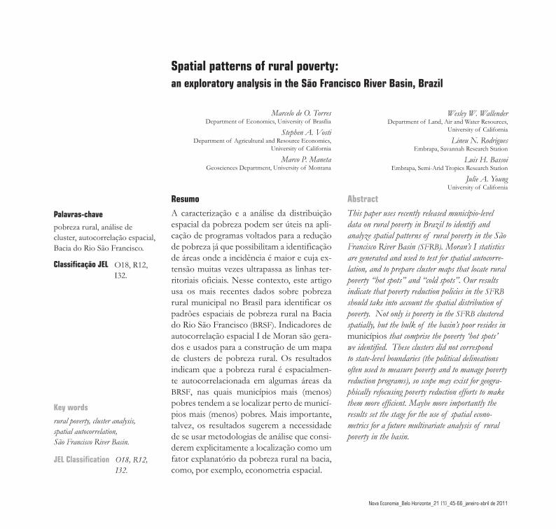
Spatial patterns of rural poverty:an exploratory analysis in the São Francisco River Basin, Brazil

ResumoA caracterização e a análise da distribuição espacial da pobreza podem ser úteis na apli-cação de programas voltados para a redução de pobreza já que possibilitam a identificação de áreas onde a incidência é maior e cuja ex-tensão muitas vezes ultrapassa as linhas ter-ritoriais oficiais. Nesse contexto, este artigo usa os mais recentes dados sobre pobreza rural municipal no Brasil para identificar os padrões espaciais de pobreza rural na Bacia do Rio São Francisco (BRSF). Indicadores de autocorrelação espacial I de Moran são gera-dos e usados para a construção de um mapa de clusters de pobreza rural. Os resultados indicam que a pobreza rural é espacialmen-te autocorrelacionada em algumas áreas da BRSF, nas quais municípios mais (menos) pobres tendem a se localizar perto de municí-pios mais (menos) pobres. Mais importante, talvez, os resultados sugerem a necessidade de se usar metodologias de análise que consi-derem explicitamente a localização como um fator explanatório da pobreza rural na bacia, como, por exemplo, econometria espacial.

AbstractThis paper uses recently released município-level data on rural poverty in Brazil to identify and analyze spatial patterns of rural poverty in the São Francisco River Basin (SFRB). Moran’s I statistics are generated and used to test for spatial autocorre-lation, and to prepare cluster maps that locate rural poverty “hot spots” and “cold spots”. Our results indicate that poverty reduction policies in the SFRB should take into account the spatial distribution of poverty. Not only is poverty in the SFRB clustered spatially, but the bulk of the basin’s poor resides in municípios that comprise the poverty ‘hot spots’ we identified. These clusters did not correspond to state-level boundaries (the political delineations often used to measure poverty and to manage poverty reduction programs), so scope may exist for geogra-phically refocusing poverty reduction efforts to make them more efficient. Maybe more importantly the results set the stage for the use of spatial econo-metrics for a future multivariate analysis of rural poverty in the basin.

Marcelo de O. TorresDepartment of Economics, University of Brasília

Stephen A. VostiDepartment of Agricultural and Resource Economics,

University of California

Marco P. ManetaGeosciences Department, University of Montana

Wesley W. WallenderDepartment of Land, Air and Water Resources,

University of California

Lineu N. RodriguesEmbrapa, Savannah Research Station

Luis H. BassoiEmbrapa, Semi-Arid Tropics Research Station

Julie A. YoungUniversity of California

O18, R12, I32.

O18, R12, I32.

Spatial patterns of rural poverty46


Marcelo de O. Torres_Stephen A. Vosti_Marco P. Maneta_Wesley W. Wallender_Lineu N. Rodrigues_Luis H. Bassoi_Julie A. Young


1_ IntroductionDespite the overall decline in the number of people living in poverty over the past 15 years, approximately 55 million individuals in Brazil remained poor in 2005. Based on the IPEADATA1 database, the percentage of individuals considered poor in Brazil dropped from 42% in 1990 to 31% in 2005. Rural-to-urban migration has accompanied and perhaps fueled this decline in poverty, so with only about 20% of the poor living in rural areas today (Azzoni et al., 2006), poverty in Brazil has become primarily an urban phenomenon. Still, the rural poor should not be neglected, particularly since they are so heavily concentrated in the Northeast of Brazil, where 70% (4.7 million) rural poor and 80% (1.8 million) of the extremely rural poor reside.2

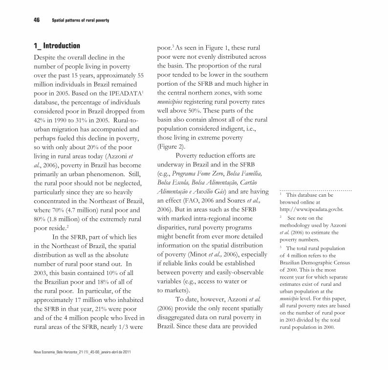
In the SFRB, part of which lies in the Northeast of Brazil, the spatial distribution as well as the absolute number of rural poor stand out. In 2003, this basin contained 10% of all the Brazilian poor and 18% of all of the rural poor. In particular, of the approximately 17 million who inhabited the SFRB in that year, 21% were poor and of the 4 million people who lived in rural areas of the SFRB, nearly 1/3 were

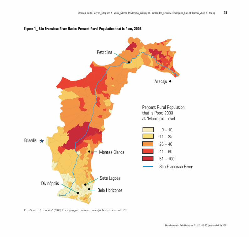
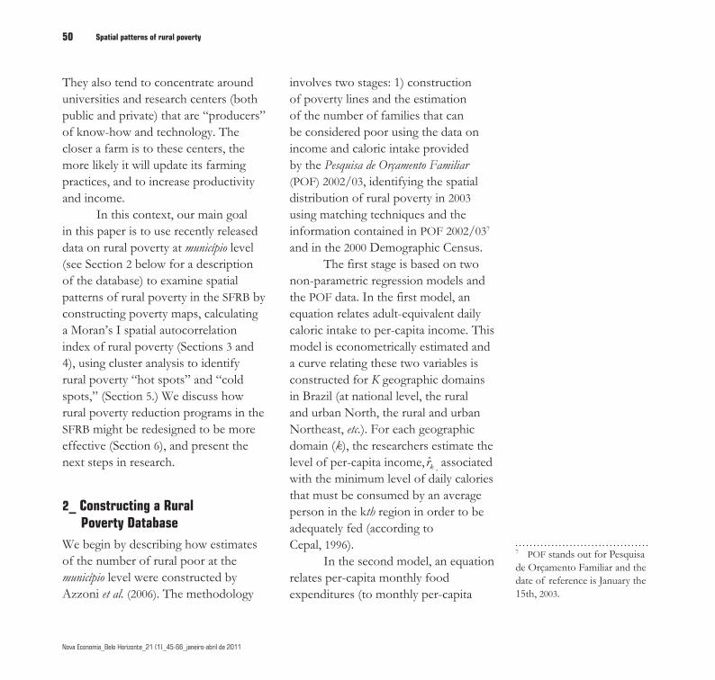
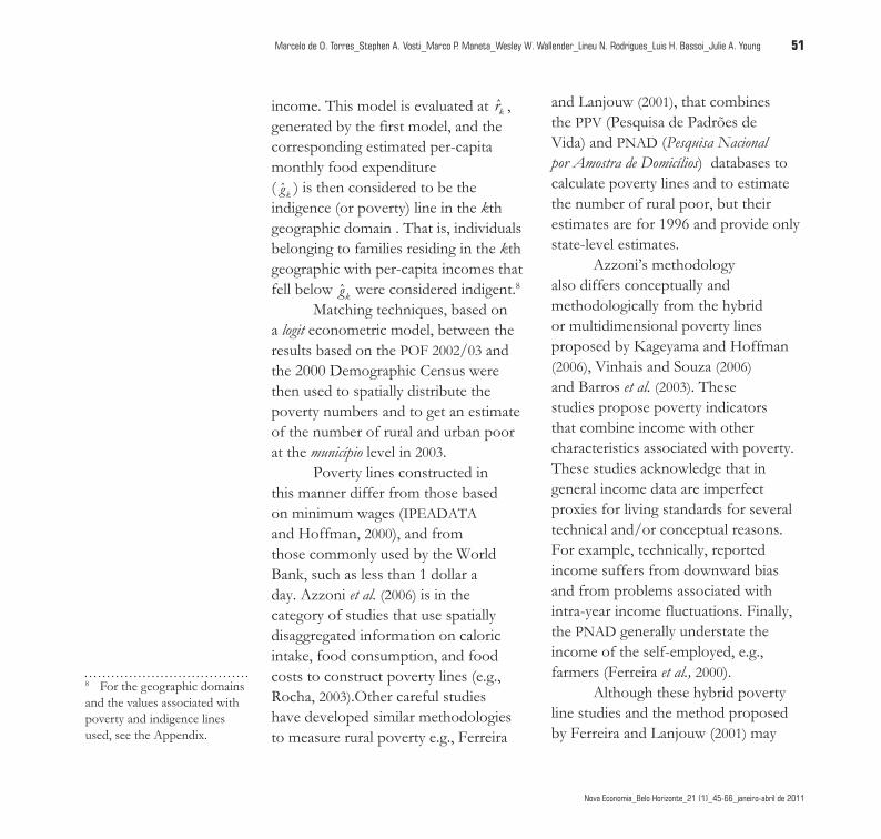
poor.3 As seen in Figure 1, these rural poor were not evenly distributed across the basin. The proportion of the rural poor tended to be lower in the southern portion of the SFRB and much higher in the central northern zones, with some municípios registering rural poverty rates well above 50%. These parts of the basin also contain almost all of the rural population considered indigent, i.e., those living in extreme poverty (Figure 2).

Poverty reduction efforts are underway in Brazil and in the SFRB (e.g., Programa Fome Zero, Bolsa Família, Bolsa Escola, Bolsa Alimentação, Cartão Alimentação e Auxílio Gás) and are having an effect (FAO, 2006 and Soares et al., 2006). But in areas such as the SFRB with marked intra-regional income disparities, rural poverty programs might benefit from ever more detailed information on the spatial distribution of poverty (Minot et al., 2006), especially if reliable links could be established between poverty and easily-observable variables (e.g., access to water or to markets).

To date, however, Azzoni et al. (2006) provide the only recent spatially disaggregated data on rural poverty in Brazil. Since these data are provided

1 This database can be browsed online at http://www.ipeadata.gov.br.2 See note on the methodology used by Azzoni et al. (2006) to estimate the poverty numbers. 3 The total rural population of 4 million refers to the Brazilian Demographic Census of 2000. This is the most recent year for which separate estimates exist of rural and urban population at the município level. For this paper, all rural poverty rates are based on the number of rural poor in 2003 divided by the total rural population in 2000.

Spatial patterns of rural poverty


Marcelo de O. Torres_Stephen A. Vosti_Marco P. Maneta_Wesley W. Wallender_Lineu N. Rodrigues_Luis H. Bassoi_Julie A. Young 47


Figure 1_ São Francisco River Basin: Percent Rural Population that is Poor, 2003

0 – 10

11 – 25

26 – 40

41 – 60

61 – 100

São Francisco River

Sete Lagoas

Montes Claros

Belo HorizonteDivinópolis

Brasília

Petrolina

Aracaju

Percent Rural Populationthat is Poor,at ‘Município’ Level

2003

Data Source: Azzoni et al. (2006). Data aggregated to match município boundaries as of 1991.





Figure 2_ São Francisco River Basin: Percent Rural Population that is Indigent, 2003

Aracaju

0 – 56 – 10

11 – 15

16 – 20

21 – 36

São Francisco River

Sete Lagoas

Montes Claros

Belo HorizonteDivinópolis

Brasília

Petrolina

Percent Rural Populationthat is Indigent,at ‘Município’ Level

2003

Data Source: Azzoni et al. (2006). Data aggregated to match município boundaries as of 1991.





at the município level, it is possible to select the set of municípios within the boundaries of the SFRB4 and construct maps (e.g., Figures 1 and 2) that allow researcher and policymakers to see the distribution of rural poverty across the basin. Such maps are important points of departure, but they leave unanswered key questionings, e.g., can we statistically confirm the spatial patterns that the poverty maps present to us? More specifically, are there rural poverty “hot spots” in the basin, i.e., sub-regions within the SFRB that may have fallen into poverty traps? Or, might there be rural poverty “cold spots” that have successfully escaped poverty and that could provide strategies for doing more generally in the SFRB?

Information on spatial patterns of rural poverty in the SFRB may also shed light on the importance of location as a causal factor per se.5 Municípios may be more likely to have high (low) rural poverty rates depending on where they are located geographically. One obvious reason is the stock of natural resources. For farm activities, we could hardly argue against the fact that good soils and easy access to water may, ceteris paribus, improve agricultural conditions, productivity and income.

Since natural resources are not evenly distributed across space, municípios in favorable areas in terms of natural resources should be more likely to reach higher productivity in agriculture, higher farm income and lower rural poverty rates.

Another reason why location should matter for poverty is that job and income providers such as firms and service-related businesses tend to concentrate in space in order to benefit from larger markets, economies of scale, and external economies of agglomeration such as knowledge spillovers and specialized skilled labor. Rural areas in or close to municípios that happen to have concentrations of such firms and business may benefit from this proximity due to their potential for providing job opportunities (hence income) for non-farm and farm populations.6 This has been highlighted by several authors from the economic geography literature such as Fujita, Krugman and Venables (1999), Fujita and Mori (2005).

These agglomerations of firms and concentration of economic activity usually take place not only in urban centers but in rural towns, as stressed by Haggblade, Hazell and Reardon (2002).

4 See Torres et al. (2006) for an explanation of how municipios ‘falling within’ the SFRB were identified.5 Some recent examples of studies on the link location and poverty are Besley and Burgess (2000), Traxler and Byerlee (2001), Amarasinghe et al. (2005), and Palmer-Jones and Sen (2006).6 For instance, those individuals released from rainfed agricultural activities during the dry season, or from agriculture in general when crop prices fall.





They also tend to concentrate around universities and research centers (both public and private) that are “producers” of know-how and technology. The closer a farm is to these centers, the more likely it will update its farming practices, and to increase productivity and income.

In this context, our main goal in this paper is to use recently released data on rural poverty at município level (see Section 2 below for a description of the database) to examine spatial patterns of rural poverty in the SFRB by constructing poverty maps, calculating a Moran’s I spatial autocorrelation index of rural poverty (Sections 3 and 4), using cluster analysis to identify rural poverty “hot spots” and “cold spots,” (Section 5.) We discuss how rural poverty reduction programs in the SFRB might be redesigned to be more effective (Section 6), and present the next steps in research.

2_ Constructing a Rural Poverty Database We begin by describing how estimates of the number of rural poor at the município level were constructed by Azzoni et al. (2006). The methodology

involves two stages: 1) construction of poverty lines and the estimation of the number of families that can be considered poor using the data on income and caloric intake provided by the Pesquisa de Orçamento Familiar (POF) 2002/03, identifying the spatial distribution of rural poverty in 2003 using matching techniques and the information contained in POF 2002/037 and in the 2000 Demographic Census.

The first stage is based on two non-parametric regression models and the POF data. In the first model, an equation relates adult-equivalent daily caloric intake to per-capita income. This model is econometrically estimated and a curve relating these two variables is constructed for K geographic domains in Brazil (at national level, the rural and urban North, the rural and urban Northeast, etc.). For each geographic domain (k), the researchers estimate the level of per-capita income, k̂r , associated with the minimum level of daily calories that must be consumed by an average person in the kth region in order to be adequately fed (according to Cepal, 1996).

In the second model, an equation relates per-capita monthly food expenditures (to monthly per-capita

7 POF stands out for Pesquisa de Orçamento Familiar and the date of reference is January the 15th, 2003.





income. This model is evaluated at k̂r , generated by the first model, and the corresponding estimated per-capita monthly food expenditure ( ˆkg ) is then considered to be the indigence (or poverty) line in the kth geographic domain . That is, individuals belonging to families residing in the kth geographic with per-capita incomes that fell below ˆkg were considered indigent.8

Matching techniques, based on a logit econometric model, between the results based on the POF 2002/03 and the 2000 Demographic Census were then used to spatially distribute the poverty numbers and to get an estimate of the number of rural and urban poor at the município level in 2003.

Poverty lines constructed in this manner differ from those based on minimum wages (IPEADATA and Hoffman, 2000), and from those commonly used by the World Bank, such as less than 1 dollar a day. Azzoni et al. (2006) is in the category of studies that use spatially disaggregated information on caloric intake, food consumption, and food costs to construct poverty lines (e.g., Rocha, 2003).Other careful studies have developed similar methodologies to measure rural poverty e.g., Ferreira

and Lanjouw (2001), that combines the PPV (Pesquisa de Padrões de Vida) and PNAD (Pesquisa Nacional por Amostra de Domicílios) databases to calculate poverty lines and to estimate the number of rural poor, but their estimates are for 1996 and provide only state-level estimates.

Azzoni’s methodology also differs conceptually and methodologically from the hybrid or multidimensional poverty lines proposed by Kageyama and Hoffman (2006), Vinhais and Souza (2006)and Barros et al. (2003). These studies propose poverty indicators that combine income with other characteristics associated with poverty. These studies acknowledge that in general income data are imperfect proxies for living standards for several technical and/or conceptual reasons. For example, technically, reported income suffers from downward bias and from problems associated with intra-year income fluctuations. Finally, the PNAD generally understate the income of the self-employed, e.g., farmers (Ferreira et al., 2000).

Although these hybrid poverty line studies and the method proposed by Ferreira and Lanjouw (2001) may

8 For the geographic domains and the values associated with poverty and indigence lines used, see the Appendix.





seem comprehensive, they provide poverty numbers at a relatively courser spatial resolution (metropolitan areas or states), which for the study of spatial patterns of rural poverty may be in fact crucial. Data on total poverty (rural and urban combined) from IPEADATA and the Atlas of Human Development 2003 show a significant variation of poverty at the intra-state level (Azzoni’s also demonstrates this). So as highlighted by Helfand (2004) it is important to take into account the considerable heterogeneity in poverty rates within states and/or micro-regions in Brazil.

3_ Spatial Autocorrelation of Rural Poverty in the SFRB – The Moran’s I The main question addressed in this section is whether the observed pattern of rural poverty across the SFRB as seen in Figures 1 and 2 is as equally likely as any other spatial pattern. If we discover, for example, that poor (rich) municípios tended to be surrounded by poor (rich) municípios, or vice-versa, this would indicate there was positive spatial autocorrelation among the rural poor across the basin. If, on the other hand, we find that poor (rich) municípios

tended to be surrounded by rich (poor) municípios, we would then say there was negative spatial autocorrelation among the rural poor across the basin.

To measure spatial autocorrelation, we use the global Moran’s I statistic. Originally developed by Moran (1948), autocorrelation statistics have been extended and applied in several different contexts such as in Cliff and Ord (1981), Anselin (1996), Amarasinghe et al. (2005), Pinkse (2003), Griffith (2003) and Palmer-Jones and Sen (2006), to name a few. In the Brazilian context, it has recently been applied for the analysis of clusters of agricultural productivity (Perobelli et al., 2007).

We begin by defining a proportional measure of rural poverty, i.e., the proportion of the rural population that was poor (p) in each município i, given by

ii

i

np

x=

where ni is the total number of rural poor in município i, and xi is the total rural po-pulation in município i, with i = 1, …, N.

The measure spatial autocorrelation given by the global Moran’s I statistic is defined by

(1)





, ,

2

( )( )/

( ) /

ij i j iji j i j

ii

w p p p p w

Ip p N

− −=

−

∑ ∑∑

where (pi) is rural poverty rate in município i,

ii

pp

N=∑

is the average rural poverty rate over the entire SFRB, and (pj) is the rural poverty rate in município j. The term ( )( )i jp p p p− − is an element of a poverty rate values matrix, with the poverty rates standardized around the sample mean, and wij is a element of a spatial weighting matrix. If município i shares a common boundary with município j, then wij = 1, otherwise wij = 0. This definition of neighboring areas is based on rook contiguity.

In this application, the weighting matrix is row standardized, and the weights are defined as,

ijsij

ijj

ww

w=∑

1sij

j

w =∑, such that

The row standardization has two implications:

i. it implies equal weights across neighbors of a same município;

ii. it implies that the sum over all elements of the row-standardized weight matrix ( s

ijw ) is equal to the total number of observations (N); that is, in (2),

,ij

i j

w N=∑ .11

Therefore, (2) can be re-written as

,

2

( )( )

( )

sij i j

i js

ii

w p p p p

Ip p

− −=

−

∑∑

If municípios with above-average (below-average) poverty rates are surrounded by neighboring municípios with above-average (below-average) poverty rates, the cross product term ( )ip p− ( )jp p− becomes positive, making Is > 0, and implies that there is positive spatial autocorrelation. On the other hand, if municípios with above-average (below-average) poverty rates are surrounded by neighboring municípios with below-average (above-average) poverty rates, the cross product term ( )ip p− ( )jp p− is negative , making Is < 0, and implying that there is negative spatial autocorrelation. The closer Is gets to zero, the weaker the evidence to support spatial autocorrelation.

10

(2’)

.9

9 In the numerator of I,

,

( )( )ij i ji j

w p p p p− −∑ ,

is a gamma statistic with (pi) and (p j ) as random variables, and as such, it is scale-dependent. In order to make it scale-independent, we divide it by

,

iji j

w∑ and by a consistent estimator of the variance of the poverty rate (pi),

2( ) /ii

p p N−∑ .

10 For example, if a município i has 4 neighbors, 1/ 4s

ijw = .11 With row standardization, the sum of weights in each row becomes 1. Since there is one row for each município in the sample, there are N rows. Therefore, the sum over all weights in the matrix,

,

iji j

w∑ , is N.

.





The value of Is calculated using (2’) for all municípios of the SFRB for 2003 is equal to 0.72, which is greater than zero and strongly suggests a positive spatial autocorrelation of rural poverty. 12 Although statistical significance remains to be confirmed, this number suggests that for the SFRB, there are more municípios with high (low) rural poverty rates surrounded by municípios with high (low) rural poverty rates than would be the case that one would expect if poverty were distributed randomly.13 It also indicates that poverty in the SFRB is spatially distributed in clusters, which is compatible with the visual images of the spatial distribution of poverty depicted in Figures 1 and 2, and the notion of contagion or diffusion that suggests that as poverty in neighboring areas increases the likelihood of poverty in its neighbors increases as well (Anselin, 1992). However, this basin-wide statistic does not tell us where these rural poverty clusters might be, but rather only suggests that the spatial pattern of poverty that we observe is not random -- there is more similarity by location than would be expected if the pattern were random.14

4_ Statistical Inference and the Empirical Bayes Index of Spatial AutocorrelationAlthough 0.72 suggests positive spatial autocorrelation of rural poverty, statistical inference analysis is required to statistically confirm this against the null hypothesis of spatial randomness (Ho: Is = 0). To test for the statistical significance of Is, we use an inference procedure based on a permutation approach, in which Is is recomputed for a large number of re-sampled sets of municípios. In each permutation, a Pi is held fixed (not used in the permutation)

12 GeoDaTM is used to calculate all statistics and clusters maps in this paper. This software was developed by the Center for Spatially Integrated Social Science (CSISS) at the University of Illinois, Urbana-Champaign, Urbana, IL, USA. 13 In fact, rural poverty rates are positively spatial autocorrelated for 90% of the municípios in the SFRB; 42% are ‘low-low’, that is, they have below-average rural poverty rates and are surrounded by municípios that have below-average poverty rates; 48% are ‘high-high’, that is, they have above-average rural poverty rates and are

surrounded by municípios that have above-average poverty rates.14 This pattern is consistent when other types of weighting matrices are used. For example, with the contiguity-based Queen weighting matrix the Morans’I is 0.721; using Euclidean Distance Morans’I is 0.652; with a Threshold Distance set to ensure the existence of at least one neighbor for each observation, Morans’I is 0.651; and finally, using the K-Nearest neighbors rule, set at 4 as the number of neighbors for each location, Morans’I is 0.685.





and the remaining poverty rates are re-allocated randomly to the different municípios. For each re-allocation a value for Is is computed. After a given number of permutations, a distribution of Is values is drawn, and a mean and a variance are calculated. This distribution is often called the reference or null distribution (Assunção and Reis, 1999).

One possible problem associated with the permutation approach is that it assumes that any permutation of rural poverty values (pi ) is equally likely to occur among the ( N

) municípios. However, if total rural population differs considerably among the different municípios, those with smaller populations will be more likely to assume extreme values. In other words, the variance of pi may not be constant across municípios and it may in fact increase as the population decreases. As pointed out by Besag and Newell (1991), when this is the case, the null distribution for Is is inaccurate.15

We then follow Assunção and Reis (1999), who propose fixing this problem by adjusting the global Moran’s I as defined in (2’) and correct for the variance instability. Under their approach, ( ip p− ) in (2’) is replaced by ( )iz z− , where

ii

i

p bz

v−

=i

i

zz

N=∑

, and

In (z i ), the mean

ii

ii

nb

x=∑∑

ni is the total number of rural poor individuals in município i, and (xi ) is the total rural population in município i. Also, the variance

ii

bv a

x= +

2

ii

Nba s

x= −

∑in which ,,

22 ( )i i

i ii

x p bs

x−

=∑ ∑and .

Notice that the vi and b are both based on the observed values of population and poverty rates. Notice also that vi now increases as the population xi decreases. By using ( )iz z− , we then redefine (2’) and calculate the so-called EBI – Empirical Bayes Moran’s I (Assunção and Reis, 1999), which in the version with the row-standardized spatial weighting matrix becomes:

12 GeoDaTM is used to calculate all statistics and clusters maps in this paper. This software was developed by the Center for Spatially Integrated Social Science (CSISS) at the University of Illinois, Urbana-Champaign, Urbana, IL, USA. 13 In fact, rural poverty rates are positively spatial autocorrelated for 90% of the municípios in the SFRB; 42% are ‘low-low’, that is, they have below-average rural poverty rates and are surrounded by municípios that have below-average poverty rates; 48% are ‘high-high’, that is, they have above-average rural poverty rates and are

surrounded by municípios that have above-average poverty rates.14 This pattern is consistent when other types of weighting matrices are used. For example, with the contiguity-based Queen weighting matrix the Morans’I is 0.721; using Euclidean Distance Morans’I is 0.652; with a Threshold Distance set to ensure the existence of at least one neighbor for each observation, Morans’I is 0.651; and finally, using the K-Nearest neighbors rule, set at 4 as the number of neighbors for each location, Morans’I is 0.685.

15 Consider, for instance, two municípios (A and B) that are equally poor (say with poverty rates of 50%), and that in location A there are 4 individuals and in B there are 6 individuals. Poor individuals are labeled P, and the non-poor are labeled Np. If 2 individuals are randomly selected from location A, you could draw a sample containing the 2 poor individuals (PP) and conclude that the poverty rate was 100%, or you could draw one poor person and then one non-poor person (PNp) and conclude that the poverty rate was 50%, or a non-poor individual and then a poor one (NpP) and calculate the same 50% rural poverty, or, finally, you could select two non-poor individuals (NpNp) and calculate a rural poverty rate of zero. So, there is a 50% chance of getting the extreme values of 0 and 100% rural poverty. If the same exercise is performed in location B that is comprised of 3 individuals, the odds of getting extreme values of rural poverty is smaller. In more populated location B, the chances of getting the extreme values of 0 and 100% rural poverty drops to half, 1/8 + 1/8 = 25%, as compared with the less-populated location A.

,

(3)





,

2

( )( )

( )

sij i j

i js

ii

w z z z z

EBIz z

− −=

−

∑∑

The next step is to calculate EBIs for the SFRB and use the permutation approach to generate a null distribution, which will then allow us to test for the statistical significance of the measured spatial autocorrelation. We first calculate z i for each of the municípios, and then z . By plugging these values into (4), we find EBIs of 0.83, which confirms the positive spatial autocorrelation of rural poverty rates among the municípios of the SFRB.

The permutation procedure was performed 10,000 times by redistributing the vector of adjusted rural poverty values (z1, z2, z3, … , zN ). Each time the zi values were redistributed, a value for EBIs was calculated. The p-value is calculated as the proportion of times EBIs exceeds 0.83. According to these calculations, the EBIs value of 0.83 is statistically significant at the 5% level of significance, with a standardized Z-value of 25.9 and a p-value = 0.0001.16 This p-value is computed as 1

1MR++

, where R is the number of permutations and M is the number of the statistic computed from the permutations was equal to or greater than 0.83. 17

An EBIs of 0.83 compared with our initial calculation of Moran’s I, Is, of 0.72, indicates that the correlation between rural poverty rates in município i and neighboring municípios is stronger when rates are standardized as in (3) and variance instability is reduced. Hence, increasing the precision with which rural poverty is measured will likely increase the spatial correlation among rural poverty rates in the SFRB.

5_ Local Indicators of Spatial Association (LISA) and Clusters of Rural PovertyAlthough a Moran’s I of 0.83 strongly shows that spatial distribution of rural poverty in the SFRB is not random, it does not locate poverty clusters. We turn to local indicators of spatial association or LISA (Anselin, 1995) for this task. LISA is a class of statistics that provides location-specific information (by município, in this case) and estimates the extent of spatial autocorrelation between the value of a given variable (in our case, rural poverty rate) in a particular location and the values of those same variables in locations around it. Through inference analysis we are able to identify spatial clusters

16 Where [ ]s s

s

I E IZ

VarI

−= . For

the derivation of 1st and 2nd moments of Is , see Cliff and Ord (1981).17 Since the p-value depends on the number of permutations, it is often called pseudo p-value.

(4)





of rural poverty, or rural poverty ‘hot-spots’ (high-poverty municípios surrounded by high-poverty municípios) and/or ‘cold-spots’ (low-poverty municípios surrounded by low-poverty municípios). These clusters might be comprised of a single município and its contiguous neighbors, or a larger set of contiguous municípios for which the LISA is statistically significant. We use the Local Moran’s I statistic or LMI, one of several statistics that falls within the LISA definition.18 It is defined as follows:

2 ,ii ij j

jii

xLMI w x

x= ∑∑

where, i ix p p= − and j jx p p= − , and pi and pj are, respectively, the rural poverty rates for municípios i and j, and p is the sample mean. Spatial

weights, wij, are defined as before: wij = 1 if the i and j municípios are contiguous neighbors, wij = 0 otherwise, based on rook contiguity.

Analogous to the Global Moran’s I, positive values of LMI indicate positive spatial autocorrelation, i.e., that a given município is surrounded by municípios with similar rural poverty rates, either above or below the basin-wide average. On the other hand,

negative values of LMI indicate negative spatial autocorrelation, i.e., that a given município is surrounded by municípios with dissimilar rural poverty rates. If rural poverty is negatively spatially correlated, either a given município with an above-average rural poverty rate is surrounded by neighbors with below-average rural poverty rates, or vice-versa.

We now turn to statistical inference on the LMI. To do so, we use the same procedure employed to test for the significance of the Global Moran’s I. That is, we use the permutation approach in which observed rural poverty rates are randomly re-assigned to each of the municípios. Each time a permutation is performed, a set of N LMIs is calculated; a null distribution for the LMI is constructed and is then used to test for the statistical significance of the observed LMI. We also take into account that the variance of pi is not constant across municípios with different total rural populations, and again follow Assunção and Reis (1999) to adjust the LMI in (4) by substituting iz z− for xi , where zi and z are defined as in Section 3. LMI is then redefined as LEBI or Local Empirical Bayes Moran’s I, (Anselin, 1995):

18 See Anselin (1995) for examples of other LISA statistics, such as the Local Geary.

(5)





2 ( )( )

ii ij j

jii

z zLEBI w z z

z z−

= −− ∑∑

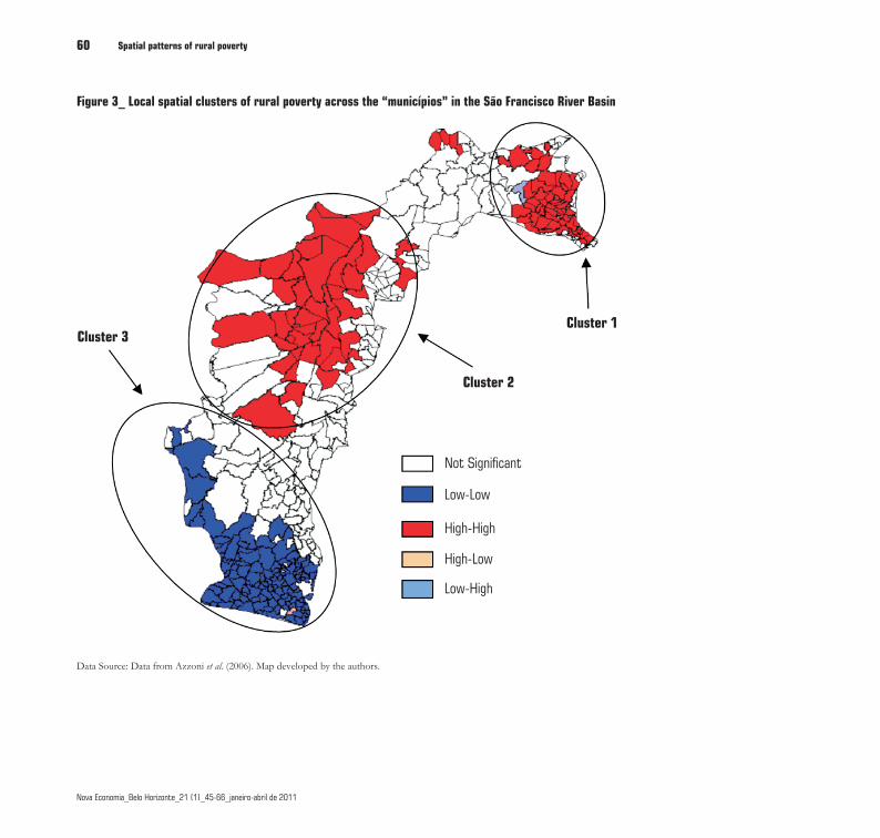
Figure 3 depicts the municípios with statistically significant LEBI, using a significance level of 0.05. We can identify 3 main clusters of rural poverty in the SFRB. Clusters 1 and 2 are rural poverty ‘hot-spots’ and correspond to positive, and high-high spatial autocorrelation, indicating spatial clusters of municípios with above-average rural poverty rates. Cluster 3 is a ‘cold-spot’ and also corresponds to a positive, but low-low, spatial autocorrelation, indicating a spatial cluster of municípios with below-average rural poverty rates. This clearly suggests that there are two spatial autocorrelation patterns of rural poverty values in the São Francisco River Basin. These patterns of rural poverty clustering are different from those based on total poverty (urban and rural) in the same geographic area (Torres et al., 2006). Among other differences, many more clusters of municípios displaying negative autocorrelation (high-low and low-high municípios) were identified when total poverty data were used.

These clusters of rural poverty may be attributable to several reasons.

Although there are obvious candidates for factors that may keep these clusters equally poor (non-poor), such as the lack of irrigation infrastructure in the semi-arid region (which characterizes Cluster 2), or the relatively larger endowments of human capital, agricultural R&D, nearness to major markets (which generally characterize the sub-region occupied Cluster 3), or the extremely low and erratic rainfall and stagnated agriculture systems (which generally characterize the area included in Cluster 1), further analysis is required to determine the causes of these spatial patterns of rural poverty in the SFRB.

For example, in the Brazilian context, though not specific to the SFRB, Helfand and Levine (2004) highlight the role of migration out of rural areas in reducing rural poverty, while others have focused on either demand-side and/or supply-side factors to help explaining spatial patterns of rural poverty in Brazil (e.g., (Jonasson and Helfand, 2009). Ferreira and Lanjouw (2001) highlight the role of education and location of rural communities and farms in relation to urban areas. Helfand (2004) finds evidence of the link between

(6)





rural poverty (on the one hand) and access assets and to markets (on the other). Lastly, Helfand and Del Grossi (2008) show how recent agricultural performance in Brazil has unevenly affected rural poverty and income distribution in Brazil.19

Multivariate regression analysis using the appropriate econometric techniques that take account of spatial interrelationships among poverty rates and the variables that may explain poverty is then the proper analytical approach to the analysis of the spatial determinants of patterns of rural povertyt in the SFRB.

6_ Conclusions and Next StepsIn this paper, we use município-level data to identify and analyze spatial patterns of rural poverty in the São Francisco River Basin (SFRB) in Brazil. We found that rural poverty is spatially autocorrelated in the SFRB – i.e., observed spatial patterns of rural poverty are not likely to be random. More specifically, our results indicate a positive spatial autocorrelation of rural poverty in the SFRB; municípios with

above-average levels of rural poverty tend to be surrounded similarly poor municípios, and municípios with below-average levels of poverty (likewise) tend to be surrounded by similarly better-off municípios.

Looking more deeply into the local patterns of the spatial distribution of rural poverty, we discovered that municípios of the SFRB belonging to Cluster 1 (mainly in the northeastern states of Sergipe and Alagoas in the lower portion of the basin), and to Cluster 2 (mainly northern Minas Gerais and western Bahia) were more likely to have high levels of rural poverty. On the other hand, municípios in the southern portion of the SFRB (those located in relatively high-rainfall areas and closer to large urban centers of Brasília or Belo Horizonte) were more likely to have low levels of rural poverty. Overall, more than 50% of the municípios in the SFRB belonged to one of these three poverty clusters. Roughly half of these municípios were in Clusters 1 or 2, where municípios with above-average poverty rates were surrounded by municípios with above-average poverty rates.

19 For other studies that have examined the determinants of rural poverty in different socioeconomic and agroecological contexts in for example Latin American and Asian countries, see, for example, Finan et al. (2005); Han (2005); Rozelle et al. (2005); Hussain and Hanjra (2004); Besley and Burgess (2000); Fan et al. (2000); Gunning et al. (2000); Scott (2000); Zhang (2000); Blackden and Chitra (1999); Carter and May (1999); Dollar and Kraay (2000); Datt and Ravallion (1998); World Bank (1998); Grootaert et al. (1997); Reardon and Taylor (1996); Binswanger et al. (1995) and Reardon and Vosti (1995).





Figure 3_ Local spatial clusters of rural poverty across the “municípios” in the São Francisco River Basin

Not Significant

Low-Low

High-High

High-Low

Low-High

Cluster 1

Cluster 2

Cluster 3

Data Source: Data from Azzoni et al. (2006). Map developed by the authors.





Our results indicate that poverty reduction policies in the SFRB should take into account the spatial distribution of poverty. Not only is poverty in the SFRB clustered spatially, but the bulk of the basin’s poor resides in municípios that comprise the poverty ‘hot spots’ we identified. These clusters of municípios that comprised poverty ‘hot spots’ did not correspond to state-level boundaries (the political delineations often used to measure poverty and to manage poverty reduction programs), so scope may exist for geographically refocusing poverty reduction efforts to make them more efficient.

Moreover, our analysis suggests that location as a causal factor per se is important and municípios are indeed more likely to have high (low) rural poverty rates depending on where they are located in the basin. This may be due to the obvious reasons such as stock of natural resources, soil quality and access to water which are heterogeneously distributed across the basin. For example we do see that rural poverty tends generally to concentrate in the northern/northeast parts of the basin (see clusters 1 and 2) with notorious problems associated to water access and low agricultural productivity.

But maybe more importantly, our analysis shows that for several reasons, poverty in one município is affected by (or affects) poverty in neighboring municípios. That is, there are spillovers, for example, either positive or negative spatial externalities, that may for example make município more or less likely to get out of poverty.

These spillovers may be associated to the concentration (or lack of) of firms, employment and income in agricultural or non-agricultural sectors, not only in the rural towns of the basin but in urban centers as well. Rural areas in or near neighboring municípios that happen to have concentrations of such firms and businesses (either private or governmental) may benefit from this proximity due to their potential for providing non-farm and farm opportunities and as suppliers of knowledge and technology, for example.

These results set the stage for identifying factors that influence rural poverty in the SFRB, factors that may themselves be spatially correlated. Therefore, our next step is to undertake multivariate spatial econometrics to investigate, among other things:





i. What agroecological factors (e.g., rainfall, topography, soil type) are statistically linked to rural poverty, and if any are linked, how should poverty reduction programs in the SFRB be modified to take these links into consideration?

ii. Why are rural poverty clusters 1 and 2 not contiguous? Are there structural differences between them? What is different about the geographic area that separates the two clusters?

iii. Are there other different and statistically significant types of spatial dependence of rural poverty in the basin, such as spatial error dependence, and how does one take account of such potential differences analytically?





Referências bibliográficas

AMARASINGHE, U.; MADAR, S.; MARKANDU, A. Spatial clustering of rural poverty and food insecurity in Sri Lanka. Food Policy, v. 30, p. 493-509, 2005.

ANSELIN, L. Spatial statistical modeling in a GIS environment. In: MAGUIRE, D.; Goodchild, M.; BATTY, M. (Eds.). GIS, spatial analysis and modeling. Redlands, CA, ESRI Press (forthcoming). [s.d.].

ANSELIN, L. Spatial econometrics: methods and models. Kluwer Academic Publishers: Dordrecht, 1988.

ANSELIN, L. Spatial data analysis with GIS: an introduction to application in the Social Sciences. 1992. (Technical Report 91-10).

ANSELIN, L. Local Indicators of Spatial Association – LISA. Geographical Analysis, v. 27, p. 93-115, 1995.

ANSELIN, L. The Moran Scatterplot as an ESDA Tool to Assess Local Instabil ity in Spatial Association. In: FISCHER, M.; SCHOLTEN, H.; UNWIN, D. (Eds.). Spatial Analytical Perspectives on GIS in Environmental and Socioeconomic Sciences. London: Taylor and Francis, p. 111-125, 1996.

ASSUNÇÃO, R.; REIS, E. A new proposal to adjust Moran’s I for population density. Statistics in Medicine, v. 18, p. 2147-2162, 1999.

AZZONI, C. R.; SILVEIRA, F. G.; CARVALHO, A. Y.; IBARRA, A.; DINIZ, B. P. C.; MOREIRA, G. R. C. Estudo de caracterização e análise da estrutura de consumo e de dispêndio das famílias do meio rural brasileiro: gastos não monetários, auto-consumo e pobreza. 2006. (Relatório final consolidado da espacialização da pobreza no meio rural – Produto 6)

BARROS, R. P. et al. O Índice de Desenvolvimento da Família (IDF). 2003. 20p. (Texto para discussão, n. 986).

BESAG, J.; NEWELL, J. The detection of clusters in rare diseases. Journal of the Royal Statistical Society, v. 154, p. 143-155, 1991.

BESLEY, T.; BURGESS, R. Land reform, poverty reduction and growth: evidence from India. Quarterly Journal of Economics, p. 389-430, 2000.

BINSWANGER, H.; DEININGER, K.; FEDER, G. Power, distortions, revolt, and reform in agricultural land relations. In: BEHRMAN, J.; SRINIVASAN, T. N. (Eds.) Handbook of Development Economics, v. 3B, North-Holland, Amsterdam, 1995.

BLACKDEN, C. M.; CHITRA, B. Gender, growth, and poverty reduction: special program of assistance for África. 1998 status report on poverty in Sub-Saharan Africa. Washington, D.C.: World Bank, 1999. 112 p.

CARTER, M.; MAY, J. Poverty, livelihood and class in rural South Africa. World Development, v. 27, p. 1-20, 1999.

CEPAL. Medición de la pobreza en Brasil: una estimación de las necesidades de energía y proteínas de la población. Santiago, CEPAL, 1996.

CLIFF, A.; ORD, J. Spatial Process: Models and Applications, London: Pion, 1981.

DATT, G.; RAVALLION, M. Why have some Indian states done better than others at reducing rural poverty? Economica, v. 65, p. 17-38, 1998.

DOLLAR, D.; KRAAY, A. Growth is good for the poor. Development Research Group, World Bank, Washington, DC, 2000.

FAN, S.; HAZELL, P.; THORAT, S. government spending, growth and poverty in rural India. American Journal of Agricultural Economics, v. 82, p. 1038-1051, 2000.

FERREIRA, F. H. G.; LANJOUW, P. Rural nonfarm activities and poverty in the Brazilian Northeast. World Development, v. 29, p. 509-528, 2001.

FERREIRA, F. H. G.; LANJOUW, P.; NERI, M. A new poverty profile for Brazil using PPV, PNAD and Census Data. Departamento de Economia, PUC Rio, 2000. (Texto para discussão, n. 418).

FINAN, F.; SADOULET, E.; DE JANVRY, A. Measuring the poverty reduction potential of land in rural Mexico. Journal of Development Economics, v. 77, p. 27-51, 2005.





FOOD and Agriculture Organization (FAO) of the United Nations. Brasil – Fome Zero: Lições Principais. Documento de Trabalho. Escritório Regional da FAO para América Latina e o Caribe, Santiago, Chile. Agosto de 2006.

FUJITA, M.; KRUGMAN, P.; VENABLES, J. The spatial economy: cities, regions and international trade. Cambridge, MA: MIT Press, 1999.

FUJITA, M.; MORI, T. Frontiers of the new economic geography. Institute of Developing Economies, 2005. (Discussion paper, n. 27).

GRIFFITH, D. Spatial autocorrelation and spatial filtering: gaining understanding through theory and scientific visualization. Springer, 2003.

GROOTAERT, C.; KANBUR, R.; GI-TAIK, O. The dynamic of welfare gains and losses: an African case study. Journal of Development Studies, v. 33, p. 635– 657, 1997.

GUNNING, J. W.; HODDINOTT, J.; KINSEY, B.; OWENS, T. Revisiting forever gained: income dynamics in the resettlement areas of Zimbabwe, 1983–96. Journal of Development Studies, v. 36, p. 131-154, 2000.

HAN, H. Rural income poverty in Western China is water poverty source. China & World Economy, v. 13, p. 76, 2005.

HAGGBLADE, S.; HAZELL, P.; REARDOM, T. Strategies for simulating poverty-alleviating growth in the rural nonfarm economy in developing countries. EPDT IFPRI and World Bank, 2002. (Discussion paper, n. 92).

HELFAND, S. M. What can be learned from the agricultural censuses about rural poverty in Brazil? Cuiabá, Mato Grosso, Brazil, 25-28 July, 2004. (Paper prepared for presentation at the conference of the Sociedade Brasileira de Economia e Sociologia Rural – SOBER).

HELFAND, S. M.; DEL GROSSI, M. E. Agricultural boom and rural poverty in Brazil? 1995-2006. FAO, 2008, 61p.

HELFAND, S. M.; LEVINE, E. S. The impact of policy reforms on rural poverty in Brazil: evidence from three states in the 1990’s. In: BOYCE, J. K. et al. (Eds) Human development in the era of globalization: essays in honor of Keith Griffin. 2004.

HOFFMAN, R. Mensuração da desigualdade e pobreza no Brasil. In: HENRIQUES, R. (Ed.). Desiqualdade e pobreza no Brasil. IPEA, 2000.

HUSSAIN, I.;HANJRA, M. A. Irrigation and poverty alleviation: review of the empirical evidence. Irrigation and Drainage, v. 53, p. 1-15, 2004.

IBGE. Brazilian Demographic Census, 2000.

IBGE. POF – Pesquisa de Orçamento Familiar, 2002/2003.

JALAN, J.; RAVALLION, M. Geographic poverty traps? A micro model of consumption growth in rural China. Journal of Applied Economics, v. 17, p. 329-346, 2002.

KAGEYAMA, A.; HOFFMAN, R. Pobreza no Brasil? Uma perspectiva multidimensional. Economia e Sociedade, v. 15, p. 29-112, 2006.

MINOT, N.; BAULCH, B.; EPPRECHT, M. Poverty and Inequality in Vietnam-spatial patterns and Geographic Determinants. International Food Policy Research Institute, 2006. (Paper n. 148).

MORAN, P. The interpretation of statistical maps. Journal of The Royal Statistical Society, v. 10, p. 243-251, 1948.

PALMER-JONES, R.; SEN, K. It is where you are that matters: the spatial determinants of rural poverty in India. Agricultural Economics, v. 34, 2006. p. 229-242.

PEROBELLI, F. S.; ALMEIDA, E. S.; SILVA, M.; FERREIRA, P. G. Produtividade do setor agrícola brasileiro (1991-2003): uma análise espacial, Nova Economia, v. 17, p. 65-91, 2007.

PINKSE, J. Moran-flavored tests with nuisance parameters: examples. In: ANSELIN, L.; FLORAX, R.; REY, S. (Eds.). Advances in spatial econometrics: methodology, tools and applications, Springer, 2003.

RAVALLION, M.; DATT, G. Why has economic growth been more pro-poor in some states in India than others? Journal of Development Economics, v. 68, p. 381-400, 2002.

RAVALLION, M.; JALAN, J. Growth divergences due to spatial externalities. Economic Letters, v. 53, p. 227-232, 1996.

READON, T.; VOSTI, S. Links between rural poverty and the environment in developing countries: asset categories and investment poverty. World Development, v. 23, 1995. p. 1495-1506.

REARDON, T.; TAYLOR, E. J. Agroclimatic shock, income inequality, and poverty: evidence from burkina faso. World Development, v. 24, p. 901-914, 1996.

ROCHA, S. Pobreza no Brasil. Afinal do que se Trata? FGV, 2003.

SCOTT, C. Mixed fortunes: a study of poverty mobility among small farm households in Chile, 1968–1986. Journal of Development Studies, v. 36, p. 155-180, 2000.

SOARES, F. V.; SOARES, S.; MEDRISO, M.; OSÓRIO, R. R. G. Programas de transferência de renda no Brasil? Impactos sobre a desigualdade. IPEA, 2006.(Texto para discussão, n. 1228.





TORRES, M.; VOSTI, S. The distribution of poverty across the São Francisco River Basin: spatial correlations and cluster analysis. São Francisco River Basin Research Team Working Paper, 2006.

TORRES, MARCELO; VOSTI, S. A.; BASSOI, L. H.; HOWITT, R.; MANETA, M.; PFEIFFER, L.; RODRIGUES, L.; WALLENDER, W. W.; YOUNG, J. Identifying the Boundaries of the São Francisco River Basin and the Set of Municípios that Comprise It. São Francisco River Basin Research Team Working Paper, University of California, Davis, July 6, 2006.

TRAXLER, G.; BYERLEE, D. Linking technical change to research effort: an examination of aggregation and spillover effects. Agricutlural Economics, v. 24, p. 235-246, 2001.

UNITED Nations Development Program, IPEA, and Fundação João Pinheiro. Atlas of Human Development in Brazil, 2003.

VINHAIS, H.; SOUZA, A. P. Pobreza relativa ou absoluta? A linha híbrida de pobreza no Brasil. Proceedings of the 34th Brazilian Economics Meeting, 2006.

WANG, J.; XU, Z.; HUANG, J.; ROZELLE, S. Incentives in water management reform:assessing the effect o water use, production, and poverty in the Yellow River Basin. Environmental and Development Economics, v. 10, p. 769-799, 2005.

WORLD BANK. Rural China: transition and development, East Asia and PacificRegion,Washington, DC. World Bank, 1998.

ZHANG, Y. Ten challenges faced with China water resources in the 21stcentury’. Journal of China Water Resources, v. 439, p. 7-8, 2000.

We gratefully acknowledge the financial support provided by the Challenge Program on Water and Food (CPWF) of the Consultative Group on International Agricultural Research (CGIAR), in collaboration with the International Water Management Institute (IWMI). We also gratefully acknowledge financial support from the Center for Natural Resources Policy Analysis (CNRPA) at the University of California, Davis, and the Empresa Brasileira de Pesquisa Agropecuaria (Embrapa). The opinions expressed in this paper are not necessarily those of the supporting agencies.

E-mail de contato dos autores:

[email protected]

Artigo recebido em fevereiro de 2009; aprovado em abril de 2010.



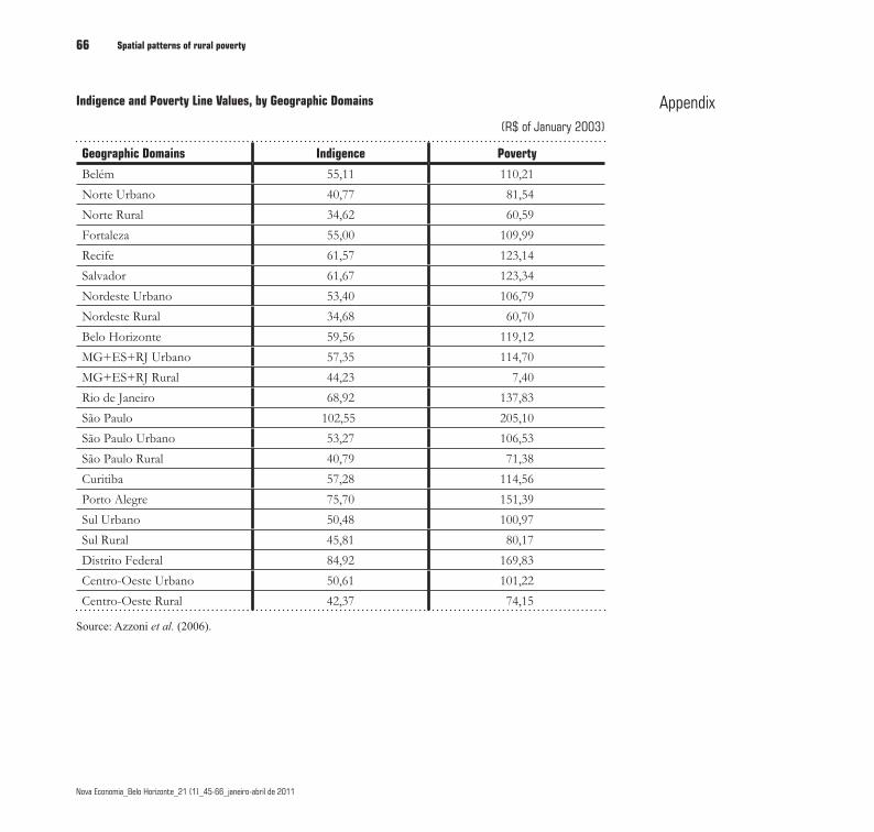
Indigence and Poverty Line Values, by Geographic Domains

(R$ of January 2003)

Geographic Domains Indigence Poverty

Belém 55,11 110,21

Norte Urbano 40,77 81,54

Norte Rural 34,62 60,59

Fortaleza 55,00 109,99

Recife 61,57 123,14

Salvador 61,67 123,34

Nordeste Urbano 53,40 106,79

Nordeste Rural 34,68 60,70

Belo Horizonte 59,56 119,12

MG+ES+RJ Urbano 57,35 114,70

MG+ES+RJ Rural 44,23 7,40

Rio de Janeiro 68,92 137,83

São Paulo 102,55 205,10

São Paulo Urbano 53,27 106,53

São Paulo Rural 40,79 71,38

Curitiba 57,28 114,56

Porto Alegre 75,70 151,39

Sul Urbano 50,48 100,97

Sul Rural 45,81 80,17

Distrito Federal 84,92 169,83

Centro-Oeste Urbano 50,61 101,22

Centro-Oeste Rural 42,37 74,15

Source: Azzoni et al. (2006).

Appendix

Documents

an exploratory analysis in the São Francisco River Basin ... · an exploratory analysis in the São Francisco River Basin, Brazil ... autocorrelação espacial I de Moran são gera-