Improving Software Middleboxes and Datacenter Task Schedulers

IMPROVING SOFTWARE MIDDLEBOXES AND DATACENTERTASK SCHEDULERS

Hugo de Freitas Siqueira Sadok Menna Barreto

Dissertação de Mestrado apresentada aoPrograma de Pós-graduação em EngenhariaElétrica, COPPE, da Universidade Federal doRio de Janeiro, como parte dos requisitosnecessários à obtenção do título de Mestre emEngenharia Elétrica.

Orientadores: Miguel Elias Mitre CampistaLuís Henrique Maciel KosmalskiCosta

Rio de JaneiroOutubro de 2018



DISSERTAÇÃO SUBMETIDA AO CORPO DOCENTE DO INSTITUTOALBERTO LUIZ COIMBRA DE PÓS-GRADUAÇÃO E PESQUISA DEENGENHARIA (COPPE) DA UNIVERSIDADE FEDERAL DO RIO DEJANEIRO COMO PARTE DOS REQUISITOS NECESSÁRIOS PARA AOBTENÇÃO DO GRAU DE MESTRE EM CIÊNCIAS EM ENGENHARIAELÉTRICA.

Examinada por:

Prof. Miguel Elias Mitre Campista, D.Sc.

Prof. Otto Carlos Muniz Bandeira Duarte, Dr.Ing.

Prof. Artur Ziviani, Dr.

Prof. Ítalo Fernando Scotá Cunha, Dr.

RIO DE JANEIRO, RJ – BRASILOUTUBRO DE 2018

Barreto, Hugo de Freitas Siqueira Sadok MennaImproving Software Middleboxes and Datacenter

Task Schedulers/Hugo de Freitas Siqueira Sadok MennaBarreto. – Rio de Janeiro: UFRJ/COPPE, 2018.

XV, 69 p.: il.; 29, 7cm.Orientadores: Miguel Elias Mitre Campista

Luís Henrique Maciel Kosmalski CostaDissertação (mestrado) – UFRJ/COPPE/Programa de

Engenharia Elétrica, 2018.Referências Bibliográficas: p. 59 – 69.1. Middleboxes. 2. Task Schedulers. 3.

Fairness. I. Campista, Miguel Elias Mitre et al.II. Universidade Federal do Rio de Janeiro, COPPE,Programa de Engenharia Elétrica. III. Título.

iii

To my parents and grandmother.

iv

Agradecimentos

Muitas pessoas contribuíram para esta dissertação de forma direta ou indireta. Aseguir há uma tentativa de agradecer a elas.

Primeiro agradeço aos meus pais Marcelo e Márcia Sadok, e à minha vó CarmenSiqueira, por sempre acreditarem em mim e por me darem suporte incondicional.Sem eles nada disso seria possível. Agradeço também aos meus irmãos Bruno e LunaSadok. Bruno por aturar minhas piadas inoportunas, pelas excelentes conversas epor até mesmo revisar alguns textos (chatos segundo ele). Luna por jogar comigo epelos desenhos mais legais que já recebi.

Esta dissertação também não existiria se não fossem os meus orientadores MiguelCampista e Luís Costa. Eles me orientaram desde a graduação e me deram liberdadepara trabalhar nos problemas que eu mais gostava—por mais ecléticos que fossem.Sou muito grato por terem me introduzido à pesquisa em redes de computadorese por todos os ensinamentos que recebi nesses anos (como fazer pesquisa, comoescrever, como apresentar, etc.).

Além dos meus orientadores sou grato aos demais professores do GTA. Agradeçoao Otto Duarte, pelas palavras de sabedoria, alegorias, por aceitar fazer parte dabanca e pelas críticas valiosas durante a defesa; ao Pedro Velloso, por ter sido maiscolega do que professor; e ao Rodrigo Couto, por ter me ajudado muito desde quandoentrei no GTA.

Meus agradecimentos também vão para os demais membros e ex-membros doGTA. Em especial para o Pedro Cruz, Fernando Molano, Dianne Medeiros eLeopoldo Mauricio. O Pedro não cansou de dar inúmeras sugestões nos momen-tos em que eu empacava, e não cansou de receber meus inúmeros pitacos quandoele era o empacado. O Molano é uma das pessoas mais solícitas que já conheci etambém me ajudou incontáveis vezes. A Dianne foi minha colega de sala por boaparte do mestrado e me deu várias lições valiosas. Finalmente o Leopoldo, mesmosendo aluno parcial, me ajudou a conseguir máquinas para simulação em momentode desespero e me forneceu uma visão prática de alguns dos temas desta dissertação.Agradeço também ao Antonio Silvério, Diogo Mattos, Eric Oliveira, Edvar Afonso,Igor Sanz, Lucas Gomes, Mariana Maciel, Martin Andreoni e Thales Almeida.

Fora do GTA, agradeço aos professores Daniel Figueiredo, José Gabriel Gomes

v

e Valmir Barbosa pelas excelentes aulas, e aos professores Artur Ziviani e ÍtaloCunha por terem aceitado fazer parte da banca e pelas excelentes críticas e sugestõesdurante a defesa.

O presente trabalho foi realizado com apoio da Coordenação de Aperfeiçoamentode Pessoal de Nível Superior – Brasil (CAPES) – Código de Financiamento 001.Além disso este trabalho contou com apoio do Conselho Nacional de Desenvolvi-mento Científico e Tecnológico (CNPq), da Fundação de Amparo à Pesquisa doEstado do Rio de Janeiro (FAPERJ), e da Fundação de Amparo à Pesquisa doEstado de São Paulo (FAPESP), processos #15/24494-8 e #15/24490-2.

vi

Resumo da Dissertação apresentada à COPPE/UFRJ como parte dos requisitosnecessários para a obtenção do grau de Mestre em Ciências (M.Sc.)

APRIMORANDO MIDDLEBOXES EM SOFTWARE E ESCALONADORESDE TAREFAS DE DATACENTERS


Outubro/2018

Orientadores: Miguel Elias Mitre CampistaLuís Henrique Maciel Kosmalski Costa

Programa: Engenharia Elétrica

Nas últimas décadas, sistemas compartilhados contribuíram para a popularidadede muitas tecnologias. Desde Sistemas Operacionais até a Internet, esses sistemastrouxeram economias significativas ao permitir que a infraestrutura subjacente fossecompartilhada. Um desafio comum a esses sistemas é garantir que os recursos sejamdivididos de forma justa, sem comprometer a eficiência de utilização. Esta disserta-ção observa problemas em dois sistemas compartilhados distintos—middleboxes emsoftware e escalonadores de tarefas de datacenters—e propõe maneiras de melhorartanto a eficiência como a justiça. Primeiro é apresentado o sistema Sprayer, queusa espalhamento para direcionar pacotes entre os núcleos em middleboxes em soft-ware. O Sprayer elimina os problemas de desbalanceamento causados pelas soluçõesbaseadas em fluxos e lida com os novos desafios de manipular estados de fluxo, con-sequentes do espalhamento de pacotes. É mostrado que o Sprayer melhora a justiçade forma significativa e consegue usar toda a capacidade, mesmo quando há apenasum fluxo no sistema. Depois disso, é apresentado o SDRF, uma política de alocaçãode tarefas para datacenters que considera as alocações passadas e garante justiça aolongo do tempo. Prova-se que o SDRF mantém as propriedades fundamentais doDRF—a política de alocação em que ele se baseia—enquanto beneficia os usuárioscom menor utilização. Para implementar o SDRF de forma eficiente, também éintroduzida a árvore viva, uma estrutura de dados genérica que mantém ordenadoselementos cujas prioridades variam com o tempo. Simulações com dados reais in-dicam que o SDRF reduz o tempo de espera na média. Isso melhora a justiça, aoaumentar o número de tarefas completas dos usuários com menor demanda, tendoum impacto pequeno nos usuários de maior demanda.

vii

Abstract of Dissertation presented to COPPE/UFRJ as a partial fulfillment of therequirements for the degree of Master of Science (M.Sc.)



October/2018

Advisors: Miguel Elias Mitre CampistaLuís Henrique Maciel Kosmalski Costa

Department: Electrical Engineering

Over the last decades, shared systems have contributed to the popularity ofmany technologies. From Operating Systems to the Internet, they have all broughtsignificant cost savings by allowing the underlying infrastructure to be shared. Acommon challenge in these systems is to ensure that resources are fairly dividedwithout compromising utilization efficiency. In this thesis, we look at problemsin two shared systems—software middleboxes and datacenter task schedulers—andpropose ways of improving both efficiency and fairness. We begin by presentingSprayer, a system that uses packet spraying to load balance packets to cores in soft-ware middleboxes. Sprayer eliminates the imbalance problems of per-flow solutionsand addresses the new challenges of handling shared flow state that come with packetspraying. We show that Sprayer significantly improves fairness and seamlessly usesthe entire capacity, even when there is a single flow in the system. After that, wepresent Stateful Dominant Resource Fairness (SDRF), a task scheduling policy fordatacenters that looks at past allocations and enforces fairness in the long run. Weprove that SDRF keeps the fundamental properties of DRF—the allocation policyit is built on—while benefiting users with lower usage. To efficiently implementSDRF, we also introduce live tree, a general-purpose data structure that keeps ele-ments with predictable time-varying priorities sorted. Our trace-driven simulationsindicate that SDRF reduces users’ waiting time on average. This improves fairness,by increasing the number of completed tasks for users with lower demands, withsmall impact on high-demand users.

viii

Contents

List of Figures xi

List of Tables xiii

List of Abbreviations xiv

1 Introduction 11.1 Efficient Use of Multiple Cores in Software Middleboxes . . . . . . . . 21.2 Improving Datacenter Scheduling by Considering Long-Term Fairness 31.3 Outline . . . . . . . . . . . . . . . . . . . . . . . . . . . . . . . . . . 4

2 Background 52.1 Middleboxes and the Move to Software . . . . . . . . . . . . . . . . . 5

2.1.1 The Move to Software . . . . . . . . . . . . . . . . . . . . . . 62.1.2 Packet Processing on x86 . . . . . . . . . . . . . . . . . . . . 62.1.3 Using Multiple CPU Cores . . . . . . . . . . . . . . . . . . . . 9

2.2 Datacenter Task Scheduling . . . . . . . . . . . . . . . . . . . . . . . 102.2.1 Resource Allocation . . . . . . . . . . . . . . . . . . . . . . . 102.2.2 Multiple Resource Types . . . . . . . . . . . . . . . . . . . . . 11

3 Sprayer 133.1 Motivation . . . . . . . . . . . . . . . . . . . . . . . . . . . . . . . . . 133.2 Design . . . . . . . . . . . . . . . . . . . . . . . . . . . . . . . . . . . 15

3.2.1 How to spray packets? . . . . . . . . . . . . . . . . . . . . . . 153.2.2 How to handle flow state? . . . . . . . . . . . . . . . . . . . . 163.2.3 Architecture . . . . . . . . . . . . . . . . . . . . . . . . . . . . 173.2.4 Programming Model . . . . . . . . . . . . . . . . . . . . . . . 18

3.3 Implementation . . . . . . . . . . . . . . . . . . . . . . . . . . . . . . 193.4 Evaluation . . . . . . . . . . . . . . . . . . . . . . . . . . . . . . . . . 213.5 Discussion . . . . . . . . . . . . . . . . . . . . . . . . . . . . . . . . . 243.6 Related Work . . . . . . . . . . . . . . . . . . . . . . . . . . . . . . . 253.7 Conclusion . . . . . . . . . . . . . . . . . . . . . . . . . . . . . . . . . 26

ix

4 Stateful Dominant Resource Fairness 274.1 System Model . . . . . . . . . . . . . . . . . . . . . . . . . . . . . . . 28

4.1.1 Multi-Resource Setting and Allocation Mechanism . . . . . . 284.1.2 Repeated Game . . . . . . . . . . . . . . . . . . . . . . . . . . 29

4.2 DRF and Allocation Properties . . . . . . . . . . . . . . . . . . . . . 294.2.1 DRF Mechanism . . . . . . . . . . . . . . . . . . . . . . . . . 304.2.2 Static Allocation Properties . . . . . . . . . . . . . . . . . . . 314.2.3 Fairness in the Dynamic Setting . . . . . . . . . . . . . . . . . 324.2.4 Users’ Commitments . . . . . . . . . . . . . . . . . . . . . . . 33

4.3 Stateful Dominant Resource Fairness . . . . . . . . . . . . . . . . . . 334.3.1 Stateful Max-Min Fairness . . . . . . . . . . . . . . . . . . . . 334.3.2 SDRF Mechanism . . . . . . . . . . . . . . . . . . . . . . . . 354.3.3 Analysis of SDRF Allocation Properties . . . . . . . . . . . . 36

4.4 Implementation Using a Live Tree . . . . . . . . . . . . . . . . . . . . 374.4.1 Continuous Time . . . . . . . . . . . . . . . . . . . . . . . . . 374.4.2 Indivisible Tasks . . . . . . . . . . . . . . . . . . . . . . . . . 384.4.3 Live Tree . . . . . . . . . . . . . . . . . . . . . . . . . . . . . 394.4.4 Live Tree Applied to SDRF . . . . . . . . . . . . . . . . . . . 42

4.5 Simulation Results . . . . . . . . . . . . . . . . . . . . . . . . . . . . 434.6 Related Work . . . . . . . . . . . . . . . . . . . . . . . . . . . . . . . 464.7 Conclusion . . . . . . . . . . . . . . . . . . . . . . . . . . . . . . . . . 474.8 Deferred Proofs . . . . . . . . . . . . . . . . . . . . . . . . . . . . . . 48

5 Conclusions and the Future of Networks and Datacenters 565.1 Domain-Specific Architectures . . . . . . . . . . . . . . . . . . . . . . 575.2 Decentralized Control and Computation . . . . . . . . . . . . . . . . 57

Bibliography 59

x

List of Figures

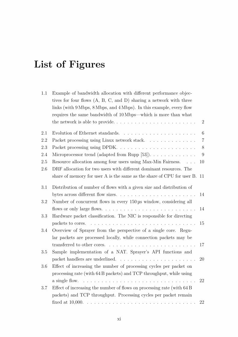
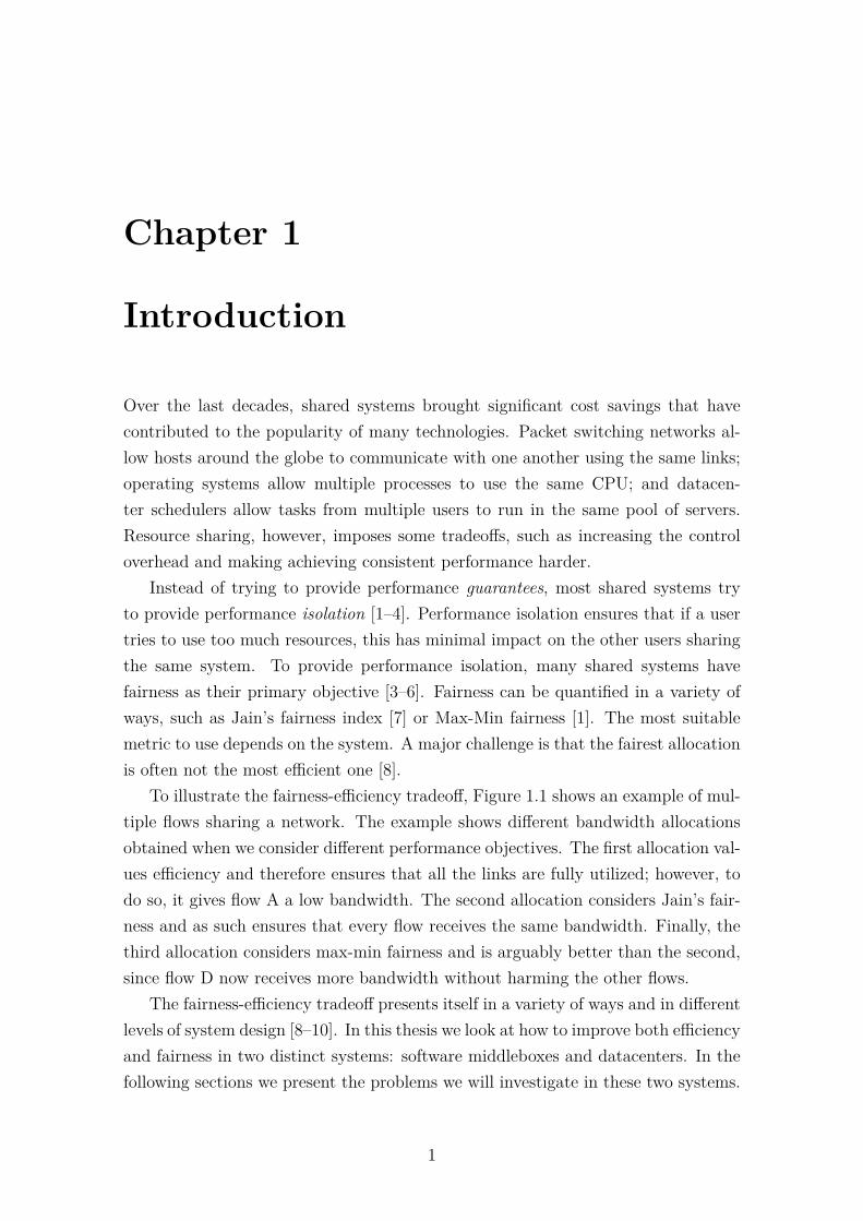
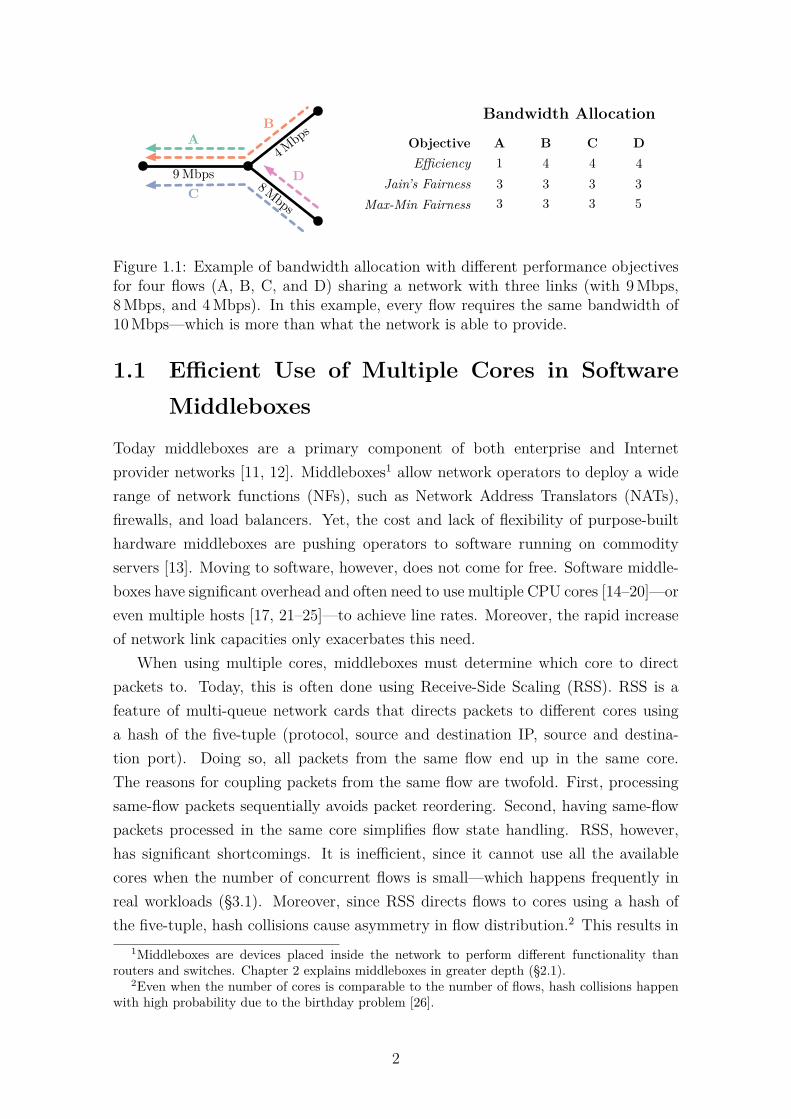
1.1 Example of bandwidth allocation with different performance objec-tives for four flows (A, B, C, and D) sharing a network with threelinks (with 9 Mbps, 8 Mbps, and 4 Mbps). In this example, every flowrequires the same bandwidth of 10 Mbps—which is more than whatthe network is able to provide. . . . . . . . . . . . . . . . . . . . . . . 2

2.1 Evolution of Ethernet standards. . . . . . . . . . . . . . . . . . . . . 62.2 Packet processing using Linux network stack. . . . . . . . . . . . . . 72.3 Packet processing using DPDK. . . . . . . . . . . . . . . . . . . . . . 82.4 Microprocessor trend (adapted from Rupp [53]). . . . . . . . . . . . . 92.5 Resource allocation among four users using Max-Min Fairness. . . . 102.6 DRF allocation for two users with different dominant resources. The

share of memory for user A is the same as the share of CPU for user B. 11

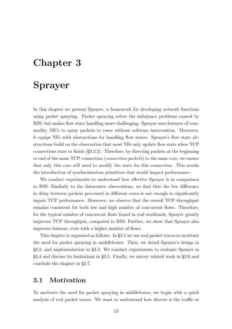
3.1 Distribution of number of flows with a given size and distribution ofbytes across different flow sizes. . . . . . . . . . . . . . . . . . . . . . 14

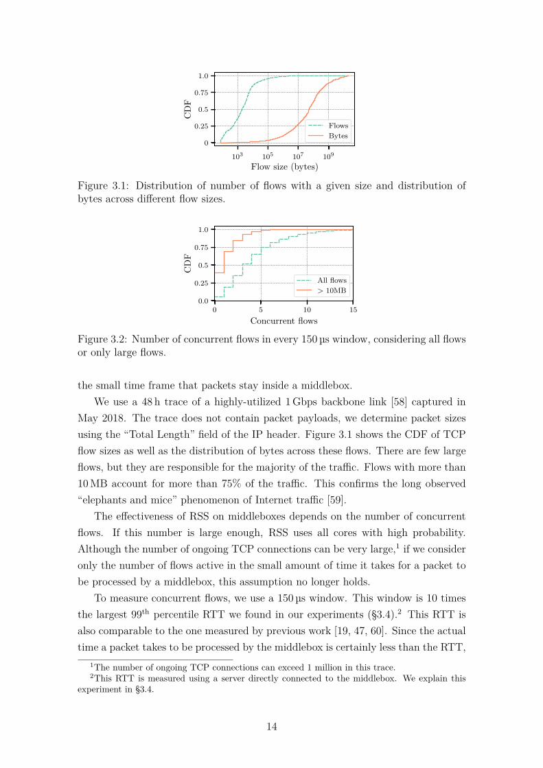
3.2 Number of concurrent flows in every 150 µs window, considering allflows or only large flows. . . . . . . . . . . . . . . . . . . . . . . . . . 14

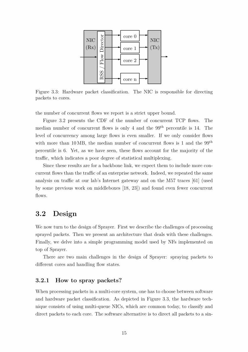
3.3 Hardware packet classification. The NIC is responsible for directingpackets to cores. . . . . . . . . . . . . . . . . . . . . . . . . . . . . . 15

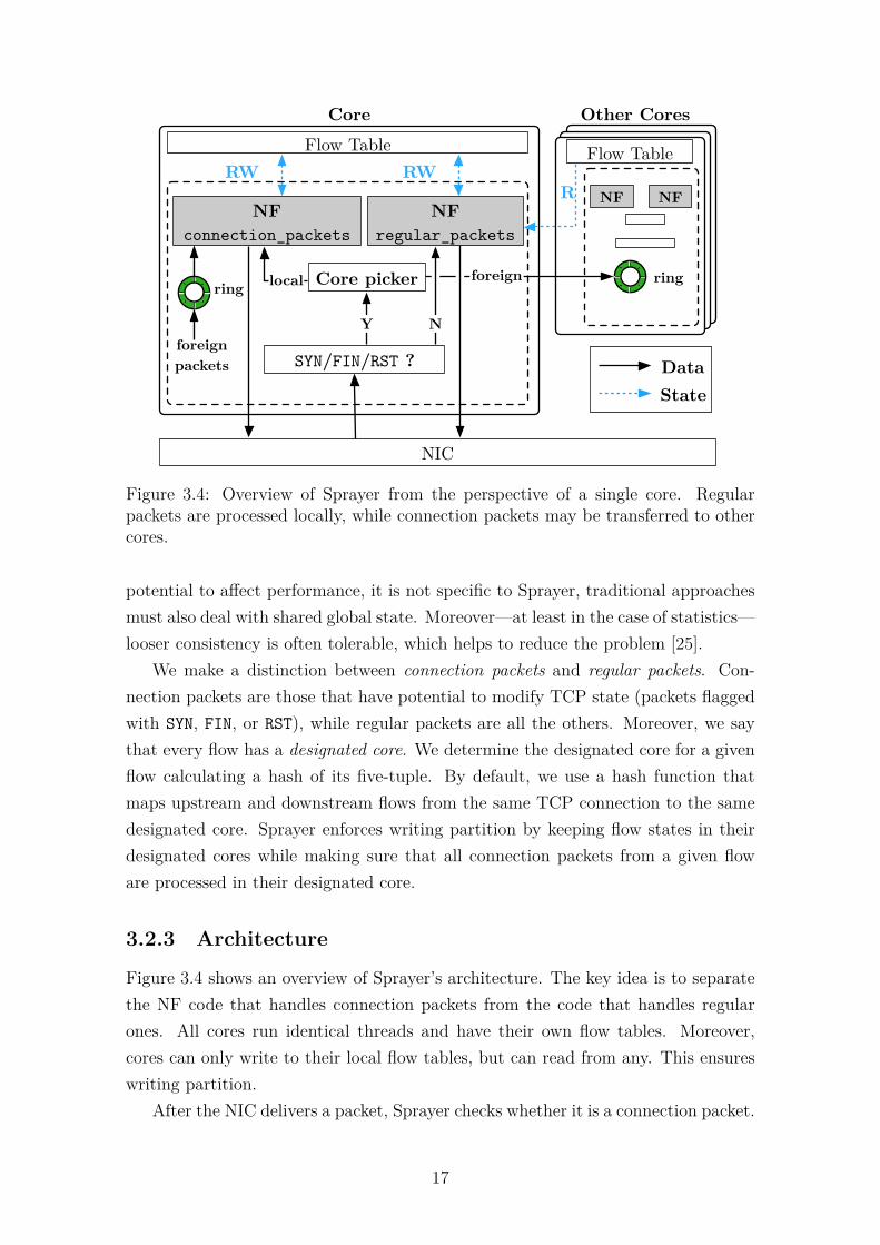
3.4 Overview of Sprayer from the perspective of a single core. Regu-lar packets are processed locally, while connection packets may betransferred to other cores. . . . . . . . . . . . . . . . . . . . . . . . . 17

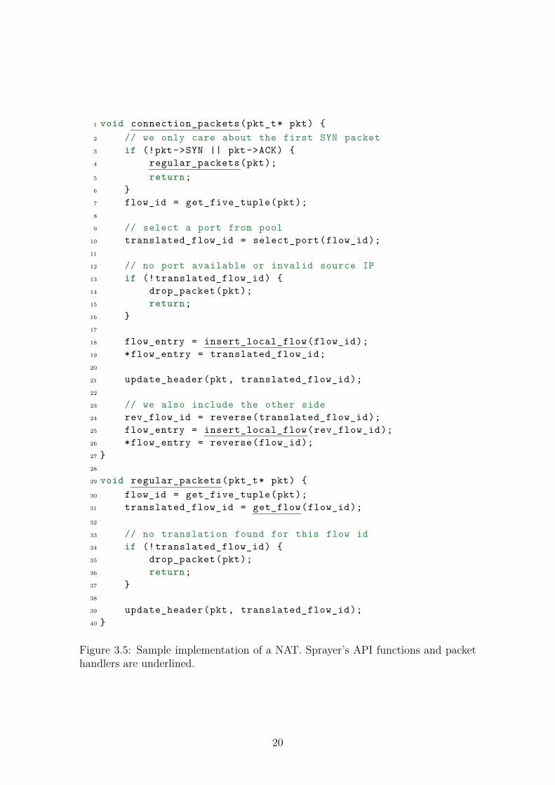
3.5 Sample implementation of a NAT. Sprayer’s API functions andpacket handlers are underlined. . . . . . . . . . . . . . . . . . . . . . 20

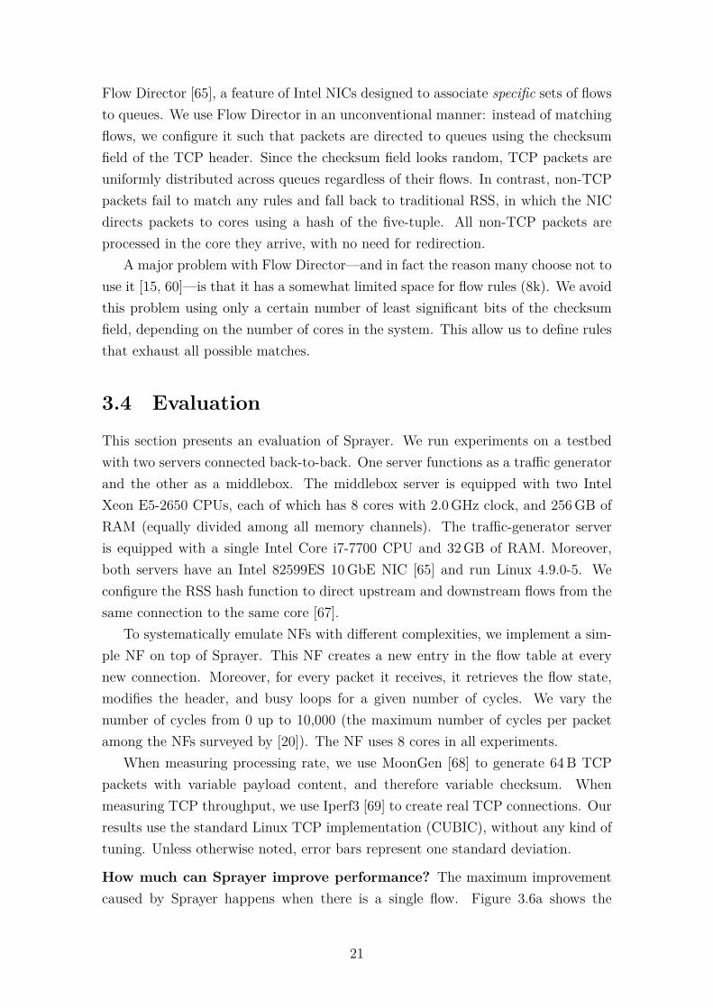
3.6 Effect of increasing the number of processing cycles per packet onprocessing rate (with 64 B packets) and TCP throughput, while usinga single flow. . . . . . . . . . . . . . . . . . . . . . . . . . . . . . . . 22

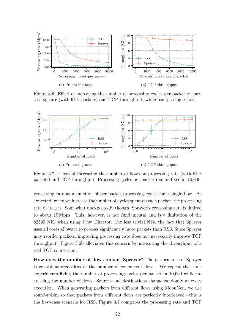
3.7 Effect of increasing the number of flows on processing rate (with 64 Bpackets) and TCP throughput. Processing cycles per packet remainfixed at 10,000. . . . . . . . . . . . . . . . . . . . . . . . . . . . . . . 22

xi

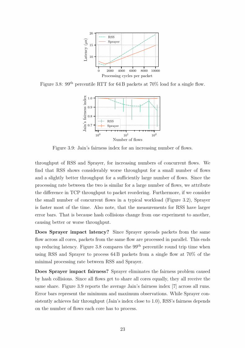
3.8 99th percentile RTT for 64 B packets at 70% load for a single flow. . . 233.9 Jain’s fairness index for an increasing number of flows. . . . . . . . . 23

4.1 Unfairness in the long run. User B hardly uses the system but receivesthe same shares as user A. . . . . . . . . . . . . . . . . . . . . . . . . 32

4.2 Water-filling diagram for (a) MMF and (b) SMMF. . . . . . . . . . . 344.3 Illustration of a live tree with its data structures. Positions in the

array link to elements in the tree. Some elements link to events inthe events tree. . . . . . . . . . . . . . . . . . . . . . . . . . . . . . . 39

4.4 Example of insertion: Insert(4, κ4). . . . . . . . . . . . . . . . . . . 404.5 Example of event update: UpdateEvent(3). . . . . . . . . . . . . . 404.6 Example of time update: Update(t). . . . . . . . . . . . . . . . . . . 414.7 Example of deletion: Delete(3). . . . . . . . . . . . . . . . . . . . . 414.8 Same example as Figure 4.1 but using SDRF (δ = 1−10−6). Note how

user B receives more resources and is able to complete her workloadfaster. . . . . . . . . . . . . . . . . . . . . . . . . . . . . . . . . . . . 44

4.9 Mean wait time reduction for every user relative to DRF. . . . . . . . 444.10 Task completion ratio using DRF and SDRF. Each bubble is a dif-

ferent user. The bubble’s size is logarithmic to the number of taskssubmitted by the user. Users above the y = x are better with SDRF. 45

4.11 Live tree events for different values of discount factor and systemresources (50% to 100% of R from top to bottom). . . . . . . . . . . 46

xii

List of Tables

3.1 Example of state scope and access pattern of some popular statefulNFs. Most NFs only update flow states when connections start orfinish. . . . . . . . . . . . . . . . . . . . . . . . . . . . . . . . . . . . 16

3.2 Flow state API. . . . . . . . . . . . . . . . . . . . . . . . . . . . . . . 18

4.1 Summary of notations. . . . . . . . . . . . . . . . . . . . . . . . . . . 30

xiii

List of Abbreviations

ACL Access Control List, p. 24

API Application Programming Interface, p. 9

ASIC Application-Specific Integrated Circuit, p. 57

BMF Bottleneck Max Fairness, p. 47

CDF Cumulative Distribution Function, p. 14

CPU Central Processing Unit, p. 1

DDIO Data Direct I/O, p. 9

DMA Direct Memory Access, p. 7

DPDK Data Plane Development Kit, p. 8

DPI Deep Packet Inspection, p. 5, 16

DRF Dominant Resource Fairness, p. 3, 11, 30

DSA Domain-Specific Architecture, p. 57

DSO Distributed Shared Object, p. 25

ECMP Equal Cost Multi-Path, p. 3

FIN TCP flag to indicate the last packet from a sender, p. 17

GPU Graphics Processing Unit, p. 57

GTA Teleinformatics and Automation Group (Grupo de Teleinfor-mática e Automação), p. v

I/O Input/Output, p. 3

IP Internet Protocol, p. 5

IPv4 Internet Protocol, version 4, p. 5

xiv

IPv6 Internet Protocol, version 6, p. 5

MMF Max-Min Fairness, p. 10, 30, 34

NAT Network Address Translator, p. 2, 5

NFV Network Function Virtualization, p. 6

NF Network Function, p. 2, 6

NIC Network Interface Controller, p. 7

OS Operating System, p. 7

PO Pareto Optimality, p. 31

QUIC Quick UDP Internet Connection, p. 25

RAM Random-access Memory, p. 21

RFC Request for Comments, p. 5

RSS Receive-Side Scaling, p. 2, 9

RST TCP flag to reset the connection, p. 17

RTT Round-Trip Time, p. 14

SDRF Stateful Dominant Resource Fairness, p. 27, 33

SI Sharing Incentives, p. 31

SMMF Stateful Max-Min Fairness, p. 34

SP Strategyproofness, p. 31

SQL Structured Query Language, p. 10

SYN TCP flag to synchronize sequence numbers, p. 17

TCP Transmission Control Protocol, p. 3

TPU Tensor Processing Unit, p. 57

UDP User Datagram Protocol, p. 25

UIO User-space I/O, p. 8

VoIP Voice over IP, p. 25

YARN Yet Another Resource Negotiator, p. 10

xv

Chapter 1

Introduction

Over the last decades, shared systems brought significant cost savings that havecontributed to the popularity of many technologies. Packet switching networks al-low hosts around the globe to communicate with one another using the same links;operating systems allow multiple processes to use the same CPU; and datacen-ter schedulers allow tasks from multiple users to run in the same pool of servers.Resource sharing, however, imposes some tradeoffs, such as increasing the controloverhead and making achieving consistent performance harder.

Instead of trying to provide performance guarantees, most shared systems tryto provide performance isolation [1–4]. Performance isolation ensures that if a usertries to use too much resources, this has minimal impact on the other users sharingthe same system. To provide performance isolation, many shared systems havefairness as their primary objective [3–6]. Fairness can be quantified in a variety ofways, such as Jain’s fairness index [7] or Max-Min fairness [1]. The most suitablemetric to use depends on the system. A major challenge is that the fairest allocationis often not the most efficient one [8].

To illustrate the fairness-efficiency tradeoff, Figure 1.1 shows an example of mul-tiple flows sharing a network. The example shows different bandwidth allocationsobtained when we consider different performance objectives. The first allocation val-ues efficiency and therefore ensures that all the links are fully utilized; however, todo so, it gives flow A a low bandwidth. The second allocation considers Jain’s fair-ness and as such ensures that every flow receives the same bandwidth. Finally, thethird allocation considers max-min fairness and is arguably better than the second,since flow D now receives more bandwidth without harming the other flows.

The fairness-efficiency tradeoff presents itself in a variety of ways and in differentlevels of system design [8–10]. In this thesis we look at how to improve both efficiencyand fairness in two distinct systems: software middleboxes and datacenters. In thefollowing sections we present the problems we will investigate in these two systems.

1

Efficiency

CD

BA

9 Mbps4 M

bps

8 MbpsJain’s Fairness

Max-Min Fairness

A B C D1 4 4 43 3 3 33 3 3 5

Bandwidth AllocationObjective

Figure 1.1: Example of bandwidth allocation with different performance objectivesfor four flows (A, B, C, and D) sharing a network with three links (with 9 Mbps,8 Mbps, and 4 Mbps). In this example, every flow requires the same bandwidth of10 Mbps—which is more than what the network is able to provide.

1.1 Efficient Use of Multiple Cores in SoftwareMiddleboxes

Today middleboxes are a primary component of both enterprise and Internetprovider networks [11, 12]. Middleboxes1 allow network operators to deploy a widerange of network functions (NFs), such as Network Address Translators (NATs),firewalls, and load balancers. Yet, the cost and lack of flexibility of purpose-builthardware middleboxes are pushing operators to software running on commodityservers [13]. Moving to software, however, does not come for free. Software middle-boxes have significant overhead and often need to use multiple CPU cores [14–20]—oreven multiple hosts [17, 21–25]—to achieve line rates. Moreover, the rapid increaseof network link capacities only exacerbates this need.

When using multiple cores, middleboxes must determine which core to directpackets to. Today, this is often done using Receive-Side Scaling (RSS). RSS is afeature of multi-queue network cards that directs packets to different cores usinga hash of the five-tuple (protocol, source and destination IP, source and destina-tion port). Doing so, all packets from the same flow end up in the same core.The reasons for coupling packets from the same flow are twofold. First, processingsame-flow packets sequentially avoids packet reordering. Second, having same-flowpackets processed in the same core simplifies flow state handling. RSS, however,has significant shortcomings. It is inefficient, since it cannot use all the availablecores when the number of concurrent flows is small—which happens frequently inreal workloads (§3.1). Moreover, since RSS directs flows to cores using a hash ofthe five-tuple, hash collisions cause asymmetry in flow distribution.2 This results in

1Middleboxes are devices placed inside the network to perform different functionality thanrouters and switches. Chapter 2 explains middleboxes in greater depth (§2.1).

2Even when the number of cores is comparable to the number of flows, hash collisions happenwith high probability due to the birthday problem [26].

2

unfairness even with a larger number of flows (§3.4).Interestingly enough, the same problem also appears in a different context. Da-

tacenter networks use per-flow Equal Cost Multi-Path (ECMP) to direct packets todifferent paths. Similarly to RSS, ECMP directs all packets from the same flow tothe same path and, as such, has similar shortcomings [27, 28]. The problems withECMP have led many [10, 29–32] to consider load-balancing packets to paths ignor-ing their flows. This approach, known as packet spraying, introduces reordering but,because datacenter networks have paths with low and very similar latencies [33], theamount of reordering is not enough to significantly harm TCP [10]. In face of thesesimilarities, in Chapter 3 we will look for an answer to the following question: cansoftware middleboxes also improve efficiency and fairness by load balancing packetsat a finer granularity?

1.2 Improving Datacenter Scheduling by Consid-ering Long-Term Fairness

Datacenters are shared by users with different resource constraints [6, 34, 35]. Theamount of resources given to each user directly impacts the system performance fromboth fairness and efficiency standpoints [8]. In single-resource systems, max-minfairness is the most widely used and studied allocation policy [2, 36]. The main ideais to maximize the minimum allocation a user receives. It was originally proposedto ensure a fair share of link capacity for every flow in a network [1]. Since then,max-min has been applied to a variety of individual resource types, including CPU,memory and I/O [2]. Nevertheless, datacenters need to allocate multiple resourcetypes at the same time (such as CPU and memory) and max-min is unable to ensurefairness [2, 37].

In a datacenter environment, users often have heterogeneous demands and dy-namic workloads [2, 35]. Different mechanisms have been proposed to address themulti-resource allocation problem [2, 37, 38], most notably, Dominant Resource Fair-ness (DRF) [2]. DRF generalizes max-min to the multi-resource setting, by givingusers an equal share of their mostly demanded resource—their dominant resource.Using this approach, DRF achieves several desirable properties. Despite the exten-sive literature on fair allocation, most allocation policies focus only on instantaneousor short term fairness, ensuring that users receive an equal share of the resourcesregardless of their past behaviors. DRF is no exception, it guarantees fairness onlywhen users’ demands remain constant. In practice, however, users’ workloads arequite dynamic [35, 39] and ignoring this fact leads to unfairness in the long run [5].In Chapter 4 we will look for an answer to the following question: can we improve

3

long-term fairness—ensuring that users that use the system sporadically get a greatershare of resources—by looking at past allocations?

1.3 OutlineThe remainder of this thesis is organized as follows. In Chapter 2 we provide back-ground on software middleboxes and task scheduling in datacenters. In Chapter 3 wepresent Sprayer, a framework for developing network functions using packet spray-ing. Then, in Chapter 4 we present SDRF, an extension of DRF that accountsfor the past behavior of users and improves fairness in the long run. Finally, inChapter 5 we conclude the thesis and present conjectures for future work.

The content of this thesis is adapted from our previously published work. Thematerial in Chapter 3 is adapted from [40, 41] and the material in Chapter 4 isadapted from [42].

4

Chapter 2

Background

This chapter provides background on the topics that will be covered in the chaptersthat come after. We start with an overview of middleboxes and the technical chal-lenges of moving from specialized hardware to software (§2.1). Then, we delve intothe basics of task scheduling in datacenters (§2.2).

2.1 Middleboxes and the Move to SoftwareIn the early days of the Internet, network elements operated in a stateless mannerand their functions were limited to simple IP forwarding [43]. This was compatiblewith one of the fundamental goals of achieving continued connectivity even underthe loss of network elements. Internet’s popularity boom, however, brought newrequirements to the table. For example, the need for improved security led manynetwork operators to deploy firewalls and Deep Packet Inspection (DPI), allowingthem to have a finer control over what packets are allowed in their networks, as wellas to mitigate possible attacks. These more elaborated network elements are whatwe call middleboxes.

Middleboxes are defined in RFC 3234 [44] as “any intermediary device performingfunctions other than the normal, standard function of an IP router on the datagrampath between a source host and a destination host.” Besides improving security,middleboxes can be used to improve performance (e.g., redundancy elimination),provide accountability and monitoring (e.g., traffic monitor), make different proto-cols compatible (e.g., IPv4 to IPv6 protocol translator), and work around existinglimitations (e.g., Network Address Translator – NAT, that allows the Internet tokeep scaling in face of the IPv4 address exhaustion).

Although one may argue that middleboxes are fundamentally harmful, breakingthe end-to-end principle [45], and that their layer violations make innovation onthe Internet harder [46], their popularity is undeniable. In fact, middleboxes are socommon today that in some enterprise networks the number of middleboxes is close

5

1980 1990 2000 2010 2020 2030Year

10M

100M

1G

10G

100G

1T

Band

wid

th(b

/s)

10MbE

100MbE

1GbE

10GbE40GbE100GbE

400GbE

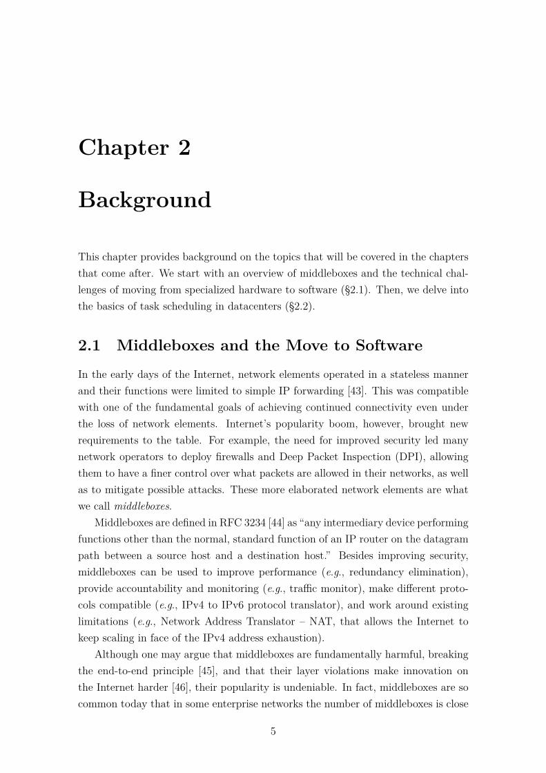
Figure 2.1: Evolution of Ethernet standards.

to the number of routers and switches [11, 12].

2.1.1 The Move to Software

Until recent years, middleboxes were primarily deployed using purpose-built hard-ware. This, however, has several shortcomings [47]:

• Rigidity: Since functionality is implemented directly on hardware, change isvery hard—often impossible.

• Hard to manage: Middleboxes from multiple vendors have their own man-agement interfaces that do not work together.

• Slow development: Hardware is slower and harder to develop than software.

• Cost: Some middleboxes are very expensive. Moreover, underutilized boxesoffer no opportunity for consolidation.

This started to change in 2012, when major carriers established a cooperationto build what they called Network Function Virtualization (NFV) [13]. NFV aimsto solve the above problems by moving middlebox functionality, called NetworkFunctions (NFs), from dedicated boxes to software running on commodity servers.The move to software, however, is not a panacea. Purpose-built hardware generallyoffers line-rate performance that is challenging to achieve in software. In fact, withthe fast adoption of higher-speed Ethernet standards, achieving line rates is onlygetting harder (see Figure 2.1).

2.1.2 Packet Processing on x86

A straightforward way of implementing NFs using software is to run an applicationon top of an operating system and leverage its network stack to receive and transmitpackets. We will now see that, although this approach works, it is not a good ideafrom a performance standpoint.

6

Kernel Space User SpaceI/O

NIC Driver Network Stack App

Interrupt Syscall

Memory

Packet BuffersCopy

Descriptor Rings / Packet BuffersDMA

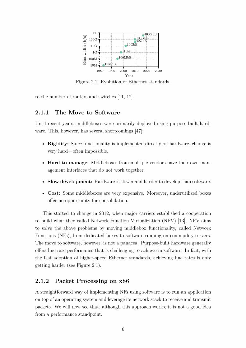
Figure 2.2: Packet processing using Linux network stack.

An application that uses the Linux network stack runs in user space and inter-acts with the stack in kernel space using system calls (syscalls). Figure 2.2 shows anoverview of packet processing using the Linux network stack, dashed arrows repre-sent control signals, while solid arrows represent data transfer. When the NetworkInterface Controller (NIC) receives a packet, it writes it to a buffer in the memory1

and issues an interrupt. The interrupt triggers the NIC driver’s interrupt handlerthat reads the packet from the buffer and passes it to the network stack. Finally,the network stack parses the packet and copies it to the application’s packet bufferin user space. A reverse process happens when the application wants to transmit apacket. The application writes the packet to memory in user space and invokes asyscall. The network stack then copies the packet to a buffer in kernel space andpasses it to the driver which informs the NIC that the packet is ready to be trans-mitted. At last, the NIC reads the packet from memory and sends it to the line,completing the transmission.

The processes above impose significant overheads, most of them due to the sep-aration between user space and kernel space. The first issue is the need to copypackets from one space to another, wasting a considerable number of CPU cycles.Another problem is the need to use syscalls and interrupts to transmit and receivepackets. Syscalls and interrupts cause a transition from user space to kernel space,which requires saving the value of some registers to memory. The reason Linuxworks like this is not because it is unconcerned with performance. Operating sys-tems are designed to make sharing hardware resources possible, the same appliesto sharing a NIC. The most common use case for an OS is not packet processing,usually different applications are running at the same time and need to receive andtransmit packets. This design makes sure that no application monopolizes the NIC,but the need for better performance in packet processing applications justifies amore restrictive design.

Since most of the overhead imposed by the Linux network stack is due to the1The ability of I/O devices to write and read directly from memory is what we call Direct

Memory Access (DMA).

7

Kernel Space User SpaceI/O

NIC UIO Driver DPDK

Syscall

Memory

Descriptor Rings / Packet BuffersDMA

App

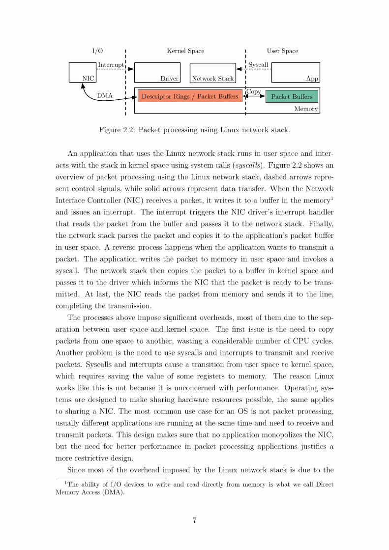
Figure 2.3: Packet processing using DPDK.

separation between user space and kernel space, a natural solution is to do packetprocessing entirely in the kernel, or entirely in user space. User-space-only packetprocessing, however, has advantages over kernel-space-only. First, kernel code mustbe low profile, running fast and yielding the CPU to user-space processes. This iscertainly not the case with high-speed packet processing, that often needs multiplededicated CPU cores (§2.1.3). Second, kernel programming is less flexible, kernelcode only has access to a limited set of libraries and is harder to debug.

There are several frameworks for high-performance packet processing in userspace, some examples include DPDK [48], netmap [49], and PF_RING ZC [50]. InChapter 3 we use DPDK for two main reasons: it has better performance [51] andit offers several libraries that aid the development of packet processing applications,e.g., lockless rings and flow classifiers. Figure 2.3 shows an overview of packetprocessing using DPDK. DPDK bypasses the kernel and communicates directly withthe NIC from user space. To do this, it replaces the NIC driver with the UIO(User-space I/O) driver, a minimal driver provided by the Linux kernel to allow thedevelopment of drivers in user space. DPDK uses the UIO driver to set up the NICand map its memory to user space. After the initialization is complete, the NICreads and writes packets directly to user-space memory and DPDK can configureNIC registers without kernel intervention. There is a problem though, since DPDKnow talks directly to the NIC it cannot use the existing kernel drivers, drivers mustbe implemented inside DPDK. This restricts the set of NICs that can work with it;only NICs that had their drivers ported to DPDK can be used.

Kernel bypass also allows DPDK to avoid the interrupt overhead. Instead ofwaiting for an interrupt, applications that use DPDK continuously check the mem-ory for new packets. This technique, known as polling, wastes CPU cycles whenthe traffic is low but achieves better performance under heavy loads. Another op-timization employed in DPDK codebase is to process batches of packets, instead ofindividual, whenever possible. These and other optimizations restrain DPDK frombeing a drop-in replacement for Linux packet socket—which is the way applicationsthat rely on Linux network stack are able to send and receive raw packets [52]. As a

8

1970 1980 1990 2000 2010 2020

Year

101

103

105

107 Transistors (thousands)

Number of logical cores

Frequency (MHz)

Single-thread performance(SpecINT ×103)

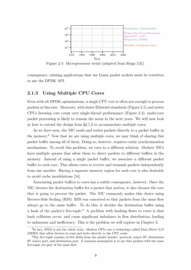
Figure 2.4: Microprocessor trend (adapted from Rupp [53]).

consequence, existing applications that use Linux packet sockets must be rewrittento use the DPDK API.

2.1.3 Using Multiple CPU Cores

Even with all DPDK optimizations, a single CPU core is often not enough to processpackets at line rate. Moreover, with faster Ethernet standards (Figure 2.1) and newerCPUs favoring core count over single-thread performance (Figure 2.4), multi-corepacket processing is likely to remain the norm in the next years. We will now lookat how to extend the design from §2.1.2 to accommodate multiple cores.

As we have seen, the NIC reads and writes packets directly to a packet buffer inthe memory.2 Now that we are using multiple cores, we may think of sharing thispacket buffer among all of them. Doing so, however, requires costly synchronizationmechanisms. To avoid this problem, we turn to a different solution. Modern NICshave multiple queues that allow them to direct packets to different buffers in thememory. Instead of using a single packet buffer, we associate a different packetbuffer to each core. This allows cores to receive and transmit packets independentlyfrom one another. Having a separate memory region for each core is also desirableto avoid cache invalidations [54].

Associating packet buffers to cores has a subtle consequence, however. Once theNIC chooses the destination buffer for a packet that arrives, it also chooses the corethat is going to process the packet. The NIC commonly makes this choice usingReceive-Side Scaling (RSS). RSS was conceived so that packets from the same flowalways go to the same buffer. To do this, it decides the destination buffer usinga hash of the packet’s five-tuple.3 A problem with hashing flows to cores is thathash collisions occur, and cause significant imbalance in flow distribution, leadingto unfairness and inefficiency. This is the problem we will explore in Chapter 3.

2In fact, DMA is not the whole story. Modern CPUs use a technology called Data Direct I/O(DDIO) that allow devices to read and write directly to the CPU cache.

3The five-tuple consists of five fields from the packet header: protocol, source IP, destinationIP, source port, and destination port. A common assumption is to say that packets with the samefive-tuple are part of the same flow.

9

Equal shareMMF allocation

User: A B C D

Figure 2.5: Resource allocation among four users using Max-Min Fairness.

2.2 Datacenter Task SchedulingClusters of commodity servers have become commonplace. They are responsible formany web services as well as a growing number of data-processing and scientificapplications. Yet, managing these clusters is no easy task [55]; cluster managersmust ensure good availability in the presence of a high number of failures [56]. Tomake matters more complicated, clusters are often shared among many users withdifferent requirements and workload types [6, 35]. Examples of cluster managersinclude open source projects such as Mesos [6] and YARN [34], as well as privatesolutions, such as Google’s Borg [57].

To use a cluster, users submit jobs composed of one or more tasks. Then, thecluster manager is responsible for scheduling these tasks. Workloads differ substan-tially among users, for example, users that run simulations and machine learningtrainings can use the cluster for hours or even days, while some that make interactiveSQL queries only need it for a few minutes [6, 35]. In a broad sense, when mul-tiple users share a system, there must be a scheduler that determines the amountof resources each user gets. The requisites for this decision vary among differentscenarios. For example, in a public cloud, users pay for the resources they use andfairness is not a concern. In contrast, in a cluster within an institution (researchcenter, lab, or company), usually users do not need to pay for the resources theyuse. This changes incentives considerably, users want to finish their jobs as fast aspossible and, when they need, will try to use the maximum amount of resources [2].

2.2.1 Resource Allocation

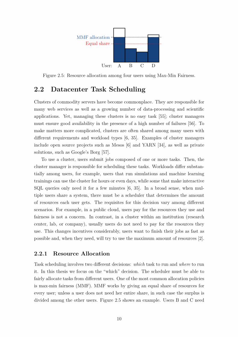
Task scheduling involves two different decisions: which task to run and where to runit. In this thesis we focus on the “which” decision. The scheduler must be able tofairly allocate tasks from different users. One of the most common allocation policiesis max-min fairness (MMF). MMF works by giving an equal share of resources forevery user; unless a user does not need her entire share, in such case the surplus isdivided among the other users. Figure 2.5 shows an example. Users B and C need

10

Memory(total: 180 GB)

CPU(total: 9)

A

A

B

B

Dominant share

Users’ Demands:User A: 4 cores 160 GBUser B: 9 cores 30 GB

DRF Allocation:User A: 3 cores 120 GBUser B: 6 cores 20 GB

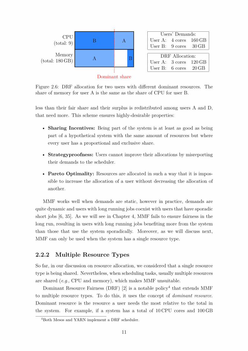
Figure 2.6: DRF allocation for two users with different dominant resources. Theshare of memory for user A is the same as the share of CPU for user B.

less than their fair share and their surplus is redistributed among users A and D,that need more. This scheme ensures highly-desirable properties:

• Sharing Incentives: Being part of the system is at least as good as beingpart of a hypothetical system with the same amount of resources but whereevery user has a proportional and exclusive share.

• Strategyproofness: Users cannot improve their allocations by misreportingtheir demands to the scheduler.

• Pareto Optimality: Resources are allocated in such a way that it is impos-sible to increase the allocation of a user without decreasing the allocation ofanother.

MMF works well when demands are static, however in practice, demands arequite dynamic and users with long running jobs coexist with users that have sporadicshort jobs [6, 35]. As we will see in Chapter 4, MMF fails to ensure fairness in thelong run, resulting in users with long running jobs benefiting more from the systemthan those that use the system sporadically. Moreover, as we will discuss next,MMF can only be used when the system has a single resource type.

2.2.2 Multiple Resource Types

So far, in our discussion on resource allocation, we considered that a single resourcetype is being shared. Nevertheless, when scheduling tasks, usually multiple resourcesare shared (e.g., CPU and memory), which makes MMF unsuitable.

Dominant Resource Fairness (DRF) [2] is a notable policy4 that extends MMFto multiple resource types. To do this, it uses the concept of dominant resource.Dominant resource is the resource a user needs the most relative to the total inthe system. For example, if a system has a total of 10 CPU cores and 100 GB

4Both Mesos and YARN implement a DRF scheduler.

11

of memory, the dominant resource for a user that needs 5 CPU cores (50%) and20 GB of memory (20%) is CPU. When allocating resources, DRF tries to equalizeusers’ share of dominant resource (dominant shares). Figure 2.6 shows an exampleof DRF allocation when two users share a system with two types of resources.User A’s dominant resource is memory, while user B’s is CPU. DRF gives each userthe same dominant share. More broadly, the DRF allocation can be obtained byapplying MMF to users’ dominant shares. This means that if a user needs less thanher dominant share, DRF will reallocate the surplus among the other users. Animportant aspect of DRF is that it inherits the MMF properties listed in §2.2.1.Moreover, when there is a single resource type, DRF reduces to MMF. By beingan extension to MMF, DRF also has problems to ensure fairness in the long run.In Chapter 4 we introduce an allocation policy that addresses these problems whileensuring the same properties.

12

Chapter 3

Sprayer

In this chapter we present Sprayer, a framework for developing network functionsusing packet spraying. Packet spraying solves the imbalance problems caused byRSS, but makes flow state handling more challenging. Sprayer uses features of com-modity NICs to spray packets to cores without software intervention. Moreover,it equips NFs with abstractions for handling flow states. Sprayer’s flow state ab-stractions build on the observation that most NFs only update flow state when TCPconnections start or finish (§3.2.2). Therefore, by directing packets at the beginningor end of the same TCP connection (connection packets) to the same core, we ensurethat only this core will need to modify the state for this connection. This avoidsthe introduction of synchronization primitives that would impact performance.

We conduct experiments to understand how effective Sprayer is in comparisonto RSS. Similarly to the datacenter observations, we find that the low differencein delay between packets processed in different cores is not enough to significantlyimpair TCP performance. Moreover, we observe that the overall TCP throughputremains consistent for both low and high number of concurrent flows. Therefore,for the typical number of concurrent flows found in real workloads, Sprayer greatlyimproves TCP throughput, compared to RSS. Further, we show that Sprayer alsoimproves fairness, even with a higher number of flows.

This chapter is organized as follows. In §3.1 we use real packet traces to motivatethe need for packet spraying in middleboxes. Then, we detail Sprayer’s design in§3.2, and implementation in §3.3. We conduct experiments to evaluate Sprayer in§3.4 and discuss its limitations in §3.5. Finally, we survey related work in §3.6 andconclude the chapter in §3.7.

3.1 MotivationTo motivate the need for packet spraying in middleboxes, we begin with a quickanalysis of real packet traces. We want to understand how diverse is the traffic at

13

103 105 107 109

Flow size (bytes)

0

0.25

0.5

0.75

1.0

CD

F

FlowsBytes

Figure 3.1: Distribution of number of flows with a given size and distribution ofbytes across different flow sizes.

0 5 10 15Concurrent flows

0.0

0.25

0.5

0.75

1.0

CD

F

All flows> 10MB

Figure 3.2: Number of concurrent flows in every 150 µs window, considering all flowsor only large flows.

the small time frame that packets stay inside a middlebox.We use a 48 h trace of a highly-utilized 1 Gbps backbone link [58] captured in

May 2018. The trace does not contain packet payloads, we determine packet sizesusing the “Total Length” field of the IP header. Figure 3.1 shows the CDF of TCPflow sizes as well as the distribution of bytes across these flows. There are few largeflows, but they are responsible for the majority of the traffic. Flows with more than10 MB account for more than 75% of the traffic. This confirms the long observed“elephants and mice” phenomenon of Internet traffic [59].

The effectiveness of RSS on middleboxes depends on the number of concurrentflows. If this number is large enough, RSS uses all cores with high probability.Although the number of ongoing TCP connections can be very large,1 if we consideronly the number of flows active in the small amount of time it takes for a packet tobe processed by a middlebox, this assumption no longer holds.

To measure concurrent flows, we use a 150 µs window. This window is 10 timesthe largest 99th percentile RTT we found in our experiments (§3.4).2 This RTT isalso comparable to the one measured by previous work [19, 47, 60]. Since the actualtime a packet takes to be processed by the middlebox is certainly less than the RTT,

1The number of ongoing TCP connections can exceed 1 million in this trace.2This RTT is measured using a server directly connected to the middlebox. We explain this

experiment in §3.4.

14

core 0

core 1

core 2

core nRSS

/ Fl

ow D

irect

orNIC(Rx)

NIC(Tx)

Figure 3.3: Hardware packet classification. The NIC is responsible for directingpackets to cores.

the number of concurrent flows we report is a strict upper bound.Figure 3.2 presents the CDF of the number of concurrent TCP flows. The

median number of concurrent flows is only 4 and the 99th percentile is 14. Thelevel of concurrency among large flows is even smaller. If we only consider flowswith more than 10 MB, the median number of concurrent flows is 1 and the 99th

percentile is 6. Yet, as we have seen, these flows account for the majority of thetraffic, which indicates a poor degree of statistical multiplexing.

Since these results are for a backbone link, we expect them to include more con-current flows than the traffic of an enterprise network. Indeed, we repeated the sameanalysis on traffic at our lab’s Internet gateway and on the M57 traces [61] (usedby some previous work on middleboxes [18, 23]) and found even fewer concurrentflows.

3.2 DesignWe now turn to the design of Sprayer. First we describe the challenges of processingsprayed packets. Then we present an architecture that deals with these challenges.Finally, we delve into a simple programming model used by NFs implemented ontop of Sprayer.

There are two main challenges in the design of Sprayer: spraying packets todifferent cores and handling flow states.

3.2.1 How to spray packets?

When processing packets in a multi-core system, one has to choose between softwareand hardware packet classification. As depicted in Figure 3.3, the hardware tech-nique consists of using multi-queue NICs, which are common today, to classify anddirect packets to each core. The software alternative is to direct all packets to a sin-

15

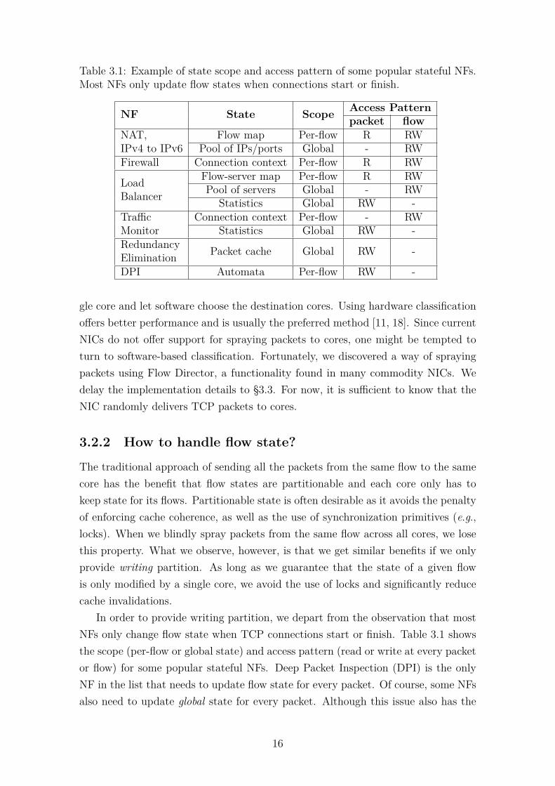
Table 3.1: Example of state scope and access pattern of some popular stateful NFs.Most NFs only update flow states when connections start or finish.

NF State Scope Access Patternpacket flow

NAT,IPv4 to IPv6

Flow map Per-flow R RWPool of IPs/ports Global - RW

Firewall Connection context Per-flow R RW

LoadBalancer

Flow-server map Per-flow R RWPool of servers Global - RW

Statistics Global RW -TrafficMonitor

Connection context Per-flow - RWStatistics Global RW -

RedundancyElimination Packet cache Global RW -

DPI Automata Per-flow RW -

gle core and let software choose the destination cores. Using hardware classificationoffers better performance and is usually the preferred method [11, 18]. Since currentNICs do not offer support for spraying packets to cores, one might be tempted toturn to software-based classification. Fortunately, we discovered a way of sprayingpackets using Flow Director, a functionality found in many commodity NICs. Wedelay the implementation details to §3.3. For now, it is sufficient to know that theNIC randomly delivers TCP packets to cores.

3.2.2 How to handle flow state?

The traditional approach of sending all the packets from the same flow to the samecore has the benefit that flow states are partitionable and each core only has tokeep state for its flows. Partitionable state is often desirable as it avoids the penaltyof enforcing cache coherence, as well as the use of synchronization primitives (e.g.,locks). When we blindly spray packets from the same flow across all cores, we losethis property. What we observe, however, is that we get similar benefits if we onlyprovide writing partition. As long as we guarantee that the state of a given flowis only modified by a single core, we avoid the use of locks and significantly reducecache invalidations.

In order to provide writing partition, we depart from the observation that mostNFs only change flow state when TCP connections start or finish. Table 3.1 showsthe scope (per-flow or global state) and access pattern (read or write at every packetor flow) for some popular stateful NFs. Deep Packet Inspection (DPI) is the onlyNF in the list that needs to update flow state for every packet. Of course, some NFsalso need to update global state for every packet. Although this issue also has the

16

NIC

NFregular_packets

Flow Table

SYN/FIN/RST ?

NFconnection_packets

Core Other Cores

Core picker

Flow Table

RRW

NFNFRW

DataState

Y N

foreignlocal

foreignpackets

ringring

Figure 3.4: Overview of Sprayer from the perspective of a single core. Regularpackets are processed locally, while connection packets may be transferred to othercores.

potential to affect performance, it is not specific to Sprayer, traditional approachesmust also deal with shared global state. Moreover—at least in the case of statistics—looser consistency is often tolerable, which helps to reduce the problem [25].

We make a distinction between connection packets and regular packets. Con-nection packets are those that have potential to modify TCP state (packets flaggedwith SYN, FIN, or RST), while regular packets are all the others. Moreover, we saythat every flow has a designated core. We determine the designated core for a givenflow calculating a hash of its five-tuple. By default, we use a hash function thatmaps upstream and downstream flows from the same TCP connection to the samedesignated core. Sprayer enforces writing partition by keeping flow states in theirdesignated cores while making sure that all connection packets from a given floware processed in their designated core.

3.2.3 Architecture

Figure 3.4 shows an overview of Sprayer’s architecture. The key idea is to separatethe NF code that handles connection packets from the code that handles regularones. All cores run identical threads and have their own flow tables. Moreover,cores can only write to their local flow tables, but can read from any. This ensureswriting partition.

After the NIC delivers a packet, Sprayer checks whether it is a connection packet.

17

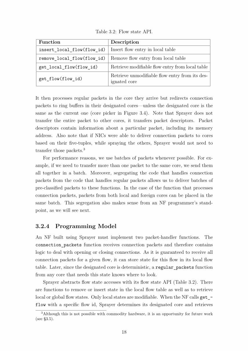
Table 3.2: Flow state API.

Function Descriptioninsert_local_flow(flow_id) Insert flow entry in local tableremove_local_flow(flow_id) Remove flow entry from local tableget_local_flow(flow_id) Retrieve modifiable flow entry from local table

get_flow(flow_id) Retrieve unmodifiable flow entry from its des-ignated core

It then processes regular packets in the core they arrive but redirects connectionpackets to ring buffers in their designated cores—unless the designated core is thesame as the current one (core picker in Figure 3.4). Note that Sprayer does nottransfer the entire packet to other cores, it transfers packet descriptors. Packetdescriptors contain information about a particular packet, including its memoryaddress. Also note that if NICs were able to deliver connection packets to coresbased on their five-tuples, while spraying the others, Sprayer would not need totransfer those packets.3

For performance reasons, we use batches of packets whenever possible. For ex-ample, if we need to transfer more than one packet to the same core, we send themall together in a batch. Moreover, segregating the code that handles connectionpackets from the code that handles regular packets allows us to deliver batches ofpre-classified packets to these functions. In the case of the function that processesconnection packets, packets from both local and foreign cores can be placed in thesame batch. This segregation also makes sense from an NF programmer’s stand-point, as we will see next.

3.2.4 Programming Model

An NF built using Sprayer must implement two packet-handler functions. Theconnection_packets function receives connection packets and therefore containslogic to deal with opening or closing connections. As it is guaranteed to receive allconnection packets for a given flow, it can store state for this flow in its local flowtable. Later, since the designated core is deterministic, a regular_packets functionfrom any core that needs this state knows where to look.

Sprayer abstracts flow state accesses with its flow state API (Table 3.2). Thereare functions to remove or insert state in the local flow table as well as to retrievelocal or global flow states. Only local states are modifiable. When the NF calls get_-flow with a specific flow id, Sprayer determines its designated core and retrieves

3Although this is not possible with commodity hardware, it is an opportunity for future work(see §3.5).

18

the flow state from its flow table. Note that the constness of the flow entry returnedby the get_flow function is only lightly enforced, we use a C pointer to a constvariable, that means that a programmer may remove the constness and modifythe variable. Although removing this constness is possible, it may cause undefinedbehavior, and on some situations triggers compiler warnings. Besides the functionsin Table 3.2, Sprayer has an optimized version of get_flow for looking up multipleflow states at a time.

Of course, there is much more complexity in programming an NF than flowstate access. Our focus here is not in providing a comprehensive set of tools forNF programming—others have done it already [47, 62, 63]—instead we argue thatSprayer’s flow state abstractions are simple to use and can be incorporated to othersolutions.

We use a simple implementation of a NAT to demonstrate how to use Sprayer’sflow state abstractions (Figure 3.5). For brevity, we only consider TCP packets, andomit variable declarations and flow removal logic. Moreover, a real implementationwill use batches of packets instead of separately handling each. The connection_-packets function, upon receiving the first SYN packet from a TCP connection, selectsa port from a global pool (line 10) and uses insert_local_flow to save this trans-lation in the local flow table (lines 18–19). Since the designated core is the samefor both sides of the same TCP connection, the NAT can also store the translationfor the other side (lines 25–26). NAT then treats all the packets that come after(including SYN-ACK) as regular packets. The regular_packets function only hasto retrieve the translation using get_flow (line 31) and use it to update the packetheader (line 39). Sprayer API also helps NFs that need to record statistics buttolerate looser consistency. These NFs can keep statistics for all flows in every coreand periodically aggregate them in their designated cores.

In addition to packet handlers, Sprayer also allows NFs to implement an initial-ization function. Besides initialization work (e.g., memory allocation), NFs can usethis function to set parameters that Sprayer will use in its own initialization, such asthe size of the flow table and its entries. Stateless NFs can also set a flag to disableflow state features, i.e., flow tables and the redirection of connection packets.

3.3 ImplementationWe have implemented Sprayer on top of DPDK [48], taking advantage of manystate-of-the-art optimizations, such as polling and batching. In order to make theNIC spray packets we also had to modify DPDK’s ixgbe driver [64]. At first glance,it may seem impossible to spray packets using existing commodity NICs, since theydo not offer this functionality [65, 66]. We, however, circumvent this limitation using

19

1 void connection_packets(pkt_t* pkt) {2 // we only care about the first SYN packet3 if (!pkt->SYN || pkt->ACK) {4 regular_packets(pkt);5 return;6 }7 flow_id = get_five_tuple(pkt);8

9 // select a port from pool10 translated_flow_id = select_port(flow_id);11

12 // no port available or invalid source IP13 if (!translated_flow_id) {14 drop_packet(pkt);15 return;16 }17

18 flow_entry = insert_local_flow(flow_id);19 *flow_entry = translated_flow_id;20

21 update_header(pkt, translated_flow_id);22

23 // we also include the other side24 rev_flow_id = reverse(translated_flow_id);25 flow_entry = insert_local_flow(rev_flow_id);26 *flow_entry = reverse(flow_id);27 }28

29 void regular_packets(pkt_t* pkt) {30 flow_id = get_five_tuple(pkt);31 translated_flow_id = get_flow(flow_id);32

33 // no translation found for this flow id34 if (!translated_flow_id) {35 drop_packet(pkt);36 return;37 }38

39 update_header(pkt, translated_flow_id);40 }

Figure 3.5: Sample implementation of a NAT. Sprayer’s API functions and packethandlers are underlined.

20

Flow Director [65], a feature of Intel NICs designed to associate specific sets of flowsto queues. We use Flow Director in an unconventional manner: instead of matchingflows, we configure it such that packets are directed to queues using the checksumfield of the TCP header. Since the checksum field looks random, TCP packets areuniformly distributed across queues regardless of their flows. In contrast, non-TCPpackets fail to match any rules and fall back to traditional RSS, in which the NICdirects packets to cores using a hash of the five-tuple. All non-TCP packets areprocessed in the core they arrive, with no need for redirection.

A major problem with Flow Director—and in fact the reason many choose not touse it [15, 60]—is that it has a somewhat limited space for flow rules (8k). We avoidthis problem using only a certain number of least significant bits of the checksumfield, depending on the number of cores in the system. This allow us to define rulesthat exhaust all possible matches.

3.4 EvaluationThis section presents an evaluation of Sprayer. We run experiments on a testbedwith two servers connected back-to-back. One server functions as a traffic generatorand the other as a middlebox. The middlebox server is equipped with two IntelXeon E5-2650 CPUs, each of which has 8 cores with 2.0 GHz clock, and 256 GB ofRAM (equally divided among all memory channels). The traffic-generator serveris equipped with a single Intel Core i7-7700 CPU and 32 GB of RAM. Moreover,both servers have an Intel 82599ES 10 GbE NIC [65] and run Linux 4.9.0-5. Weconfigure the RSS hash function to direct upstream and downstream flows from thesame connection to the same core [67].

To systematically emulate NFs with different complexities, we implement a sim-ple NF on top of Sprayer. This NF creates a new entry in the flow table at everynew connection. Moreover, for every packet it receives, it retrieves the flow state,modifies the header, and busy loops for a given number of cycles. We vary thenumber of cycles from 0 up to 10,000 (the maximum number of cycles per packetamong the NFs surveyed by [20]). The NF uses 8 cores in all experiments.

When measuring processing rate, we use MoonGen [68] to generate 64 B TCPpackets with variable payload content, and therefore variable checksum. Whenmeasuring TCP throughput, we use Iperf3 [69] to create real TCP connections. Ourresults use the standard Linux TCP implementation (CUBIC), without any kind oftuning. Unless otherwise noted, error bars represent one standard deviation.

How much can Sprayer improve performance? The maximum improvementcaused by Sprayer happens when there is a single flow. Figure 3.6a shows the

21

0 2000 4000 6000 8000 10000

Processing cycles per packet

0.0

2.5

5.0

7.5

10.0Pr

oces

sing

rate

(Mpp

s)RSSSprayer

(a) Processing rate.

0 2000 4000 6000 8000 10000


2

4

6

8

10

Thr

ough

put

(Gbp

s)

RSSSprayer

(b) TCP throughput.

Figure 3.6: Effect of increasing the number of processing cycles per packet on pro-cessing rate (with 64 B packets) and TCP throughput, while using a single flow.

100 101 102

Number of flows

0.5

1.0

1.5

Proc

essin

gra

te(M

pps)

RSSSprayer

(a) Processing rate.

100 101 102

Number of flows

2

4

6

8

10

Thr

ough

put

(Gbp

s)

RSSSprayer

(b) TCP throughput.

Figure 3.7: Effect of increasing the number of flows on processing rate (with 64 Bpackets) and TCP throughput. Processing cycles per packet remain fixed at 10,000.

processing rate as a function of per-packet processing cycles for a single flow. Asexpected, when we increase the number of cycles spent on each packet, the processingrate decreases. Somewhat unexpectedly though, Sprayer’s processing rate is limitedto about 10 Mpps. This, however, is not fundamental and is a limitation of the82599 NIC when using Flow Director. For less trivial NFs, the fact that Sprayeruses all cores allows it to process significantly more packets than RSS. Since Sprayermay reorder packets, improving processing rate does not necessarily improve TCPthroughput. Figure 3.6b alleviates this concern by measuring the throughput of areal TCP connection.

How does the number of flows impact Sprayer? The performance of Sprayeris consistent regardless of the number of concurrent flows. We repeat the sameexperiments fixing the number of processing cycles per packet in 10,000 while in-creasing the number of flows. Sources and destinations change randomly at everyexecution. When generating packets from different flows using MoonGen, we useround-robin, so that packets from different flows are perfectly interleaved—this isthe best-case scenario for RSS. Figure 3.7 compares the processing rate and TCP

22

0 2000 4000 6000 8000 10000


10

15

20

Late

ncy

(µs)

RSSSprayer

Figure 3.8: 99th percentile RTT for 64 B packets at 70% load for a single flow.

100 101 102

Number of flows

0.7

0.8

0.9

1.0

Jain

’sfa

irnes

sin

dex

RSSSprayer

Figure 3.9: Jain’s fairness index for an increasing number of flows.

throughput of RSS and Sprayer, for increasing numbers of concurrent flows. Wefind that RSS shows considerably worse throughput for a small number of flowsand a slightly better throughput for a sufficiently large number of flows. Since theprocessing rate between the two is similar for a large number of flows, we attributethe difference in TCP throughput to packet reordering. Furthermore, if we considerthe small number of concurrent flows in a typical workload (Figure 3.2), Sprayeris faster most of the time. Also note, that the measurements for RSS have largererror bars. That is because hash collisions change from one experiment to another,causing better or worse throughput.

Does Sprayer impact latency? Since Sprayer spreads packets from the sameflow across all cores, packets from the same flow are processed in parallel. This endsup reducing latency. Figure 3.8 compares the 99th percentile round trip time whenusing RSS and Sprayer to process 64 B packets from a single flow at 70% of theminimal processing rate between RSS and Sprayer.

Does Sprayer impact fairness? Sprayer eliminates the fairness problem causedby hash collisions. Since all flows get to share all cores equally, they all receive thesame share. Figure 3.9 reports the average Jain’s fairness index [7] across all runs.Error bars represent the minimum and maximum observations. While Sprayer con-sistently achieves fair throughput (Jain’s index close to 1.0), RSS’s fairness dependson the number of flows each core has to process.

23

Summary. Our experiments indicate that spraying packets across cores is a validapproach for software middleboxes. It improves fairness and provides consistentperformance, regardless of the number of flows. What remains to be answered ishow well other TCP implementations interact with the levels of packet reorderingimposed by Sprayer. Moreover, although the NF used in our experiments operatessimilarly to a real NF,4 we plan to extend our evaluation to real NFs implementedon top of Sprayer.

3.5 DiscussionWe now point to Sprayer’s limitations and outline questions that should be furtherinvestigated.

NF deployability: Sprayer’s programming model can be used to implement NFsthat do not need to update flow state in the middle of a flow (e.g., NAT, firewall,load balancer, traffic monitor). However, not every NF fits this model. Some DPIs,for example, need to support cross-packet pattern matching. Although they can bemade to work with out-of-order packets [70], implementing them on top of Sprayerwould require that cores share their state machines. Another example of NFs in-compatible with Sprayer are transparent web proxies and caches. The reason beingthat an HTTP request may be split among different TCP packets and end up goingto different cores. Since transparent proxies are incompatible with HTTPS—whichnow accounts for more than 70% of loaded web pages [71, 72]—we do not see thisas a major drawback.

Programmable NICs: We constrained our design to work on commodity hard-ware. However, the rise of programmable NICs [73–75] creates further opportunities.First, we could program NICs to direct connection packets to designated cores, re-ducing some of Sprayer’s overhead. Also, inspired by previous work on datacenternetworks [76–78], we may configure NICs to direct packets to cores using flowlets.Flowlets are a middle ground between packets and flows. They are based on theobservation that packets from the same flow often arrive in bursts. Datacentersthat use flowlets direct these bursts of packets to the same path. This can bringadvantages, such as reduced packet reordering.

Scalability with more cores: Although an increase in the number of CPU coresshould increase Sprayer’s advantage over RSS, it also has the potential to increasepacket reordering. Therefore, it may be wise to only spray packets from a particular

4Our NF does a flow-state lookup, updates the header, and busy-loops for a certain number ofcycles. A firewall, for example, would lookup the flow state and go through an access control list(ACL).

24

flow to a limited subset of cores [79]. We intend to test this hypothesis in futurework using programmable NICs.

Elastic scaling to multiple hosts: In this work we focused on improving utiliza-tion of a single host. In some situations, however, NFs need to scale to multiplehosts [17, 23–25]. We can also scale Sprayer to multiple hosts, as long as packetsfrom the same flow are not sprayed across different hosts. Moreover, proposals likeS6 [25], that advocates using a Distributed Shared Object (DSO) to share stateamong hosts, could also be used to scale Sprayer.

Different transport protocols: At our current implementation, Sprayer onlysprays TCP packets; other packets continue to be directed to cores using RSS. Thisavoids the potential problems packet reordering causes to some UDP applications(e.g., VoIP [78]). More elaborated classification could be made to spray only someUDP flows. QUIC [46], for example, runs on top of UDP and by design is moreresilient to packet reordering than TCP.

3.6 Related WorkAs already mentioned, there are multiple works that use packet spraying to improveboth efficiency and fairness in datacenter networks [10, 29–32]. Yet, Sprayer isthe first to bring this concept to software middleboxes. Although the basic idea issimilar, the implications are different. One of the challenges of using packet sprayingin datacenters is to ensure that it keeps working in the presence of asymmetriescaused by link failures. In middleboxes, this problem does not exist. Instead, flowstate sharing is the main concern.

Many previous works have also investigated NF state so as to scale NFs tomultiple hosts [17, 22–25]. Despite these solutions being orthogonal to our work, theyhave identified similar flow-state-access patterns as we did. Moreover, one of thesesolutions, StatelessNF [23], moves all NF state (per-flow and global) to a remoteserver, which is an elegant approach to simplifying scalability and failure recovery.Although StatelessNF could potentially replace Sprayer’s flow state abstractions, itrequires non-commodity technology (InfiniBand). Moreover, accessing remote statesincreases latency and requires extra CPU cycles [25].

Some attempts have also been made to improve middlebox efficiency when pack-ets need to go through multiple NFs (NF chaining). Solutions such as NFP [19]and ParaBox [80] explore parallelism by processing the same packet in NFs locatedin different cores at the same time. These solutions, however, are specific to NFchaining and can only work for some configurations. Moreover, they require at leasttwo inter-core transfers for every packet. Also related to NF chaining, NFVnice [16]

25

tries to improve fairness among NFs running on the same core, but makes no effortto improve fairness among flows.

Finally, mOS [62] has focused on creating abstractions for stateful flow process-ing. It keeps track of TCP state machines and let NFs implement handlers, whichare triggered in the presence of events (e.g., new TCP connection). This is comple-mentary to Sprayer’s flow state abstractions, that facilitate flow state access in thepresence of packet spraying.

3.7 ConclusionIn this chapter, we introduced Sprayer. Sprayer allows NFs to load balance packetsto multiple CPU cores using packet spraying, instead of flow-based hashing. It alsoprovides abstractions for handling flow state without the need for synchronizationprimitives. We observed that, when compared to the per-flow alternative, Sprayersignificantly improves fairness and consistently uses the entire capacity, even whenthere is a single flow.

26

Chapter 4

Stateful Dominant ResourceFairness

In this chapter we introduce Stateful Dominant Resource Fairness (SDRF), an ex-tension of DRF that accounts for the past behavior of users and improves fairness inthe long run. The key idea is to make users with lower average usage have priorityover users with higher average usage. When scheduling tasks, SDRF ensures thatusers that only sporadically use the system have their tasks scheduled faster thanusers with continuous high usage. The intuition for SDRF is that when users usemore resources than their rightful share of the system, they commit to use less inthe future if another user needs. SDRF tracks users commitments and ensures thatwhenever system resources are insufficient, commitments are honored.

We conduct a thorough evaluation of SDRF and show that it satisfies the fun-damental properties of DRF. SDRF is strategyproof as users cannot improve theirallocation by lying to the mechanism. SDRF provides sharing incentives as no useris better off if resources are equally partitioned. Moreover, SDRF is Pareto effi-cient as no user can have her allocation improved without decreasing another user’sallocation. DRF can be efficiently implemented using a priority queue that deter-mines which user has the highest allocation priority. When we consider the past,allocation priorities may change at any instant and the implementation cannot ben-efit from a priority queue. We mitigate this problem—being able to implementSDRF efficiently—introducing live tree, a data structure that keeps elements withpredictable time-varying priorities sorted.

Besides the theoretical evaluation, we analyze SDRF using large-scale simula-tions based on Google cluster traces containing 30 million tasks over a one-monthperiod, and compare it to regular DRF. Results show that SDRF reduces the av-erage time users wait for their tasks to be scheduled. Moreover, it increases thenumber of completed tasks for users with lower demands, with negligible impact onhigh-demand users. We also use Google cluster traces to evaluate the performance

27

of live tree, concluding that SDRF works well in practice.This chapter is organized as follows. We introduce the system model in §4.1 and

use it to define DRF and its allocation properties in §4.2. We then introduce SDRFand show its properties in §4.3. In §4.4 we focus on the implementation of SDRFusing a live tree. We then test SDRF and our implementation under trace-drivensimulations in §4.5. Finally, we review related work in §4.6 and conclude the chapterin §4.7.

4.1 System ModelIn this section, we model the multi-resource allocation problem in a multi-user sys-tem. We first formalize users and resource demands, and then define the generalstructure of an allocation mechanism. From this structure we formalize users’ se-quential interactions as a repeated game.

4.1.1 Multi-Resource Setting and Allocation Mechanism

The system consists of a set of users N = {1, . . . , n} that share a pool of differenthardware resources R = {1, . . . ,m}. Without loss of generality, we normalize thetotal amount of every resource in the system to 1, i.e., if a system has a total of 100CPU cores and 10 TB of memory, 0.1 CPU equals 10 cores while 0.1 memory equals1 TB. For simplicity, we assume that the set of users and the amount of resourcesremain fixed. Every user i has a demands vector θ

(t)i = ⟨θ(t)i1 , . . . , θ

(t)im⟩ representing

the user demand for every resource at instant t. We consider positive demands forevery resource type,1 therefore at every instant t, θ(t)ir > 0,∀i ∈ N , r ∈ R.

The allocation mechanism should produce as output a resource allocation basedon users’ declared demands. We represent the declared demands vector for a user i

at instant t analogously to the demands vector, θ(t)i = ⟨θ(t)i1 , . . . , θ

(t)im⟩. When users

declare demands truthfully, θ(t)i = θ

(t)i . We also define the allocation vector for

user i at instant t for every resource type as o(t)i = ⟨o(t)i1 , . . . , o

(t)im⟩. The allocation re-

turned by the mechanism at instant t is represented by a matrix of all the individualallocation vectors: O(t) = ⟨o(t)

1 , . . . ,o(t)n ⟩. We impose a feasibility restriction to the

allocations so that they may never be greater than the total amount of resources inthe system, i.e., at every instant t,

∑i∈N o

(t)ir ≤ 1, ∀r ∈ R.

We represent user’s preferences using a utility function. Given an arbitrary1The requirement of non-zero demands is to avoid problems in the model. In practice, users

may not need every resource type at every instant. We can still use the same model and say thatthese users need ϵ resources, where ϵ is an arbitrarily small positive quantity.

28

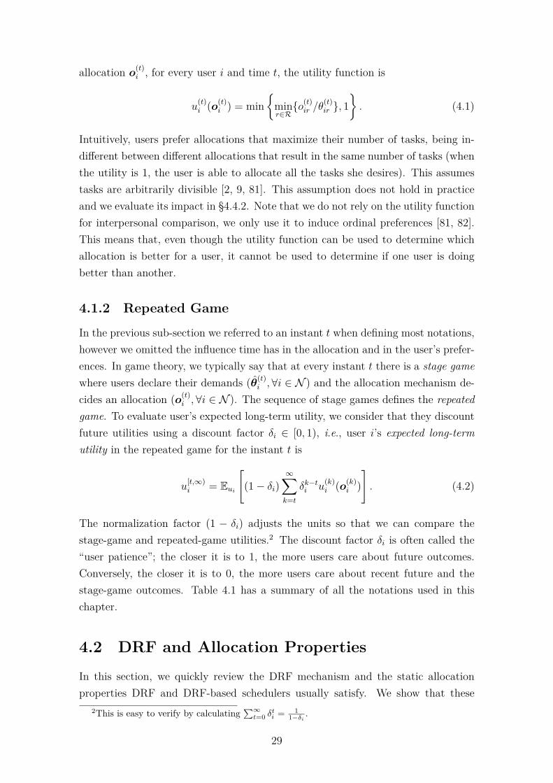
allocation o(t)i , for every user i and time t, the utility function is

u(t)i (o

(t)i ) = min

{minr∈R{o(t)ir /θ

(t)ir }, 1

}. (4.1)

Intuitively, users prefer allocations that maximize their number of tasks, being in-different between different allocations that result in the same number of tasks (whenthe utility is 1, the user is able to allocate all the tasks she desires). This assumestasks are arbitrarily divisible [2, 9, 81]. This assumption does not hold in practiceand we evaluate its impact in §4.4.2. Note that we do not rely on the utility functionfor interpersonal comparison, we only use it to induce ordinal preferences [81, 82].This means that, even though the utility function can be used to determine whichallocation is better for a user, it cannot be used to determine if one user is doingbetter than another.

4.1.2 Repeated Game

In the previous sub-section we referred to an instant t when defining most notations,however we omitted the influence time has in the allocation and in the user’s prefer-ences. In game theory, we typically say that at every instant t there is a stage gamewhere users declare their demands (θ(t)

i ,∀i ∈ N ) and the allocation mechanism de-cides an allocation (o(t)

i ,∀i ∈ N ). The sequence of stage games defines the repeatedgame. To evaluate user’s expected long-term utility, we consider that they discountfuture utilities using a discount factor δi ∈ [0, 1), i.e., user i’s expected long-termutility in the repeated game for the instant t is

u[t,∞)i = Eui

[(1− δi)

∞∑k=t

δk−ti u

(k)i (o

(k)i )

]. (4.2)

The normalization factor (1 − δi) adjusts the units so that we can compare thestage-game and repeated-game utilities.2 The discount factor δi is often called the“user patience”; the closer it is to 1, the more users care about future outcomes.Conversely, the closer it is to 0, the more users care about recent future and thestage-game outcomes. Table 4.1 has a summary of all the notations used in thischapter.

4.2 DRF and Allocation PropertiesIn this section, we quickly review the DRF mechanism and the static allocationproperties DRF and DRF-based schedulers usually satisfy. We show that these

2This is easy to verify by calculating∑∞

t=0 δti =

11−δi

.

29

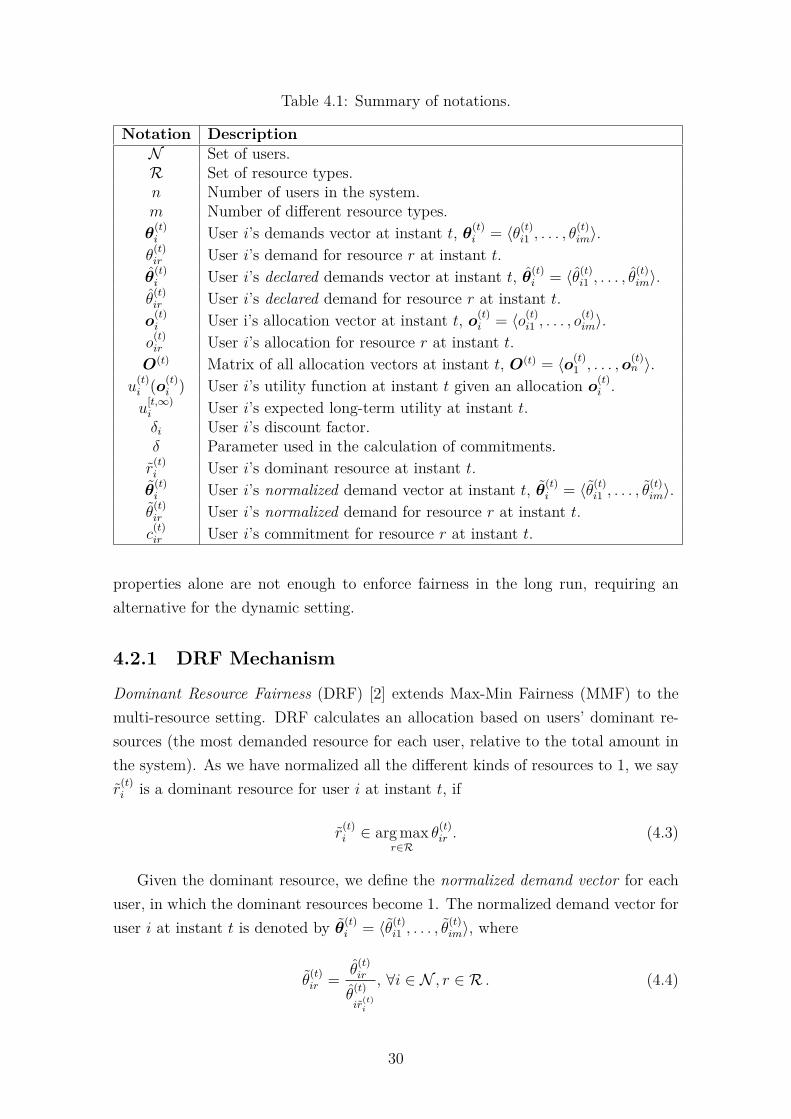
Table 4.1: Summary of notations.

Notation DescriptionN Set of users.R Set of resource types.n Number of users in the system.m Number of different resource types.θ(t)i User i’s demands vector at instant t, θ(t)

i = ⟨θ(t)i1 , . . . , θ(t)im⟩.

θ(t)ir User i’s demand for resource r at instant t.

θ(t)i User i’s declared demands vector at instant t, θ(t)

i = ⟨θ(t)i1 , . . . , θ(t)im⟩.

θ(t)ir User i’s declared demand for resource r at instant t.

o(t)i User i’s allocation vector at instant t, o(t)

i = ⟨o(t)i1 , . . . , o(t)im⟩.

o(t)ir User i’s allocation for resource r at instant t.

O(t) Matrix of all allocation vectors at instant t, O(t) = ⟨o(t)1 , . . . ,o

(t)n ⟩.

u(t)i (o

(t)i ) User i’s utility function at instant t given an allocation o

(t)i .

u[t,∞)i User i’s expected long-term utility at instant t.δi User i’s discount factor.δ Parameter used in the calculation of commitments.r(t)i User i’s dominant resource at instant t.

θ(t)i User i’s normalized demand vector at instant t, θ(t)

i = ⟨θ(t)i1 , . . . , θ(t)im⟩.

θ(t)ir User i’s normalized demand for resource r at instant t.c(t)ir User i’s commitment for resource r at instant t.

properties alone are not enough to enforce fairness in the long run, requiring analternative for the dynamic setting.

4.2.1 DRF Mechanism

Dominant Resource Fairness (DRF) [2] extends Max-Min Fairness (MMF) to themulti-resource setting. DRF calculates an allocation based on users’ dominant re-sources (the most demanded resource for each user, relative to the total amount inthe system). As we have normalized all the different kinds of resources to 1, we sayr(t)i is a dominant resource for user i at instant t, if

r(t)i ∈ arg max

r∈Rθ(t)ir . (4.3)

Given the dominant resource, we define the normalized demand vector for eachuser, in which the dominant resources become 1. The normalized demand vector foruser i at instant t is denoted by θ

(t)i = ⟨θ(t)i1 , . . . , θ

(t)im⟩, where

θ(t)ir =

θ(t)ir

θ(t)

ir(t)i

, ∀i ∈ N , r ∈ R . (4.4)

30

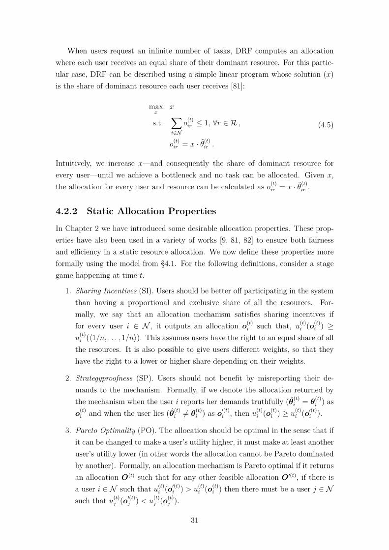
When users request an infinite number of tasks, DRF computes an allocationwhere each user receives an equal share of their dominant resource. For this partic-ular case, DRF can be described using a simple linear program whose solution (x)is the share of dominant resource each user receives [81]:

maxx

x

s.t.∑i∈N

o(t)ir ≤ 1, ∀r ∈ R ,

o(t)ir = x · θ(t)ir .

(4.5)

Intuitively, we increase x—and consequently the share of dominant resource forevery user—until we achieve a bottleneck and no task can be allocated. Given x,the allocation for every user and resource can be calculated as o

(t)ir = x · θ(t)ir .

4.2.2 Static Allocation Properties

In Chapter 2 we have introduced some desirable allocation properties. These prop-erties have also been used in a variety of works [9, 81, 82] to ensure both fairnessand efficiency in a static resource allocation. We now define these properties moreformally using the model from §4.1. For the following definitions, consider a stagegame happening at time t.

1. Sharing Incentives (SI). Users should be better off participating in the systemthan having a proportional and exclusive share of all the resources. For-mally, we say that an allocation mechanism satisfies sharing incentives iffor every user i ∈ N , it outputs an allocation o

(t)i such that, u

(t)i (o

(t)i ) ≥

u(t)i (⟨1/n, . . . , 1/n⟩). This assumes users have the right to an equal share of all

the resources. It is also possible to give users different weights, so that theyhave the right to a lower or higher share depending on their weights.

2. Strategyproofness (SP). Users should not benefit by misreporting their de-mands to the mechanism. Formally, if we denote the allocation returned bythe mechanism when the user i reports her demands truthfully (θ(t)

i = θ(t)i ) as

o(t)i and when the user lies (θ(t)

i = θ(t)i ) as o

′(t)i , then u

(t)i (o

(t)i ) ≥ u

(t)i (o

′(t)i ).

3. Pareto Optimality (PO). The allocation should be optimal in the sense that ifit can be changed to make a user’s utility higher, it must make at least anotheruser’s utility lower (in other words the allocation cannot be Pareto dominatedby another). Formally, an allocation mechanism is Pareto optimal if it returnsan allocation O(t) such that for any other feasible allocation O′(t), if there isa user i ∈ N such that u

(t)i (o

′(t)i ) > u

(t)i (o

(t)i ) then there must be a user j ∈ N

such that u(t)j (o

′(t)j ) < u

(t)j (o

(t)j ).

31

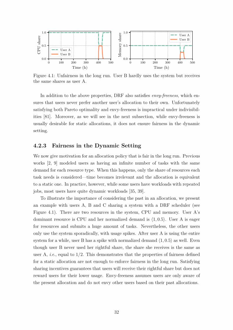
0 100 200 300 400 500

Time (h)

0.0

0.5

1.0

CPU

shar

e

User AUser B

0 100 200 300 400 500

Time (h)

0.0

0.5

1.0

Mem

ory

shar

e User AUser B

Figure 4.1: Unfairness in the long run. User B hardly uses the system but receivesthe same shares as user A.

In addition to the above properties, DRF also satisfies envy-freeness, which en-sures that users never prefer another user’s allocation to their own. Unfortunatelysatisfying both Pareto optimality and envy-freeness is impractical under indivisibil-ities [81]. Moreover, as we will see in the next subsection, while envy-freeness isusually desirable for static allocations, it does not ensure fairness in the dynamicsetting.

4.2.3 Fairness in the Dynamic Setting

We now give motivation for an allocation policy that is fair in the long run. Previousworks [2, 9] modeled users as having an infinite number of tasks with the samedemand for each resource type. When this happens, only the share of resources eachtask needs is considered—time becomes irrelevant and the allocation is equivalentto a static one. In practice, however, while some users have workloads with repeatedjobs, most users have quite dynamic workloads [35, 39].

To illustrate the importance of considering the past in an allocation, we presentan example with users A, B and C sharing a system with a DRF scheduler (seeFigure 4.1). There are two resources in the system, CPU and memory. User A’sdominant resource is CPU and her normalized demand is ⟨1, 0.5⟩. User A is eagerfor resources and submits a huge amount of tasks. Nevertheless, the other usersonly use the system sporadically, with usage spikes. After user A is using the entiresystem for a while, user B has a spike with normalized demand ⟨1, 0.5⟩ as well. Eventhough user B never used her rightful share, the share she receives is the same asuser A, i.e., equal to 1/2. This demonstrates that the properties of fairness definedfor a static allocation are not enough to enforce fairness in the long run. Satisfyingsharing incentives guarantees that users will receive their rightful share but does notreward users for their lower usage. Envy-freeness assumes users are only aware ofthe present allocation and do not envy other users based on their past allocations.

32

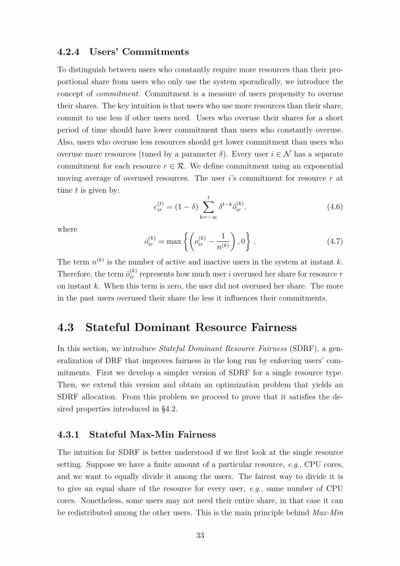
4.2.4 Users’ Commitments

To distinguish between users who constantly require more resources than their pro-portional share from users who only use the system sporadically, we introduce theconcept of commitment. Commitment is a measure of users propensity to overusetheir shares. The key intuition is that users who use more resources than their share,commit to use less if other users need. Users who overuse their shares for a shortperiod of time should have lower commitment than users who constantly overuse.Also, users who overuse less resources should get lower commitment than users whooveruse more resources (tuned by a parameter δ). Every user i ∈ N has a separatecommitment for each resource r ∈ R. We define commitment using an exponentialmoving average of overused resources. The user i’s commitment for resource r attime t is given by:

c(t)ir = (1− δ)

t∑k=−∞

δt−ko(k)ir , (4.6)

whereo(k)ir = max

{(o(k)ir −

1

n(k)

), 0

}. (4.7)

The term n(k) is the number of active and inactive users in the system at instant k.Therefore, the term o

(k)ir represents how much user i overused her share for resource r

on instant k. When this term is zero, the user did not overused her share. The morein the past users overused their share the less it influences their commitments.

4.3 Stateful Dominant Resource FairnessIn this section, we introduce Stateful Dominant Resource Fairness (SDRF), a gen-eralization of DRF that improves fairness in the long run by enforcing users’ com-mitments. First we develop a simpler version of SDRF for a single resource type.Then, we extend this version and obtain an optimization problem that yields anSDRF allocation. From this problem we proceed to prove that it satisfies the de-sired properties introduced in §4.2.

4.3.1 Stateful Max-Min Fairness

The intuition for SDRF is better understood if we first look at the single resourcesetting. Suppose we have a finite amount of a particular resource, e.g., CPU cores,and we want to equally divide it among the users. The fairest way to divide it isto give an equal share of the resource for every user, e.g., same number of CPUcores. Nonetheless, some users may not need their entire share, in that case it canbe redistributed among the other users. This is the main principle behind Max-Min

33

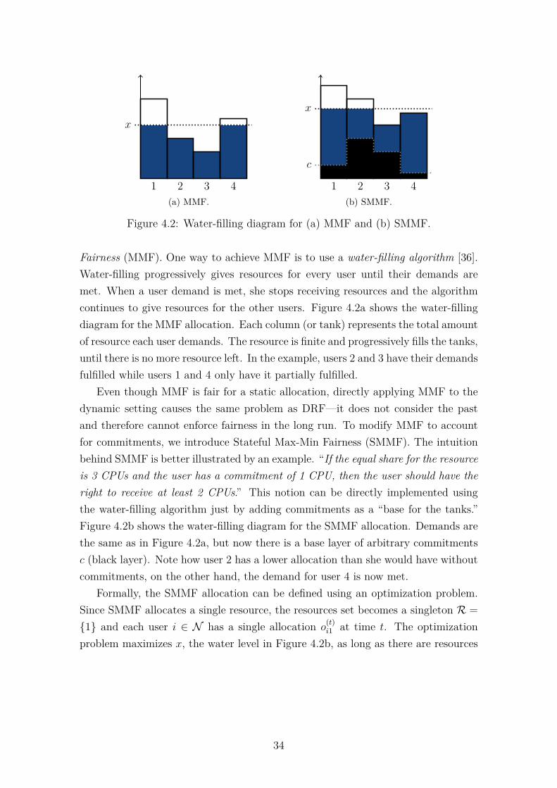
x

1 2 3 4

(a) MMF.

x

c

1 2 3 4

(b) SMMF.

Figure 4.2: Water-filling diagram for (a) MMF and (b) SMMF.

Fairness (MMF). One way to achieve MMF is to use a water-filling algorithm [36].Water-filling progressively gives resources for every user until their demands aremet. When a user demand is met, she stops receiving resources and the algorithmcontinues to give resources for the other users. Figure 4.2a shows the water-fillingdiagram for the MMF allocation. Each column (or tank) represents the total amountof resource each user demands. The resource is finite and progressively fills the tanks,until there is no more resource left. In the example, users 2 and 3 have their demandsfulfilled while users 1 and 4 only have it partially fulfilled.

Even though MMF is fair for a static allocation, directly applying MMF to thedynamic setting causes the same problem as DRF—it does not consider the pastand therefore cannot enforce fairness in the long run. To modify MMF to accountfor commitments, we introduce Stateful Max-Min Fairness (SMMF). The intuitionbehind SMMF is better illustrated by an example. “If the equal share for the resourceis 3 CPUs and the user has a commitment of 1 CPU, then the user should have theright to receive at least 2 CPUs.” This notion can be directly implemented usingthe water-filling algorithm just by adding commitments as a “base for the tanks.”Figure 4.2b shows the water-filling diagram for the SMMF allocation. Demands arethe same as in Figure 4.2a, but now there is a base layer of arbitrary commitmentsc (black layer). Note how user 2 has a lower allocation than she would have withoutcommitments, on the other hand, the demand for user 4 is now met.

Formally, the SMMF allocation can be defined using an optimization problem.Since SMMF allocates a single resource, the resources set becomes a singleton R =

{1} and each user i ∈ N has a single allocation o(t)i1 at time t. The optimization

problem maximizes x, the water level in Figure 4.2b, as long as there are resources

34

left in the system:

maxx

x

s.t.∑i∈N

o(t)i1 ≤ 1,

o(t)i1 = max

{0,min

{θ(t)i1 , (x− c

(t)i1 )}}

.

(4.8)

Given x, each user receives an allocation o(t)i1 = max{0,min{θ(t)i1 , (x − c

(t)i1 )}} which

ensures that allocations are never above demands and remain nonnegative. Whencommitments are zero, SMMF is equivalent to MMF.

Having defined SMMF, we now generalize it to the multiple resources setting tofinally obtain the SDRF mechanism.

4.3.2 SDRF Mechanism

SDRF generalizes SMMF similarly to the way DRF generalizes MMF to multipleresources. We use the same concept of dominant resource as DRF, defined in Eq. 4.3.Differently from DRF, though, we must deal with different commitments for differentresources. We define the dominant commitment for a user i at time t as the user’slargest commitment relative to the system total. As we have normalized all theresources to 1, the dominant commitment is simply the largest commitment for theuser, i.e.,

c(t)i = max

r∈R{c(t)ir } . (4.9)

Having defined the dominant commitment, we define SDRF using ideas fromboth DRF (Eq. 4.5) and SMMF (Eq. 4.8). Like DRF, SDRF increases the share ofdominant resource for every user until a bottleneck is achieved. Like SMMF, usersonly start receiving resources when x is above their (dominant) commitment. SDRFis formally defined as:

maxx

x

s.t.∑i∈N

o(t)ir ≤ 1, ∀r ∈ R ,

o(t)ir = max

{0,min

{θ(t)ir , (x− c

(t)i ) · θ(t)ir

}}.

(4.10)

Recall θ(t)ir is the normalized demand for user i and resource r, defined in Eq. 4.4.From x, we may calculate the allocation for every user and resource by o

(t)ir =

max{0,min{θ(t)ir , (x− c(t)i ) · θ(t)ir }}. In the next subsection we analyze the properties

of SDRF that prove it behaves well in both the stage game and in the long run.

35

4.3.3 Analysis of SDRF Allocation Properties

We start our analysis of SDRF proving that it satisfies the desirable propertiesintroduced in §4.2.2, namely: strategyproofness, Pareto optimality and sharing in-centives. We defer the proofs of all propositions to §4.8.

First, we show that SDRF increases the share of dominant resource for everyuser until a resource runs out (the bottleneck resource). This is indicated in thefollowing proposition.

Proposition 1 (Bottleneck). The SDRF allocation obtained by solving Eq. 4.10is such that all users have their demands fulfilled or there is a bottleneck resource.Formally, o(t)

i = θ(t)i ,∀i ∈ N or ∃r ∈ R such that

∑i∈N o

(t)ir = 1.

Although simple, Proposition 1 is useful to demonstrate the following properties.One of the fundamental properties of DRF is strategyproofness. Without it, usersmay try to manipulate the system by, e.g., faking their usage, which results ininefficiencies [2, 83]. Propositions 2 and 3 show SDRF is also strategyproof.

Proposition 2 (Strategyproofness in the Stage Game). When users consideronly the stage game utility (Eq. 4.1), the SDRF allocation obtained by solving Eq. 4.10is strategyproof.

Proposition 2 shows that when users consider only stage game utilities, SDRFis strategyproof. However, the fact that we consider past allocations may createnew incentives for users to manipulate their declared demands. It may be possiblethat some users would not use the system when they actually need, hoping that thiswould improve their future allocations—this would also bring inefficiencies to thesystem. Fortunately, Proposition 3 shows that this is not possible.

Proposition 3 (Strategyproofness in the Repeated Game). When users eval-uate their utilities using the expected-long-term utility (Eq. 4.2), the SDRF allocationobtained by solving Eq. 4.10 is strategyproof, regardless of users’ discount factors.

The following two propositions demonstrate that SDRF is efficient. Proposition 4shows that SDRF does not waste resources while Proposition 5 shows that theallocation is Pareto optimal, ensuring that it is not possible to increase a user’sallocation without decreasing another.

Proposition 4 (Non-wastefulness). The SDRF allocation O(t) is such that, ifthere is a different allocation O′(t) where o′

(t)ir ≤ o

(t)ir ,∀i ∈ N , r ∈ R and for a

user i∗ ∈ N and resource r∗ ∈ R, o′(t)i∗r∗ < o

(t)i∗r∗, then it must be that u

(t)i∗ (o

(t)i∗ ) >

u(t)i∗ (o

′(t)i∗ ). In other words, SDRF is non-wasteful.

36

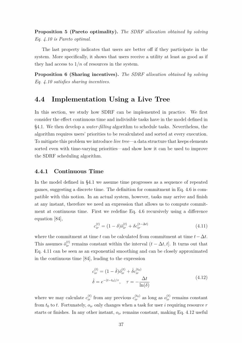
Proposition 5 (Pareto optimality). The SDRF allocation obtained by solvingEq. 4.10 is Pareto optimal.

The last property indicates that users are better off if they participate in thesystem. More specifically, it shows that users receive a utility at least as good as ifthey had access to 1/n of resources in the system.

Proposition 6 (Sharing incentives). The SDRF allocation obtained by solvingEq. 4.10 satisfies sharing incentives.

4.4 Implementation Using a Live TreeIn this section, we study how SDRF can be implemented in practice. We firstconsider the effect continuous time and indivisible tasks have in the model defined in§4.1. We then develop a water-filling algorithm to schedule tasks. Nevertheless, thealgorithm requires users’ priorities to be recalculated and sorted at every execution.To mitigate this problem we introduce live tree—a data structure that keeps elementssorted even with time-varying priorities—and show how it can be used to improvethe SDRF scheduling algorithm.

4.4.1 Continuous Time

In the model defined in §4.1 we assume time progresses as a sequence of repeatedgames, suggesting a discrete time. The definition for commitment in Eq. 4.6 is com-patible with this notion. In an actual system, however, tasks may arrive and finishat any instant, therefore we need an expression that allows us to compute commit-ment at continuous time. First we redefine Eq. 4.6 recursively using a differenceequation [84],

c(t)ir = (1− δ)o

(t)ir + δc

(t−∆t)ir (4.11)

where the commitment at time t can be calculated from commitment at time t−∆t.This assumes o

(t)ir remains constant within the interval (t−∆t, t]. It turns out that

Eq. 4.11 can be seen as an exponential smoothing and can be closely approximatedin the continuous time [84], leading to the expression

c(t)ir = (1− δ)o

(t)ir + δc

(t0)ir

δ = e−(t−t0)/τ , τ = − ∆t

ln(δ)(4.12)

where we may calculate c(t)ir from any previous c

(t0)ir as long as o

(t)ir remains constant

from t0 to t. Fortunately, oir only changes when a task for user i requiring resource r

starts or finishes. In any other instant, oir remains constant, making Eq. 4.12 useful

37

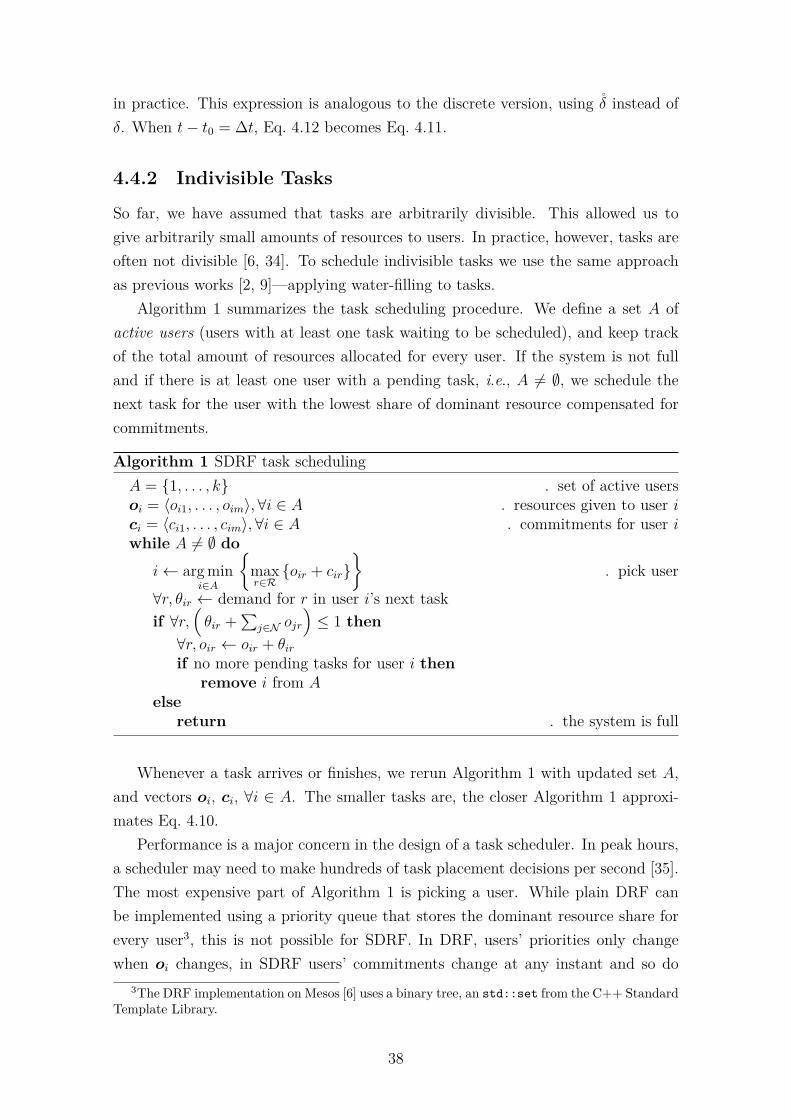
in practice. This expression is analogous to the discrete version, using δ instead ofδ. When t− t0 = ∆t, Eq. 4.12 becomes Eq. 4.11.

4.4.2 Indivisible Tasks

So far, we have assumed that tasks are arbitrarily divisible. This allowed us togive arbitrarily small amounts of resources to users. In practice, however, tasks areoften not divisible [6, 34]. To schedule indivisible tasks we use the same approachas previous works [2, 9]—applying water-filling to tasks.

Algorithm 1 summarizes the task scheduling procedure. We define a set A ofactive users (users with at least one task waiting to be scheduled), and keep trackof the total amount of resources allocated for every user. If the system is not fulland if there is at least one user with a pending task, i.e., A = ∅, we schedule thenext task for the user with the lowest share of dominant resource compensated forcommitments.

Algorithm 1 SDRF task schedulingA = {1, . . . , k} ▷ set of active usersoi = ⟨oi1, . . . , oim⟩,∀i ∈ A ▷ resources given to user ici = ⟨ci1, . . . , cim⟩,∀i ∈ A ▷ commitments for user iwhile A = ∅ do

i← arg mini∈A

{maxr∈R{oir + cir}

}▷ pick user

∀r, θir ← demand for r in user i’s next taskif ∀r,

(θir +

∑j∈N ojr

)≤ 1 then

∀r, oir ← oir + θirif no more pending tasks for user i then

remove i from Aelse

return ▷ the system is full

Whenever a task arrives or finishes, we rerun Algorithm 1 with updated set A,and vectors oi, ci, ∀i ∈ A. The smaller tasks are, the closer Algorithm 1 approxi-mates Eq. 4.10.

Performance is a major concern in the design of a task scheduler. In peak hours,a scheduler may need to make hundreds of task placement decisions per second [35].The most expensive part of Algorithm 1 is picking a user. While plain DRF canbe implemented using a priority queue that stores the dominant resource share forevery user3, this is not possible for SDRF. In DRF, users’ priorities only changewhen oi changes, in SDRF users’ commitments change at any instant and so do

3The DRF implementation on Mesos [6] uses a binary tree, an std::set from the C++ StandardTemplate Library.

38

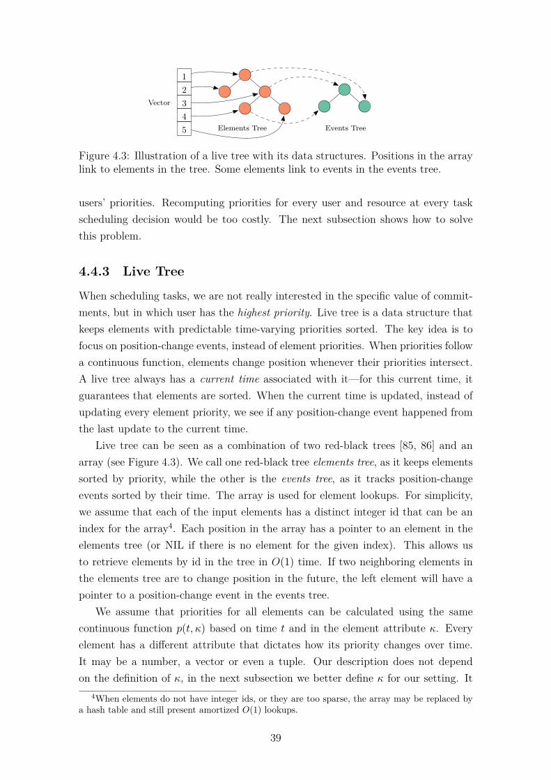
12345

Vector

Elements Tree Events Tree

Figure 4.3: Illustration of a live tree with its data structures. Positions in the arraylink to elements in the tree. Some elements link to events in the events tree.

users’ priorities. Recomputing priorities for every user and resource at every taskscheduling decision would be too costly. The next subsection shows how to solvethis problem.

4.4.3 Live Tree

When scheduling tasks, we are not really interested in the specific value of commit-ments, but in which user has the highest priority. Live tree is a data structure thatkeeps elements with predictable time-varying priorities sorted. The key idea is tofocus on position-change events, instead of element priorities. When priorities followa continuous function, elements change position whenever their priorities intersect.A live tree always has a current time associated with it—for this current time, itguarantees that elements are sorted. When the current time is updated, instead ofupdating every element priority, we see if any position-change event happened fromthe last update to the current time.

Live tree can be seen as a combination of two red-black trees [85, 86] and anarray (see Figure 4.3). We call one red-black tree elements tree, as it keeps elementssorted by priority, while the other is the events tree, as it tracks position-changeevents sorted by their time. The array is used for element lookups. For simplicity,we assume that each of the input elements has a distinct integer id that can be anindex for the array4. Each position in the array has a pointer to an element in theelements tree (or NIL if there is no element for the given index). This allows usto retrieve elements by id in the tree in O(1) time. If two neighboring elements inthe elements tree are to change position in the future, the left element will have apointer to a position-change event in the events tree.

We assume that priorities for all elements can be calculated using the samecontinuous function p(t, κ) based on time t and in the element attribute κ. Everyelement has a different attribute that dictates how its priority changes over time.It may be a number, a vector or even a tuple. Our description does not dependon the definition of κ, in the next subsection we better define κ for our setting. It

4When elements do not have integer ids, or they are too sparse, the array may be replaced bya hash table and still present amortized O(1) lookups.

39

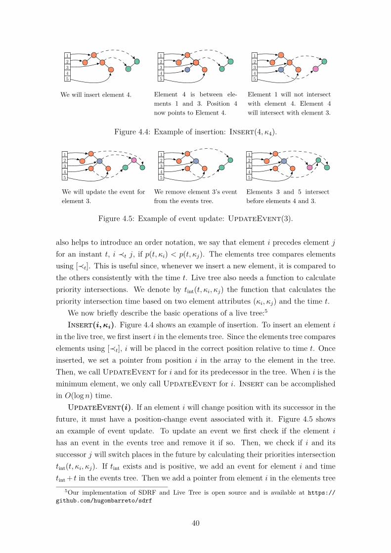
12345

12345

12345

We will insert element 4. Element 4 is between ele-ments 1 and 3. Position 4 now points to Element 4.

Element 1 will not intersect with element 4. Element 4 will intersect with element 3.

Figure 4.4: Example of insertion: Insert(4, κ4).

We will update the event for element 3.

12345

12345

We remove element 3’s event from the events tree.

12345

Elements 3 and 5 intersect before elements 4 and 3.

Figure 4.5: Example of event update: UpdateEvent(3).

also helps to introduce an order notation, we say that element i precedes element j

for an instant t, i ≺t j, if p(t, κi) < p(t, κj). The elements tree compares elementsusing [≺t]. This is useful since, whenever we insert a new element, it is compared tothe others consistently with the time t. Live tree also needs a function to calculatepriority intersections. We denote by tint(t, κi, κj) the function that calculates thepriority intersection time based on two element attributes (κi, κj) and the time t.

We now briefly describe the basic operations of a live tree:5

Insert(i, κi). Figure 4.4 shows an example of insertion. To insert an element iin the live tree, we first insert i in the elements tree. Since the elements tree compareselements using [≺t], i will be placed in the correct position relative to time t. Onceinserted, we set a pointer from position i in the array to the element in the tree.Then, we call UpdateEvent for i and for its predecessor in the tree. When i is theminimum element, we only call UpdateEvent for i. Insert can be accomplishedin O(logn) time.

UpdateEvent(i). If an element i will change position with its successor in thefuture, it must have a position-change event associated with it. Figure 4.5 showsan example of event update. To update an event we first check if the element i

has an event in the events tree and remove it if so. Then, we check if i and itssuccessor j will switch places in the future by calculating their priorities intersectiontint(t, κi, κj). If tint exists and is positive, we add an event for element i and timetint + t in the events tree. Then we add a pointer from element i in the elements tree

5Our implementation of SDRF and Live Tree is open source and is available at https://github.com/hugombarreto/sdrf

40

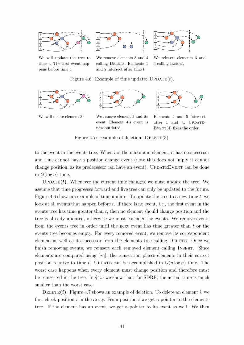
https://github.com/hugombarreto/sdrf

https://github.com/hugombarreto/sdrf

We will update the tree to time t. The first event hap-pens before time t.

12345

We remove elements 3 and 4 calling Delete. Elements 1 and 5 intersect after time t.

We reinsert elements 3 and 4 calling Insert.

t

12345

3 4

12345

t t

Figure 4.6: Example of time update: Update(t).

We will delete element 3.

12345

We remove element 3 and its event. Element 4’s event is now outdated.

Elements 4 and 5 intersect after 1 and 4. Update-Event(4) fixes the order.

12345

12345

Figure 4.7: Example of deletion: Delete(3).

to the event in the events tree. When i is the maximum element, it has no successorand thus cannot have a position-change event (note this does not imply it cannotchange position, as its predecessor can have an event). UpdateEvent can be donein O(logn) time.

Update(t). Whenever the current time changes, we must update the tree. Weassume that time progresses forward and live tree can only be updated to the future.Figure 4.6 shows an example of time update. To update the tree to a new time t, welook at all events that happen before t. If there is no event, i.e., the first event in theevents tree has time greater than t, then no element should change position and thetree is already updated, otherwise we must consider the events. We remove eventsfrom the events tree in order until the next event has time greater than t or theevents tree becomes empty. For every removed event, we remove its correspondentelement as well as its successor from the elements tree calling Delete. Once wefinish removing events, we reinsert each removed element calling Insert. Sinceelements are compared using [≺t], the reinsertion places elements in their correctposition relative to time t. Update can be accomplished in O(n logn) time. Theworst case happens when every element must change position and therefore mustbe reinserted in the tree. In §4.5 we show that, for SDRF, the actual time is muchsmaller than the worst case.

Delete(i). Figure 4.7 shows an example of deletion. To delete an element i, wefirst check position i in the array. From position i we get a pointer to the elementstree. If the element has an event, we get a pointer to its event as well. We then

41

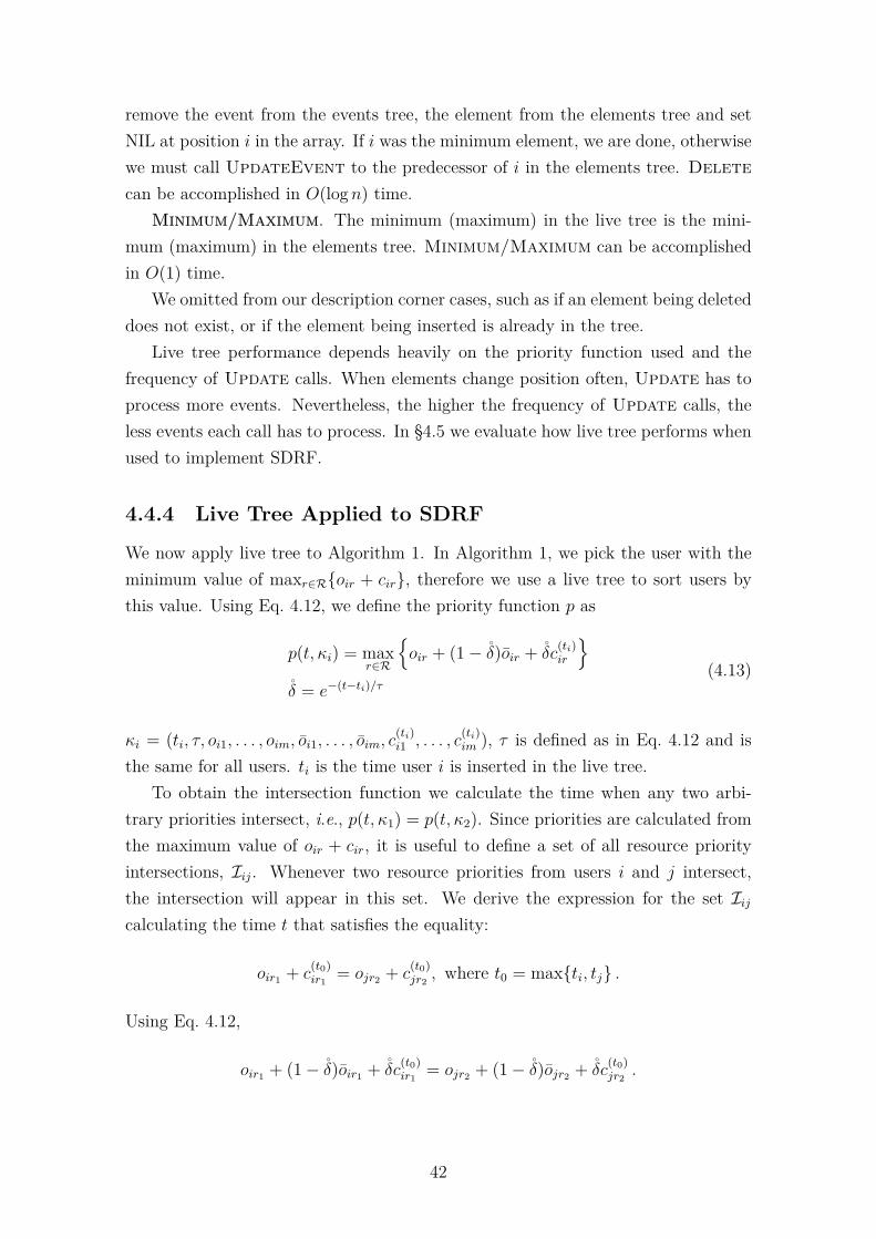
remove the event from the events tree, the element from the elements tree and setNIL at position i in the array. If i was the minimum element, we are done, otherwisewe must call UpdateEvent to the predecessor of i in the elements tree. Deletecan be accomplished in O(logn) time.

Minimum/Maximum. The minimum (maximum) in the live tree is the mini-mum (maximum) in the elements tree. Minimum/Maximum can be accomplishedin O(1) time.

We omitted from our description corner cases, such as if an element being deleteddoes not exist, or if the element being inserted is already in the tree.

Live tree performance depends heavily on the priority function used and thefrequency of Update calls. When elements change position often, Update has toprocess more events. Nevertheless, the higher the frequency of Update calls, theless events each call has to process. In §4.5 we evaluate how live tree performs whenused to implement SDRF.

4.4.4 Live Tree Applied to SDRF

We now apply live tree to Algorithm 1. In Algorithm 1, we pick the user with theminimum value of maxr∈R{oir + cir}, therefore we use a live tree to sort users bythis value. Using Eq. 4.12, we define the priority function p as

p(t, κi) = maxr∈R

{oir + (1− δ)oir + δc

(ti)ir

}δ = e−(t−ti)/τ

(4.13)

κi = (ti, τ, oi1, . . . , oim, oi1, . . . , oim, c(ti)i1 , . . . , c

(ti)im ), τ is defined as in Eq. 4.12 and is

the same for all users. ti is the time user i is inserted in the live tree.To obtain the intersection function we calculate the time when any two arbi-

trary priorities intersect, i.e., p(t, κ1) = p(t, κ2). Since priorities are calculated fromthe maximum value of oir + cir, it is useful to define a set of all resource priorityintersections, Iij. Whenever two resource priorities from users i and j intersect,the intersection will appear in this set. We derive the expression for the set Iijcalculating the time t that satisfies the equality:

oir1 + c(t0)ir1

= ojr2 + c(t0)jr2

, where t0 = max{ti, tj} .

Using Eq. 4.12,

oir1 + (1− δ)oir1 + δc(t0)ir1

= ojr2 + (1− δ)ojr2 + δc(t0)jr2

.

42

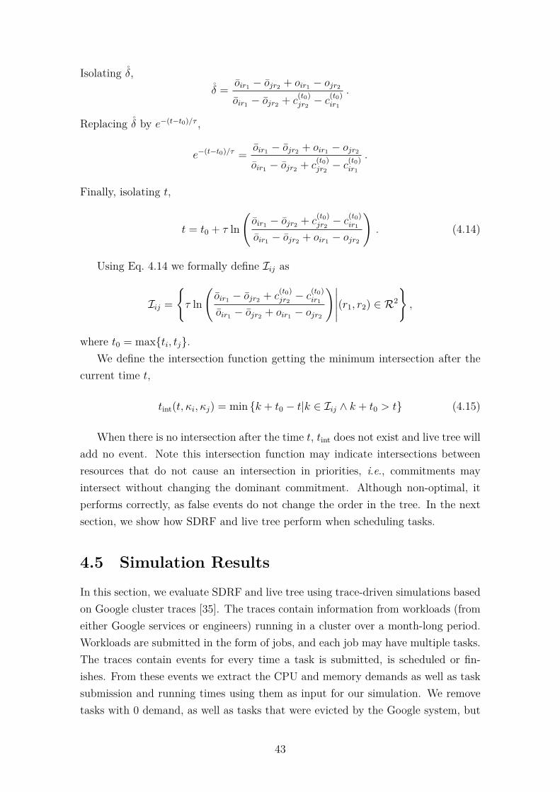
Isolating δ,δ =

oir1 − ojr2 + oir1 − ojr2

oir1 − ojr2 + c(t0)jr2− c

(t0)ir1

.

Replacing δ by e−(t−t0)/τ ,

e−(t−t0)/τ =oir1 − ojr2 + oir1 − ojr2

oir1 − ojr2 + c(t0)jr2− c

(t0)ir1

.

Finally, isolating t,

t = t0 + τ ln(oir1 − ojr2 + c

(t0)jr2− c

(t0)ir1


). (4.14)

Using Eq. 4.14 we formally define Iij as

Iij =

{τ ln

(oir1 − ojr2 + c

(t0)jr2− c

(t0)ir1


)∣∣∣∣∣(r1, r2) ∈ R2

},

where t0 = max{ti, tj}.We define the intersection function getting the minimum intersection after the

current time t,

tint(t, κi, κj) = min {k + t0 − t|k ∈ Iij ∧ k + t0 > t} (4.15)

When there is no intersection after the time t, tint does not exist and live tree willadd no event. Note this intersection function may indicate intersections betweenresources that do not cause an intersection in priorities, i.e., commitments mayintersect without changing the dominant commitment. Although non-optimal, itperforms correctly, as false events do not change the order in the tree. In the nextsection, we show how SDRF and live tree perform when scheduling tasks.

4.5 Simulation ResultsIn this section, we evaluate SDRF and live tree using trace-driven simulations basedon Google cluster traces [35]. The traces contain information from workloads (fromeither Google services or engineers) running in a cluster over a month-long period.Workloads are submitted in the form of jobs, and each job may have multiple tasks.The traces contain events for every time a task is submitted, is scheduled or fin-ishes. From these events we extract the CPU and memory demands as well as tasksubmission and running times using them as input for our simulation. We removetasks with 0 demand, as well as tasks that were evicted by the Google system, but

43

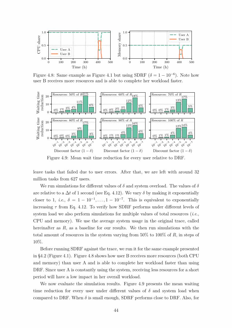
0 100 200 300 400 500

Time (h)

0.0

0.5

1.0

CPU

shar

e

User AUser B

0 100 200 300 400 500

Time (h)

0.0

0.5

1.0

Mem

ory

shar

e User AUser B

Figure 4.8: Same example as Figure 4.1 but using SDRF (δ = 1− 10−6). Note howuser B receives more resources and is able to complete her workload faster.

0

10

20

Wai

ting

time

redu

ctio

n Resources: 50% of R

0% 1% 3% 4%11%

21%

6%

Resources: 60% of R

0% 0% 2% 3%

12%18%

6%

Resources: 70% of R

0% 0% 1% 3%

13%17%

5%

10−1

10−2

10−3

10−4

10−5

10−6

10−7

Discount factor (1− δ)

0

10

20

Wai

ting

time

redu

ctio

n Resources: 80% of R

0% 0% 0% 3%9%

17%

3%

10−1

10−2

10−3

10−4

10−5

10−6

10−7


Resources: 90% of R

0% 1% 1%4%

13%16%

6%

10−1

10−2

10−3

10−4

10−5

10−6

10−7


Resources: 100% of R

0% 1% 1% 4%

12%14%

4%

Figure 4.9: Mean wait time reduction for every user relative to DRF.

leave tasks that failed due to user errors. After that, we are left with around 32million tasks from 627 users.

We run simulations for different values of δ and system overload. The values of δare relative to a ∆t of 1 second (see Eq. 4.12). We vary δ by making it exponentiallycloser to 1, i.e., δ = 1 − 10−1, . . . , 1 − 10−7. This is equivalent to exponentiallyincreasing τ from Eq. 4.12. To verify how SDRF performs under different levels ofsystem load we also perform simulations for multiple values of total resources (i.e.,CPU and memory). We use the average system usage in the original trace, calledhereinafter as R, as a baseline for our results. We then run simulations with thetotal amount of resources in the system varying from 50% to 100% of R, in steps of10%.

Before running SDRF against the trace, we run it for the same example presentedin §4.2 (Figure 4.1). Figure 4.8 shows how user B receives more resources (both CPUand memory) than user A and is able to complete her workload faster than usingDRF. Since user A is constantly using the system, receiving less resources for a shortperiod will have a low impact in her overall workload.

We now evaluate the simulation results. Figure 4.9 presents the mean waitingtime reduction for every user under different values of δ and system load whencompared to DRF. When δ is small enough, SDRF performs close to DRF. Also, for

44

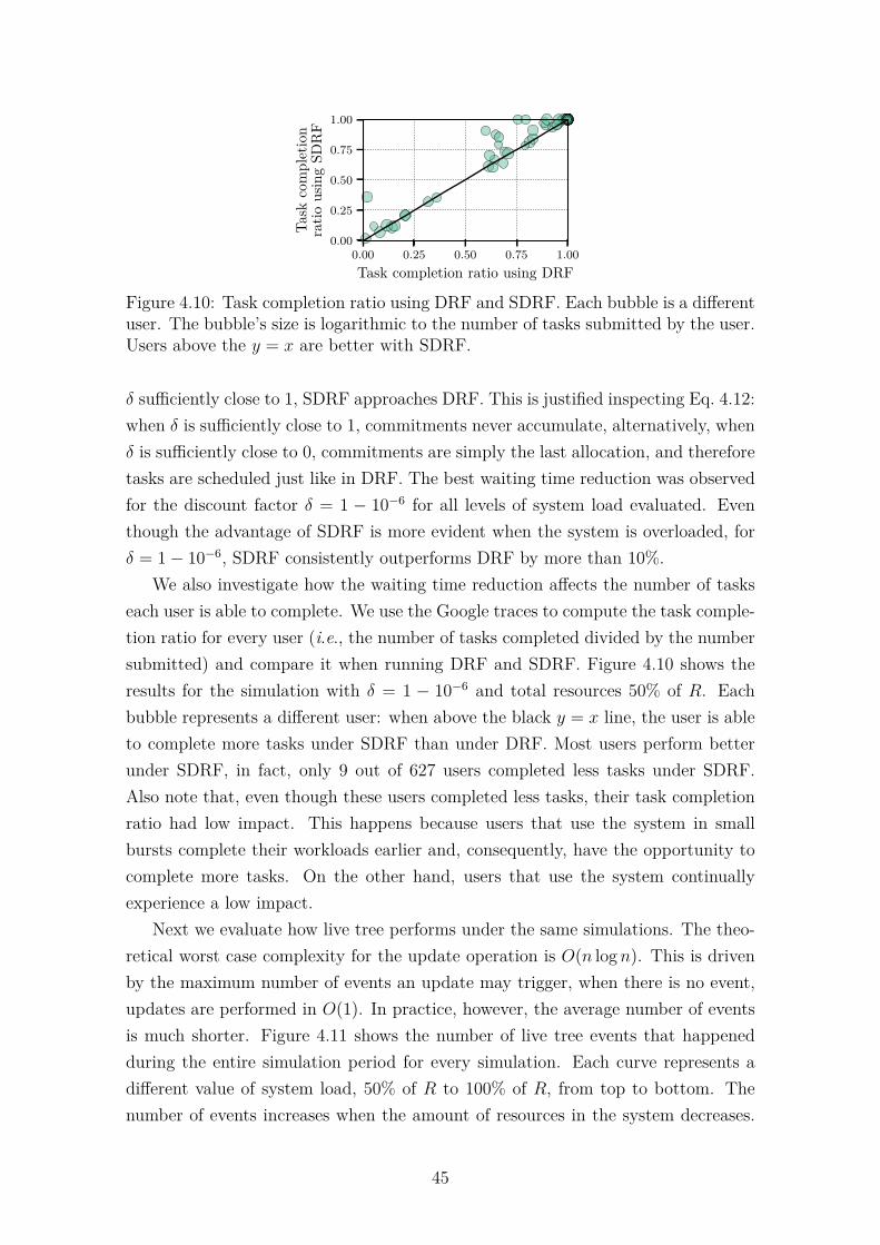
0.00 0.25 0.50 0.75 1.00

Task completion ratio using DRF

0.00

0.25

0.50

0.75

1.00

Task

com

plet

ion

ratio

usin

gSD

RF

Figure 4.10: Task completion ratio using DRF and SDRF. Each bubble is a differentuser. The bubble’s size is logarithmic to the number of tasks submitted by the user.Users above the y = x are better with SDRF.

δ sufficiently close to 1, SDRF approaches DRF. This is justified inspecting Eq. 4.12:when δ is sufficiently close to 1, commitments never accumulate, alternatively, whenδ is sufficiently close to 0, commitments are simply the last allocation, and thereforetasks are scheduled just like in DRF. The best waiting time reduction was observedfor the discount factor δ = 1 − 10−6 for all levels of system load evaluated. Eventhough the advantage of SDRF is more evident when the system is overloaded, forδ = 1− 10−6, SDRF consistently outperforms DRF by more than 10%.

We also investigate how the waiting time reduction affects the number of taskseach user is able to complete. We use the Google traces to compute the task comple-tion ratio for every user (i.e., the number of tasks completed divided by the numbersubmitted) and compare it when running DRF and SDRF. Figure 4.10 shows theresults for the simulation with δ = 1 − 10−6 and total resources 50% of R. Eachbubble represents a different user: when above the black y = x line, the user is ableto complete more tasks under SDRF than under DRF. Most users perform betterunder SDRF, in fact, only 9 out of 627 users completed less tasks under SDRF.Also note that, even though these users completed less tasks, their task completionratio had low impact. This happens because users that use the system in smallbursts complete their workloads earlier and, consequently, have the opportunity tocomplete more tasks. On the other hand, users that use the system continuallyexperience a low impact.

Next we evaluate how live tree performs under the same simulations. The theo-retical worst case complexity for the update operation is O(n logn). This is drivenby the maximum number of events an update may trigger, when there is no event,updates are performed in O(1). In practice, however, the average number of eventsis much shorter. Figure 4.11 shows the number of live tree events that happenedduring the entire simulation period for every simulation. Each curve represents adifferent value of system load, 50% of R to 100% of R, from top to bottom. Thenumber of events increases when the amount of resources in the system decreases.

45

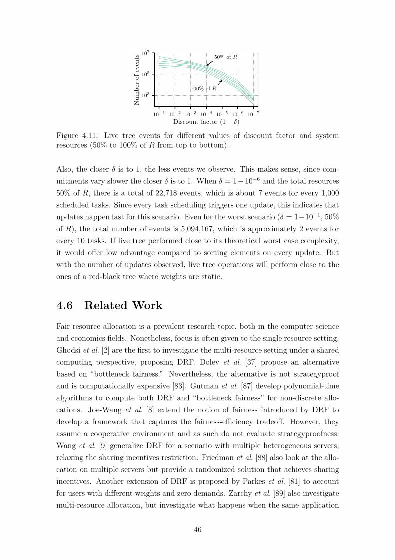
10−1 10−2 10−3 10−4 10−5 10−6 10−7


103

105

107

Num

ber

ofev

ents 50% of R

100% of R

Figure 4.11: Live tree events for different values of discount factor and systemresources (50% to 100% of R from top to bottom).

Also, the closer δ is to 1, the less events we observe. This makes sense, since com-mitments vary slower the closer δ is to 1. When δ = 1−10−6 and the total resources50% of R, there is a total of 22,718 events, which is about 7 events for every 1,000

scheduled tasks. Since every task scheduling triggers one update, this indicates thatupdates happen fast for this scenario. Even for the worst scenario (δ = 1−10−1, 50%of R), the total number of events is 5,094,167, which is approximately 2 events forevery 10 tasks. If live tree performed close to its theoretical worst case complexity,it would offer low advantage compared to sorting elements on every update. Butwith the number of updates observed, live tree operations will perform close to theones of a red-black tree where weights are static.

4.6 Related WorkFair resource allocation is a prevalent research topic, both in the computer scienceand economics fields. Nonetheless, focus is often given to the single resource setting.Ghodsi et al. [2] are the first to investigate the multi-resource setting under a sharedcomputing perspective, proposing DRF. Dolev et al. [37] propose an alternativebased on “bottleneck fairness.” Nevertheless, the alternative is not strategyproofand is computationally expensive [83]. Gutman et al. [87] develop polynomial-timealgorithms to compute both DRF and “bottleneck fairness” for non-discrete allo-cations. Joe-Wang et al. [8] extend the notion of fairness introduced by DRF todevelop a framework that captures the fairness-efficiency tradeoff. However, theyassume a cooperative environment and as such do not evaluate strategyproofness.Wang et al. [9] generalize DRF for a scenario with multiple heterogeneous servers,relaxing the sharing incentives restriction. Friedman et al. [88] also look at the allo-cation on multiple servers but provide a randomized solution that achieves sharingincentives. Another extension of DRF is proposed by Parkes et al. [81] to accountfor users with different weights and zero demands. Zarchy et al. [89] also investigatemulti-resource allocation, but investigate what happens when the same application

46

may be developed differently to use different proportions of resource types. Theypropose a framework that allows users to submit multiple demands for the sameapplication. Even though the aforementioned works consider the multi-resourcesetting, they ignore the dynamic nature of users’ demands.

Bonald and Roberts [38] suggest Bottleneck Max Fairness (BMF), which alsodoes not enforce strategyproofness, but improves resource utilization as comparedto DRF. They consider dynamic demands in their analysis, arguing that for highlydynamic environments, such as networks, it is hard for users to manipulate thesystem. BMF convergence is proved in a later work [90]. Even though the analysisof BMF considers dynamic demands, the allocation itself considers only short termusage, ignoring fairness in the long run. Kash et al. [82] investigate a dynamic settingwhere users arrive and never leave, however, they also assume that demands remainconstant. Friedman et al. [91] evaluate the scenario where multiple users arrive andleave the system. The focus, however, is on the fair division of resources as soon asthe user arrives, limiting the number of task disruptions. There are also works thatadapt DRF to packet processing [83, 92] and consider a recent past. Nevertheless,this is done to prevent limitations that arise when scheduling packets—in whichresources must be shared in time—and not to ensure fairness and efficiency in thelong run. Finally, other authors have focused on improving efficiency in the longrun but not fairness [4, 93]. While some of these works consider users’ dynamicity,they do not address fairness in the long run, which was our focus in this chapter.

Live Tree can be seen as an alternative implementation of a Kinetic PriorityQueue [94]. Different from the classical implementations, however, Live Tree en-sures strict upper bounds for priorities that follow an arbitrary continuous function.This happens because, in the classical implementations, elements are swapped—orrotated—in the presence of events [95]. Live Tree does not swap elements, instead,it removes pair of elements and reinsert them according to the update time t. Bydoing this, it ensures that every update has a cost of O(logn) for every changingpair of elements, regardless of the number of intersections that happen from the lastupdate to the current. This is particularly useful for SDRF, since the function thatcalculates weights is not trivial (Eq. 4.15).

4.7 ConclusionIn this chapter, we introduced SDRF, an extension of DRF that enforces fairness inthe long run. SDRF looks at past allocations and benefits users with lower averageusage. We showed that SDRF satisfies the fundamental properties of DRF whileenforcing fairness in the long run. To efficiently implement SDRF, we introducedlive tree, a general-purpose data structure that keeps elements with predictable

47

time-varying priorities sorted. We simulated SDRF using Google cluster traces for amonth-long period. Results have shown that under SDRF, users with low utilizationcan complete their workloads faster. Meanwhile, users with high utilization suffer alow impact in their overall workload. We also used the simulations to evaluate livetree performance, concluding that SDRF can be implemented efficiently.

There are different future investigation directions. First, we believe live tree maybenefit other applications, e.g., Dijkstra’s algorithm applied to graphs with time-variable weights. Second, SDRF can be extended to cover other applications, e.g.,collaborative clouds [96]. Moreover, although we mentioned the possibility of usingweights for users, we did not evaluate it formally. Another possibility is the use ofa different function to measure commitments.

4.8 Deferred ProofsIn this section, we prove the propositions stated in §4.3.3. Before continuing, weintroduce a simple lemma. This lemma states that the allocation a user gets for acertain resource will always be the normalized demand for this resource multipliedby the allocation for the dominant resource. For example, if the normalized demandvector for a user is ⟨0.5, 1⟩ and the allocation for the dominant resource is 0.2, then,the allocation would be ⟨0.1, 0.2⟩.

Lemma 1. Given an SDRF allocation O(t), obtained by solving Eq. 4.10, the al-location user i receives for resource r is such that o

(t)ir = θ

(t)ir o

(t)

ir(t)i

,∀i ∈ N , r ∈ R.

Proof. The proof is straightforward. From Eq. 4.10 we know that o(t)ir ∈ [0, θ

(t)ir ].

• When o(t)ir ∈ (0, θ

(t)ir ):

o(t)ir = (x− c

(t)i ) · θ(t)ir . (4.16)

By replacing x− c(t)i = o

(t)ir /θ

(t)ir in Eq. 4.10, and as long as o

ir(t)i∈ (0, θ

(t)

ir(t)i

), weget to

o(t)

ir(t)i

= o(t)ir /θ

(t)ir ,

therefore,o(t)ir = θ

(t)ir o

(t)

ir(t)i

. (4.17)

Thus we just need to prove that o(t)

ir(t)i

∈ (0, θ(t)

ir(t)i

). In fact, o(t)ir

(t)i

> 0, since we

are considering o(t)ir > 0 and by definition θ

(t)

ir(t)i

> 0. Verifying the upper bound

is also straightforward. We depart from o(t)ir < θ

(t)ir and use the definition in

Eq. 4.4,θ(t)ir θ

(t)

ir(t)i

> o(t)ir

48

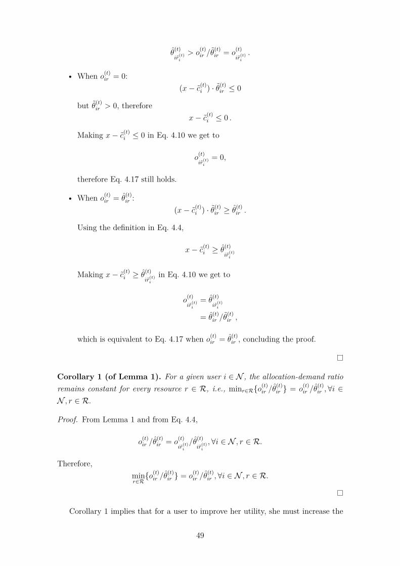
θ(t)

ir(t)i

> o(t)ir /θ

(t)ir = o

(t)

ir(t)i

.

• When o(t)ir = 0:

(x− c(t)i ) · θ(t)ir ≤ 0

but θ(t)ir > 0, therefore

x− c(t)i ≤ 0 .

Making x− c(t)i ≤ 0 in Eq. 4.10 we get to

o(t)

ir(t)i

= 0,

therefore Eq. 4.17 still holds.

• When o(t)ir = θ

(t)ir :

(x− c(t)i ) · θ(t)ir ≥ θ

(t)ir .

Using the definition in Eq. 4.4,

x− c(t)i ≥ θ

(t)

ir(t)i

Making x− c(t)i ≥ θ

(t)

ir(t)i

in Eq. 4.10 we get to

o(t)

ir(t)i

= θ(t)

ir(t)i

= θ(t)ir /θ

(t)ir ,

which is equivalent to Eq. 4.17 when o(t)ir = θ

(t)ir , concluding the proof.

Corollary 1 (of Lemma 1). For a given user i ∈ N , the allocation-demand ratioremains constant for every resource r ∈ R, i.e., minr∈R{o(t)ir /θ

(t)ir } = o

(t)ir /θ

(t)ir ,∀i ∈

N , r ∈ R.

Proof. From Lemma 1 and from Eq. 4.4,

o(t)ir /θ

(t)ir = o

(t)

ir(t)i

/θ(t)

ir(t)i

,∀i ∈ N , r ∈ R.

Therefore,minr∈R{o(t)ir /θ

(t)ir } = o

(t)ir /θ

(t)ir ,∀i ∈ N , r ∈ R.

Corollary 1 implies that for a user to improve her utility, she must increase the

49

allocation for every resource, otherwise the minimum allocation-demand ratio wouldnot change.

We now turn to the proof of Proposition 1. It shows that if a user did not haveher demand fulfilled, there must be at least one resource that is fully utilized—abottleneck resource.

Proposition 1 (Bottleneck). The SDRF allocation obtained by solving Eq. 4.10is such that all users have their demands fulfilled or there is a bottleneck resource.Formally, o(t)

i = θ(t)i ,∀i ∈ N or ∃r ∈ R such that

∑i∈N o

(t)ir = 1.

Proof. Assume, by way of contradiction, that we can obtain an allocation O(t) fromEq. 4.10 where ∃i ∈ N such that o

(t)i = θ

(t)i and

∑i∈N o

(t)ir = 1,∀r ∈ R.

First, from the problem restrictions in Eq. 4.10, we know that o(t)ir ≤ θ

(t)ir ,∀i ∈

N , r ∈ R and∑

i∈N o(t)ir ≤ 1,∀r ∈ R. Thus,∑

i∈N

o(t)ir < 1, ∀r ∈ R and (4.18)

∃i ∈ N , r ∈ R such that o(t)ir < θ

(t)ir . (4.19)

We now verify if we can propose a different solution to the problem:

x′ = x+ ϵ, ϵ ∈ R+.

If we can find a positive ϵ in which x′ satisfies the problem constraints this is acontradiction (since x′ > x it could have been a solution to Eq. 4.10 instead of x).We denote by O′(t) the allocation found using x′. If we can obtain a positive ϵ thatsatisfies the constraints, the following expression should hold,∑

i∈N

o′(t)ir ≤

∑i∈N

(o(t)ir + ϵ θ

(t)ir

)≤ 1,∀r ∈ R .

Therefore,

ϵ ≤ minr∈R

{1−

∑i∈N o

(t)ir∑

i∈N θ(t)ir

}.

Since we want ϵ > 0, we need to prove that

minr∈R

{1−

∑i∈N o

(t)ir∑

i∈N θ(t)ir

}> 0.

From Eq. 4.18, we know that

1−∑i∈N

o(t)ir > 0,∀r ∈ R.

50

Therefore we need to verify if ∑i∈N

θ(t)ir > 0,∀r ∈ R,

which is also true since θ(t)ir > 0,∀i ∈ N , r ∈ R. Thus we can find an ϵ > 0, making

x′ > x, which is a contradiction.

Proposition 2 (Strategyproofness in the Stage Game). When users consideronly the stage game utility (Eq. 4.1), the SDRF allocation obtained by solving Eq. 4.10is strategyproof.

Proof. Take an arbitrary user j ∈ N , we denote the allocation returned by themechanism for the user j when θj = θj by oj, and when θj = θj by o′

j. We mustprove that

uj(oj) ≥ uj(o′j) . (4.20)

We check the following three cases.

• When uj(oj) = 1: the utility cannot be improved and Eq. 4.20 trivially holds.

• When uj(oj) = 0: from Corollary 1, ojr = 0,∀r ∈ R. Therefore x−cj ≤ 0, andthe allocation is zero for any resource, independently from θj, which makesEq. 4.20 true.

• When 0 < uj(oj) < 1: for this case, allocations are not limited by θj. We maysimplify the expression for the allocation in Eq. 4.10

ojr = (x− cj) · θjr .

From Proposition 1 there is a bottleneck resource, and we denote it as r∗.From Corollary 1 users must increase the allocation for all resources in orderto improve their utilities. Therefore, if we can prove that it is impossibleto have an alternative demand vector that increases the share of both thebottleneck resource and the dominant resource, we are done.

We denote by θj the truthful normalized demand vector for user j, and by θ′j,

the misreported normalized demand for user j.

Increasing the share of dominant resource: The share of dominant re-source user j receives when declaring the truth is given by:

ojrj = (x− cj) · θjrj = x− cj.

51

Therefore, to increase the share of dominant resource for user j (i.e., makeo′jrj > ojrj), we must make x′ > x, where x′ is the solution to Eq. 4.10 whenuser j declares θ′

j instead of θj.

Increasing the share of bottleneck resource: Since r∗ is a bottleneckresource, the following holds:

ojr∗ +∑

i∈N\{j}

oir∗ = 1

Therefore, to make o′jr∗ > ojr∗ , we must decrease the sum of allocations of allusers but j: ∑

i∈N\{j}

o′ir∗ <∑

i∈N\{j}

oir∗

and, consequently, since r∗ is a bottleneck resource,∑i∈N\{j}

(x′ − ci)θir∗ <∑

i∈N\{j}

(x− ci)θir∗

∑i∈N\{j}

(x′ − ci) <∑

i∈N\{j}

(x− ci)

x′ < x

Since increasing the share of dominant resource requires x′ > x, while in-creasing the share of bottleneck resource requires x′ < x, it is not possible toincrease both shares, which concludes the proof.

Proposition 3 (Strategyproofness in the Repeated Game). When users eval-uate their utilities using the expected-long-term utility (Eq. 4.2), the SDRF allocationobtained by solving Eq. 4.10 is strategyproof, regardless of users’ discount factors.

Proof. Take an arbitrary user i ∈ N , assuming user i discounts her utility usingδi and the allocation mechanism calculates commitments using δ. Without loss ofgenerality, we represent the expected-long-term utility for time t = 0 by

u[0,∞)i = Eui

[(1− δi)

∞∑k=0

δki u(k)i (o

(k)i )

]. (4.21)

Since manipulating the stage game is not possible, the only hope users may haveof improving their expected-long-term utility is by reducing their commitments. Toreduce their commitments, users may declare a lower demand. We will show thatany marginal gain the user may get, does not compensate her loss in the stage game.

52

If a user i declares a demand θ(0)ir = θ

(0)ir − ϵ, with 0 < ϵ < θ

(0)ir , for a resource r,

in the best scenario, this will make user i’s commitment

c′(k)ir = c

(k)ir − (1− δ)δkϵ, (4.22)

where c′(k)ir is the new commitment user i gets by declaring θ

(0)ir . From this commit-

ment, the maximum possible improvement in the long-term utility is

u[0,∞)i = −(1− δi)ϵ+ (1− δi)

∞∑k=1

δki (1− δ)δkϵ

= −ϵ(1− δi) + ϵ(1− δi)(1− δ)∞∑k=1

(δi · δ)k.

Then, replacing the infinite series,

u[0,∞)i = −ϵ(1− δi) + ϵ(1− δi)(1− δ)

(1

1− δi · δ− 1

)= ϵ(1− δi)

((1− δ)

1− δi · δ− (1− δ)− 1

).

Inspecting the expression we verify that, for 0 ≤ δ < 1 and 0 ≤ δi < 1,

(1− δ)

1− δi · δ< (1− δ) + 1

and therefore,u[0,∞)i < 0 .

Thus, any positive decrement ϵ in the declared demands cannot possibly improvethe expected-long-term utility, independently from users discount factors.

Proposition 4 (Non-wastefulness). The SDRF allocation O(t) is such that, ifthere is a different allocation O′(t) where o′

(t)ir ≤ o

(t)ir ,∀i ∈ N , r ∈ R and for a

user i∗ ∈ N and resource r∗ ∈ R, o′(t)i∗r∗ < o

(t)i∗r∗, then it must be that u

(t)i∗ (o

(t)i∗ ) >

u(t)i∗ (o

′(t)i∗ ). In other words, SDRF is non-wasteful.

Proof. Assuming truthful demands, using Corollary 1 and the definition in Eq. 4.1,we have

u(t)i (o

(t)i ) = o

(t)ir /θ

(t)ir ,∀i ∈ N , r ∈ R .

Using the definition of O′(t),

o′(t)i∗r∗/θ

(t)i∗r∗ < o

(t)i∗r∗/θ

(t)i∗r∗ = u

(t)i∗ (o

(t)i∗ ).

53

However,

u(t)i∗ (o

′(t)i∗ ) = min

{minr∈R{o′(t)i∗r/θ

(t)i∗r}, 1

}≤ o′

(t)i∗r∗/θ

(t)i∗r∗ .

Therefore,u(t)i∗ (o

′(t)i∗ ) < u

(t)i∗ (o

(t)i∗ ),

concluding the proof.

Proposition 5 (Pareto optimality). The SDRF allocation obtained by solvingEq. 4.10 is Pareto optimal.

Proof. The proof is a direct consequence of Propositions 1 and 4. For the sake ofcontradiction, assume SDRF is not Pareto optimal, then, from the allocation O(t)

obtained by solving Eq. 4.10 we can get another allocation O′(t) that makes a useri∗ ∈ N strictly better while making everybody’s utility at least as good, i.e.,

u(t)i∗ (o

′(t)i∗ ) > u

(t)i∗ (o

(t)i∗ ) and (4.23)

∀i ∈ N , u(t)i (o

′(t)i ) ≥ u

(t)i (o

(t)i ). (4.24)

From Proposition 4, if ∃i ∈ N , r ∈ R such that o′(t)ir < o

(t)ir , then u

(t)i (o

′(t)i ) <

u(t)i (o

(t)i ). Therefore we may rewrite Eq. 4.24 as

o′(t)ir ≥ o

(t)ir , ∀i ∈ N , r ∈ R. (4.25)

Also, from Corollary 1, we know that we must increase the allocation for all resourcesin order to increase the utility of a user, i.e., for the user i∗,

o′(t)i∗r > o

(t)i∗r,∀r ∈ R.

From Proposition 1, either

o(t)i = θ

(t)i or (4.26)

∃r∗ ∈ R such that∑i∈N

o(t)ir∗ = 1 . (4.27)

If Eq. 4.26 is true, then u(t)i (o

(t)i ) = 1,∀i ∈ N and Eq. 4.23 cannot be true. Therefore

Eq. 4.27 must be true. But since Eq. 4.27 is true, when we make o′(t)i∗r∗ > o

(t)i∗r∗ , we

must decrease the allocation of another user, contradicting Eq. 4.25.

Proposition 6 (Sharing incentives). The SDRF allocation obtained by solvingEq. 4.10 satisfies sharing incentives.

54

Proof. To prove sharing incentives, it is sufficient to show that there is a strategy,user i may follow, which makes her utility at least as good as u

(t)i (⟨1/n, . . . , 1/n⟩),

regardless of other users actions. We show that the strategy “always declare θ(t)i =

⟨1/n, . . . , 1/n⟩” guarantees that o(t)i = ⟨1/n, . . . , 1/n⟩ for every instant t.

From Eq. 4.10, o(t)ir ≤ θ(t)ir for every r ∈ R, therefore, o(t)ir ≤ 1/n. From Eq. 4.6,

this makes c(t)ir = 0 for every resource r and instant t, also making c

(t)i = 0 (from

Eq. 4.9). Since c(t)i = 0, the allocation received by i will be o

(t)ir = min{x, 1/n} for

every resource r and instant t. Nevertheless, x ≥ 1/n, which makes o(t)ir = 1/n,

concluding the proof.

55

Chapter 5

Conclusions and the Future ofNetworks and Datacenters

In this thesis, we have looked at ways of improving efficiency and fairness on twodistinct shared systems: software middleboxes and datacenters. In this final chapterwe summarize our contributions and propose directions for future work.

In Chapter 3 we took inspiration from modern datacenter networks and hypoth-esized that multi-core software middleboxes could also benefit from load-balancingpackets at a finer granularity than flows. To validate this hypothesis we designedand implemented Sprayer. Sprayer not only configures the NIC to send packetsfrom the same flow to multiple cores, but also provides abstractions for handlingflow state in such context. We verified that, for the number of concurrent flows typ-ical of real workloads, Sprayer improves fairness and TCP throughput even thoughit reorders packets.

In Chapter 4 we departed from the observation that current task schedulers donot ensure fairness in the long run. This ends up benefiting users with long-runningjobs more than users that use the system sporadically. With SDRF, we showedthat it is possible to allocate tasks more efficiently and improve long-term fairnessby considering past allocations. To efficiently implement SDRF we also proposedlive tree, a new data structure that keeps elements with predictable time-varyingpriorities sorted. We proved SDRF keeps the same fundamental properties of DRFand used trace-driven simulations to show that it reduces the waiting time for low-demand users, while having a low impact on high-demand users.

Before finishing, we highlight trends in hardware and applications that are likelyto affect both networks and schedulers. Moreover, we point to problems and oppor-tunities that are consequence of these trends.

56

5.1 Domain-Specific ArchitecturesIn the last decades, CPUs obtained orders-of-magnitude performance improvementsfrom architecture innovations, such as out-of-order execution and caches, as well asfrom Moore’s Law.1 Moore’s Law, however, is coming to an end, and in the last fewyears hardware architects have been struggling to achieve even small performanceimprovements [97]. In response to this limitation, chip designers now widely believethat to continue to increase performance, while still providing programmability,there must be a move towards Domain-Specific Architectures (DSAs) [97]. DSAsare specialized chips that are less flexible than general-purpose CPUs but moreefficient in their domains. Note that DSAs are different from strict ASICs, sinceDSAs serve not one, but a domain of applications. A recent example of DSA isGoogle’s Tensor Processing Unit (TPU) that runs deep neural networks 15 to 30times faster than contemporary CPUs [98].

If the DSA trend continues, datacenters are likely to have multiple types ofspecialized chips to accommodate different application domains. In such a setting,schedulers must be able to decide which tasks will use specialized chips and whichwill run on general-purpose CPUs. As is the case today with GPUs, some taskswill benefit more from running on DSAs than others. Designing a scheduler thattakes this into account while ensuring the properties listed in §2.2.1 is an interestingresearch direction.

DSAs are also starting to appear in networks, with a movement towards pro-grammable NICs [73, 74] and switches [99–102]. Programmable NICs and switchesnot only speedup the deployment of new protocols but also open new avenues forimproving congestion control and packet scheduling. In §3.5 we have discussed afew ways in which programmable NICs could be used to improve Sprayer, but weexpect to see many other applications.

5.2 Decentralized Control and ComputationRecently, there has been a surge of applications with decentralized control and com-putation. For instance, fog computing—a move of the cloud computing paradigm tothe edge of the network—is gaining traction as a way of fulfilling the latency, mo-bility and scalability requirements of the Internet of Things [103, 104]. A schedulerfor the fog must also take these requirements into consideration.

Another increasingly popular set of applications with decentralized control andcomputation are cryptocurrencies. Cryptocurrencies make use of a distributed ledgerto record transactions and avoid double spending. One of the side effects of the

1Moore’s law states that the number of transistors per chip doubles every one or two years.

57

increase popularity of cryptocurrencies is the potential to change incentives in sharedcomputing systems. With cryptocurrencies, any spare computation can be used formining. This has already become a problem, with some websites and apps miningcryptocurrency on users’ computers and phones [105]. In shared datacenters withina company or lab, users may suffer retaliation for doing this, but in a less restrictivecollaborative environment, users have incentives to turn spare capacity into profit.In this scenario, the idea of considering long-term fairness introduced in Chapter 4may also be explored to help solving this problem.

58

Bibliography

[1] JAFFE, J., “Bottleneck Flow Control,” IEEE Transactions on Communications,v. 29, n. 7, pp. 954–962, Jul. 1981.

[2] GHODSI, A., ZAHARIA, M., HINDMAN, B., et al., “Dominant Resource Fair-ness: Fair Allocation of Multiple Resource Types.” In: Proceedings of the8th USENIX Symposium on Networked Systems Design and Implementa-tion, NSDI ’11, pp. 323–336, Mar. 2011.

[3] CHOWDHURY, M., ZHONG, Y., STOICA, I., “Efficient Coflow Schedulingwith Varys.” In: Proceedings of the Conference of the ACM Special InterestGroup on Data Communication, SIGCOMM ’14, pp. 443–454, Aug. 2014.

[4] GRANDL, R., CHOWDHURY, M., AKELLA, A., et al., “Altruistic Schedulingin Multi-Resource Clusters.” In: Proceedings of the 12th USENIX Sym-posium on Operating Systems Design and Implementation, OSDI ’16, pp.65–80, Nov. 2016.

[5] PROCACCIA, A. D., “Cake Cutting: Not Just Child’s Play,” Communicationsof the ACM, v. 56, n. 7, pp. 78–87, Jul. 2013.

[6] HINDMAN, B., KONWINSKI, A., ZAHARIA, M., et al., “Mesos: A Platformfor Fine-Grained Resource Sharing in the Data Center.” In: Proceedingsof the 8th USENIX Symposium on Networked Systems Design and Imple-mentation, NSDI ’11, pp. 295–308, Mar. 2011.

[7] JAIN, R. K., CHIU, D.-M. W., HAWE, W. R., “A Quantitative Measure ofFairness and Discrimination for Resource Allocation in Shared ComputerSystems.” Technical Report DEC-TR-301, Eastern Research Laboratory,Digital Equipment Corporation, Hudson, MA, Sep. 1984.

[8] JOE-WONG, C., SEN, S., LAN, T., et al., “Multiresource Allocation: Fairnes-Efficiency Tradeoffs in a Unifying Framework,” IEEE/ACM Transactionson Networking, v. 21, n. 6, pp. 1785–1798, Dec. 2013.

59

[9] WANG, W., LI, B., LIANG, B., “Dominant Resource Fairness in Cloud Com-puting Systems with Heterogeneous Servers.” In: Proceedings of the IEEEConference on Computer Communications, INFOCOM 2014, pp. 583–591, Apr. 2014.

[10] DIXIT, A., PRAKASH, P., HU, Y. C., et al., “On the Impact of Packet Spray-ing in Data Center Networks.” In: Proceedings of the IEEE Conference onComputer Communications, INFOCOM 2013, pp. 2130–2138, Apr. 2013.

[11] SEKAR, V., EGI, N., RATNASAMY, S., et al., “Design and Implementationof a Consolidated Middlebox Architecture.” In: Proceedings of the 9thUSENIX Symposium on Networked Systems Design and Implementation,NSDI ’12, pp. 323–336, Apr. 2012.

[12] SHERRY, J., HASAN, S., SCOTT, C., et al., “Making Middleboxes SomeoneElse’s Problem: Network Processing as a Cloud Service.” In: Proceedingsof the Conference of the ACM Special Interest Group on Data Communi-cation, SIGCOMM ’12, pp. 13–24, Aug. 2012.

[13] CHIOSI, M., CLARKE, D., PETER WILLIS, A. R., et al., “Network FunctionsVirtualisation: An Introduction, Benefits, Enablers, Challenges & Callfor Action.” Technical report, European Telecommunications StandardsInstitute, Oct. 2012. Available at: <https://portal.etsi.org/NFV/NFV_White_Paper.pdf>.

[14] HWANG, J., RAMAKRISHNAN, K. K., WOOD, T., “NetVM: High Perfor-mance and Flexible Networking Using Virtualization on Commodity Plat-forms.” In: Proceedings of the 11th USENIX Symposium on NetworkedSystems Design and Implementation, NSDI ’14, pp. 445–458, Apr. 2014.

[15] KATSIKAS, G. P., BARBETTE, T., KOSTIĆ, D., et al., “Metron: NFV Ser-vice Chains at the True Speed of the Underlying Hardware.” In: Proceed-ings of the 15th USENIX Symposium on Networked Systems Design andImplementation, NSDI ’18, pp. 171–186, Apr. 2018.

[16] KULKARNI, S. G., ZHANG, W., HWANG, J., et al., “NFVnice: DynamicBackpressure and Scheduling for NFV Service Chains.” In: Proceedings ofthe Conference of the ACM Special Interest Group on Data Communica-tion, SIGCOMM ’17, pp. 71–84, Aug. 2017.

[17] PALKAR, S., LAN, C., HAN, S., et al., “E2: A Framework for NFV Appli-cations.” In: Proceedings of the 25th Symposium on Operating SystemsPrinciples, SOSP ’15, pp. 121–136, Oct. 2015.

60

https://portal.etsi.org/NFV/NFV_White_Paper.pdf

https://portal.etsi.org/NFV/NFV_White_Paper.pdf

[18] SHERRY, J., GAO, P. X., BASU, S., et al., “Rollback-Recovery for Middle-boxes.” In: Proceedings of the Conference of the ACM Special InterestGroup on Data Communication, SIGCOMM ’15, pp. 227–240, Aug. 2015.

[19] SUN, C., BI, J., ZHENG, Z., et al., “NFP: Enabling Network Function Par-allelism in NFV.” In: Proceedings of the Conference of the ACM SpecialInterest Group on Data Communication, SIGCOMM ’17, pp. 43–56, Aug.2017.

[20] TOOTOONCHIAN, A., PANDA, A., LAN, C., et al., “ResQ: Enabling SLOsin Network Function Virtualization.” In: Proceedings of the 15th USENIXSymposium on Networked Systems Design and Implementation, NSDI ’18,pp. 283–297, Apr. 2018.

[21] BARI, F., CHOWDHURY, S. R., AHMED, R., et al., “Orchestrating Virtu-alized Network Functions,” IEEE Transactions on Network and ServiceManagement, v. 13, n. 4, pp. 725–739, Dec. 2016.

[22] GEMBER-JACOBSON, A., VISWANATHAN, R., PRAKASH, C., et al.,“OpenNF: Enabling Innovation in Network Function Control.” In: Pro-ceedings of the Conference of the ACM Special Interest Group on DataCommunication, SIGCOMM ’14, pp. 163–174, Aug. 2014.

[23] KABLAN, M., ALSUDAIS, A., KELLER, E., et al., “Stateless Network Func-tions: Breaking the Tight Coupling of State and Processing.” In: Proceed-ings of the 14th USENIX Symposium on Networked Systems Design andImplementation, NSDI ’17, pp. 97–112, Mar. 2017.

[24] RAJAGOPALAN, S., WILLIAMS, D., JAMJOOM, H., et al., “Split/Merge:System Support for Elastic Execution in Virtual Middleboxes.” In: Pro-ceedings of the 10th USENIX Symposium on Networked Systems Designand Implementation, NSDI ’13, pp. 227–240, Apr. 2013.

[25] WOO, S., SHERRY, J., HAN, S., et al., “Elastic Scaling of Stateful NetworkFunctions.” In: Proceedings of the 15th USENIX Symposium on NetworkedSystems Design and Implementation, NSDI ’18, pp. 299–312, Apr. 2018.

[26] ABRAMSON, M., MOSER, W. O. J., “More Birthday Surprises,” The Amer-ican Mathematical Monthly, v. 77, n. 8, pp. 856–858, Oct. 1970.

[27] AL-FARES, M., RADHAKRISHNAN, S., RAGHAVAN, B., et al., “Hedera:Dynamic Flow Scheduling for Data Center Networks.” In: Proceedings ofthe 7th USENIX Symposium on Networked Systems Design and Imple-mentation, NSDI ’10, pp. 19–19, Apr. 2010.

61

[28] FERRAZ, L. H. G., LAUFER, R., MATTOS, D. M., et al., “A High-Performance Two-Phase Multipath scheme for Data-Center Networks,”Computer Networks, v. 112, pp. 36–51, Jan. 2017.

[29] ALIZADEH, M., YANG, S., SHARIF, M., et al., “pFabric: Minimal Near-Optimal Datacenter Transport.” In: Proceedings of the Conference of theACM Special Interest Group on Data Communication, SIGCOMM ’13,pp. 435–446, Aug. 2013.

[30] CAO, J., XIA, R., YANG, P., et al., “Per-Packet Load-Balanced, Low-LatencyRouting for Clos-Based Data Center Networks.” In: Proceedings of the 9thACM Conference on Emerging Networking Experiments and Technologies,CoNEXT ’13, pp. 49–60, Dec. 2013.

[31] HANDLEY, M., RAICIU, C., AGACHE, A., et al., “Re-architecting Data-center Networks and Stacks for Low Latency and High Performance.” In:Proceedings of the Conference of the ACM Special Interest Group on DataCommunication, SIGCOMM ’17, pp. 29–42, Aug. 2017.

[32] ZHANG, H., ZHANG, J., BAI, W., et al., “Resilient Datacenter Load Balancingin the Wild.” In: Proceedings of the Conference of the ACM Special InterestGroup on Data Communication, SIGCOMM ’17, pp. 253–266, Aug. 2017.

[33] COUTO, R. S., CAMPISTA, M. E. M., COSTA, L. H. M. K., “A ReliabilityAnalysis of Datacenter Topologies.” In: Proceedings of the IEEE GlobalCommunications Conference, GLOBECOM 2012, pp. 1890–1895, Dec.2012.

[34] VAVILAPALLI, V. K., MURTHY, A. C., DOUGLAS, C., et al., “ApacheHadoop YARN: Yet Another Resource Negotiator.” In: Proceedings ofthe 4th ACM Symposium on Cloud Computing, SoCC ’13, pp. 5:1–5:16,Oct. 2013.

[35] REISS, C., TUMANOV, A., GANGER, G. R., et al., “Heterogeneity and Dy-namicity of Clouds at Scale: Google Trace Analysis.” In: Proceedings ofthe 3rd ACM Symposium on Cloud Computing, SoCC ’12, pp. 7:1–7:13,Oct. 2012.

[36] RADUNOVIC, B., LE BOUDEC, J.-Y., “A Unified Framework for Max-Minand Min-Max Fairness With Applications,” IEEE/ACM Transactions onNetworking, v. 15, n. 5, pp. 1073–1083, Oct. 2007.

62

[37] DOLEV, D., FEITELSON, D. G., HALPERN, J. Y., et al., “No Justified Com-plaints: On Fair Sharing of Multiple Resources.” In: Proceedings of the3rd Innovations in Theoretical Computer Science Conference, ITCS ’12,pp. 68–75, Jan. 2012.

[38] BONALD, T., ROBERTS, J., “Multi-Resource Fairness: Objectives, Algo-rithms and Performance.” In: Proceedings of the ACM SIGMETRICSInternational Conference on Measurement and Modeling of Computer Sys-tems, SIGMETRICS ’15, pp. 31–42, Jun. 2015.

[39] BODIK, P., FOX, A., FRANKLIN, M. J., et al., “Characterizing, Modeling,and Generating Workload Spikes for Stateful Services.” In: Proceedings ofthe 1st ACM Symposium on Cloud Computing, SoCC ’10, pp. 241–252,Jun. 2010.

[40] SADOK, H., CAMPISTA, M. E. M., COSTA, L. H. M. K., “Per-Packet LoadBalancing for Multi-Core Middleboxes,” (poster) 15th USENIX Sym-posium on Networked Systems Design and Implementation, NSDI ’18,Apr. 2018. Available at: <https://www.gta.ufrj.br/ftp/gta/TechReports/SCC18a.pdf>.

[41] SADOK, H., CAMPISTA, M. E. M., COSTA, L. H. M. K., “A Case for Spray-ing Packets in Software Middleboxes.” In: Proceedings of the 17th ACMWorkshop on Hot Topics in Networks, HotNets-XVII, Nov. 2018. (Toappear).

[42] SADOK, H., CAMPISTA, M. E. M., COSTA, L. H. M. K., “Stateful DominantResource Fairness: Considering the Past in a Multi-Resource Allocation.”In: Proceedings of the 17th International IFIP TC6 Networking Confer-ence, IFIP Networking 2018, pp. 415–423, May 2018.

[43] CLARK, D. D., “The Design Philosophy of the DARPA Internet Protocols.”In: Proceedings of the Conference of the ACM Special Interest Group onData Communication, SIGCOMM ’88, pp. 106–114, Aug. 1988.

[44] CARPENTER, B., BRIM, S., “Middleboxes: Taxonomy and Issues.” RFC 3234,Internet Engineering Task Force, Feb. 2002. Available at: <https://www.rfc-editor.org/rfc/rfc3234.txt>.

[45] SALTZER, J. H., REED, D. P., CLARK, D. D., “End-to-End Arguments inSystem Design,” ACM Transactions on Computer Systems, v. 2, n. 4,pp. 277–288, Nov. 1984.

63

https://www.gta.ufrj.br/ftp/gta/TechReports/SCC18a.pdf

https://www.gta.ufrj.br/ftp/gta/TechReports/SCC18a.pdf

https://www.rfc-editor.org/rfc/rfc3234.txt

https://www.rfc-editor.org/rfc/rfc3234.txt

[46] LANGLEY, A., RIDDOCH, A., WILK, A., et al., “The QUIC Transport Pro-tocol: Design and Internet-Scale Deployment.” In: Proceedings of theConference of the ACM Special Interest Group on Data Communication,SIGCOMM ’17, pp. 183–196, Aug. 2017.

[47] PANDA, A., HAN, S., JANG, K., et al., “NetBricks: Taking the V out of NFV.”In: Proceedings of the 12th USENIX Symposium on Operating SystemsDesign and Implementation, OSDI ’16, pp. 203–216, Nov. 2016.

[48] DPDK. “Data Plane Development Kit.” 2018. Available at: <https://dpdk.org>.

[49] RIZZO, L., “netmap: A Novel Framework for Fast Packet I/O.” In: Proceedingsof the 2012 USENIX Annual Technical Conference, ATC ’12, pp. 101–112,Jun. 2012.

[50] NTOP. “PF_RING ZC (Zero Copy).” 2018. Available at: <https://www.ntop.org/guides/pf_ring/zc.html>.

[51] GALLENMÜLLER, S., EMMERICH, P., WOHLFART, F., et al., “Compari-son of Frameworks for High-Performance Packet IO.” In: Proceedings ofthe 11th ACM/IEEE Symposium on Architectures for Networking andCommunications Systems, ANCS ’15, pp. 29–38, May 2015.

[52] LINUX. “packet - packet interface on device level.” 2018. Available at: <http://man7.org/linux/man-pages/man7/packet.7.html>.

[53] RUPP, K. “42 Years of Microprocessor Trend Data.” Feb. 2018.Available at: <https://www.karlrupp.net/2018/02/42-years-of-microprocessor-trend-data/>. retrieved 08/09/2018.

[54] DREPPER, U., “What Every Programmer Should Know About Memory.”Technical report, Ulrich Drepper Home Page, Nov. 2007. Available at:<https://www.akkadia.org/drepper/cpumemory.pdf>.

[55] SCHWARZKOPF, M., BAILIS, P., “Research for Practice: Cluster Schedulingfor Datacenters,” Communications of the ACM, v. 61, n. 5, pp. 50–53,Apr. 2018.

[56] CHOUDHURY, D. G., PERRETT, T., “Designing Cluster Schedulers forInternet-Scale Services,” Communications of the ACM, v. 61, n. 6, pp. 34–40, May 2018.

64

https://dpdk.org

https://dpdk.org

https://www.ntop.org/guides/pf_ring/zc.html

https://www.ntop.org/guides/pf_ring/zc.html

http://man7.org/linux/man-pages/man7/packet.7.html

http://man7.org/linux/man-pages/man7/packet.7.html

https://www.karlrupp.net/2018/02/42-years-of-microprocessor-trend-data/

https://www.karlrupp.net/2018/02/42-years-of-microprocessor-trend-data/

https://www.akkadia.org/drepper/cpumemory.pdf

[57] VERMA, A., PEDROSA, L., KORUPOLU, M., et al., “Large-Scale ClusterManagement at Google with Borg.” In: Proceedings of the 10th EuropeanConference on Computer Systems, EuroSys ’15, pp. 18:1–18:17, Apr. 2015.

[58] WIDE PROJECT. “MAWI Working Group Traffic Archive: samplepoint-F.”May 2018. Available at: <http://mawi.wide.ad.jp/mawi/>.

[59] GUO, L., MATTA, I., “The War Between Mice and Elephants.” In: Proceedingsof the 9th International Conference on Network Protocols, ICNP ’01, pp.180–188, Nov. 2001.

[60] HAN, S., JANG, K., PANDA, A., et al., “SoftNIC: A Software NIC to AugmentHardware.” Technical Report UCB/EECS-2015-155, EECS Department,University of California, Berkeley, May 2015.

[61] DIGITAL CORPORA. “Digital Corpora: M57-Patents Scenario.” 2018. Avail-able at: <https://digitalcorpora.org/corpora/scenarios/m57-patents-scenario>.

[62] JAMSHED, M., MOON, Y., KIM, D., et al., “mOS: A Reusable Network-ing Stack for Flow Monitoring Middleboxes.” In: Proceedings of the 14thUSENIX Symposium on Networked Systems Design and Implementation,NSDI ’17, pp. 113–129, Mar. 2017.

[63] KOHLER, E., MORRIS, R., CHEN, B., et al., “The Click Modular Router,”ACM Transactions on Computer Systems, v. 18, n. 3, pp. 263–297, Aug.2000.

[64] DPDK. “IXGBE Driver.” 2018. Available at: <https://doc.dpdk.org/guides/nics/ixgbe.html>.

[65] INTEL. “Intel 82599 10 GbE Controller Datasheet.” 2016.

[66] INTEL. “Intel Ethernet Controller X710/XXV710/XL710 Datasheet.” 2018.

[67] WOO, S., JEONG, E., PARK, S., et al., “Comparison of Caching Strategies inModern Cellular Backhaul Networks.” In: Proceeding of the 11th AnnualInternational Conference on Mobile Systems, Applications, and Services,MobiSys ’13, pp. 319–332, Jun. 2013.

[68] EMMERICH, P., GALLENMÜLLER, S., RAUMER, D., et al., “MoonGen:A Scriptable High-Speed Packet Generator.” In: Proceedings of the 2015Internet Measurement Conference, IMC ’15, pp. 275–287, Oct. 2015.

[69] IPERF3. “iperf3.” 2018. Available at: <https://software.es.net/iperf/>.

65

http://mawi.wide.ad.jp/mawi/

https://digitalcorpora.org/corpora/scenarios/m57-patents-scenario

https://digitalcorpora.org/corpora/scenarios/m57-patents-scenario

https://doc.dpdk.org/guides/nics/ixgbe.html

https://doc.dpdk.org/guides/nics/ixgbe.html

https://software.es.net/iperf/

[70] YU, X., FENG, W.-C., YAO, D. D., et al., “O3FA: A Scalable Finite Automata-Based Pattern-Matching Engine for Out-of-Order Deep Packet Inspec-tion.” In: Proceedings of the 2016 Symposium on Architectures for Net-working and Communications Systems, ANCS ’16, pp. 1–11, Mar. 2016.

[71] GOOGLE. “HTTPS encryption on the web.” 2018. Available at: <https://transparencyreport.google.com/https>. retrieved 07/02/2018.

[72] LET’S ENCRYPT. “Let’s Encrypt Stats.” 2018. Available at: <https://letsencrypt.org/stats/>. retrieved 07/02/2018.

[73] ARASHLOO, M. T., GHOBADI, M., REXFORD, J., et al., “HotCocoa: Hard-ware Congestion Control Abstractions.” In: Proceedings of the 16th ACMWorkshop on Hot Topics in Networks, HotNets-XVI, pp. 108–114, Nov.2017.

[74] FIRESTONE, D., PUTNAM, A., MUNDKUR, S., et al., “Azure AcceleratedNetworking: SmartNICs in the Public Cloud.” In: Proceedings of the 15thUSENIX Symposium on Networked Systems Design and Implementation,NSDI ’18, pp. 51–66, Apr. 2018.

[75] LOCKWOOD, J. W., MCKEOWN, N., WATSON, G., et al., “NetFPGA –An Open Platform for Gigabit-Rate Network Switching and Routing.”In: Proceedings of the IEEE International Conference on MicroelectronicSystems Education, MSE ’07, pp. 160–161, Jun. 2007.

[76] ALIZADEH, M., EDSALL, T., DHARMAPURIKAR, S., et al., “CONGA:Distributed Congestion-Aware Load Balancing for Datacenters.” In: Pro-ceedings of the Conference of the ACM Special Interest Group on DataCommunication, SIGCOMM ’14, pp. 503–514, Aug. 2014.

[77] HE, K., ROZNER, E., AGARWAL, K., et al., “Presto: Edge-Based Load Bal-ancing for Fast Datacenter Networks.” In: Proceedings of the Confer-ence of the ACM Special Interest Group on Data Communication, SIG-COMM ’15, pp. 465–478, Aug. 2015.

[78] KANDULA, S., KATABI, D., SINHA, S., et al., “Dynamic Load BalancingWithout Packet Reordering,” SIGCOMM Computer Communication Re-view, v. 37, n. 2, pp. 51–62, Mar. 2007.

[79] MITZENMACHER, M., “The Power of Two Choices in Randomized Load Bal-ancing,” IEEE Transactions on Parallel and Distributed Systems, v. 12,n. 10, pp. 1094–1104, Oct. 2001.

66

https://transparencyreport.google.com/https

https://transparencyreport.google.com/https

https://letsencrypt.org/stats/

https://letsencrypt.org/stats/

[80] ZHANG, Y., ANWER, B., GOPALAKRISHNAN, V., et al., “ParaBox: Ex-ploiting Parallelism for Virtual Network Functions in Service Chaining.”In: Proceedings of the Symposium on SDN Research, SOSR ’17, pp. 143–149, Apr. 2017.

[81] PARKES, D. C., PROCACCIA, A. D., SHAH, N., “Beyond Dominant ResourceFairness,” ACM Transactions on Economics and Computation, v. 3, n. 1,pp. 3:1–3:22, Mar. 2015.

[82] KASH, I., PROCACCIA, A. D., SHAH, N., “No Agent Left Behind: DynamicFair Division of Multiple Resources,” Journal of Artificial IntelligenceResearch, v. 51, n. 1, pp. 579–603, Sep. 2014.

[83] GHODSI, A., SEKAR, V., ZAHARIA, M., et al., “Multi-Resource Fair Queue-ing for Packet Processing.” In: Proceedings of the Conference of the ACMSpecial Interest Group on Data Communication, SIGCOMM ’12, pp. 1–12, Aug. 2012.

[84] OPPENHEIM, A. V., SCHAFER, R. W., BUCK, J. R., 1999, Discrete-TimeSignal Processing. 2nd ed. , Prentice-Hall.

[85] BAYER, R., “Symmetric Binary B-Trees: Data Structure and MaintenanceAlgorithms,” Acta Informatica, v. 1, n. 4, pp. 290–306, Dec. 1972.

[86] GUIBAS, L. J., SEDGEWICK, R., “A Dichromatic Framework for BalancedTrees.” In: Proceedings of the 19th Annual Symposium on Foundations ofComputer Science, SFCS 1978, pp. 8–21, Oct. 1978.

[87] GUTMAN, A., NISAN, N., “Fair Allocation Without Trade.” In: Proceedings ofthe 11th International Conference on Autonomous Agents and MultiagentSystems – Volume 2, AAMAS ’12, pp. 719–728, Jun. 2012.

[88] FRIEDMAN, E., GHODSI, A., PSOMAS, C.-A., “Strategyproof Allocation ofDiscrete Jobs on Multiple Machines.” In: Proceedings of the 15th ACMConference on Economics and Computation, EC ’14, pp. 529–546, Jun.2014.

[89] ZARCHY, D., HAY, D., SCHAPIRA, M., “Capturing Resource Tradeoffs inFair Multi-Resource Allocation.” In: Proceedings of the IEEE Conferenceon Computer Communications, INFOCOM 2015, pp. 1062–1070, Apr.2015.

67

[90] BONALD, T., ROBERTS, J., VITALE, C., “Convergence to Multi-ResourceFairness Under End-to-End Window Control.” In: Proceedings of the IEEEConference on Computer Communications, INFOCOM 2017, May 2017.

[91] FRIEDMAN, E., PSOMAS, C.-A., VARDI, S., “Controlled Dynamic Fair Di-vision.” In: Proceedings of the 2017 ACM Conference on Economics andComputation, EC ’17, pp. 461–478, Jun. 2017.

[92] WANG, W., LIANG, B., LI, B., “Low Complexity Multi-Resource Fair Queue-ing with Bounded Delay.” In: Proceedings of the IEEE Conference onComputer Communications, INFOCOM 2014, pp. 1914–1922, Apr. 2014.

[93] CHEN, C., WANG, W., ZHANG, S., et al., “Cluster Fair Queueing: SpeedingUp Data-Parallel Jobs with Delay Guarantees.” In: Proceedings of theIEEE Conference on Computer Communications, INFOCOM 2017, May2017.

[94] BASCH, J., Kinetic Data Structures. Ph.D. dissertation, Stanford University,Stanford, CA, USA, Jun. 1999.

[95] DA FONSECA, G. D., DE FIGUEIREDO, C. M. H., CARVALHO, P. C. P.,“Kinetic Hanger,” Information Processing Letters, v. 89, n. 3, pp. 151–157,Feb. 2004.

[96] COUTO, R. S., SADOK, H., CRUZ, P., et al., “Building an IaaS cloud withdroplets: a collaborative experience with OpenStack,” Journal of Networkand Computer Applications, v. 117, pp. 59–71, Sep. 2018.

[97] HENNESSY, J. L., PATTERSON, D. A., 2017, Computer Architecture: AQuantitative Approach. 6th ed. San Francisco, CA, USA, Morgan Kauf-mann Publishers Inc.

[98] JOUPPI, N. P., YOUNG, C., PATIL, N., et al., “A Domain-specific Architec-ture for Deep Neural Networks,” Communications of the ACM, v. 61, n. 9,pp. 50–59, Aug. 2018.

[99] BOSSHART, P., DALY, D., GIBB, G., et al., “P4: Programming Protocol-independent Packet Processors,” SIGCOMM Computer CommunicationReview, v. 44, n. 3, pp. 87–95, Jul. 2014.

[100] SIVARAMAN, A., SUBRAMANIAN, S., ALIZADEH, M., et al., “Pro-grammable Packet Scheduling at Line Rate.” In: Proceedings of the Con-ference of the ACM Special Interest Group on Data Communication, SIG-COMM ’16, pp. 44–57, Aug. 2016.

68

[101] BAREFOOT NETWORKS, “The World’s Fastest & Most ProgrammableNetworks.” Technical report, Barefoot Networks, 2016. Avail-able at: <https://www.barefootnetworks.com/resources/worlds-fastest-most-programmable-networks/>.

[102] LIU, J., HALLAHAN, W., SCHLESINGER, C., et al., “p4v: Practical Veri-fication for Programmable Data Planes.” In: Proceedings of the Confer-ence of the ACM Special Interest Group on Data Communication, SIG-COMM ’18, pp. 490–503, Aug. 2018.

[103] VAQUERO, L. M., RODERO-MERINO, L., “Finding Your Way in the Fog:Towards a Comprehensive Definition of Fog Computing,” SIGCOMMComputer Communication Review, v. 44, n. 5, pp. 27–32, Oct. 2014.

[104] CRUZ, P., PACHECO, R. G., COUTO, R. S., et al., “SensingBus: UsingBus Lines and Fog Computing for Smart Sensing the City,” IEEE CloudComputing, 2018.

[105] GOODIN, D. “A surge of sites and apps are exhausting your CPU to minecryptocurrency.” Oct. 2017. Available at: <https://arstechnica.com/information-technology/2017/10/a-surge-of-sites-and-apps-are-exhausting-your-cpu-to-mine-cryptocurrency/>.

69

https://www.barefootnetworks.com/resources/worlds-fastest-most-programmable-networks/

https://www.barefootnetworks.com/resources/worlds-fastest-most-programmable-networks/

https://arstechnica.com/information-technology/2017/10/a-surge-of-sites-and-apps-are-exhausting-your-cpu-to-mine-cryptocurrency/



Documents

Improving Software Middleboxes and Datacenter Task Schedulers