R. G. Ramirez C and N. Manzanares Filho A Source …R. G. Ramirez C and N. Manzanares Filho 290 / Vol. XXVII, No. 3, July-September 2005 ABCM The circulation on the profile is defined

R. G. Ramirez C and N. Manzanares Filho

/ Vol. XXVII, No. 3, July-September 2005 ABCM 288

R. G. Ramirez Camacho

and N. Manzanares Filho Instituto de Engenharia Mecânica

Universidade Federal de Itajubá

Av. BPS, 1303, Bairro Pinheirinho

37500-903 Itajubá, MG. Brasil

[email protected]

[email protected]

A Source Wake Model for Cascades

of Axial Flow Turbomachines This work presents a computational model for the viscous flow through rectilinear cascades of axial turbomachinery. The model is based on modifications of the classical Hess & Smith panel method. The viscous effect of the attached flow portion is introduced by means of normal transpiration velocities obtained from the boundary layer calculations on the airfoil contour. At the separated flow portion, fictitious velocities semi-empirical normal velocities are introduced assuming a constant pressure in the wake. When the separation is not detected, it is possible to simulate the effect of the small wake near the trailing edge by using an injected flow on a distance based on the Gostelow (1974) fairing-in procedure. The numerical model presents two iteration cycles: the first one to find the separation point, and the second one to accomplish the viscous-inviscid interaction, in which the transpiration velocities and the flow injection are submitted to a relaxation process in order to guarantee the convergence of the method. Results for the pressure distributions, flow turning angles and lift coefficients are compared with experimental data for the model validation. Keywords: Method of the panels, separation of boundary layer, linear cascades, interaction inviscid -viscous

Introduction

In the design of turbomachinery cascades it is often necessary to define some basic parameters such as the flow turning angle and the lift coefficient of the blade. These parameters must be high enough to guarantee the highest pressure rise through the machine without compromising its efficiency with aerodynamic loadings typical of stall. The result is that axial flow turbomachines usually operate at nominal conditions with significant areas of boundary layer separation. This fact has been observed by some researchers such as Lieblein (1959) and Schlichting (1959), and has been confirmed theoretically by boundary layer analysis and experimentally in tunnels of cascades and axial compressor rig. Therefore situations of flow separation must be necessarily considered in the preliminary design.1

Recent researches in the aeronautical field have developed computational fluid dynamics models (CFD) based on full Navier Stokes equations solution with the purpose of achieving a solution for a wide range of fluid-flow problems. One recent publication related to separated flow situations in airfoil was presented by Rogers et al (2000). In such work an analysis for validation of computed high lift flows with significant wind tunnel effects in multiple elements of wing was presented, in order to calculate the viscous fluid flow over high-lift configurations challenging CFD. In that work the accordance between the computational and experimental lift, drag, and pressures distribution over surfaces is very good at lower angles of attack and reasonably good at higher angles of attack up to 33o. To model both wing and tunnel 14.4 million grid points were used. The computational model was developed utilizing the upwind-differencing scheme of Roe (1981), implemented with the van Leer monotone upstream-centered scheme, for conservation laws third-order approach (Anderson, et al 1986). For turbulent flow the Spalart-Allmaras (1992) model was used. Between 3000 and 6000 program cycles, lasting about 1500 hours on a dual-processor Silicon Graphics Octane workstation, was necessary to converge the solution. Recently, other works on high-lift CFD three-dimensional simulations like Mathias et al. (1995) and Jones et al. (1995) were presented. In all of these works validation was limited to comparisons with experimental forces and pressure coefficients in aerodynamic bodies.

Paper accepted June, 2005. Technical Editor: Aristeu da Silveira Neto.

As can be observed, full Navier Stokes flow solvers are actually more utilized because they represent physic problems in a more accurate way. Nevertheless it is necessary to employ super computers with very fast execution time to obtain results with high accuracy and reduced time.

On the other hand, some other works, based on singularities distribution techniques, have been reported for potential fluid field determination in isolated or cascaded airfoils, where viscous effects are quantified through transpiration normal velocities obtained from developed boundary layer (Lighthill, 1958), known as “ inviscid/viscous interaction”. These techniques offer satisfactory results, especially in situations where boundary layer separation hasn’t been detected in the proximity of the trailing edge, like in Bizarro and Girardi’s work, (1998) based on the Hess and Smith (1996) potencial model produce technique. For viscous model, transpiration velocities distribution on body surface, determined through boundary layer integral solution calculation, was used. Other classical work employing boundary elements techniques is Barnett’s et al (1991) who presents a viscous-inviscid interaction technique for a quasi three-dimensional analysis on compressor cascades. In this work, the potential flow calculation was obtained through the solution of Euler’s differential equation and the viscous calculation was realized through an inverse model based on finite-differences. The analysis has been used to predict the performance of a transonic compressor cascade over the entire range of incidence angles. Other works also based on coupled inviscid-viscous interaction were presented by He and Denton (1994) for unsteady flows through vibrating blades. An efficient coupled approach between inviscid Euler and integral boundary layer solutions has been developed for quasi-3-D unsteady flows induced by vibrating blades. To conduct the coupling between the inviscid and viscous solutions for strongly interactive flows, the unsteady Euler and integral boundary layer equations are simultaneously time-marched using a multi-step Runge-Kutta schemes; the boundary layer displacement effect is accounted for by a first order transpiration model. Hansen et al (1980) have proposed a method for calculating flow fields around an arbitrary airfoil cascade on an axially symmetric blade-to-blade surface. The method predicts the overall fluid turning and total pressure loss in the context of an inviscid-viscous interaction scheme. The inviscid flow solution is obtained for a compressible flow through the Geller’s (1972) method, where contours of blades are replaced by vortex sheets. Source distributions on the contours in the region of separation are used to simulate displacement effects of the separated wake. The

A Source Wake Model for …

J. of the Braz. Soc. of Mech. Sci. & Eng. Copyright 2005 by ABCM July-September 2005, Vol. XXVII, No. 3 / 289

viscous flow is obtained from a differential boundary layer method which calculates laminar, transitional and turbulent boundary layers.

Works based on coupled inviscid-viscous interaction, where the potential model is determined through singularity distributions around airfoils and integral methods of boundary layer to determine the viscous effect, have the vantage of less computational effort compared to full Navier-Stokes solution models as showed previously. The potential model based on boundary elements such as the panel’s technique is more appropriate for inviscid flow calculation because it doesn’t require iteration and can be considered as fully accurate at each stage and consequently it requires less computational effort compared to other methods.

Considering these aspects, the use of alternative methods with low computational cost can be attractive in the turbomachinery preliminary design. Ramirez and Manzanares (2000) have proposed a model for the simulation of boundary layer separation in cascades of turbomachinery based on the Hess and Smith (1967) panel technique. The classical impenetrability condition on the blade surface was modified by flow injection in the area of separation, according to the empirical procedure by Hayashi & Endo (1977). In the situation there is no boundary layer separation, transpiration velocities are introduced according to the Lighthill, (1958) formulation. Results for pressure distributions, flow turning angles and aerodynamic coefficients have been compared to experimental data from NACA-65 airfoil cascades. A good agreement was observed. This methodology requires less computational time compared to the finite differences and finite element based models.

In the present work, a more complete model is presented aiming to specific application in cascades of axial turbomachinery. Modifications in the impenetrability condition caused by flow injection in the separation area, and viscous effects are introduced through transpiration technique (Ramirez et al., 1999, 2000 and Ramirez 2001). Once again panels technique by Hess and Smith (1967) is systematically reformulated in order to allow the flow velocity direction at the cascade inlet to be directly specified in magnitude, W1, and angle attack, �1. Results are presented for cascades of NACA-65 profile for a range of angles attack, including the stall area. This work offers the designer a “direct design” tool with low computational cost. Another motivation is the possible extensions to “inverse design” methodology of axial turbomachinery blades regarding the presence of separation and viscosity.

Nomenclature

i = imaginary unit Cd = drag coefficient cf = friction coefficient Cl = section lift coefficient

H = form factor of wake or boundary layer, θδ /* Cp = pressure Coefficient Dpot = diffusion factor for potential flow F = weigth funtion Eq(1) FR = relaxation factor G = vortex and sources linear distribution g = distribution of density source and vortex k1,k2 = coefficients of corretalion l = chord length lsp = length of separation N = panel number QE = experimental flow correlation Eq.(12) QT = theoretical flow Re = Reynolds number based on blade chord s = coordinate of the profile t = cascade pitch

Wnt = transpiration velocity Wt = tangencial velocity distribution x,y = cartesian coordinates ytA = half the profile thickness at the point of separation x/l = dimensionless chord length [A] = array of coefficient of influence [B] = array of coefficient in the tangential direction {C} = Vector of influence of vortex in the direction normal {D} = Vector of influence of vortex in the tangential direction.

}{ 1norW = normal vector component

}{ 1tanW = tangential vector comp.

Greek Symbols

Γp = circulation Γef = effective circulation α = angle of attack measured between flow direction and

blade chord, degrees β = stagger angle β1 = inlet flow angle β2 = exit flow angle ∆β = flow turning angle, degrees (β2-β1) δ* = displacement thickness θ = momentum thickness γ = intensity of vortex γmax = maximum vortex intensity λ = solidity (l /t) βu, βl = tangential directions angles of the separation velocities,

Fig (2). ∆xG = Gostelow’s distance ω = losses coefficient

Subscripts

2 relative to exit 1 relative to inlet ∞ refereed to vector-mean velocity bf trailing edge ps separation point

Superscripts

(1) Speidel’s formula (2) Flow injection (3) Experiment

Formulation of the Equations for the Flow in Linear Cascades

Linear cascades are planes rectified from cylindrical views of axial flow machinery. Fig. (1) shows a scheme of an infinite linear

grid in the complex plane yixz ˆ+= , where x is the axial axis and

i is the imaginary unity 1− . The cascade is composed by identical profiles equally spaced

with distance t, chord length l and stager angle β, the angle between blade chord and axial direction.

The study of the relative velocity field Wr

in the cascade is desired, outside the profiles is desired. The assumptions of potential, incompressible, steady and bi-dimensional flow will be considered here. The flow parameters will be represented by the flow angles in the inlet and outlet β1 and β2, the deflection angle of the flow in the cascade, ( )21 βββ −=∆ ; and by velocities of the flow in the inlet

and outlet 1Wr

.and 2Wr

The velocity of the non-perturbed flow is given by the average

of the vector velocities in the inlet and the outlet: ( ) 221 WWWrrr

+=∞ .



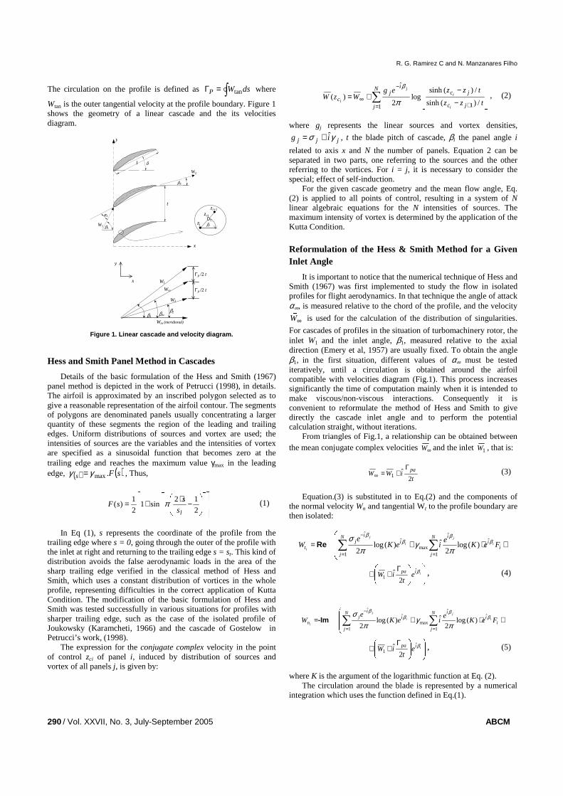
The circulation on the profile is defined as ∫=Γ dsWP tan where

Wtan is the outer tangential velocity at the profile boundary. Figure 1 shows the geometry of a linear cascade and the its velocities diagram.

l β

t

α1

β2

β1

y

x

βjzj

zj+1

zcj

W2

W1

β1β∞

β2

W∞

W2

W1

Γp /2 t

Γp /2 t

Wm (meridional)

x

y

Figure 1. Linear cascade and velocity diagram.

Hess and Smith Panel Method in Cascades

Details of the basic formulation of the Hess and Smith (1967) panel method is depicted in the work of Petrucci (1998), in details. The airfoil is approximated by an inscribed polygon selected as to give a reasonable representation of the airfoil contour. The segments of polygons are denominated panels usually concentrating a larger quantity of these segments the region of the leading and trailing edges. Uniform distributions of sources and vortex are used; the intensities of sources are the variables and the intensities of vortex are specified as a sinusoidal function that becomes zero at the trailing edge and reaches the maximum value γmax in the leading edge, ( ) ( )sFs .maxγγ = , Thus,

−⋅+=2

12sin1

2

1)(

ls

ssF π (1)

In Eq (1), s represents the coordinate of the profile from the

trailing edge where s = 0, going through the outer of the profile with the inlet at right and returning to the trailing edge s = st. This kind of distribution avoids the false aerodynamic loads in the area of the sharp trailing edge verified in the classical method of Hess and Smith, which uses a constant distribution of vortices in the whole profile, representing difficulties in the correct application of Kutta Condition. The modification of the basic formulation of Hess and Smith was tested successfully in various situations for profiles with sharper trailing edge, such as the case of the isolated profile of Joukowsky (Karamcheti, 1966) and the cascade of Gostelow in Petrucci’s work, (1998).

The expression for the conjugate complex velocity in the point of control zci of panel i, induced by distribution of sources and vortex of all panels j, is given by:

∑= +

−

∞ −

−+=

N

j jc

jci

jc tzz

tzzegWzW

i

i

j

i

1 1

ˆ

/)(sinh

/)(sinhlog

2)(

π

β, (2)

where gj represents the linear sources and vortex densities,

jjj ig γσ ˆ+= , t the blade pitch of cascade, βi the panel angle i

related to axis x and N the number of panels. Equation 2 can be separated in two parts, one referring to the sources and the other referring to the vortices. For i = j, it is necessary to consider the special; effect of self-induction.

For the given cascade geometry and the mean flow angle, Eq. (2) is applied to all points of control, resulting in a system of N linear algebraic equations for the N intensities of sources. The maximum intensity of vortex is determined by the application of the Kutta Condition.

Reformulation of the Hess & Smith Method for a Given Inlet Angle

It is important to notice that the numerical technique of Hess and Smith (1967) was first implemented to study the flow in isolated profiles for flight aerodynamics. In that technique the angle of attack α∞, is measured relative to the chord of the profile, and the velocity

∞Wr

is used for the calculation of the distribution of singularities.

For cascades of profiles in the situation of turbomachinery rotor, the inlet W1 and the inlet angle, β1, measured relative to the axial direction (Emery et al, 1957) are usually fixed. To obtain the angle β1, in the first situation, different values of α∞ must be tested iteratively, until a circulation is obtained around the airfoil compatible with velocities diagram (Fig.1). This process increases significantly the time of computation mainly when it is intended to make viscous/non-viscous interactions. Consequently it is convenient to reformulate the method of Hess and Smith to give directly the cascade inlet angle and to perform the potential calculation straight, without iterations.

From triangles of Fig.1, a relationship can be obtained between the mean conjugate complex velocities ∞W and the inlet 1W , that is:

tiWW

pa

2ˆ

1

Γ+=∞ (3)

Equation.(3) is substituted in to Eq.(2) and the components of

the normal velocity Wn and tangential Wt to the profile boundary are then isolated:

+⋅+= ∑∑==

− N

ji

ii

iN

j

ij

t FeKe

ieKe

W i

j

i

j

i

1

ˆˆ

maxˆ

1

ˆ

)(log2

ˆ)(log2

ββ

ββ

πγ

πσ

Re

Γ++ iipa e

tiW βˆ

1 2ˆ , (4)

+⋅+= ∑∑

==

− N

ji

ii

iN

j

ij

n FeKe

ieKe

W i

j

i

j

i

1

ˆˆ

maxˆ

1

ˆ

)(log2

ˆ)(log2

ββ

ββ

πγ

πσ

-Im Γ++ iipa e

tiW βˆ

1 2ˆ , (5)

where K is the argument of the logarithmic function at Eq. (2).

The circulation around the blade is represented by a numerical integration which uses the function defined in Eq.(1).



∑=

∆=ΓN

jiipa sF

1maxγ , where iii zzs −=∆ +1 (6)

Equation (6) is substituted into Eqs. (4) and (5). Expressions for

the tangential and normal velocities in the control points in terms of the inlet velocity, with the adequate effect of the vortex distribution are then calculated:

+= ∑=

−i

j

i

iN

j

ij

t eKe

W ββ

πσ ˆ

1

ˆ

)(log2

Re ⋅+ +⋅⋅+ −

=∑ iii

jii

N

j

ii

ii

eeWePFeKe

i βββββ

πγ ˆˆ

11

ˆˆˆ

max1)()(log

2ˆ . (7)

+−= ∑=

−i

j

i

iN

j

ij

n eKe

W ββ

πσ ˆ

1

ˆ

)(log2

Im + +⋅⋅+ −

=∑ iii

jii

N

j

ii

ii

eeWePFeKe

i βββββ

πγ ˆˆ

11

ˆˆˆ

max1)()(log

2ˆ (8)

−−

=+ tzz

tzzK

jc

jczz

i

i

jic /)sinh(

/)sinh(

1),( , (9a)

t

sF

P

N

jii

⋅

∆

=∑

=

21 . (9b)

Equations (7) and (8) can be rewritten in matrix form:

{ } [ ]{ } { } { }1max tant WDBW ++= γσ , (10)

{ } [ ]{ } { } { }1

max norn WCAW ++= γσ . (11)

The brackets {} represent column vectors Nx1 and the square

brackets [ ] square matrices N × N . [A] and [B] are the matrices of the normal and tangential influence coefficient, respectively, that depend only on the geometry of the airfoil, the blade pitch, the stagger angle, and the number of panels; {D} and {C} represent the

vectors of the normal and tangential influence of vortex; { }tanW 1

and { }norW 1 are the vectors of the normal and tangential

components in the cascade inlet; { }nW is the vector of the normal

velocity imposed at the boundary of the profile. According to the method of Hess and Smith for the potential

flow around the bodies, the variables γmax (vortex) and σ (source) from Eqs. (10) and (11) are determined by the simultaneous application of the two conditions. The first is the boundary condition of the impenetrability that requires a null normal velocity over the body surface: 0=nW ; the second is the Kutta Condition that

requires a flow that doesn’t turn around the trailing edge. One way to impose this condition is to requires the tangential velocities on the control points over panels of the trailing edge to be the same, but in the opposite direction, that is, Wtn = -Wt1. The following chapter will treat the breakaway and the modifications of normal velocities of transpiration in the boundary condition as well as the Kutta’s Condition.

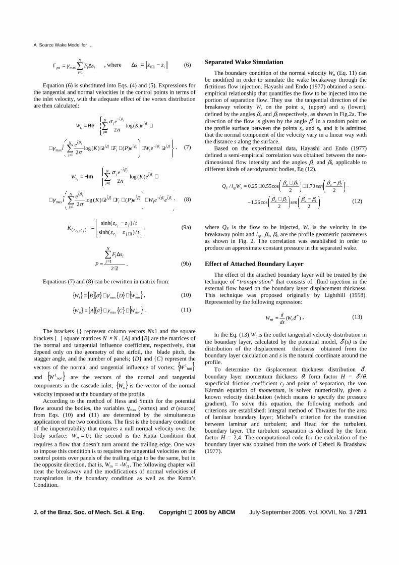
Separated Wake Simulation

The boundary condition of the normal velocity Wn (Eq. 11) can be modified in order to simulate the wake breakaway through the fictitious flow injection. Hayashi and Endo (1977) obtained a semi-empirical relationship that quantifies the flow to be injected into the portion of separation flow. They use the tangential direction of the breakaway velocity Ws on the point su (upper) and sl (lower), defined by the angles βu and βl respectively, as shown in Fig.2a. The direction of the flow is given by the angle β* in a random point on the profile surface between the points su and sl, and it is admitted that the normal component of the velocity vary in a linear way with the distance s along the surface.

Based on the experimental data, Hayashi and Endo (1977) defined a semi-empirical correlation was obtained between the non-dimensional flow intensity and the angles βu and βl, applicable to different kinds of aerodynamic bodies, Eq (12).

− −+ ++=2

70.12

cos55.025.0/ lulusspE senWlQ

ββββ − +−22

cos26.1 lulu senββββ (12)

where QE is the flow to be injected, Ws is the velocity in the breakaway point and lsp, βu, βl, are the profile geometric parameters as shown in Fig. 2. The correlation was established in order to produce an approximate constant pressure in the separated wake.

Effect of Attached Boundary Layer

The effect of the attached boundary layer will be treated by the technique of “transpiration” that consists of fluid injection in the external flow based on the boundary layer displacement thickness. This technique was proposed originally by Lighthill (1958). Represented by the following expression:

)( *δtnt Wds

dW = , (13)

In the Eq. (13) Wt is the outlet tangential velocity distribution in

the boundary layer, calculated by the potential model, δ*(s) is the distribution of the displacement thickness obtained from the boundary layer calculation and s is the natural coordinate around the profile.

To determine the displacement thickness distribution δ*, boundary layer momentum thickness θ, form factor H = δ*/θ, superficial friction coefficient cf and point of separation, the von Kármán equation of momentum, is solved numerically, given a known velocity distribution (which means to specify the pressure gradient). To solve this equation, the following methods and criterions are established: integral method of Thwaites for the area of laminar boundary layer; Michel’s criterion for the transition between laminar and turbulent; and Head for the turbulent, boundary layer. The turbulent separation is defined by the form factor H = 2,4. The computational code for the calculation of the boundary layer was obtained from the work of Cebeci & Bradshaw (1977).



βu

βl

β*θ

β1

su Wsp

Wt

W

W1

Wsp

Wnd

sl

lsp

Cp

x / l

1,0*Gx∆

Figure 2. (a) Definition of the normal velocity component, Wnd. (b) Agreement of the pressure distribution in the area of trailing edge, as Gostelow.

It is important to notice that the boundary layer code used in this

work doesn’t allow modeling the possible formation of displacement bubbles on the surface of the aerodynamic profile. This irregularity occurs when, at adverse pressure gradient, the laminar boundary layer is separated and subsequently, reattached in a turbulent condition. For example, it is possible to detect the circulation bubbles in the experimental curves of pressure coefficient in the NACA 65 profile cascades, operating with an intermediate Reynolds number around 105 (Emery et al, 1957). The clue is to identify the tendency of the formation of a constant pressure platform after the minimum pressure point on the profile suction side (that normally limits the end of the stable laminar area). The well successful modeling of the separated bubble, remains as an opened theme, requiring further development, beyond the scope of this work.

Wake Simulation for Small Angles of Attack

Gostelow’s correction was introduced like as correction method for the potential flow in a way to simulate the viscous effects. This correction aims to reduce the circulation and so to obtain more realistic values of the pressure and lift coefficients. The correction was proposed by Gostelow (1974) and consists of fairing–in the pressure distribution to avoid non-natural strong pressure gradients at the trailing edge region. The distance from the trailing edge where the adjustment is made is denoted as *

Gx∆ , as shown in Fig. (2b) in

the pressure coefficient curve, CP, as function of non-dimensional abscissa, x/l. Admitting the assumption that the value of

*Gx∆ represents the measure of viscous effect at the trailing edge

region, parameters were established for the aerodynamic load, capable to quantify those effects and consequentially to determine the value of *

Gx∆ . According to Lieblein (1959) correlation’s, the

diffusion rate is a measure of the aerodynamic load, which can be used to quantify the value *

Gx∆ . Lieblein defines the potential

diffusion rate Dpot as the relation between the maximum potential velocity value at suction side and the mean flow velocity at the cascade outlet. Analyzing the boundary layer, Lieblein obtained an empirical correlation from which it is possible to calculate the

variation of *Gx∆ with diffusion rate: )ln1/( 21

*potG Dkkx −=∆ where

89.02 =k and 020.01 =k are optimal regression factors based on

experimental data of diffusion *Gx∆ rate. Details of such analysis can

be found in Manzanares (1994) work. Such correlation will be applied for situations where the suction side flow doesn’t separate from the profile, remaining attached until the trailing edge. In these cases the modeling of a small wake next to trailing edge is necessary to avoid the uncontrolled rise of the boundary layer in this area. This work has, as an objective, directed to the effective design of turbomachinery and not specifically to the modeling of complex wakes and can be considered as a very simplified attached wake model. The idea is to use the own flow injection proposed by Hayashi and Endo (1977) to simulate the effect in this wake using a

small area established by the distance of Gostelow,*Gx∆ as the

injection area. The wake will be considered separate when the separation point is detected upstream the corresponding Gostelow

adjust abscissa *Gx∆ . Otherwise it will be considered a wake of

trailing edge.

Extended Hess and Smith Method for Aerodynamic Profiles With and Without Separation

The proposed extension my be used at any portion of the attached boundary layer considering the corresponding viscous effects quantified through the transpiration technique. In the separation area the extension will have value only for profile suction side breakaway situations. In this area the theoretical injection flow QT is given by separated normal velocities (Wnd) and by the length ∆S of the outline distance with separation, assuming that the velocity Wnd raises linearly from zero at the separation point:

2/i

N

pindT SWQ

s

i∆= ∑

=

, (14)

where: ps is the index that represents the separation point (random beginning), ∆S is the length along the profile surface in the breakaway area, and N the number of panels.

Connecting appropriately Eqs. (14) and (12) and incorporating the transpiration velocities, one has:

}{}{),(2

}{ ntsep

slun WS

l

WfW +=

ββ (15a)

{ } }{}{ ntsn WWKW += ,{ } { }Sl

fK

sep

lu ),(2 ββ= , (15bc)

where Ws is the separation velocity and {S} is the local coordinate vector of the separation area from the separation point. In Eq. (15b) the first term of the right represents the normal injection velocity vector that is a function of the separation velocity Ws and of the geometrical parameters: βu, βl, Isep and Si. The second term, the transpiration velocity of the attached boundary layer, is the vector of normal velocity around the aerodynamical body Wn. It is possible to substitute the outline assumption of Wn (Eq. 15b) in Eq. (11), resulting in the following matrix equations:

{ } { } [ ]{ } { } { }1max nornts WCAWWK ++=+ γσ , (16)

{ } [ ]{ } { } { }1max tant WDBW ++= γσ . (17)

Substituting the source intensity σ from Eq. (16) in Eq. (17):



{ } [ ] [ ] { } { }( ) { }( )+++−= − 111tanntnort WWWABW

[ ] [ ] { } { }( ) [ ][ ] { }KABWDCAB s11

max−− ++−+γ (18)

Making all the matrix operations on the Eq.(18), it results:

{ } { } { } { }VNORWVGAMAVINFW st ++= maxγ (19) Note that in Eq. (19), vortex intensity γmax and the velocity Ws

are unknown which may be calculated by a change in the Kutta’s condition, that is, the velocity at the separation point Ws will be the same as the velocity at the trailing edge in the lower side; Ws =Wps=-W1. From Eq. (19), it can be obtained the system of two equations with two variables Ws and γmax, where the subscript 1 refers to the first panel of the trailing edge on the lower side and ps to the panel where the separation point is fixed.

111 VNORWVGAMAVINFW smaxs +γ+=− ; (20a)

spsspmaxsps VNORWVGAMAVINFW +γ+= (20b)

Solving the system (20ab), the values γmax and Ws are obtained:

111

111max VGAMAVNORVNORVGAMAVGAMAVGAMA

VINFVNORVNORVINFVINFVINF

sss

sss

ppp

ppp

+−−−

−++=γ (21)

s

ss

p

pps VNOR

VGAMAVINFW

−+

=1

maxγ. (22)

The value of the pressure coefficient, Cp, is calculated taking in

to count the component of the normal and tangential velocities:

2

1

2

1

tan1

1 −−=W

W

W

WC n

p. (23)

Algorithm for Calculation

The methodology for calculating the flow with separation in aerodynamic bodies, including the viscous effects, is based on two computational codes 1) The potential code for calculating the flow in cascades, based on the numerical technique of Hess & Smith with modifications to simulate the effect of the separated wake; 2) The boundary layer code to determine the separation point and transpiration velocities. The computational codes will be quickly described as follows:

For the code 1, is supplied initially: cascade solidity λ =l /t, stagger angle β, inlet angle β1, Reynolds number Re, number of panels N, and reference airfoil coordinates. An initial position for the separation point is also introduced, where a fictitious fluid injection is imposed. Initially the separation point must be fixed close to the trailing edge; the program, re-positions iteratively this point until reaches convergence with the separation point obtained through boundary layer calculation.

The modified potential flow calculation supplies new velocity distributions where the boundary layer code will be utilized to indicate the new separation point position at the airfoil suction side. The boundary layer code is utilized iteratively until convergence is achieved for the separation point fixed at the potential calculation. When 160 to 200 panels are used is verified a optimum convergence above the control point. However, for less panels it is necessary to consider as stop criterion the tolerance in the distance between the fixed point in the potential calculation and the one determinated by

the boundary layer code. For 80 panels, the maximum difference between the point fixed was two to three control points. After convergence was attained, the separation point distance, measured from the trailing edge, was less than the fairing-in Gostelow (1974). If the separation was not detected then the Gostelow fairing-in was used to simulate a small separated wake. At this level the code offers preliminary results for the potential pressure distributions model with influence of the separated wake.

After the region for injection was defined, a second iterative process is activated. Then the normal velocities of transpiration Wnt

were introduced in the region where the flow was attached. The normal velocity components are then obtained from the Lighthill equation, Eq (13). The transpiration velocity values are sub-relaxed in each iteration with selected relaxation factors FR:

Wnt(actual) ⇐ FR .Wnt(actual) +(1- FR)Wnt(anterior). (24)

The distributions of the transpiration velocity along the blade

and flow injection are calculated iteratively until satisfactory overall convergence is obtained. A means to check the convergence is the drag coefficient variation ( 610−≤− atualdantd CC ).

The flow deflection angle in the cascade is calculated using the effective circulation and blade spacing of the cascade (Fig. 1). The effective circulation is calculated by integral of tangential velocities around airfoil. In the region of separation the tangential velocity is obtained from separation velocity (constant) and normal velocity of flow injection, that is:

∫ ∑ ∆≅=Γ=

i

N

iittef sWdsW

1

(25a)

22nst WWW −= (25b)

The lift coefficient is calculated by integration of the pressure

and skin friction coefficients. The skin friction coefficient in the region of separation is considered null and the pressure coefficient is considered constant between the separation point and trailing edge. In the following examples this hypothesis appears explicitly in the diagrams of Cp versus x/l.

The computational program was developed in Fortran 95 using the IMSL® library as tools for the solution of the system linear equation, splines and functions of interpolation and extrapolation.

The time required for execution of the program was approximately 6 minutes in PC, Pentium II, 300 MHz processor, with an average of 160 - 200 panels. Increase of the number of panels among 500-700, the processing time can reach up to 20 minutes, with little improvement in the results.

Drag Coefficient

Based on the works of Speidel (1954) and Schlichting (1959), the loss coefficient 1ω is considered as direct function of drag coefficient, that is:

∞=

βλ

ωcos

1*

1dC

, (26)

∞= βββθ cos

cos

cos2

23

12

*1 bfdC , (27)



where bfθ is the boundary layer momentum thickness at the trailing

edge for the suction and pressure sides or the place where the boundary layer separation occurs, )()( pressurebfsuctionbfbf θ+θ=θ .

Either of the equations (26) or (27) may be used for determination of the dissipative effect in the cascade, that is,

1dC or ω . It is

important to notice that, ω decreases with cascade solidity λ and, in the case of isolated airfoil (λ= 0), drag exists but losses are absent.

Speidel (1954), from theory and experimental data, obtained one empirical correlation for determination of the additional boundary layer momentum thickness in the separation region, for suction side, θsep.

−= 9,02

1

2W

Wy s

tAsepθ , (28)

where: Ws is the separation velocity, calculated from Eq. (22), W2 is the cascades outlet velocity and ytA is half the profile thickness at the point of separation (y(suction)A + y(pressure)A =ytA), (Sanger 1973).

The value of boundary layer momentum thickness in the separation region θsep can be added to Eq. (27), resulting the total drag coefficient:

( ) ∞+= βββθθ cos

cos

cos2

23

12

1 sepbfdC , (29)

For the drag calculation, the integration of drag and pressure

coefficients, were not used, because lead to mistakes in the process of numerical integration. Such process depends strongly on the number of panel and kinematic parameters. In the case of cascades, the situation is much more serious, because drag force is defined by the mean velocity direction, which depends from the calculation. Therefore small mistakes in the determination of the direction of the velocity can introduce large errors in drag component, without substantially affecting the lift component that is dominant.

Pressure Drag Determination by Fluid Injection

It is possible to substitute the Speidel (29) formula with one more appropriate, based on the flow injection technique. A Kutta-Joukowski theorem extension has been proposed by Manzanares (2001) for bidimensional flow around any aerodynamic body when there is one region of fictitious flows. The classic solution for skin friction is not considered and only pressure drag will be considered in the separation region.

Manzanares (2001) proposed the following formulation to calculate pressure drag in the separated flow region:

lW

WWQC sE

injd 21

)()(2

1

∞−= , (30)

where, QE represents the flow injection, calculated from Hayashi correlation, Ws the separation velocity calculated from the Eq. (22), W∞ the vector-mean velocity (Fig. 2), W1 the velocity of blade row , and l the blade chord.

Equation (30) requires that Ws ≥ W∞. This constraint won’t be satisfied for small angles attack when a small wake separation is used to guarantee the convergence. Therefore, situations where Ws < W∞ will be considered without physical meaning, resulting in

0)(1=injdC .

To calculate the cascade drag, it is possible to add Eq. (30) to Speidel’s Eq. (27) without considering the wake shear stress, resulting:

)(*

111 injddd CCC += (31)

A detailed description can be found in Ramirez (2001).

Pressures Distribution and Cascade Deflection Examples of Application

For the validation present methodology, the calculation results were compared with experimental data of Emery et al (1957) for airfoils in cascades: NACA-(18)10, NACA-(12)10, NACA-(08)10, and NACA-(04)10. In this work, for each airfoil, three different stagger angles β and angles of attack α1, are shown.

Figures (3) to (7) show the, results of the distributions of pressures for the indicate α, inlet flow angle β1, (β 1=β + α1) and cascade solidity λ parameters. The potential flow injection and transpiration models are presented. Compared with experimental data. For all cases 200, panels and Reynolds number of 2,54 ×105 were used. Agreement with as Emery et al (1957) data is achieved.

Usually 20 to 50 iterations, with sub-relaxation factor of 0,1 was required to accomplish the inviscid-viscous interaction, with a time of processing between 4 and 7 minutes in a Personal Computer, Pentium II de 300 MHz.

The cases of very low angles attack were not considered in this work because the results of the distributions of pressure of the lower side of the airfoil differ strongly of experimental dates, due to separation of boundary layer in this side, as well as of the cases where it was detected the existence of bubbles in the pressure side of the airfoil.

The results show that velocities of transpiration influence significantly the pressure distribution, resulting in decrease of angle deflection until up to 1º with relation to the model of pure the flow injection. In addition, the model can foresee satisfactorily the base pressure and the maximum angles, of great importance for the turbomachinery cascade design. A Small angles of attack, the pressure distribution was adjusted according to the flow injection calculated by Gostelow criterion, to simulate the formation of the small wake through the injection of fluid.

It must be emphasized that Emery et al (1957) data have an experimental error of ± 0,5º for the cascade angle of at design point deflection. This value may be higher at the “stall” region.

The first case analyzed is the cascade NACA64-(18)10. Figure.3, shows the pressure distribution for small angle attack. Figure. 3a uses adjustment criterion of Gostelow to injection flow.

Figure. 3d shows good agreement for angle attack α1 ≈ 20o, where are detected the maximum values of deflection. In this case the flow injection should be increased in a controlled way. Nevertheless, referencing to the methodology indicated in this work, empiric calibrations of the injection deserve other attention kind that will be explained as an open problem.

As the previous case, the NACA65-(12)10 cascade results calculation are shown. Pressure distributions, Fig.4a, are calculated based at the fairing Gostelow criterion, and the other graphics the separation point was obtained from the boundary layer code.

It is important to emphasize, at Fig. 4c, that the model produces good results of base pressure, as well as the maximum deflection of cascade (Fig.4d).



0 0.2

0.4 0 .6

0.8 1

0.0

0.4

0.8

1.2

1.6

2.0

2.4

1-C

p α1=8,7o, β=36,3o

x/l (a)

0 0.2 0.4 0.6 0.8 1 0.0

0.4

0.8

1.2

1.6

2.0

2.4

1-C

p

x/l

α1=14,6o, β=30,4o

(b)

0 0.2 0.4 0.6 0.8 1

0.0

0.4

0.8

1.2

1.6

2.0

2.4

2.8

3.2

3.6

4.0

1- C

p

α1=21,7o β=23,3o

x/l (c)

8 10 12 14 16 18 20 22 α1 (inlet angle attack)

14

16

18

20

22

24

26

28

30

Potential Pres. methodology Experiment

∆β

β1=45o, λ=0,5 Re=3,54×105

(d)

Figure 3. (a,b,c) Pressure distribution: ---- Potential, Present Methodology, � Experiment (d) Cascade deflection angle; NACA65-(18)10 airfoil , ββββ1=45o, λλλλ =0,5 Re=3,54××××105.

0 0.2 0.4 0.6 0.8 1

0.0

0.4

0.8

1.2

1.6

2.0

2.4

S = 1 - C p 1

1- C

p

α1=5,1o β=39,9o

x/l (a)

0 0.2 0.4 0.6 0.8 1 0.0

0.4

0.8

1.2

1.6

2.0

2.4

1- C

p

α1=16,1o β=28,9o

x/l (b)

0 0.2 0.4 0.6 0.8 1 0.0 0.4 0.8 1.2 1.6 2.0 2.4 2.8 3.2

S = 1 - C p 1

1- C

p

x/l

α1=25,1o β=19,9o

(c)

4 6 8 10 12 14 16 18 20 22 24 26

10

14

18

22

26

30

34

38 ∆β Potential

Pres. methodology Experiment

α1(inlet angle attack)

β1=45o, λ=1,0 Re=3,54×105

(d)

Figure 4. (a,b,c) Pressure distribution: ---- Potential, Present Methodology, � Experiment (d) Cascade deflection angle; NACA65-(12)10 airfoil, ββββ1=45o,λλλλ =1,0 Re=3,54××××105.



0 0.2 0.4 0.6 0.8 1 0.0

0.4

0.8

1.2

1.6

2.0

2.4

1- C

p

α1=9,7o β=35,3o

x/l (a)

0 0.2 0.4 0.6 0.8 1 0.0

0.4

0.8

1.2

1.6

2.0

2.4

1- C

p

. α1=13,7o β=31,3o

x/l (b)

0 0.2 0.4 0.6 0.8 1 0.0

0.4

0.8

1.2

1.6

2.0

2.4

2.8

3.2

S = 1 - C p 1

1- C

p

α1=22,7o β=22,3o

x/l (c)

6 8 10 12 14 16 18 20 22 24

12

14

16

18

20

22

24

26

28

30 ∆β Potential

Pres. methodology Eexperiment


β1=45o, λ=1,0 Re=3,54×105

(d)

Figure 5. (a,b,c) Pressure distribution: ---- Potential, Present Methodology, � Experiment (b) Cascade deflection angle; NACA65-(08)10 airfoil , ββββ1=45o, λλλλ =1,0 Re=3,54××××105.

0 0.2 0.4 0.6 0.8 1 0.0

0.4

0.8

1.2

1.6

2.0

2.4

2.8

S = 1 - C p 1

1- C

p

α1=4,0o β=56,0o

x/l (a)

0 0.2 0.4 0.6 0.8 1 0.0

0.4

0.8

1.2

1.6

2.0

2.4

2.8

S = 1 - C p 1

1- C

p

α1=6,0o β=54,0o

x/l (b)

0 0.2 0.4 0.6 0.8 1x/l

0.0

0.4

0.8

1.2

1.6

2.0

2.4

2.8

3.2

3.6

4.0

S = 1 - C p 1

1- C

p

α1=15,0o β=45,0o

(c)

0 2 4 6 8 10 12 14 16

0

2

4

6

8

10

12

14 ∆β Potential

Pres. methodology Experiment


β1=45o, λ=0,5 Re=3,54×105

(d)

Figure 6. (a,b,c) Pressure distribution: ---- Potential, Present Methodology, � Experiment (d) Cascade deflection angle; NACA65-(04)10 airfoil, ββββ1=45o, λλλλ =0.5 Re=3,54××××105.



Figures 5a and 5b, (NACA65-(08)10), point the influence of the flow injection for low angles attack, causing reduction of regions of constant pressure at suction side, stimulating the decrease of effective circulation, resulting in more real values of cascade deflection, (Fig 5d). Notice that, airfoil NACA65-(08)10, was the one that the methodology represented better the experimental results, of angle deflection as well as of angles attack from 8o to 23o. Verifying therefore that, Hayashi et al (1977) correlation are appropriate.

Finally it is analyzed a few cambered profiles, NACA65-(04)10. For flows with angles small attack (Fig. 6a) the potential pressure distributions approach experimental data. However, in the regions of large separation, the model represents better the experimental results, (Fig 6c). Note that present methodology satisfactorily describes the linear variation of the cascade deflection, (Fig.6d).

Lift and Drag Coefficients

Methodology validation also included, lift coefficient calculated by pressure and friction integration, and different calculations of drag coefficient, by Speidel (1954) correlation and by the flow injection formula.

The calculated points of aerodynamic coefficient (drag and lift) correspond to pressure distributions showed on Figures 3 to 6. The results are compared with Emery et al (1957) experimental data. The Cl /Cd maximum ratio is also shown because it defines the optimum condition of cascade performance, representing the maximum aerodynamic load with controlled drag forces.

The experimental drag measurement must be analyzed before they can be used for comparisons, because numerical values are relatively small and possibly large uncertainties due to measurement technique. The same must be applied to Cl /Cd ratio. More important here is the comparison of Cl /Cd relation with attack angle variations, and the possibility to find the optimum cascades with certain confidence, from Cl /Cd maximum relation.

In Figs. 7a to 7d shown the following results: lift coefficient Cl,

drag coefficients )2(dC (according Speidel) and the drag coefficient,

obtained according to flow injection criteria )3(dC . In the upper

portion of the figures, are the different values of )2(/ dl CC e )3(/ dl CC

compared with experimental data (Emery et al 1957). For all cases the lift values calculated from the potential model

are shown, indicating the large differences of experimental data, as already expected.

Fig. 7a shows the aerodynamic coefficients for NACA65-(18)10 profile. Notice that the model can satisfactorily foresee stall for an angle attack around 20o, corresponding to the maximum lift values. The drag curves, indicate notice that the calculated values (Speidel,

1954), )2(dC , and by flow injection, )3(

dC , have similar behavior.

However, the drag according to (Speidel), approaches experimental data on the region of lower of angles attack. The corresponding

maximum values of )2(/ dl CC and )3(/ dl CC occur practically at the

same of angle attack. However, the values )2(/ dl CC are closer to the

experimental data. Fig. 7b shows the aerodynamic coefficients for NACA65-(12)10

profile. The model reproduces lift values with agreement with experimental data. For small angles attack, where the flow injection is given by the Gostelow (1974) fairing, the model works adequately. For higher angles, flow injection criterion is used and results are equally satisfactory, especially at the maximum lift values. However, these results could be improved by flow injection calibration procedure in order to satisfy more adequately the lift values for the whole range of angle of attack. Calculated drag

values according Speidel and flow injection model show similar behavior on the regions of lower angles attack.

Figures 7c and 7d show aerodynamic coefficients (lift and drag) of NACA65-(08)10 and NACA65-(04)10 profiles. Notice the good agreement of lift coefficient in the whole range of angles of attack. Drag values calculated by the Speidel correlation and by flow injection formula approach experimental data on the lower range angles attack. For higher angles, the flow injection formula tends to underestimate the drag. When, the maximum values of

)3(/ dl CC relation tend to occur at angles nearer )2(/ dl CC stall values.

6 8 10 12 14 16 18 20 22

0.8

1.0

1.2

1.4

1.6

1.8

2.0

2.2

0 0.02 0.04 0.06 0.08

Cd

20 40 60 80 100

Cl

/Cd

Cl

NACA65-(18)10, β1=45o, λ=0,5


4 6 8 10 12 14 16 18 20 22 24 26

0.2

0.3

0.4

0.5

0.6

0.7

0.8

0.9

1.0

1.1

1.2

1.3

0

0.01

0.02

0.03

0.04

0.05

0.06

20

40

60

80

100

Cl Cd

Cl

/Cd

NACA65-(12)10, β1=45o, λ=1,0


Figure 7.- Lift and drag coefficients: --- Cl (1) potential, −−−−�−−−− Cl (1) experimental, −−−−�−−−− Pres. methodology , --�-- Cd experimental, −−−−�−−−−

(2)dC (Speidel), −−−−�−−−− (3)

dC (Inj. Flow), � Cl / Cd experimental, −−−−-−−−− (2)d/ClC ,

−−−−�−−−− )d/ClC (3 .



6 8 10 12 14 16 18 20 22 24 0.2

0.3

0.4

0.5

0.6

0.7

0.8

0.9

1.0

1.1

1.2

1.3

0

0.02

0.04

0.06

0.08

20

40

60

80

Cl

Cl /C

d

Cd

NACA65-(08)10, β1=45o, λ=1,0

α1 (inlet angle attack)

2 4 6 8 10 12 14 16 -0.2

0.0

0.2

0.4

0.6

0.8

1.0

1.2

1.4

1.6

0

0.01

0.02

0.03

0.04

0.05

20

30

40

50

60

70

Cl

Cl

/Cd

Cd

NACA65-(18)10, β1=45o, λ=0,5


Figure 7. (Continued).

Fig. 7c, shows that, the maximum )2(/ dl CC values are closer

to )3(/ dl CC experimental values, whereas, in Fig. 7d, the and

deflection angles. The drag calculation is more difficult to de situation is reversed. It is concluded that the methodology presented in this work can predict satisfactorily the lift coefficients calculated. The comparison between the procedures presented here, for the drag calculation is not conclusive yet and suggests the necessity of further systematic studies

Conclusions

The Hess & Smith (1967) method modified to simulate the flow in cascades, using the flow injection technique and transpiration velocities, produced satisfactory results for pressure distributions, cascade deflection angles, and lift coefficient. The results showed the strong influence of flow injection essentially near the stall region. The inviscid-viscous interaction was proved to be efficient with the use of relaxation techniques on normal transpiration velocities. On the other hand, the methodology is more efficient with the use of Hess & Smith panel technique where the cascade inlet velocity is used directly, to determine singularities distributions.

The methodology for the calculation of cascade flow presented in this work is based on contour integration formulation, having as vantage the small computation cost in relation to the full Navier Stokes equations solution. This method can be physically more realistic, but have higher computation cost. The present model is a low cost tool for initial design of the turbomachine cascades.

References.

Anderson, W.,K.,Thomas, J.L., Van Leer, B., 1986, “A Comparison of Finite Volume Flux Vector Splittings for the Euler Equations, “ AIAA Journal, Vol. 24, No 9, pp. 1453-1460.

Barnett, M., Hobbs, D.E., Edwards, D.E., 1991, “Inviscid – Viscous Interaction Analysis of Compressor Cascade Performance”, Transactions of the ASME, vol 113. pp. 538-552.

Bizarro, A.F., 1998, “Iteração Viscosa – não – Viscosa na Análise do Escoamento em Grades Lineares de Máquinas de Fluxo Axiais” , Tese de Mestrado, Instituto Tecnológico de Aeronáutica, Girardi R. (Orientador) São Jose dos Campos-Brasil.

Cebeci, T., Bradshaw, P., 1977, “Momentum Transfer in Boundary Layers”, McGraw-Hill/Hemisphere, Washington, D.C.

Emery, J.C., Herrig, L.J., Erwin, J. R., Felix, R., 1957, “Systematic Two- Dimensional Cascade Tests of Naca 65- Series Compressor Blades at Low Speeds”, NACA TN 1368.

Geller, W., 1972, “Incompressible Flow Through Cascades With Separation”, AGARD 167, Paper I-9, pp. 171-186.

Gostelow, J,P., 1974, “Cascade Aerodynamics ”, Pergamon Press Ltd., New York

Hansen, E.C., Serovy, G.K., Sockol, P.M., 1980, “Axial Flow Compressor Turning angle and loss by Inviscid/Viscous Interaction Blade to Blade Computation”, Transactions of the ASME, Vol. 102.

Hayashi, M., Endo, E., 1977, “Performance Calculation for Multi-Element Airfoil Sections with Separation”, Trans. Japan Soc. Aero. Space Sci.,Vol. 20, Nro 49.

He, L., Denton, J. D., 1994, “Tree Dimensional Time – Marching Inviscid and Viscous Solutions for Unsteady Flow Around Vibrating Blades”, Journal of Turbomachinery, Vol. 116, 469-476.

Hess, J.L., Smith, A.M.O., 1967, “Calculation of potential Flow About Arbitrary Bodies”, Progress in Aeronautical Sciences, Pergamon Press, Vol. 8, pp. 1-138.

Jones, K.M., Biedron , R. T., Whitlock, M., 1995, “ Application of a Navier Stokes Solver to the Analysis of Multielement Airfoils and Wings Using Multizonal Grid Techniques” , AIAA, Paper 95-1855.

Karamcheti., K., 1966, “Principles of Ideal-Fluid Aerodynamics”, John Wiley & Sonc. Inc., New York.

Lieblein S., 1959, “Loss and Stall Analysis of Compressor Cascades”, Journal of Basic Engineering, pp. 387- 400.

Lighthill, M.J., 1958, “On displacement Thickness”, J.F1 Mech., 4, pp. 383.

Manzanares Filho, N., 1994, “Análise do Escoamento em Maquinas de Fluxo Axiais”, Tese de Doutorado, Instituto Tecnológico de Aeronáutica ITA, São José dos Campos - Brasil.

Mathias, D.L., Roth, K., Ross, J.C., Rogers, S. E., Cummings, R.M., 1995, “Navier –Stokes Analysis of the Flow About a Flap-Edge” AIAA Paper 95-0185,.

Petrucci, R.D., 1998, “Problema Inverso do Escoamento em Torno de Perfís Aerodinâmicos Isolados e em Grade de Turbomaquinas”, Tese de Mestrado, UNIFEI, Itajubá-Mg, Brasil.

Ramirez R.G.C., 2001, “Análise do Escoamento em Grades de Turbomáquinas Axiais Incluindo o Efeito de Separação da Camada Limite”



(In Portuguese), Tese Doutorado, Escola Federal de Engenharia de Itajubá, M.G

Ramirez, R.G., Manzanres, N.F., Petrucci, D.R., 2000, “Extensão do Método de Hess & Smith para Cálculo do Escoamento em Grades com Separação”, Anais-CD, VIII Congresso Brasileiro de Ciências Térmicas, ENCIT 2000, Porto Alegre - Brasil.

Ramirez, R.G., Petrucci, D.R., Manzanares N.F., 1999, “Um Modelo de Escoamento Potencial para Cálculo da Distribuição de Pressões em Torno de Aerofólios com Separação Massiva”, Anais IV Congreso Iberoamericano de Ingenieria Mecanica, CIDIM 99, vol 3- Termofluidos, Santiago – Chile.

Roe, P.L., 1981, “Approximate Riemman Solvers, Parameter Vectors, and Difference Schemes.” , Journal of Computational Physics, Vol.43, No 3, pp. 357-372.

Roger E.S., Karlin R., Nash M. S. 2001, “Validation of Computed High-Lift Flow with Significant Wind-Tunnel Effects”, AIAA Journal, Vol.39, No 10, pp. 1884-1892.

Sanger N.L., 1973, “ Two-Dimensional Analytical and Experimental Performance Comparison for a Compressor Stator Section With D- Factor of 0.47” , NASA Technical Note, TN D-7425, pp. 1 –40.

Schlichting, H., 1959, “Application of Boundary – Layer Theory in Turbomachinery” Journal of Basic Engineering, pp. 543-551.

Spalart.,P.R., Allmaras, S.R., 1992, “A One-Equation Turbulence Model for Aerodynamics Flows”, AIAA Paper 92-0439.

Speidel, L., 1954, “Berechnung der Strömungsverluste von Ungestaffelten Ebenen Schaufelgittern. Dissertation, T. H. Braunschweig, 1953; Ing. Archiv, Vol. 22.

Documents

R. G. Ramirez C and N. Manzanares Filho A Source …R. G. Ramirez C and N. Manzanares Filho 290 / Vol. XXVII, No. 3, July-September 2005 ABCM The circulation on the profile is defined