F e v e r e i r o 2 0 1 5

416

EGARCH-RR: Realized Ranges

Explaining

EGARCH Volatilities

Victor Bello Accioly Beatriz Vaz de Melo Mendes

1

Relatórios COPPEAD é uma publicação do Instituto COPPEAD de Administração da Universidade Federal do Rio de Janeiro (UFRJ) Editora Leticia Casotti Editoração Lucilia Silva Ficha Catalográfica Cláudia de Gois dos Santos

A171c Accioly, Victor Bello.

EGARCH-RR: realized ranges explaining EGARCH volatilities / Victor Bello Accioly, Beatriz Vaz de Melo Mendes. – Rio de Janeiro: UFRJ /COPPEAD, 2015.

25 p.; 27 cm. – (Relatórios COPPEAD; 416) ISBN 978-85-7508-106-8 ISSN 1518-3335 1. Mercado de ações - Brasil. I. Mendes, Beatriz Vaz de

Melo. II. Título. III. Série.

CDD: 332.63222

2

EGARCH-RR: Realized Ranges explaining EGARCH volatilities

Victor Bello Accioly

COPPEAD - Federal University at Rio de Janeiro, Brazil.

Beatriz Vaz de Melo Mendes

IM/COPPEAD - Federal University at Rio de Janeiro, Brazil.

Abstract

The purpose of this paper is to investigate whether the inclusion of a realized measure

of volatility as external regressor on the GARCH and EGARCH variance equation would

result in more accurate fits. The estimation of the model is performed by maximum

likelihood with fifteen daily volatility series incorporated in the variance equation one at

a time. The results show that the realized volatility measures add information to the

EGARCH process; particularly, the realized range estimators that seem to outperform

the realized volatility one. The scaling approach appears to be superior to the others that

include squared overnight returns. GARCH is the most-adopted volatility model, which

in itself justifies any improvement attempting. Besides, to the best of our knowledge, this

is the first work to include range estimators to the EGARCH variance equation.

Keywords: GARCH; EGARCH; Realized Volatility; Realized Range; Brazilian stock mar-

ket.

JEL subject classifications: C22, C58, C32.

1

Resumo

O proposito do artigo e investigar se a inclusao de medidas de volatilidade realizada como

regressor externo na equacao de variancia dos modelos GARCH e EGARCH resultaria em

melhores ajustes. A estimacao e realizada pelo metodo de maxima verossimilhanca com

quinze series de volatilidade incorporadas na equacao de variancia uma de cada vez. Os

resultados mostram que medidas de volatilidade realizada adicionam informacoes para o

processo EGARCH, principalmente os estimadores realized range que parecem ter melhor

desempenho do que os realized volatility. A abordagem de um fator parece ser superior a

que incluı o retorno overnight ao quadrado. O GARCH e o modelo de volatilidade mais

adotado, o que por si so ja justifica qualquer tentativa de melhoria. Alem disso, de acordo

com o nosso conhecimento, esse e o primeiro trabalho a incluir estimadores de intervalo

na equacao de variancia EGARCH.

Palavras-Chave: GARCH; EGARCH; Volatilidade Realizada; Realized Range; Bovespa

2

EGARCH-RR: Realized Ranges explaining EGARCH volatilities

1 Introduction

Volatility is a key piece in finance with significant role in investment, security val-

uation, risk management, and monetary policy making. Thus, most of the activity

in the research area of a financial institution is devoted to modeling and forecasting

of an asset volatility.

There are different volatility modeling approaches. In a comprehensive review

of the methodologies and empirical findings of 93 papers, Poon and Granger (2003)

classified the volatility forecasting methods in two broad categories, time series

models and option implied standard deviation. The first is composed of three well

known large classes of models: Historical volatility models, Generalized Autoregres-

sive Conditional Heteroscedasticity (GARCH) family, and Stochastic Volatility (SV)

models.

Since Engle’s (1982) seminal paper, which motivation was to provide a tool for

measuring the dynamics of inflation uncertainty, a long list of articles have empiri-

cally proved the usefulness of the GARCH family members, specially in-sample, in

areas of economics and social sciences (e.g., the works of Bollerslev (1986, 1987),

Engle et al. (1987), Nelson (1991), Glosten et al. (1993), and Hansen and Lunde

(2005a)). Nonetheless, its out-of-sample predictive ability was cast in doubt after

some unsatisfactory empirical results (e.g., Akgiray (1989), Kat and Heynen (1994),

Franses and Van Dijk (1995), Brailsford and Faff (1996) and Figlewski (1997)),

which were accredited to the disturbance caused by the inherent noise of the squared

innovation used as a proxy for the ex-post volatility in the comparison with the pre-

dictions in Andersen and Bollerslev (1998), whom, therefore, used a new measure

based on high-frequency returns, later called ”realized variance”, to show that daily

GARCH volatility models perform well and accounts for around half the variability.

Chou (2005) appointed the flexibility of GARCH’s volatility dynamics and its

easier estimation procedure as its strengths against SV models. Brandt and Jones

(2006) resumed the volatility forecasting difficulties in three main causes: sensitivity

to the volatility model specification; difficulty of correctly estimate the parameters;

and, volatility forecasts anchored at noisy proxies or at current level volatility esti-

mates.

3

The literature related to the GARCH models is such enormous, as well as the list

of acronyms resulted, that Bollerslev (2009) wrote a type of reference guide. Some

of the models, the ”range-based” ones, are related to the use of log price ranges, in-

stead of closing prices in the model estimation (e.g., Alizadeh et al. (2002), Bali and

Weinbaum (2005), Shu and Zhang (2006), Brandt and Diebold (2006), Brandt and

Jones (2006) and Chou (2005)). The log price ranges are better volatility proxies

than the log squared, or absolute, returns, for adding more information, particu-

larly in turbulent periods; besides, the log price ranges distribution can be very

well approximated by a Gaussian distribution, facilitating the maximum likelihood

estimation.

The work of Mandelbrot (1971) was the first attempt to use range in the finance

field; however, the work of Parkinson (1980) is the breakthrough for having estab-

lished a relation between the range and the constant diffusion, which resulted in a

volatility measure far more efficient than the classical closing prices only. Thereafter,

many studies have followed, as Garman and Klass (1980), Beckers (1983), Rogers

and Satchell (1991), Wiggins (1992), Kunitomo (1992), Yang and Zhang (2000),

Chou (2005), Martens and van Dijk (2007), Christensen and Podolskij (2007), and

Chou et al. (2010).

Several exogenous variables, as pointed out by Zivot (2008), have been shown

to improve the volatility forecasts when added to GARCH’s conditional variance

formula, such as trading volume, macroeconomic news announcements, overnight

returns, after hours volatility, implied volatility from option prices and realized

volatility.

Following Day and Lewis (1992) methodology, although adding the realized

volatility as exogenous variable in the variance equation instead of the implied

volatility, Zhang and Hu (2013) cast some doubt if the former could provide addi-

tional information to the volatility process. It is worthy note that previously, Hansen

et al. (2010) introduced the called Realized GARCH framework, which combines dif-

ferently a GARCH structure and a model for realized volatility, finding considerable

improvements when compared with the standard GARCH model. Applying this

model to quantile forecasts of the S&P 500 index, Watanabe (2012) reached that

the Realized GARCH model with the skewed Student’s t-distribution outperform

the other models in the research.

Some models incorporating daily, or weekly, ranges were found promising, such

4

as the GARCH Parkinson Range of Mapa (2003), the Conditional Autoregressive

Range of Chou (2005) and the Range-Based Autoregressive Volatility of Li and Hong

(2011). Moreover, Li and Hong (2011) and Watanabe (2012) suggested the use of

other realized measures of volatility such as the realized range. The Exponential

GARCH (EGARCH) was adopted in Brandt and Jones (2006) for having the ability

to capture the most important stylized characteristics of volatility series, a slight

superiority of its specification over plain GARCH, the simplicity with which handle

volatility asymmetry, and for its familiarity.

In this paper, we investigate whether the inclusion of realized range estimators

as exogenous variables in the variance equation of EGARCH, and GARCH, models,

according to Day and Lewis (1992) methodology, may result in better volatility

forecasts and more accurate one-step-ahead risk measures in the Brazilian market.

The contribution of this paper is threefold. First, we show that the realized range

and realized volatility estimators provide further information to EGARCH process.

Second, forecasting stock volatility is important, specially for derivative pricing.

Third, this study in an important emerging market provides valuable insights for

foreign investors interested in investing into such markets.

The remainder of this paper is organized as follows. The next section provides

the theoretical framework for the empirical analysis, including a brief discussion on

high-frequency data, the definitions of realized volatility and realized range, and also

a review of the GARCH class of models. Section 3 briefly describes the Brazilian

stock market and the data sets used in the study as well as discusses the empirical

results. Concluding remarks are contained in Section 4.

2 Literature Review

2.1 High-Frequency Data

The so called high-frequency data have recently become widely available despite the

processing of a massive data amount being very time consuming requiring better

hardwares and programming skills. Therefore, it is natural to question whether to

use it or not. Andersen et al. (1999) present evidences of significant improvements

in inter-daily volatility forecasts for exchange rate returns to justify its use. Another

reason may be the usefulness of intraday market risk evaluation to market partic-

ipants involved in frequent trading. Furthermore, So and Xu (2013) suggest that

5

professionals may include an intraday seasonal indexes in the GARCH models, and

incorporate realized variance and time-varying degrees of freedom to capture more

intraday information on the volatile market.

Andersen et al. (2012) advocated that the rich information contained in the

high-frequency data may be effectively exploited through the use of realized volatil-

ity measures. Several researches have been conducted to analyze alternative mea-

sures based on different assumptions and information sets, specially the properties of

volatility proxies based on intra-daily data sampled at different frequencies (e.g, An-

dersen and Bollerslev (1998), Engle (2000), Barndorff-Nielsen and Shephard (2002),

Meddahi (2002), Maheu and McCurdy (2011), Andersen et al. (2011)).

It is important to highlight that the use of high-frequency data to reveal prices

until transaction-to-transaction level increases the market microstructure effects,

which theoretical manifestation through the realized variance estimator is that the

estimator fails to converge to the ”true variance”, increasing without bound when

the sampling interval approaches the transaction-to-transaction level (Bandi and

Russell, 2008).

2.2 Realized Volatility

The term realized volatility was first used in Fung and Hsieh (1991) and Andersen

and Bollerslev (1998) to account for the sum of intraday squared returns at short

intervals used as a proxy for ”realised volatility”, or an indicative of future price

movements. The main reason for the new estimator was the interest in forecasting

the unobserved integrated volatility over time intervals. According with Diebold and

Strasser (2012), it has become popular due to being: model free, computationally

trivial and, in principle, highly accurate.

The Andersen et al. (2001b) framework assumes that the logarithmic asset price

increments evolve continuously through time according to a stochastic volatility

diffusion process; and, the sum of the intraday squared returns converges to the

integrated volatility through the quadratic variation theory. The estimator over a

time interval of 1-day is defined as

RVt(∆) =n∑j=1

r2t−1+j∆, (1)

6

where ∆ = 1/n is the sampling interval, n is the interval numbers in 1-day, and

rt−1+j∆ = pt−1+j∆ − pt−1+(j−1)∆ defines continuously compounded returns.

Under these assumptions including the absence of jumps and microstructure

noise, the ex-post realized volatility is an unbiased volatility estimator providing a

consistent measure of the integrated volatility when the sampling frequency theo-

retically goes to continuous basis.

In his seminal paper, Merton (1980) had already observed that, in the theoretical

limit of continuous observation, the variance could in principle be estimated without

error for any finite interval; however, the sampling frequency cannot be any higher

than transaction by transaction. This sampling issue was addressed for several stud-

ies (e.g., Zhou (1996), Andersen et al. (2003) and Meddahi (2002)) by attempting

to sample in intervals of five to thirty minutes. Hence, Bai et al. (2004) stated

that large amounts of high-frequency data are not necessarily translated into pre-

cise estimates due to microstructure noise, but instead there is an optimal sampling

interval.

By doing so, defining an optimal sampling interval, potentially valuable infor-

mations are lost. Some recent works (e.g., Zhang et al. (2005), Aıt-Sahalia et al.

(2005), Hansen and Lunde (2006), Bandi and Russell (2008) and Aıt-Sahalia et al.

(2011)) have used all information to estimate the volatility, what gave rise to a series

of robust realized variance estimators.

2.3 Realized Range Volatility

The works of Martens and van Dijk (2007) and Christensen and Podolskij (2007)

provided theoretical support for the integrated variance be estimated with the new

realized range estimator, which empirically seems to work better than the realized

variance with its efficiency being function of the interval sampling size.

The basis for the arise of this new estimator may, as pointed by Chou et al.

(2010), remote to the fact that models based only on closing prices ignores the

prices inside of the reference period. Hence, Parkinson (1980) came up with an

estimator exploring the price range derived under the assumption that the asset

price follows a simple diffusion model without a drift term in a daily periodicity

framework, which Martens and van Dijk (2007) later extended to any interval, in

particular to the intraday intervals employed by the realized variance.

7

The “Parkinson” realized range estimator is then defined as,

RRParkinsont (∆) =

1

4 ln 2

1/∆∑j=1

(uj − dj)2 (2)

uj = lnHj − lnOj dj = lnLj − lnOj (3)

where Hj, Lj and Oj are the highest, the lowest and the opening prices of the jth

interval on the tth trading day; and uj and dj are a kind of normalized high and

low prices.

In their work, Martens and van Dijk (2007) also extended the two best Garman

and Klass (1980) volatility estimators to realized range framework, which through

simulation experiments were appointed more efficiently than the previous one, de-

fined as:

RRGK1t (∆) =

1/∆∑j=1

[0.511(uj − dj)2 − 0.019[cj(uj + dj)− 2ujdj]− 0.383c2j ] (4)

RRGK2t (∆) =

1/∆∑j=1

[0.5(uj − dj)2 − (2 ln 2− 1)c2j ] (5)

cj = lnCj − lnOj (6)

where Cj is the close price of the jth interval on the tth trading day; and cj is a

kind of normalized close price; the other variables are defined in Eq.(3).

The (three) previous estimators were derived based on the zero drift price process

assumption. A version with a non-zero drift term is proposed in Rogers and Satchell

(1991),

RRRSt (∆) =

1/∆∑j=1

[uj(uj − cj) + dj(dj − cj)], (7)

where the variables are defined in equations (3) and (6).

8

2.4 GARCH Family Models

The autoregressive conditional heteroscedastic (ARCH) processes of Engle (1982)

was the first model to generalize the implausible assumption of constant one-period

forecast variance. The basic idea behind this model is that the asset return innova-

tions are serially uncorrelated and dependent, whose dependence could be described

by a function of its lagged quadratic values. A generalized version of this process,

allowing for longer memory and a more flexible lag structure, was proposed by

Bollerslev (1986).

2.4.1 The GARCH process

The Generalized Autoregressive Conditional Heteroskedasticity process, GARCH(p,q),

is given by

εt | Ψt−1 ∼ D(0, ht), (8)

ht = α0 +

q∑i=1

αiε2t−i +

p∑j=1

βjht−j, (9)

where εt denote a real-valued discrete-time stochastic process, Ψt the information

set (σ-field) of all information through time t, and D(0, ht) denotes a distribution

with mean zero and variance ht; besides, αi and βj are nonnegative parameters with

α0 and βj also different of zero.

The process defined by (8) and (9) is stationary if and only if(∑q

i=1 αi +∑p

j=1 βj < 1)

.

Hence, E(εt) = 0, cov(εt, εs) = 0 for t 6= s, and Var(εt) = α0

(1−

∑qi=1 αi −

∑pj=1 βj

)−1

.

The GARCH process innovation at time t may be defined as εt = rt − µt for a

log return series rt; or, another approach, referred in the literature as GARCH-in-

mean, considers that an asset return may depend on its own volatility (Engle and

Bollerslev, 1986):

rt = µ+ cht + εt, (10)

where the mean return µ and the new parameter c, called risk premium parameter,

are constants.

9

2.4.2 The Exponential GARCH

Based on the GARCH model limitation of responding equally to positive and neg-

ative innovations, i.e., assuming that only the magnitude of unanticipated excess

returns matters, Nelson (1991) proposed a model which responds asymmetrically

to positive and negative residuals. The new Exponential GARCH process with

weighted innovation g(εt) is given by,

ln (ht) = α0 +1 + β1B + · · ·+ βq−1B

q−1

1− α1B − · · · − αpBpg(εt−1), (11)

g(ε) ≡ θεt + γ [| εt | − E(| εt |)] , (12)

where α0, θ and γ are real constants; B is the lag operator such that Bg(εt) =

g(εt−1); 1 + β1B + · · · + βq−1Bq−1 and 1− α1B − · · · − αpBp are polynomials with

zeros outside the unit circle and have no common factors; εt and |εt| − E(|εt|) are

zero-mean i.i.d. random sequences. The E(|εt|) value depends on the εt distribution.

It is worthy note that the positiveness of the conditional variance is guaranteed by

this model specification differently of the GARCH model.

3 Data and Empirical Results

3.1 Data Description and Cleaning

Our dataset was obtained directly from BM&FBOVESPA, which trading scheme is

consisted of two trading sessions, regular session and after-market, both preceded

with pre-opening auction sessions. The continuous regular session begins at 10:00

and ends at 17:00 with its pre-opening session from 9:45 to 10:00. The after-market

is from 17:35 until 19:00 with its pre-opening session from 17:30 to 17:35. These

trading hours, in Braslia Time (BRT) time zone, are changed in view of the start of

daylight saving time by the addition of one hour.

The tick-by-tick transaction information (time, price and volume), from De-

cember 1st 2009 to March 23rd 2012, of the eight most liquid constituent stocks

of the Bovespa Index were used; i.e, PETR4 (Petrobras), VALE5 (Vale), TNLP4

(Telemar), USIM5 (Usiminas), BBDC4 (Banco Bradesco), CSNA3 (Companhia

Siderurgica Nacional), OXGP3 (OGX Petroleo) and ITUB4 (Itauunibanco).

10

3.2 Measure Construction

The earliest studies using realized volatility were based on exchange rate data, which

are available for the whole day (apart from weekends). When considering financial

instruments that are frequently traded only in part of the day, e.g., six to seven

hours daily, the realized measures of volatility have to be extended for accounting

the full day. Hansen and Lunde (2005b) considered three ways of doing it: scaling

the estimator and adding, or combining, the squared overnight returns.

Since trading frequency and volume are much lower during the after-market

session, and there is a 2% price variation boundary relative to the regular session

closing price, the realized measures are constructed based on ∆-frequency intervals

between the regular session hours only.

Therefore, there are three definitions of daily volatility in this paper, which are

functions of the volatility measure and sampling interval chosen:

σ12t = δRt (13)

σ22t = r12

t +Rt (14)

σ32t = ω1r1

2t + ω2Rt (15)

where Rt is one of the five realized measures of variance previously defined (i.e., at

equations (1), (2), (4), (5) and (7)), and r1t is the overnight return (i.e., the regular

session close-to-open return) on date t; δ is the volatility measure scale factor, ω1

and ω2 are optimal linear combination weights, or factors, that minimizes the Mean

Square Error (MSE),

δ =n∑t=1

(rt − r)2/

n∑t=1

Rt (16)

ω∗1 = (1− ϕ)µ0

µ1

ω∗2 = ϕµ0

µ2

(17)

where the relative factor ϕ =µ22η

21−µ1µ2η12

µ22η21+µ21η

22−2µ1µ2η12

, µ0 =∑n

t=1(rt− r)2/n, µ1 = E(r12t ),

µ2 = E(Rt), η21 =

∑nt=1(r12

t − µ1)2/n, η22 =

∑nt=1(Rt− µ2)2/n, and η12 =

∑nt=1(r12

t −µ1)(Rt − µ2)/n.

There are a total of 420 trading minutes in a normal trading day. Several studies

11

found the optimal choice of the sampling frequency ∆ for constructing the realized

variance estimator to be between one and thirty minutes (Andersen et al. (2001a,

2003), Hansen and Lunde (2006) and Bandi and Russell (2008)). We investigate

different choices of ∆ ∈ {1, 5, 10, 15, 20, 30, 60, 105, 210, 420} minutes and 1-

second for the construction of the realized range estimator, and some of them to the

realized variance.

3.3 Methodology

This paper applies the same methodology applied in Zhang and Hu (2013) and in

Day and Lewis (1992), which is the addition of external variables to a GARCH

(EGARCH) model variance equation in order to improve its explanatory power.

Specifically, each one out of fifteen realized measures of volatility – five types (Parkin-

son, GK1, GK2, RS and RV) times three definitions (σ12t , σ22

t and σ32t ) – is added

one at a time, in the logarithmic form, at the following two model specifications:

ht = α0 +

q∑i=1

αiε2t−i +

p∑j=1

βjht−j +m∑k=1

θk ln (σ2t−k) (18)

ln (ht) = α0 +

q∑i=1

αi|εt−1|+ γiεt−i√

ht−1

+

p∑j=1

βj ln (ht−j) +m∑k=1

θk ln (σ2t−k) (19)

where σ2t stands for one of the realized measures of volatility and m represents the

number of lagged external variance factors. Through the R environment (R Core

Team, 2013) and rugarch package (Ghalanos, 2013), used to perform the maximum

likelihood estimation across the fifteen daily volatility series for several ∆ sampling

intervals, m is chosen equal to 3 for PETR4 and ITUB4 cases and equal to 2 for

other cases.

The Akaike information criterion (AIC) is used, with the t-statistics for the

individual coefficients, to test the hypothesis of improvement by adding the realized

measure of volatility.

3.4 Empirical Results

After estimating the best GARCH and EGARCH models the realized measures of

volatility (σ2t ) are added and the model is re-estimated. The estimation results of

12

GARCH+σ2t models show that information is not added to the simple GARCH. For

parsimonious reasons, these results are not reported.

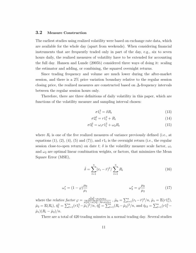
The Figure 1 graphs AIC versus ∆ sampling frequency in minutes for EGARCH

with realized range models. There are eight panels, each drawing one particular

asset, and three letters – P, G and R – coloured by blue, red and green colour. The

first letter represents Parkinson realized range type; the second, Garman and Klass

11; and the third, Rogers and Satchell. The blue dashed line marks the AIC for the

best EGARCH specification without external variance.

It is worth mentioning that nor for every ∆, the model estimations give reliable

results. The McCullough and Vinod (2003) procedures for nonlinear optimization

solution verification2 were followed. Even when a computer software package returns

a solution to an estimation problem, the solution may be inaccurate, or even does

not exist; then a verification procedure must be employed. The cases where accurate

solutions could not been found, with same model specification, were omitted from

the graph.

At a first glance to Figure 1, the red colour catches the eye. The red letters,

which represent the definition (14), are well separated from other colour letters,

usually concentrated at the panel top area, except for the TNLP4 case. This means

that σ22t tends to provide worse fits. The blue and green letters, which represent

the definitions (13) and (14) respectively, divide almost equally, and very close, the

numbers of winning combinations. The Parkinson realized range type dominates,

with five winning combinations, followed by Rogers and Satchell (two) and Garman

and Klass (one). The optimal sampling frequency seems to be somewhere between

one minute and thirty minutes.

Table 1 reports the estimation results of the winning combination for each asset.

The first column identify the case. The second and third columns present the AIC

for the EGARCH and EGARCH+RRt model. The next three columns show the

coefficients θ1, θ2 and θ3 with their standard error below. The RR and σ2t columns

identify the range and the volatility definition that compose the model. The last

three columns give the sampling interval (∆) and the squared overnight returns

(ωr12t ) and realized range (ωRt) weights respectively.

Analysing the results, since at least one of the θ coefficients for each asset is

significant at the 5% level, moreover the EGARCH+RRt model AIC is smaller than

the EGARCH one, there are plenty evidences that realized range provides additional

13

Figure 1: EGARCH+RR Fits: Sampling Frequency in minutes (∆) × Akaike information crite-rion (AIC).

Notes: Each of the eight panel represents one stock for several realized range model specifications, where:i) Parkinson, Garman and Klass 1, and Rogers and Satchell range types are labeled P, G and Rrespectively;ii) σ12t , σ22t , and σ32t , defined on (13), (14) and (15), are represented by blue, red and green coloursrespectively;iii) The blue dashed line ( ) represents the Akaike information criterion (AIC) for the bestEGARCH specification without external variance for each stock.

information content to EGARCH process.

Regarding to the realized variance, Figure 2 graphs AIC versus ∆ sampling

frequency in minutes for EGARCH with realized variance models. There are eight

panels, one per asset, with circles filled with blue, red or green colour. The blue

dashed line remain marking the AIC for the best EGARCH specification without

external variance.

At Figure 2, the red circle, which represent the definition (14), still well sep-

arated from other colours and concentrated at the panel top area, except for the

TNLP4 case. The σ22t seems to provide worse fits in most of the cases; however, for

the TNLP4 and ITUB4 cases, it constitutes the winning combination. Perhaps it

happens due to some particularity of the TNLP4 data and the scarcity of ITUB4

reliable fits. Once again the blue colour (σ12t ) excels. Although there are two cases

showing one second3 optimal sampling frequency, it might be related to same partic-

14

AssetAIC

θ1 θ2 θ3 RR σ2t ∆ ωr12

t ωRtEGARCH +RRt

PETR4 3.9096 3.87870.6798∗ -0.6229∗ 0.1678

P σ32t 20 0.2243 1.3772(0.1698) (0.2309) (0.1299)

VALE5 3.7710 3.75800.3811∗∗ -0.2322 –

P σ12t 20 0.0000 1.7618(0.1729) (0.1724)

TNLP4 4.0361 4.00310.4288∗ 0.3214∗ –

RS σ12t 420 0.0000 0.1401(0.1223) (0.1129)

USIM5 4.4677 4.43910.2014∗∗ 0.0001 –

P σ12t 105 0.0000 1.4009(0.0822) (0.0051)

BBDC4 3.7972 3.78070.4096∗ -0.2720 –

GK1 σ12t 30 0.0000 1.1427(0.1541) (0.1807)

CSNA3 4.2069 4.19330.4358∗ -0.4167∗ –

P σ32t 10 -0.0016 1.1853(0.1616) (0.1128)

OGXP3 4.6462 4.62830.6419∗ -0.5955∗ –

P σ32t 1 -0.0774 1.6177(0.1665) (0.1696)

ITUB4 3.8492 3.84030.5263∗ -0.6971∗ 0.1763

RS σ12t 1 0.0000 1.3078(0.1582) (0.2508) (0.1443)

Notes: i) Estimation results of EGARCH model with realized range measures in the variance equation.

ii) The report is based on estimation of the following model:

ln (ht) = α0 +∑qi=1 αi

|εt−1|+γiεt−i√ht−1

+∑pj=1 βj ln (ht−j) +

∑mk=1 θk ln (σ2

t−k)

iii) The columns AIC report EGARCH and EGARCH with realized range Akaike information criterion.

iv) The three coefficients θ1, θ2 and θ3 are reported with their standard error below. *, **,*** statistically significant at 1%, 5% and 10% levels respectively.

v) The RR column stands for the realized range estimator type, where P, GK1 and RS are,respectively, Parkinson, Garman and Klass 1, and Rogers and Satchell estimators.

vi) σ12t , σ22t , and σ32t refer to definitions (13), (14) and (15) respectively.

vii) ωr12t and ωRt stand for the weights in the linear combination.

viii) ∆ stands for the sampling frequency in minutes.

Table 1: The best EGARCH+Realized Range Fits

ularly from OGXP3 and ITUB4 cases, the optimal sampling frequency seems again

to be somewhere between one minute and thirty minutes.

The Figure 2 winning combination results are reported on Table 2, which follows

the same composition of the previous table, except for substituting RRt for RVt and

dropping the range type column.

The finding is confirmed with EGARCH+RVt model results. At least one of the

θ coefficients for each asset is significant at the 10% level4, as well as the AIC is

smaller than the EGARCH without external variable model.

15

Figure 2: EGARCH+RV Fits: Sampling Frequency in minutes (∆) × Akaike information crite-rion (AIC).

Notes: Each of the eight panel represents one stock for several realized volatility model specifications, where:

i) σ12t , σ22t , and σ32t , defined on (13), (14) and (15), are represented by blue, red and green coloursrespectively;ii) The blue dashed line ( ) represents the Akaike information criterion (AIC) for the best EGARCHspecification without external variance for each stock.

4 Conclusion

In this paper we empirically investigated whether or not the inclusion of realized

range and realized volatility estimators into the GARCH and EGARCH models vari-

ance equation provide additional information to the process. According to the liter-

ature, the range estimator tends to be more efficient than the squared return. Our

empirical findings are supported by the theory, the combinations between EGARCH

model and realized range estimator outperform the realized variance ones, except

for the OGXP3 and CSNA3 cases, which the squared overnight return factors are

negative.

Another concluding remarks linked to the extant literature that usually the op-

timal linear estimated weights of the realized measure of volatility are dispropor-

tionately larger when compared with the squared overnight return ones, is that σ22t ,

definition (14), constantly shows the worse results. However, as expected, when

16

AssetAIC

θ1 θ2 θ3 σ2t ∆ ωr12

t ωRtEGARCH +RVt

PETR4 3.9096 3.88400.7684∗ -0.8192∗ 0.2307

σ32t 1 0.0225 1.3764(0.2102) (0.3155) (0.1707)

VALE5 3.7710 3.76030.2521 -0.1056 –

σ12t 10 0.0000 1.9399(0.1543) (0.1514)

TNLP4 4.0361 4.00980.3761∗ -0.2561∗∗ –

σ22t 30 0.5000 0.5000(0.1103) (0.1227)

USIM5 4.4677 4.43930.1925∗∗∗ 0.0562 –

σ12t 10 0.0000 1.4762(0.1092) (0.1617)

BBDC4 3.7972 3.78720.2590∗∗∗ -0.1110 –

σ12t 5 0.0000 1.1985(0.1463) (0.1762)

CSNA3 4.2069 4.19300.3852∗ -0.3376∗∗ –

σ12t 10 0.0000 1.1882(0.1285) (0.1316)

OGXP3 4.6462 4.62510.6524∗ -0.6070∗ –

σ32t 0 -0.0826 0.3260(0.1635) (0.1669)

ITUB4 3.8492 3.84380.454∗ -0.6864∗ 0.236

σ22t 0 0.5000 0.5000(0.1527) (0.2474) (0.1521)

Notes: i) Estimation results of EGARCH model with realized volatility measures in the variance equation.

ii) The report is based on estimation of the following model:

ln (ht) = α0 +∑qi=1 αi

|εt−1|+γiεt−i√ht−1

+∑pj=1 βj ln (ht−j) +

∑mk=1 θk ln (σ2

t−k)

iii) The columns AIC report EGARCH and EGARCH with RV Akaike information criterion.

iv) The three coefficients θ1, θ2 and θ3 are reported with their standard errorbelow. *, **, *** statistically significant at 1%, 5% and 10% levels respectively.

v) σ12t , σ22t , and σ32t refer to definitions (13), (14) and (15) respectively.

vi) ωr12t and ωRt stand for the weights in the linear combination.

vii) ∆ stands for the sampling frequency in minutes, where 0 symbolize 1 second interval.

Table 2: The best EGARCH+Realized Volatility Fits

the squared overnight return contains some valuable information, σ32t tends to give

better fits than σ12t , definitions (15) and (13) respectively.

This methodology may be very useful at scenarios where high-frequency data are

not available, specially because realized volatility estimators are unfeasible at daily

intervals. At these scenarios the first choice to model an asset’s volatility tends to

be one across the GARCH family models, whose fits, as shown in the study, may be

improved with realized range estimators. the improvement happens even in absence

of high-frequency data, since the realized range estimators may be computed over

daily sampling intervals, and the information required – open, high, low and close

daily prices – are usually available.

These findings contrast with the doubt raised by Zhang and Hu (2013) on the

notion that realized volatility could have additional information than the GARCH

and EGARCH model. It might be explained by the former have included the square

17

root of σ22t definition into the EGARCH variance equation instead of the logarithmic

form. The difference between both emerging markets, Brazilian and Chinese, can

not be discarded as well.

It is important to highlight that these findings were based on an in-sample es-

timation. The out-of-sample performance needs to be investigated, in addition this

study should be expanded to other markets with larger series. A comparison against

option-implied volatility would also be interesting.

Notes

1The Garman and Klass 2 realized range type is not reported due to its observedsimilarity with Garman and Klass 1.

2i.e., vary the default options of the nonlinear solver by decreasing the tolerance,switching the convergence criterion, changing the algorithms and starting values.

3represented in the graph by its decimal minute approximation.

4The θ1 coefficient of VALE5 is significant as the 10.5% level.

References

Aıt-Sahalia, Y., Mykland, P. A., and Zhang, L. (2005). How often to sample a continuous-

time process in the presence of market microstructure noise. Review of Financial Stud-

ies, 18(2):351–416.

Aıt-Sahalia, Y., Mykland, P. A., and Zhang, L. (2011). Ultra high frequency volatility

estimation with dependent microstructure noise. Journal of Econometrics, 160(1):160–

175.

Akaike, H. (1973). Information theory and an extension of the maximum likelihood prin-

ciple. In Petrov, B. N. and Csaki, F., editors, Proceedings of the 2nd International

Symposium on information theory, pages 267–281, Budapest. Akademiai Kiado.

Akgiray, V. (1989). Conditional heteroscedasticity in time series of stock returns: Evidence

and forecasts. The Journal of Business, 62(1):55–80.

Alizadeh, S., Brandt, M. W., and Diebold, F. X. (2002). Range-based estimation of

stochastic volatility models. The Journal of Finance, 57(3):1047–1091.

18

Andersen, T. G. and Bollerslev, T. (1998). Answering the skeptics: Yes, standard volatility

models do provide accurate forecasts. International Economic Review, 39(4):885–905.

Andersen, T. G., Bollerslev, T., Christoffersen, P. F., and Diebold, F. X. (2012). Finan-

cial risk measurement for financial risk management. NBER Working Papers 18084,

National Bureau of Economic Research, Cambridge, MA, USA.

Andersen, T. G., Bollerslev, T., Diebold, F. X., and Ebens, H. (2001a). The distribution

of realized stock return volatility. Journal of Financial Economics, 61(1):43–76.

Andersen, T. G., Bollerslev, T., Diebold, F. X., and Labys, P. (2001b). The distribution

of realized exchange rate volatility. Journal of the American Statistical Association,

96(453):42–55.

Andersen, T. G., Bollerslev, T., Diebold, F. X., and Labys, P. (2003). Modeling and

forecasting realized volatility. Econometrica, 71(2):579–625.

Andersen, T. G., Bollerslev, T., and Lange, S. (1999). Forecasting financial market

volatility: Sample frequency vis-a-vis forecast horizon. Journal of Empirical Finance,

6(5):457–477.

Andersen, T. G., Bollerslev, T., and Meddahi, N. (2011). Realized volatility forecasting

and market microstructure noise. Journal of Econometrics, 160(1):220–234.

Bai, X., Russel, J., and Tiao, G. (2004). Effects of non-normality and dependence on the

precision of variance estimates using high-frequency financial data. Working papers,

University of Chicago.

Bali, T. G. and Weinbaum, D. (2005). A comparative study of alternative extreme-value

volatility estimators. Journal of Futures Markets, 25(9):873–892.

Bandi, F. M. and Russell, J. R. (2008). Microstructure noise, realized variance, and

optimal sampling. Review of Economic Studies, 75(2):339–369.

Barndorff-Nielsen, O. E. and Shephard, N. (2002). Estimating quadratic variation using

realized variance. Journal of Applied Econometrics, 17(5):457–477.

Beckers, S. (1983). Variances of security price returns based on high, low, and closing

prices. The Journal of Business, 56(1):97–112.

Bollerslev, T. (1986). Generalized autoregressive conditional heteroskedasticity. Journal

of Econometrics, 31(3):307–327.

19

Bollerslev, T. (1987). A conditionally heteroskedastic time series model for speculative

prices and rates of return. The Review of Economics and Statistics, 69(3):542–547.

Bollerslev, T. (2009). Glossary to ARCH (GARCH). In Bollerslev, T., Russell, J. R., and

Watson, M., editors, Volatility and Time Series Econometrics: Essays in Honour of

Robert F. Engle, pages 137–163. Oxford University Press, Oxford, UK.

Brailsford, T. J. and Faff, R. W. (1996). An evaluation of volatility forecasting techniques.

Journal of Banking & Finance, 20(3):419–438.

Brandt, M. W. and Diebold, F. X. (2006). A no-arbitrage approach to range-based esti-

mation of return covariances and correlations. The Journal of Business, 79(1):61–74.

Brandt, M. W. and Jones, C. S. (2006). Volatility Forecasting with Range-Based EGARCH

Models. Journal of Business & Economic Statistics, 24(4):470–486.

Chou, R., Chou, H., and Liu, N. (2010). Range volatility models and their applications in

finance. In Lee, C.-F., Lee, A., and Lee, J., editors, Handbook of Quantitative Finance

and Risk Management, pages 1273–1281. Springer US.

Chou, R. Y. (2005). Forecasting Financial Volatilities with Extreme Values: The Con-

ditional Autoregressive Range CARR Model. Journal of Money, Credit and Banking,

37(3):561–582.

Christensen, K. and Podolskij, M. (2007). Realized range-based estimation of integrated

variance. Journal of Econometrics, 141(2):323–349.

Day, T. E. and Lewis, C. M. (1992). Stock market volatility and the information content

of stock index options. Journal of Econometrics, 52(1–2):267–287.

Diebold, F. X. and Strasser, G. H. (2012). On the correlation structure of microstructure

noise: A financial economic approach. NBER Working Papers 16469, National Bureau

of Economic Research.

Engle, R. F. (1982). Autoregressive conditional heteroscedasticity with estimates of the

variance of united kingdom inflation. Econometrica, 50(4):987–1007.

Engle, R. F. (2000). The econometrics of ultra-high-frequency data. Econometrica,

68(1):1–22.

Engle, R. F. and Bollerslev, T. (1986). Modelling the persistence of conditional variances.

Econometric Reviews, 5(1):1–50.

20

Engle, R. F., Lilien, D. M., and Robins, R. P. (1987). Estimating time varying risk premia

in the term structure: The arch-m model. Econometrica, 55(2):391–407.

Figlewski, S. (1997). Forecasting volatility. Financial Markets, Institutions & Instruments,

6(1):1–88.

Franses, P. and Van Dijk, D. (1995). Forecasting stock market volatility using (non-linear)

GARCH models. Journal of Forecasting, 15:229–235.

Fung, W. K. and Hsieh, D. A. (1991). Empirical analysis of implied volatility: Stocks,

bonds and currencies. Working papers, Fuqua School of Business.

Garman, M. B. and Klass, M. J. (1980). On the estimation of security price volatilities

from historical data. The Journal of Business, 53(1):67–78.

Ghalanos, A. (2013). rugarch: Univariate GARCH models, R package version 1.2-7 edition.

Glosten, L. R., Jagannathan, R., and Runkle, D. E. (1993). On the relation between the

expected value and the volatility of the nominal excess returns on stocks. Journal of

Finance, 48(5):1779–1801.

Hansen, P. and Lunde, A. (2006). Realized variance and market microstructure noise.

Journal of Business & Economic Statistics, 24(2):127–161.

Hansen, P. R., Huang, Z. A., and Shek, H. H. (2010). Realized garch: A complete model of

returns and realized measures of volatility. CREATES Research Papers 2010-13, School

of Economics and Management, University of Aarhus.

Hansen, P. R. and Lunde, A. (2005a). A forecast comparison of volatility models: does

anything beat a GARCH(1,1)? Journal of Applied Econometrics, 20(7):873–889.

Hansen, P. R. and Lunde, A. (2005b). A realized variance for the whole day based on

intermittent high-frequency data. Journal of Financial Econometrics, 3(4):525–554.

Kat, H. M. and Heynen, R. C. (1994). Volatility Prediction: A Comparison of the Stochas-

tic Volatility, GARCH(1,1) and EGARCH (1,1) Models. Journal of Derivatives, 2(2).

Kunitomo, N. (1992). Improving the parkinson method of estimating security price volatil-

ities. The Journal of Business, 65(2):295–302.

Li, H. and Hong, Y. (2011). Financial volatility forecasting with range-based autoregressive

volatility model. Finance Research Letters, 8(2):69–76.

21

Maheu, J. M. and McCurdy, T. H. (2011). Do high-frequency measures of volatility

improve forecasts of return distributions? Journal of Econometrics, 160(1):69–76.

Mandelbrot, B. B. (1971). When can price be arbitraged efficiently? a limit to the validity

of the random walk and martingale models. The Review of Economics and Statistics,

53(3):225–236.

Mapa, D. S. (2003). A Range-Based GARCH Model for Forecasting Volatility. MPRA

Paper 21323, University Library of Munich, Germany.

Martens, M. and van Dijk, D. (2007). Measuring volatility with the realized range. Journal

of Econometrics, 138(1):181–207.

McCullough, B. and Vinod, H. (2003). Econometrics and sofware. The Journal of Eco-

nomic Perspectives, 17(1):223–224.

Meddahi, N. (2002). A theoretical comparison between integrated and realized volatility.

Journal of Applied Econometrics, 17(5):479–508.

Merton, R. C. (1980). On estimating the expected return on the market: An exploratory

investigation. Journal of Financial Economics, 8(4):323–361.

Nelson, D. B. (1991). Conditional heteroscedasticity in asset returns: A new approach.

Econometrica, 59(2):347–370.

Parkinson, M. (1980). The extreme value method for estimating the variance of the rate

of return. The Journal of Business, 53(1):pp. 61–65.

Poon, S.-H. and Granger, C. W. J. (2003). Forecasting volatility in financial markets: A

review. Journal of Economic Literature, 41(2):478–539.

R Core Team (2013). R: A Language and Environment for Statistical Computing. R

Foundation for Statistical Computing, Vienna, Austria.

Rogers, L. C. G. and Satchell, S. E. (1991). Estimating variance from high, low and closing

prices. The Annals of Applied Probability, 1(4):pp. 504–512.

Shu, J. and Zhang, J. E. (2006). Testing range estimators of historical volatility. Journal

of Futures Markets, 26(3):297–313.

So, M. and Xu, R. (2013). Forecasting intraday volatility and value-at-risk with high-

frequency data. Asia-Pacific Financial Markets, 20(1):83–111.

22

Watanabe, T. (2012). Quantile Forecasts of Financial Returns Using Realized GARCH

Models. Japanese Economic Review, 63(1):68–80.

Wiggins, J. B. (1992). Estimating the volatility of s&p 500 futures prices using the

extreme-value method. Journal of Futures Markets, 12(3):265–273.

Yang, D. and Zhang, Q. (2000). Drift-independent volatility estimation based on high,

low, open, and close prices. The Journal of Business, 73(3):477–91.

Zhang, J. and Hu, W. (2013). Does realized volatility provide additional information?

International Journal of Managerial Finance, 9(1):70–87.

Zhang, L., Mykland, P. A., and Aıt-Sahalia, Y. (2005). A tale of two time scales: Deter-

mining integrated volatility with noisy high-frequency data. Journal of the American

Statistical Association, 100(472):1394–1411.

Zhou, B. (1996). High-frequency data and volatility in foreign-exchange rates. Journal of

Business & Economic Statistics, 14(1):45–52.

Zivot, E. (2008). Practical issues in the analysis of univariate garch models. Working

Papers UWEC-2008-03-FC, University of Washington, Department of Economics.

23